System-Level Analysis of Joint Sensing and Communication based on 5G New Radio

Abstract

This work investigates a multibeam system for joint sensing and communication (JSC) based on multiple-input multiple-output (MIMO) 5G new radio (NR) waveforms. In particular, we consider a base station (BS) acting as a monostatic sensor that estimates the range, speed, and direction of arrival (DoA) of multiple targets via beam scanning using a fraction of the transmitted power. The target position is then obtained via range and DoA estimation. We derive the sensing performance in terms of probability of detection and root mean squared error (RMSE) of position and velocity estimation of a target under line-of-sight (LOS) conditions. Furthermore, we evaluate the system performance when multiple targets are present, using the optimal sub-pattern assignment (OSPA) metric. Finally, we provide an in-depth investigation of the dominant factors that affect performance, including the fraction of power reserved for sensing.

I Introduction

The widespread diffusion of increasingly broadband mobile radio networks and the conquest of mmWave by 5G communication systems has exacerbated the spectrum congestion. On the other hand, sensing capabilities via radio frequency (RF) signals are gaining increasing interest for several applications, such as autonomous driving, assisted living, security, and human-machine interface [2]. In the framework of this trend, we are witnessing an increasing demand for systems exhibiting both sensing and communications capabilities, i.e., systems where radar and communication functionalities share the hardware platform, as well as the frequency band [3, 4]. This approach is also known as JSC and consists in exploiting the waveforms transmitted by a communication network to perform sensing functions. In this scenario, orthogonal frequency division multiplexing (OFDM) based signals are considered good candidates both for active and passive radar purposes. For example, in [5] and [6] OFDM-based communication systems such as long term evolution (LTE) and 5G NR are suggested. In [7] the self-ambiguity function (SAF) and cross-ambiguity function (CAF) for the frequency division duplex (FDD) LTE downlink waveform are evaluated. Another possible solution, widely explored in literature, is represented by passive radars relying on signals of opportunity. In this case, the problem of the spectrum sharing is solved by removing the radar sources, i.e., by performing localization and tracking of targets without the need for radar signals emissions but only by exploiting illuminators of opportunity already present in the environment [8, 9]. However, the radar system does not have full knowledge about the transmitted signals and can only perform detection and estimation based on the power, angles, and Doppler information extracted from the received echo [10].

In [4] applications of JSC systems are discussed. According to [11], JSC can be studied focusing on both simple point-to-point communications such as vehicular networks [12, 13, 14, 15, 16, 17] (thus finding great applications in autonomous driving) and complex mobile/cellular networks [10, 18, 19, 20], which can potentially revolutionize the current communication-only mobile networks. JSC also has the potential of integrating radio sensing into large-scale mobile networks, generating the so-called perceptive mobile networks [21, 10, 22, 23, 24]. Moreover, literature on mmWave JSC demonstrates its feasibility and potentials in indoor and vehicle networks [25, 12, 26, 15, 27, 28, 29, 30]. In particular, in-depth signal processing aspects of mmWave-based JSC with an emphasis on waveform design are provided by [25]. At mmWave frequencies, MIMO systems enable very high capacity links and reduced latencies to the communication users through spatial multiplexing, while also providing augmented sensing capabilities due to accurate DoA estimation [31, 32].

Some research studies on JSC mainly focus on single beam approaches per phased array, having the sensing beam in the same direction of the communication beam [33]. To overcome this problem, recent studies have focused on using separate coexisting beams for communication and sensing due to the very different requirements of the two functionalities. For example, in [12, 34] a multibeam framework consisting of beamforming design and optimization are proposed to simultaneously allow a steady communication beam towards the user equipment (UE) and a sensing beam to scan the environment.

Most of the research efforts on JSC have so far been devoted to the design of signal processing techniques aimed at extracting features from the environment, such as the position and speed of a target (for example, a car or a human being) or at inferring the environment itself, such as the mapping or imaging of a room. However, to the authors’ knowledge, very few works have investigated the performance of a JSC system, especially from the sensing perspective, and provided results in terms of target parameters estimation accuracy with current technology. For this reason, this work aims to address the analysis of a multibeam system for JSC based on 5G NR to understand the key aspects and their role in governing performance. In particular, the main contributions are the following:

• We provide an analysis of the performance of a BS acting as a sensor in a monostatic configuration that estimates the range, speed, and DoA of multiple targets, through numerical simulations. In particular, we provide a detailed analysis of how the system performance is affected by the portion of the total radiated power used for sensing. Furthermore, we propose an algorithm to remove phantom targets that appear because of the sensing method, which relies on beam-scanning impaired by beam sidelobes.

• We analyze the root mean squared error (RMSE) of position estimate, obtained by target localization via range and DoA estimation, and the accuracy of radial speed estimation for the single-target scenario.

• We identify the main dominant factors affecting performance and compare two system setups operating at sub-$6\,$GHz and mmWave frequencies.

• We use the OSPA metric to study the performance of the considered system for the multi-target scenario at mmWave frequencies in terms of localization and detection capabilities.

Throughout this paper, capital boldface letters denote matrices, lowercase bold letters indicate vectors, $(\cdot)^{T}$, $(\cdot)^{\dagger}$, and $(\cdot)^{c}$ stand for transpose, conjugate transpose, and conjugate of a vector/matrix respectively, $\bigl{\|}\cdot\bigr{\|}_{p}$ is the $p$-norm operator, and $\left\lceil\cdot\right\rceil$ is the ceiling function.

The paper is organized as follows. In Section II, the system model and the proposed JSC scheme are described. Section III presents the adopted estimation techniques and the repeated targets pruning procedure. Section IV discusses the use of the OSPA metric to evaluate the performance of the multi-target system. In Section V, an extensive performance analysis is presented. We then conclude this article with our remarks in Section VI.

II System Model

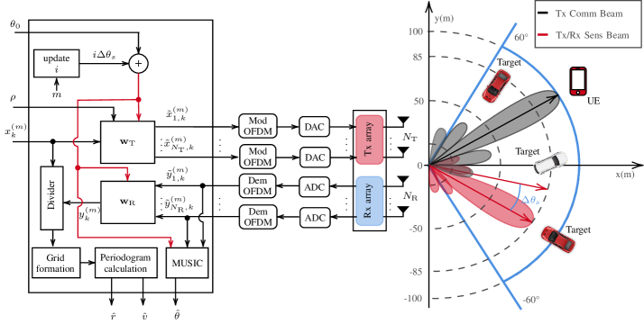
Figure 1: Block diagram of the 5G NR-based sensor with multibeam capability for joint communication and sensing.

As depicted in Fig. 1, a multiple antennas OFDM system is considered. The JSC system consists of a transmitter (Tx) antenna array with $N_{\mathrm{T}}$ elements and of an receiver (Rx) antenna array with $N_{\mathrm{R}}$ elements, used for communication and sensing, respectively. For both Tx and Rx we assume a uniform linear array (ULA) with half-wavelength separation, i.e., $d=\lambda/2$ with $\lambda=c/f_{\mathrm{c}}$, $c$ the speed of light, and $f_{\mathrm{c}}$ the carrier frequency. The communication system transmits a 5G NR waveform with $M$ OFDM symbols and $K$ active subcarriers to a UE in the cell [35]. The equivalent low-pass (ELP) representation of the signal transmitted by the $n$th antenna can be written as

$$s_{n}(t)=\sum_{m=0}^{M-1}\left(\sum_{k=0}^{K-1}\tilde{x}_{n,k}^{(m)}e^{j2\pi\frac{k}{T}t}\right)g(t-mT_{\mathrm{s}})$$ (1)

where $\tilde{x}_{n,k}^{(m)}$ is the modulation symbol, taken from a complex modulation alphabet, to be transmitted to the UE at the $m\text{th}$ OFDM symbol and $k\text{th}$ subcarrier, mapped through digital precoding at the $n\text{th}$ transmitting antenna, $g(t)$ is the employed pulse, $\Delta f=1/T$ is the subcarrier spacing, and $T_{\mathrm{s}}$ is the OFDM symbol duration including the cyclic prefix (CP).

II-A Joint waveform

The vector $\tilde{\mathbf{x}}_{k}^{(m)}\in\mathbb{C}^{N_{\mathrm{T}}\times 1}$ is defined as $\tilde{\mathbf{x}}_{k}^{(m)}=\mathbf{w}_{\mathrm{T}}x_{k}^{(m)}$, where $\mathbf{w}_{\mathrm{T}}\in\mathbb{C}^{N_{\mathrm{T}}\times 1}$ is the precoder vector used to map each modulation symbol, $x_{k}^{(m)}$, to the transmitting antennas. In particular, we consider a multibeam system where the power of the OFDM signal to be transmitted is split between communication and sensing, namely, the total available power is in part exploited to sense the environment and in part directed to the UE [12, 34]. Therefore, the transmitting beamformer (BF) vector $\mathbf{w}_{\mathrm{T}}$ can be written as [12]

$$\mathbf{w}_{\mathrm{T}}=\sqrt{\rho}\,\mathbf{w}_{\mathrm{T,s}}+\sqrt{1-\rho}\,\mathbf{w}_{\mathrm{T,c}}$$ (2)

where $\rho\in[0,1]$ is the parameter used to control the fraction of the total power apportioned to the two directions, while $\mathbf{w}_{\mathrm{T,c}}$ and $\mathbf{w}_{\mathrm{T,s}}$ are the communication and the sensing BF vectors, respectively. The latter are defined as [35]

$$\mathbf{w}_{\mathrm{T,c}}=\frac{\sqrt{P_{\mathrm{T}}G_{\mathrm{T}}^{\mathrm{a}}}}{N_{\mathrm{T}}}\,\mathbf{a}_{\mathrm{T}}^{c}(\theta_{\mathrm{T,c}})\quad$$ (3)

$$\mathbf{w}_{\mathrm{T,s}}=\frac{\sqrt{P_{\mathrm{T}}G_{\mathrm{T}}^{\mathrm{a}}}}{N_{\mathrm{T}}}\,\mathbf{a}_{\mathrm{T}}^{c}(\theta_{\mathrm{T,s}})$$ (4)

where $G_{\mathrm{T}}^{\mathrm{a}}$ is the transmit array gain along the beam steering direction (where such a gain is maximum), $P_{\mathrm{T}}G_{\mathrm{T}}^{\mathrm{a}}$ is the effective isotropic radiated power (EIRP), $\mathbf{a}_{\mathrm{T}}(\theta_{\mathrm{T,c}})\in\mathbb{C}^{N_{\mathrm{T}}\times 1}$ and $\mathbf{a}_{\mathrm{T}}(\theta_{\mathrm{T,s}})\in\mathbb{C}^{N_{\mathrm{T}}\times 1}$ are the steering vectors for communication and sensing, respectively. The spatial steering vector for a ULA at a given DoA/ direction of departure (DoD) $\theta_{l}$ is [36, Chapter 9],[35, Chapter 5]

$$\mathbf{a}(\theta_{l})=\left[1,e^{j2\pi d\sin(\theta_{l})/\lambda},\dots,e^{j2\pi(N_{\mathrm{a}}-1)d\sin(\theta_{l})/\lambda}\right]^{T}$$ (5)

where $N_{\mathrm{a}}$ is the number of array antenna elements. Since a half-wavelength separation is considered, the expression (5) reduces to

$$\mathbf{a}(\theta_{l})=[1,e^{j\pi\sin(\theta_{l})},\dots,e^{j\pi(N_{\mathrm{a}}-1)\sin(\theta_{l})}]^{T}.$$ (6)

Looking at (2), it is evident the trade-off between the performance of the communication and sensing functions. To guarantee certain sensing capabilities, it is necessary to reserve a fraction of the total power available for it, with a consequent reduction in communication coverage. To study how the communication system coverage changes by varying the EIRP, some metrics can be used according to the 3GPP Technical Report in [37]. In particular, maximum coupling loss (MCL), maximum path loss (MPL) and maximum isotropic loss (MIL) are the metrics used in 5G NR systems to express the coverage of the communication system [37, 38]. These metrics differ for some terms, but they share the main idea of maximum loss that the communication system can tolerate and still be operational. In particular, differently from MCL, MIL and MPL include also the antenna gains. Moreover, the MIL metric takes into account parameters such as shadow fading and penetration margins. A detailed analysis of this metric is out of the scope of this paper, but it is important to highlight that the fraction of power $\rho$ reserved for sensing results in a reduction of MPL and MIL by a factor $10\text{log}_{10}(\rho)\,$dB.

II-B Received signal

The vector $\mathbf{\tilde{y}}_{k}^{(m)}\in\mathbb{C}^{N_{\mathrm{R}}\times 1}$ of the received modulation symbols at each antenna after the fast Fourier transform (FFT) block in the OFDM receiver, is given by

$$\tilde{\mathbf{y}}_{k}^{(m)}=\mathbf{H}_{k}^{(m)}\tilde{\mathbf{x}}_{k}^{(m)}+\tilde{\boldsymbol{\nu}}_{k}^{(m)}+\tilde{\mathbf{n}}_{k}$$ (7)

where $\mathbf{H}_{k}^{(m)}\in\mathbb{C}^{N_{\mathrm{R}}\times N_{\mathrm{T}}}$ is the channel matrix for the $m$th OFDM symbol and the $k$th subcarrier, $\tilde{\boldsymbol{\nu}}_{k}^{(m)}\in\mathbb{C}^{N_{\mathrm{R}}\times 1}$ is the vector whose elements represent the self interference (SI) due to imperfect Tx–Rx isolation at each receiving antenna, and $\tilde{\mathbf{n}}_{k}\in\mathbb{C}^{N_{\mathrm{R}}\times 1}$ is the additive white Gaussian noise (AWGN) vector whose entries are independent, identically distributed (i.i.d.) random variables, having circularly symmetric zero mean Gaussian distribution with variance $\sigma_{\mathrm{N}}^{2}$.

Considering $L$ point target reflections, the channel matrix can be written as

$$\mathbf{H}_{k}^{(m)}=\sum_{l=1}^{L}\underbrace{\alpha_{l}e^{j2\pi mT_{\mathrm{s}}f_{\mathrm{D},l}}e^{-j2\pi k\Delta f\tau_{l}}}_{\triangleq\beta_{l}}\mathbf{a}_{\mathrm{R}}(\theta_{l})\mathbf{a}^{T}_{\mathrm{T}}(\theta_{l})$$ (8)

where $\tau_{l}$, $f_{\mathrm{D},l}$, and $\theta_{l}$ are the round-trip delay, the Doppler shift, and the DoA of the $l$th target, respectively. The term $\alpha_{l}=\left|\alpha_{l}\right|e^{j\phi_{l}}$ is the complex amplitude which includes phase shift and attenuation along the $l$th propagation path. The array response vector at the receiver for sensing is denoted in (8) by $\mathbf{a}_{\mathrm{R}}(\theta_{l})$. To simplify the presentation of the DoA estimation method, (8) can be recast in the more compact form

$$\mathbf{H}_{k}^{(m)}=\mathbf{A}_{\mathrm{R}}(\boldsymbol{\theta})\boldsymbol{\Sigma}\mathbf{A}_{\mathrm{T}}^{T}(\boldsymbol{\theta})$$ (9)

where $\mathbf{A}_{\mathrm{R}}(\boldsymbol{\theta})=[\mathbf{a}_{\mathrm{R}}(\theta_{1}),\dots,\mathbf{a}_{\mathrm{R}}(\theta_{L})]\in\mathbb{C}^{N_{\mathrm{R}}\times L}$ and $\mathbf{A}_{\mathrm{T}}(\boldsymbol{\theta})=[\mathbf{a}_{\mathrm{T}}(\theta_{1}),\dots,\mathbf{a}_{\mathrm{T}}(\theta_{L})]\in\mathbb{C}^{N_{\mathrm{T}}\times L}$ are the steering matrices for the targets’ directions $\boldsymbol{\theta}=[\theta_{1},\theta_{2},\dots,\theta_{L}]$, and $\boldsymbol{\Sigma}=\operatorname{diag}(\beta_{1},\beta_{2},\dots,\beta_{L})\in\mathbb{C}^{L\times L}$ is the diagonal matrix of the channel coefficients.

For what concerns the SI term, $\tilde{\boldsymbol{\nu}}_{k}^{(m)}$, in (7), each element $n$ of this vector can be considered as the signal scattered by a static target with an almost null distance from the receiver, i.e., with $f_{\mathrm{D,SI}}=0$ and $\tau_{\mathrm{SI}}=0$, thus it can be written as $\tilde{\nu}_{n,k}^{(m)}=\alpha_{\mathrm{SI},n}x_{k}^{(m)}$, where $\alpha_{\mathrm{SI},n}=\left|\alpha_{\mathrm{SI},n}\right|e^{j\phi_{\mathrm{SI},n}}$ is the complex amplitude, which includes phase shift and attenuation of the SI contribution at the $n$th receiving antenna element [39, 6]. As for the targets, all the attenuation factors $\alpha_{\mathrm{SI},n}$ are assumed to be the same for all the receiving antennas. Therefore, the signal-to-self interference ratio (SSIR) for the eco generated by the target $l$ at each receiving antenna is given by

$$\mathrm{SSIR}=\frac{|\alpha_{l}|^{2}}{|\alpha_{\mathrm{SI}}|^{2}}.$$ (10)

Starting from (7), by performing spatial combining through the receiving BF vector, $\mathbf{w}_{\mathrm{R}}=\mathbf{a}_{\mathrm{R}}^{c}(\theta_{\mathrm{R,s}})$, we have the received symbol $y_{k}^{(m)}=\mathbf{w}_{\mathrm{R}}^{T}\tilde{\mathbf{y}}_{k}^{(m)}$, which, using (9), can be expressed as

$$y_{k}^{(m)}=\mathbf{w}_{\mathrm{R}}^{T}\mathbf{A}_{\mathrm{R}}(\boldsymbol{\theta})\boldsymbol{\Sigma}\mathbf{A}_{\mathrm{T}}^{T}(\boldsymbol{\theta})\tilde{\mathbf{x}}_{k}^{(m)}+\mathbf{w}_{\mathrm{R}}^{T}\tilde{\boldsymbol{\nu}}_{k}^{(m)}+\mathbf{w}_{\mathrm{R}}^{T}\tilde{\mathbf{n}}_{k}.$$ (11)

II-C Beam-scanning

As mentioned above, the considered system is a multibeam JSC scheme, with a beam pointing to the UE and a beam pointing sequentially to different directions to sense the environment.

Referring to Fig. 1, during a scan the DoD and the DoA for sensing are the same. Specifically, we have

$$\theta_{\mathrm{T,s}}=\theta_{\mathrm{R,s}}=\theta_{0}+i\,\Delta\theta_{\mathrm{s}}\qquad i=0,\dots,N_{\mathrm{dir}}-1$$ (12)

where $\theta_{0}$ is the starting scan direction, $\Delta\theta_{\mathrm{s}}$ is the scan angle step, $i$ is the index used to update the direction, and $N_{\mathrm{dir}}$ is the number of directions explored to perform a complete scan from $-\theta_{0}$ to $\theta_{0}$. For each sensing direction, a number of OFDM symbols $M_{\mathrm{s}}<M$ is acquired from the receiver system. Therefore, since a 5G NR frame with $M$ symbols lasts $T_{\mathrm{f}}=10$ ms, by fixing $N_{\mathrm{dir}}$ it is possible to determine the number of frames and the time required to complete a scan as:

$$N_{\mathrm{f}}=\left\lceil\frac{M_{\mathrm{s}}N_{\mathrm{dir}}}{M}\right\rceil,\qquad T_{\mathrm{scan}}=T_{\mathrm{f}}N_{\mathrm{f}}.$$ (13)

The OFDM symbols collected in each direction are used to estimate range, Doppler and DoA of the target.

II-D Sensor-target-sensor path

In LOS propagation conditions the power received at a given array element from the $l$th path, illuminated by the sensing beam, is proportional to $|\alpha_{l}|^{2}$ and given by [36]

$$P_{\mathrm{R},l}=\rho\cdot\frac{P_{\mathrm{T}}G_{\mathrm{T}}^{\mathrm{a}}G_{\mathrm{R}}c^{2}\sigma_{\mathrm{RCS},l}}{(4\pi)^{3}f_{\mathrm{c}}^{2}d_{l}^{4}}\cdot\gamma_{l}$$ (14)

where $\sigma_{\mathrm{RCS},l}$ is the radar cross-section (RCS) of the point target $l$, $d_{l}$ is the distance between the $l$th target and the BS, $G_{\mathrm{R}}$ is the single element antenna gain at RX, and $\gamma_{l}=|\mathrm{AF}(\theta_{\mathrm{T,s}}-\theta_{l})|^{2}\in[0,1]$ where $\mathrm{AF}(\theta)$ is the normalized array factor at Tx that considers the non-perfect alignment between the target DoA and the sensing direction [40]; when $\theta_{l}=\theta_{\mathrm{T,s}}$ then $\gamma_{l}=1$. The signal-to-noise ratio (SNR) at the single receiving antenna element related to the $l$th target is defined as

$$\text{SNR}_{l}=\frac{P_{\mathrm{R},l}}{N_{0}K\Delta f}$$ (15)

where $P_{\mathrm{R},l}$, the received power from the $l$th path, is given in (14), and $N_{0}$ is the one-sided noise power spectral density (PSD) at each antenna element. When convenient, by normalizing the received symbols after the FFT in the OFDM receiver as $\mathbb{E}\{\lvert\tilde{y}_{n,k}^{(m)}\rvert^{2}\}=1$, (15) reduces to $\text{SNR}_{l}=1/\sigma_{\mathrm{N}}^{2}$.

III Estimation of Target Parameters and Detection

This section introduces MUltiple SIgnal Classification (MUSIC) for DoA estimation and periodogram-based frequency estimation for range and velocity evaluation. The estimation methods are performed for each sensing beam step in which $M_{\mathrm{s}}$ OFDM symbols are collected. To simplify the notation, we drop the scan index $i$.

III-A Estimation of the number of targets and DoAs

DoA estimation is performed by MUSIC that requires knowledge of the noise subspace, which in turn needs the number of targets to be known. Noise subspace can be identified via the covariance matrix of the received vector (7) $\mathbf{R}=\mathbb{E}\bigl{\{}\tilde{\mathbf{y}}_{k}^{(m)}\tilde{\mathbf{y}}_{k}^{(m){\dagger}}\bigr{\}}\in\mathbb{C}^{N_{\mathrm{R}}\times N_{\mathrm{R}}}$. In fact, since the noise is zero mean and independent of the target echoes, it follows that the $N_{\mathrm{R}}-L$ smallest eigenvalues of $\mathbf{R}$ are all equal to the noise power $\sigma_{\mathrm{N}}^{2}$ and the corresponding eigenvectors identify the noise subspace. Since the covariance matrix is not known a priori, the sample covariance matrix (SCM) can be used instead [32]. It is given by

$$\widehat{\mathbf{R}}=\frac{1}{KM_{\mathrm{s}}}\sum_{m=0}^{M_{\mathrm{s}}-1}\sum_{k=0}^{K-1}\tilde{\mathbf{y}}_{k}^{(m)}\tilde{\mathbf{y}}_{k}^{(m){\dagger}}.$$ (16)

The number of sources (target echoes in our scenario) can be estimated by model order selection based on information theoretic criteria [41, 42]. The approach starts by performing eigenvalue decomposition of the SCM of the observed vectors, $\widehat{\mathbf{R}}=\mathbf{U}\boldsymbol{\Lambda}\mathbf{U}^{\dagger}$, where the columns of $\mathbf{U}\in\mathbb{C}^{N_{\mathrm{R}}\times N_{\mathrm{R}}}$ are the eigenvectors and $\boldsymbol{\Lambda}=\mathrm{diag}(\lambda_{1},\dots,\lambda_{N_{\mathrm{R}}})$ is a diagonal matrix with eigenvalues sorted in descending order, i.e., $\lambda_{1}\geq\lambda_{2}\geq\dots\geq\lambda_{N_{\mathrm{R}}}$. Using the minimum description length (MDL) criterion, the estimated number of targets (considering that we are illuminating only targets within the sensing beam in the $i$th direction) is

$$L_{\mathrm{m}}=\!\!\operatorname*{arg\,min}_{s\in\{0,\dots,N_{\mathrm{R}}-1\}}\!\!\{\textrm{MDL}(s)\}$$ (17)

with

$$\begin{split}\textrm{MDL}(s)&=-\ln\left(\frac{\prod_{i=s+1}^{N_{\mathrm{R}}}\lambda_{i}^{1/(N_{\mathrm{R}}-s)}}{\frac{1}{N_{\mathrm{R}}-s}\sum_{i=s+1}^{N_{\mathrm{R}}}\lambda_{i}}\right)^{\!\!\!(N_{\mathrm{R}}-s)KM_{\mathrm{s}}}\\ &+\frac{1}{2}s(2N_{\mathrm{R}}-s)\ln(KM_{\mathrm{s}}).\end{split}$$ (18)

The MUSIC algorithm then starts from $\widetilde{\mathbf{U}}\in\mathbb{C}^{N_{\mathrm{R}}\times(N_{\mathrm{R}}-L_{\mathrm{m}})}$, the submatrix containing the $N_{\mathrm{R}}-L_{\mathrm{m}}$ eigenvectors corresponding to the smallest eigenvalues, $\lambda_{L_{\mathrm{m}}+1},\dots,\lambda_{N_{\mathrm{R}}}$, where such eigenvectors represent a good approximation of the noise subspace. Next, the pseudo-spectrum function, whose peaks reveal the presence of incoming signals, can be obtained as [43]

$$f_{\mathrm{m}}(\theta)=\frac{1}{\bigl{\|}\widetilde{\mathbf{U}}^{\dagger}\mathbf{a}(\theta)\bigr{\|}_{2}^{2}}.$$ (19)

The peak locations in $f_{\mathrm{m}}(\theta)$ are the DoA estimates $\widehat{\theta}$. However, as it will be better explained in Section V, in each sensing direction we search for a local maximum of (19) in a limited angle range $[\theta_{\mathrm{min}},\theta_{\mathrm{max}}]$, which depends on the beamwidth of the array response. The DoA estimate in each direction is thus given by

$$\widehat{\theta}=\operatorname*{arg\,max}_{\theta\in[\theta_{\mathrm{min}},\theta_{\mathrm{max}}]}\{f_{\mathrm{m}}(\theta)\}.$$ (20)

III-B Detection and range-Doppler estimation

For the range-Doppler profile evaluation, we start from the received symbols (11) from which, by expanding the matrix multiplications, we obtain

$$y_{k}^{(m)}=\left(\sum_{l=1}^{L}\beta_{l}\Upsilon(\theta_{\mathrm{T,s}},\theta_{\mathrm{R,s}},\theta_{l})\right)x_{k}^{(m)}+n_{k}$$ (21)

where $n_{k}=\mathbf{w}_{\mathrm{R}}^{T}\tilde{\mathbf{n}}_{k}$ and $\Upsilon(\theta_{\mathrm{T,s}},\theta_{\mathrm{R,s}},\theta_{l})\in\mathbb{C}$ is a factor which accounts for the gain due to the array response vector at Tx and Rx and the DoA of the target. Since the range and velocity of targets are embedded in $\beta_{l}$, first, a division is performed to remove the unwanted data symbols [44], i.e., $g_{k}^{(m)}=y_{k}^{(m)}/x_{k}^{(m)}$, which leads to

$$g_{k}^{(m)}=\sum_{l=1}^{L}\alpha_{l}e^{j2\pi mT_{\mathrm{s}}f_{\mathrm{D},l}}e^{-j2\pi k\Delta f\tau_{l}}\Upsilon(\theta_{\mathrm{T,s}},\theta_{\mathrm{R,s}},\theta_{l})+\nu_{k}$$ (22)

where $\nu_{k}=n_{k}/x_{k}^{(m)}$. Note that (22) contains, for each target, two complex sinusoids whose frequencies are related to $f_{\mathrm{D},l}$ and $\tau_{l}$, while $\alpha_{l}$ and $\Upsilon(\theta_{\mathrm{T,s}},\theta_{\mathrm{R,s}},\theta_{l})$ are constant terms.

Starting from (22), a periodogram can be computed in order to estimate range and speed of the target as [44, 45, 6]

$$\mathcal{P}(q,p)=\left|\sum_{k=0}^{K_{\mathrm{p}}-1}\biggl{(}\sum_{m=0}^{M_{\mathrm{p}}-1}g_{k}^{(m)}e^{-j2\pi\frac{mp}{M_{\mathrm{p}}}}\biggr{)}e^{j2\pi\frac{kq}{K_{\mathrm{p}}}}\right|^{2}$$ (23)

with $q=0,\dots,K_{\mathrm{p}}-1$ and $p=0,\dots,M_{\mathrm{p}}-1$, which consists of $K$ FFTs of length $M_{\mathrm{p}}$ and $M_{\mathrm{s}}$ inverse fast Fourier transforms of length $K_{\mathrm{p}}$. In this work, $K_{\mathrm{p}}>K$ is calculated as the next power of two of $K$, whereas $M_{\mathrm{p}}>M_{\mathrm{s}}$ is the next power of two of $F_{\mathrm{p}}\cdot M_{\mathrm{s}}$, where $F_{\mathrm{p}}$ is the zero-padding factor to improve speed estimation resolution.

The periodogram (23) represents the range-Doppler map from which the first operation performed is target detection by a hypothesis test between $H_{0}$, where only the noise is present, and $H_{1}$, which refers to the presence of the target, i.e.,

$$\mathcal{P}(q,p)\overset{H_{1}}{\underset{H_{0}}{\gtrless}}\eta.$$ (24)

The threshold $\eta$ is chosen to ensure a predefined false alarm probability $P_{\mathrm{FA}}$. When the sensing beamwidth is relatively small, only one target is likely to be present in a given sensing direction, and if the test (24) rejects the null hypothesis, it is easy to find the location of the peak in the periodogram

$$(\widehat{q},\widehat{p})=\operatorname*{arg\,max}_{(q,p)}\{\mathcal{P}(q,p)\}$$ (25)

and evaluate the distance and radial speed of the target as

$$\widehat{r}=\frac{\widehat{q}\,c}{2\Delta fK_{\mathrm{p}}},\qquad\widehat{v}=\frac{\widehat{p}\,c}{2f_{\mathrm{c}}T_{\mathrm{s}}M_{\mathrm{p}}}.$$ (26)

The distance and velocity resolutions are intrinsic characteristics of the periodogram and only depend on the 5G NR parameters, i.e., number of OFDM symbols, number of active subcarriers, subcarrier spacing, and OFDM symbol duration, and are given by [44, Chapter 3]

$$\Delta r=\frac{c}{2\Delta fK_{\mathrm{p}}},\qquad\Delta v=\frac{c}{2f_{\mathrm{c}}T_{\mathrm{s}}M_{\mathrm{p}}}.$$ (27)

Algorithm 1 Pruning redundant target points

1:$\mathbf{Z}\leftarrow\mathbf{z}_{i}=[\widehat{r}_{i},\widehat{v}_{i},\mathcal{P}(\widehat{r}_{i},\widehat{v}_{i}),\widehat{\theta}_{i},f_{\mathrm{m}}(\widehat{\theta}_{i})]$

2:$\mathbf{Z_{\mathrm{sort}}}\leftarrow$ sort $\mathbf{Z}$ in decreasing order according to the $3$rd column

3:$\mathbf{z}_{\mathrm{prun},1}\leftarrow\mathbf{z}_{\mathrm{sort},1}$ $\triangleright$ copy first row of $\mathbf{Z}_{\mathrm{sort}}$ in $\mathbf{Z}_{\mathrm{prun}}$

4:$k\leftarrow 1$ $\triangleright$ initialize row index of $\mathbf{Z}_{\mathrm{prun}}$

5:for $i=2:N_{\mathrm{max}}$ do

6:     $\mathrm{count}\leftarrow 0$

7:     for $j=1:k$ do

8:         if $\widehat{r}_{\mathrm{prun},j}-\epsilon_{\mathrm{r}}\leq\widehat{r}_{\mathrm{sort},i}\leq\widehat{r}_{\mathrm{prun},j}+\epsilon_{\mathrm{r}}$ and

9:          $\widehat{v}_{\mathrm{prun},j}-\epsilon_{\mathrm{v}}\leq\widehat{v}_{\mathrm{sort},i}\leq\widehat{v}_{\mathrm{prun},j}+\epsilon_{\mathrm{v}}$ then

10:              $\mathrm{count}\leftarrow\mathrm{count}+1$

11:              break

12:         end if

13:     end for

14:     if $\mathrm{count}=0$ then

15:         $k\leftarrow k+1$ $\triangleright$ update row index of $\mathbf{Z}_{\mathrm{prun}}$

16:         $\mathbf{z}_{\mathrm{prun},k}\leftarrow\mathbf{z}_{\mathrm{sort},i}$

17:     end if

18:end for

19:$\widehat{L}\leftarrow k$

Output: $\mathbf{Z}_{\mathrm{prun}}$ and its number of rows, $\widehat{L}$

III-C Pruning redundant target points

As explained above, the considered JSC system searches for a peak in the pseudo-spectrum (19) and in the periodogram (23) for each sensing direction for which the test (24) chooses the hypothesis $H_{1}$. When a target is detected in a particular direction, it might be detected also in some adjacent directions when the periodogram $\mathcal{P}$ is above threshold because of the beam sidelobes. These detected points are originated by the same target and are characterized by inaccurate DoA estimates. As it will be better quantified in Section V, this effect is due to the choice of searching the maximum of MUSIC pseudo-spectrum in a limited range, as in (20), that reduces the computational cost of searching but may yield multiple detection points per target. To maintain the benefits of local search, we propose a method to thin out redundant target points (hereafter also referred to as repeated targets) that has proven effective.

First, all the collected peaks and estimates are organized in a matrix $\mathbf{Z}$, whose rows are the vectors

$$\mathbf{z}_{i}=\left[\widehat{r}_{i},\widehat{v}_{i},\mathcal{P}(\widehat{r}_{i},\widehat{v}_{i}),\widehat{\theta}_{i},f_{\mathrm{m}}(\widehat{\theta}_{i})\right]\quad i=1,\dots,N_{\mathrm{max}}$$ (28)

where $N_{\mathrm{max}}\leq N_{\mathrm{dir}}$ is the number of sensing directions in which the test (24) rejects the null hypothesis. Subsequently, these rows are sorted in descending order with respect to the values, $\mathcal{P}(\widehat{r}_{i},\widehat{v}_{i})$, to form a new matrix $\mathbf{Z}_{\mathrm{sort}}$. Finally, a check on the elements of $\mathbf{Z}_{\mathrm{sort}}$ is performed to remove redundant target points, i.e., those with very similar estimates of both distance and radial velocity (within a given range of uncertainty). This results in a new matrix $\mathbf{Z}_{\mathrm{prun}}$ with a number of rows $\widehat{L}\leq N_{\mathrm{max}}$. The sort operation ensures that only range and speed pairs associated with the largest values of the periodogram are kept between the repeated points. The whole procedure is detailed in Algorithm 1. As it can be seen, the definition of redundant target point is linked to the choice of two parameters, $\epsilon_{\mathrm{r}}$, and $\epsilon_{\mathrm{v}}$, that account for the measurement uncertainty. In particular, in the algorithm a target indexed with $i$ is considered a repetition of an already detected target denoted with $j$ if its estimated range, $\widehat{r}_{i}$, and velocity, $\widehat{v}_{i}$, meet the conditions, $\widehat{r}_{j}-\epsilon_{\mathrm{r}}\leq\widehat{r}_{i}\leq\widehat{r}_{j}+\epsilon_{\mathrm{r}}$, and $\widehat{v}_{j}-\epsilon_{\mathrm{v}}\leq\widehat{v}_{i}\leq\widehat{v}_{j}+\epsilon_{\mathrm{v}}$, respectively. The choice of the two parameters $\epsilon_{\mathrm{r}}$ and $\epsilon_{\mathrm{v}}$ will be discussed in Section V.

IV Performance Evaluation in the Presence of Multiple Targets

This section introduces the performance metric employed to address the concept of miss-distance, or error, in a multi-target system. In particular, when considering a multi-object system, a consistent metric should capture the difference between two sets of vectors (the truth and the estimated), not only in terms of localization error but also in terms of cardinality error. For this reason, in this work, the OSPA metric [46], [47] is used to study the performance of the considered JSC system in a multi-target scenario.

The OSPA metric is a miss-distance indicator, which summarizes in a unique measure the estimation accuracy in both the number and location of the targets. More precisely, given the true positions of the $L$ targets, $\mathbf{P}=\left[\mathbf{p}_{1},\dots,\mathbf{p}_{L}\right]$, with $\mathbf{p}_{l}=(x_{l},y_{l})=(r_{l}\cos{\theta_{l}},r_{l}\sin{\theta_{l}})$, and the $\widehat{L}$ estimates, $\widehat{\mathbf{P}}=\left[\widehat{\mathbf{p}}_{1},\dots,\widehat{\mathbf{p}}_{\widehat{L}}\right]$, the distance between an arbitrary pair of the estimate and the true position, cut off at $\bar{c}>0$, is defined as [46]

$$d^{(\bar{c})}\left(\mathbf{p},\widehat{\mathbf{p}}\right)=\min\left\{\bar{c},d\left(\mathbf{p},\widehat{\mathbf{p}}\right)\right\}$$ (29)

where $d\left(\mathbf{p},\widehat{\mathbf{p}}\right)=\bigl{\|}\mathbf{p}-\widehat{\mathbf{p}}\bigr{\|}_{2}$ is the Euclidean distance between the estimate and the true position, and $\bar{c}$ is the cutoff parameter that determines how the metric penalizes cardinality error with respect to the localization one. Denoting by $\Pi_{k}$ the set of permutations on $\{1,2,\dots,k\}$ for any $k\in\mathbb{N}$, for $1\leq q\leq\infty$ and $\bar{c}>0$, the OSPA metric of order $q$ and with cutoff $\bar{c}$ is defined as [46]

$$\begin{split}\bar{d}_{q}^{(\bar{c})}&\left(\mathbf{P},\widehat{\mathbf{P}}\right)=\\ &\left(\frac{1}{\widehat{L}}\left(\min_{\pi\in\Pi_{\widehat{L}}}\sum_{l=1}^{L}\left(d^{(\bar{c})}\left(\mathbf{p}_{l},\widehat{\mathbf{p}}_{\pi(l)}\right)\right)^{q}+\bar{c}^{q}(\widehat{L}-L)\right)\right)^{1/q}\end{split}$$ (30)

if $L\leq\widehat{L}$, and $\bar{d}_{q}^{(\bar{c})}\left(\mathbf{P},\widehat{\mathbf{P}}\right)=\bar{d}_{q}^{(\bar{c})}\left(\widehat{\mathbf{P}},\mathbf{P}\right)$ if $L>\widehat{L}$. Essentially, for $L\leq\widehat{L}$, the OSPA distance can be obtained by the following steps:

1. Find the $L$-elements subset of $\widehat{P}$ that has the shortest distance to $P$, corresponding to the optimal subset assignment;

2. If a point $\widehat{\mathbf{p}}_{n}\in\widehat{\mathbf{P}}$ is not paired with any point in $\mathbf{P}$, let $d_{n}=\bar{c}$; otherwise, $d_{n}$ is the minimum value between $\bar{c}$ and the distance between the two points in a pair;

3. The OSPA distance is given by $\bar{d}_{q}^{(\bar{c})}\left(\mathbf{P},\widehat{\mathbf{P}}\right)=\left(\left(\sum_{l=1}^{L}d_{n}^{q}\right)/\widehat{L}\right)^{1/q}$.

The OSPA distance can be interpreted as a $q$th order per-target error for a multi-object scenario. The metric can be divided into two components, one accounting for localization error and the other for cardinality error. In particular, for $q<\infty$ these components are given by [46]

$$\begin{split}\bar{e}_{q,\mathrm{loc}}^{(\bar{c})}(\mathbf{P},\widehat{\mathbf{P}})=&\left(\frac{1}{\widehat{L}}\min_{\pi\in\Pi_{\widehat{L}}}\sum_{l=1}^{L}\left(d^{(\bar{c})}\left(\mathbf{p}_{l},\widehat{\mathbf{p}}_{\pi(l)}\right)\right)^{q}\right)^{1/q},\\ \bar{e}_{q,\mathrm{card}}^{(\bar{c})}(\mathbf{P},\widehat{\mathbf{P}})=&\left(\frac{\bar{c}^{q}(\widehat{L}-L)}{\widehat{L}}\right)^{1/q}\end{split}$$ (31)

TABLE I: JSC system parameters

5G specification $\rightarrow$	NR 100	NR 400
$f_{\mathrm{c}}$ [GHz]	3.5	28
$\Delta f$ [kHz]	30	120
Active subcarriers $K$	3276	3168
OFDM symbols per frame $M$	280	1120
OFDM symbols per direction $M_{\mathrm{s}}$	112	112
Number of antennas $N_{\mathrm{T}}=N_{\mathrm{R}}$	10	10 50 100
Array beamwidth $\Delta\Theta$ [°]	27	27 5.3 2.6

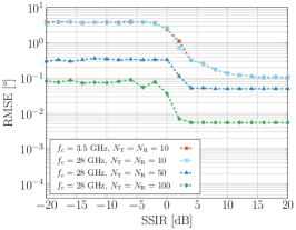
(a)

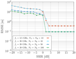
(b)

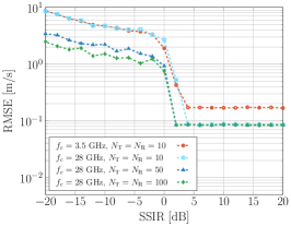
(c)

Figure 2: Sensing performance as a function of the SSIR for DoA, distance, and speed estimates, when $\text{SNR}=-20\,$dB.

if $L\leq\widehat{L}$, and $\bar{e}_{q,\mathrm{loc}}^{(\bar{c})}(\mathbf{P},\widehat{\mathbf{P}})=\bar{e}_{q,\mathrm{loc}}^{(\bar{c})}(\widehat{\mathbf{P}},\mathbf{P})$, $\bar{e}_{q,\mathrm{card}}^{(\bar{c})}(\mathbf{P},\widehat{\mathbf{P}})=\bar{e}_{q,\mathrm{card}}^{(\bar{c})}(\widehat{\mathbf{P}},\mathbf{P})$ if $L>\widehat{L}$.

In the metric, the value of $q$ determines the sensitivity of the $\bar{d}_{q}^{(\bar{c})}$ to outlier estimates, while $\bar{c}$ balances the cardinality error component with respect to the localization one, as a part of the total error. As $\bar{c}$ decreases, the localization error becomes dominant compared with the cardinality error, whereas larger values of $\bar{c}$ emphasize the latter. The best choice for $\bar{c}$ to maintain a balance between the two components is any value significantly larger than a typical localization error, but significantly smaller than the maximum distance between objects.

V System-Level Analysis

System level analysis is carried out through numerical simulations to evaluate the performance of the above-described JSC scheme. For all the simulations, 5G NR signals compliant with 3GPP Technical Specification in [48] are considered. The main 5G NR parameters employed for the generation of the standardized signals are summarized in Table I. In addition, a quadrature phase shift keying (QPSK) modulation alphabet is used for the generation of the OFDM signal. As it can be seen in Fig. 1, the considered system scans the environment in the range $[-\theta_{0},\theta_{0}]$, with $\theta_{0}=-60$°, and a step $\Delta\theta_{\mathrm{s}}$. The choice of $N_{\mathrm{dir}}$, and so of $\Delta\theta_{\mathrm{s}}$, mainly depends on the beamwidth $\Delta\Theta$ of the array response (here referred to $-10\,\text{dB}$ gain with respect to the beam direction) reported in Table I. As expected, when the number of antennas decreases, $\Delta\Theta$ becomes larger, and a lower $N_{\mathrm{dir}}$ is necessary to avoid blind zones. Once $N_{\mathrm{dir}}$ is chosen, the number of necessary 5G NR frames, and consequently, the total time needed to complete a scan cycle, are calculated from (13). For each selected direction, the periodogram is obtained from $K$ active subcarriers, which differ between 5G numerologies, and a fixed number of OFDM symbols $M_{\mathrm{s}}=112$, with $F_{\mathrm{p}}=10$, required to perform speed estimation. Furthermore, for what concerns the DoA estimation algorithm, the MUSIC pseudo-spectrum (19) is computed only in the range $\left[\theta_{\mathrm{R,s}}-\Delta\Theta/2,\theta_{\mathrm{R,s}}+\Delta\Theta/2\right]$, to reduce the processing time and the position error.

As already stated in Section II, this work addresses the performance analysis of a JSC multibeam system considering two different scenarios, single-target, and multi-target. For the former, the primary purpose of the analysis is to derive the RMSE of position and speed of the target. When deriving the RMSE as a function of the SNR, the target is considered aligned with the sensing beam (i.e., $\gamma=1$) and the noise variance is $\sigma_{\mathrm{N}}^{2}=1/\text{SNR}$, as mentioned in Section II-D. Whereas when the RMSE is evaluated varying the distance of the target, the SNR is computed using (15) and the following system parameters are considered: the target has an RCS equal to $\sigma_{\mathrm{RCS}}=1\,\text{m}^{2}$, the EIRP is set to $P_{\mathrm{T}}G_{\mathrm{T}}^{\mathrm{a}}=43\,\text{dBm}$, $G_{\mathrm{R}}=1$, and the noise PSD is $N_{0}=k_{\mathrm{B}}T_{0}F$ where $k_{\mathrm{B}}=1.38\cdot 10^{-23}\,\text{JK}^{-1}$ is the Boltzmann constant, $T_{0}=290\,$K is the reference temperature, and $F=10\,$dB is the receiver noise figure. The number of Monte Carlo (MC) iterations for each SNR or distance value is $N_{\mathrm{MC}}=2000$. For the multi-object scenario, we consider $L=10$ point targets, one of which is the UE, and the same system parameters as the single-target scenario. Two different values of the fraction of power devoted to sensing, $\rho=0.1$ and $\rho=0.3$, a carrier frequency equal to $f_{c}=28\,\text{GHz}$, and $N_{\mathrm{T}}=N_{\mathrm{R}}=50$ antennas, are considered. In this set of results, the OSPA metric, presented in Section IV, is the performance indicator to summarize the effectiveness of the designed system. The OSPA metric is computed for $q=2$, as recommended by [46], and $\bar{c}=10\,$m to guarantee a good balance between localization and cardinality error.

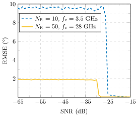
(a)

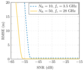
(b)

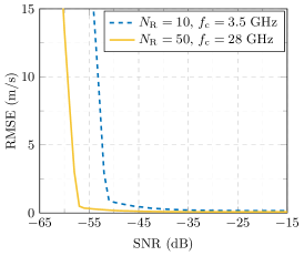
(c)

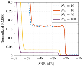
(d)

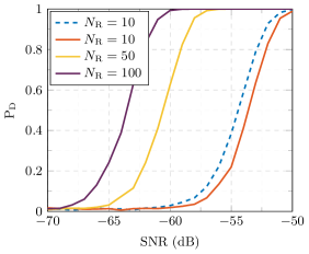
(e)

Figure 3: Sensing performance as a function of the SNR for distance, DoA, speed, and position estimates, and detection probability. The dashed lines represent the results at $f_{\mathrm{c}}=3.5\,$GHz, whereas the continuous lines represent the results at $f_{c}=28\,$GHz. In particular, (a), (b) and (c) show the RMSE results when the MIMO system consists of $N_{\mathrm{T}}=N_{\mathrm{R}}=10$ antennas at $f_{\mathrm{c}}=3.5\,$GHz, and $N_{\mathrm{T}}=N_{\mathrm{R}}=50$ antennas at $f_{\mathrm{c}}=28\,$GHz, whereas (d) and (e) depict the normalized localization error and the detection probability for different number of antennas.

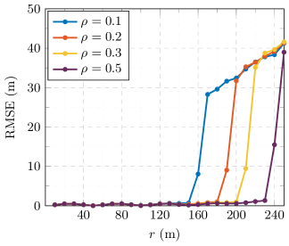
(a)

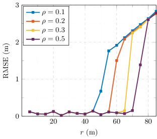
(b)

Figure 4: Target localization performance as a function of the sensor-target distance varying the fraction of power $\rho$ reserved for sensing. Note that the maximum range of $250\,$m at $3.5\,$GHz and $85\,$m at $28\,$GHz is within the maximum unambiguous range for the respective numerology detailed in Table I [44].

As it will be explained in the following, we will start investigating the impact of SI on estimation performance, focusing on the RMSE of DoA, distance, and speed estimates by varying the SSIR introduced in Section II-B.

V-A RMSE and detection probability vs SNR and SSIR

Let us start analyzing the SI issue. Fig. 2 shows the RMSE of DoA, range, and radial speed estimates obtained when only a single target is present and $\mathrm{SNR}=-20\,\text{dB}$, by varying the SSIR for different 5G NR parameters and number of antennas. As it can be noticed, the system performance quickly degrades for low SSIR values, but when $\mathrm{SSIR}\geq 10\,$dB, the RMSE of DoA, range, and radial speed estimates, reaches a floor where thermal noise is the only limiting factor. Therefore, if proper SI suppression can be performed, either through beamforming optimization or through digital cancellation techniques [6, 32], the estimation error can be kept low.
From now on, an analysis of the RMSE by varying the SNR is performed considering SI negligible. In particular, the SNR is varied from $-65$ to $-15\,\text{dB}$, while distance, speed, and DoA of the target are varied randomly, from one iteration to another, with a uniform distribution from $20$ to $85\,\text{m}$, $-20$ to $20\,\text{m/s}$, and $-60^{\circ}$ to $60^{\circ}$, respectively. In Fig. 3, the results obtained for the RMSE of distance, angle, speed, and position are shown. As the periodogram used to estimate speed and radial distance of the target is computed on the symbols obtained after spatial combining, the whole estimation process is subject to a double processing gain, one resulting from the periodogram calculation, equal to $10\log_{10}(K\cdot M_{\mathrm{s}})\,$dB [49], and the other from the beamforming gain, equal to $10\log_{10}(N_{\mathrm{R}})\,$dB. For this reason, the MIMO system can estimate range and speed with high accuracy for SNR significantly lower than those reached by the DoA estimation algorithm, as it can be seen in Fig. LABEL:figure_a, Fig. LABEL:figure_b, and Fig. LABEL:figure_c. In fact, MUSIC is not subject to any processing gain, and the RMSE of angle estimation starts to increase at much higher SNR values, depending on the number of receiving antennas, $N_{\mathrm{R}}$. In particular, for increasingly negative values of SNR, the RMSE (in degree) vs SNR curves converge approximately to $\Delta\Theta/2.8$, because of the limited search interval, $\Delta\Theta$, over which the pseudo-spectrum is computed. As previously stated, $\Delta\Theta$, and consequently the upper bound value of the curves, strictly depends on the number of antennas, as it can be noticed comparing the blue dashed line and continuous yellow line curves in Fig. LABEL:figure_a, Fig. LABEL:figure_b and Fig. LABEL:figure_c.

From the estimated range, $\widehat{r}$, and DoA, $\widehat{\theta}$, the position estimate of the target is $\widehat{\mathbf{p}}=(\widehat{x},\widehat{y})=(\widehat{r}\cos{\widehat{\theta}},\widehat{r}\sin{\widehat{\theta}})$. The normalized RMSE, shown in Fig. LABEL:figure_d, is derived from the Euclidean distance between the estimated position, $\widehat{\mathbf{p}}$, and the true location of the target, $\mathbf{p}=(x,y)=(r\cos{\theta},r\sin{\theta})$, divided by the true distance, $r$, as

$$\text{Normalized \acs{RMSE}}=\sqrt{\frac{1}{N_{\mathrm{MC}}}\sum_{j=1}^{N_{\mathrm{i}}}{\frac{\bigl{\|}{\widehat{\mathbf{p}}}_{j}-{\mathbf{p}}_{j}\bigr{\|}_{2}^{2}}{r_{j}^{2}}}}.$$ (32)

The normalization in (32) eliminates the dependency of the position RMSE on the distance generalizing the results. In fact, since the length of the chord of a circumference is directly proportional to its radius, the DoA error causes the position error to increase with distance. In Fig. LABEL:figure_d the position estimate dependency on the DoA is emphasized for different numbers of antennas and 5G numerologies. As the SNR decreases, it is possible to notice the impact of DoA, which causes a first drop in the performance, and the effect of range estimation error, which leads to a second performance drop at lower SNR.

Another important parameter in sensing is the detection probability $P_{\mathrm{D}}$ as a function of the SNR as shown in Fig. LABEL:figure_e. In these plots, the threshold $\eta$ has been chosen to ensure a $P_{\mathrm{FA}}=1\%$. As expected, since detection is performed on the range-Doppler map, the same map used for velocity and range estimation, it is easy to notice that the range and velocity estimation start degrading when detection probability degrades. Therefore, the main factor limiting the radar performance is DoA estimation.

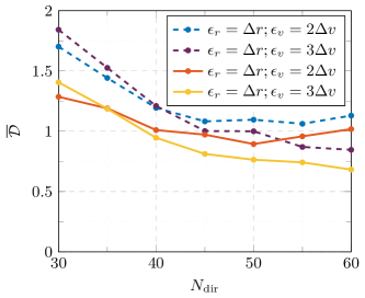
(a)

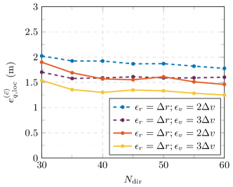
(b)

Figure 5: Mean cardinality error (a) and mean OSPA localization error (b) varying the number of sensing directions, $N_{\mathrm{dir}}$, for a JSC system with $f_{\mathrm{c}}=28$GHz, $N_{\mathrm{T}}=N_{\mathrm{R}}=50$, obtained with $N_{\mathrm{MC}}=500$ Monte Carlo iterations. Dashed lines represent the result for $\rho=0.1$, whereas the continuous lines represent the results for $\rho=0.3$.

V-B RMSE vs distance

Let us now analyze the trade-off between communication and sensing varying $\rho$ in (2). As it can be observed in Fig. LABEL:figure_3a and LABEL:figure_3b, the system works well also for moderately low values of $\rho$, e.g., $\rho=0.1$. Notably, the position RMSE is below $0.33\,$m and $0.1\,$m, at $3.5\,\text{GHz}$ and $28\,\text{GHz}$, respectively, even at tens of meters (in LOS condition). It is also important to highlight that the RMSE values reached at $3.5\,\text{GHz}$ are much higher than that at $28\,\text{GHz}$. This mainly depends on the larger $\Delta\Theta$ resulting from $N_{\mathrm{T}}=N_{\mathrm{R}}=10$, with respect to the beamwidth with $N_{\mathrm{T}}=N_{\mathrm{R}}=50$ antennas. Moreover, at the considered ranges, the RMSE of the position mainly depends on DoA estimation error, and when this error reaches the upper bound, the position RMSE becomes proportional to the distance, $r$, as previously explained in Section V-A.

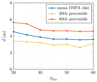
(a)

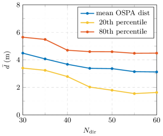
(b)

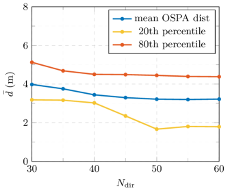
(c)

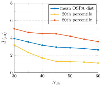
(d)

Figure 6: Mean value, $20$th and $80$th percentile of the OSPA distance varying the number of sensing directions for different values of $\epsilon_{r}$, $\epsilon_{v}$ and $\rho$, with $f_{\mathrm{c}}=28\,$GHz and $N_{\mathrm{T}}=N_{\mathrm{R}}=50$. The OSPA metric is computed for $\bar{c}=10\,$m and $q=2$. The considered values are: $\epsilon_{r}=\Delta r$ and $\epsilon_{v}=2\Delta v$ with $\rho=0.1$ (a) and $\rho=0.3$ (c), $\epsilon_{r}=\Delta r$ and $\epsilon_{v}=3\Delta v$ with $\rho=0.1$ (b) and $\rho=0.3$ (d).

V-C Performance analysis of multi-target scenario

For the multi-object scenario analysis let us consider $L=10$ point targets ($9+1$ UE). Each target is associated with an SNR that depends on its radial distance from the monostatic sensor, on its RCS, and on the alignment between the target and the sensing direction, in accordance with (15). Without loss of generality let us assume all the targets with the same RCS, equal to $\sigma_{\mathrm{RCS}}=1\,\text{m}^{2}$, as in Section V-B. The number of MC iterations for this group of results is set to $N_{\mathrm{MC}}=500$. In each MC iteration targets positions are randomly generated according to a uniform distribution within a sector with radial distance between $20$ to $85\,\text{m}$ and angle from $-60^{\circ}$ to $60^{\circ}$.

The primary purpose of this analysis is to study the performance of the considered JSC system when multiple targets are present, computing the OSPA metric introduced in Section IV for different choices of $N_{\mathrm{dir}}$, ranging from $30$ to $60$ sensing directions. In particular, one of the main objectives is to study the influence of the uncertainty parameters, $\epsilon_{r}$ and $\epsilon_{v}$, used in the repeated targets pruning algorithm presented in Section III-C, and of the parameters $\rho$, on the detection and localization capabilities of the system.

For what concerns $\epsilon_{r}$ and $\epsilon_{v}$, a good choice consists of using a multiple of distance and velocity resolutions, $\Delta r$ and $\Delta v$, defined in (27). In fact, due to the presence of AWGN, radial distance and velocity estimates of a repeated target may fall in adjacent bins of the periodogram with respect to those of the original target. In this sense, between range and velocity, it is the latter that presents greater RMSE in the low SNR regime; this is due to zero padding, which increases velocity resolution at the expense of sensitivity to noise. The mean cardinality error is used to choose these parameters. This metric is given by

$$\mathcal{\overline{D}}=\frac{1}{N_{\mathrm{MC}}}\sum_{i=1}^{N_{\mathrm{MC}}}|L-\widehat{L}|.$$ (33)

Importantly, this metric does not distinguish between miss-detection, false alarm, and repeated target; however, it can be considered a good indicator for analyzing the average performance of the considered algorithm. In fact, fixing the system parameters, miss-detection and false alarm rates can be regarded as approximately constant, so if $\mathcal{\overline{D}}$ decreases, that should be caused by a drop in the targets’ repetition rate. Fig. 5 shows the mean cardinality error and the mean OSPA localization error computed varying the number of sensing directions, $N_{\mathrm{dir}}$, for different values of $\epsilon_{r}$, $\epsilon_{v}$ and $\rho$. As it can clearly be noticed, by fixing $\epsilon_{r}$ and $\epsilon_{v}$, the overall performance of the system (both in localization and cardinality error) improves for increasing values of $\rho$. For what concerns the localization error, the results shown in Fig. LABEL:fig:loc_err are in agreement with those presented in Fig. LABEL:figure_3b. As the position of the target is varied between $20$ and $85\,\text{m}$, the system performance is worse for $\rho=0.1$ than $\rho=0.3$, as expected. In Fig. LABEL:fig:card_err it is possible to notice as for $N_{\mathrm{dir}}\geq 40$ the mean cardinality error becomes smaller choosing $\epsilon_{v}=3\Delta v$, both for $\rho=0.3$ and $\rho=0.1$, and, in particular, for $\rho=0.3$ the system on average misses less than one target. As pointed out, a value of $\epsilon_{r}>\Delta r$ does not change appreciably the system performance; therefore, its value is kept fixed, letting $\epsilon_{v}$ vary. This latter term most affects the repeated targets pruning algorithm detection performance due to zero padding, as already observed.

In Fig. 6, the mean OSPA metric is computed varying $N_{\mathrm{dir}}$ for the same values of $\epsilon_{r}$, $\epsilon_{v}$ and $\rho$ used above. In addition, the $20$th and $80$th percentile are shown to better understand the range of values the OSPA metric can assume for different positions of the targets. Also in this case, the best performance are obtained for $\rho=0.3$, $\epsilon_{r}=\Delta r$ and $\epsilon_{v}=3\Delta v$. In particular, for this choice of parameters the mean value of $\bar{d}$ is below $3\,\text{m}$ and the $20$th percentile is approximately equal to $1\,\text{m}$ for $N_{\mathrm{dir}}=60$. Note, however, that such numerical results also consider the portion of the monitored area where the DoA estimation is severely degraded (see Fig. 4); a proper sensing cell sizing may avoid such region and lead to much better performance.

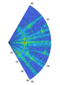
(a)

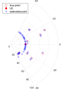
(b)

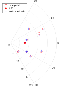
(c)

Figure 7: Considered scenario with $9$ targets and $1$ UE. The range-angle map in (a) has been obtained with $f_{\mathrm{c}}=28\,\text{GHz}$, $N_{\mathrm{T}}=N_{\mathrm{R}}=50$ antennas, $N_{\mathrm{dir}}=60$ and $\rho=0.3$. (b) shows the point detected starting from the range-angle map in (a), before repeated targets pruning. In (c) the result obtained after the removal of the repeated targets, performed with $\epsilon_{r}=\Delta r$ and $\epsilon_{v}=3\Delta v$ is shown.

As a final system-level analysis, in Fig. 7 an example of multiple targets map returned by the JSC sensor is shown. The parameters are $\rho=0.3$, $\epsilon_{r}=\Delta r$ and $\epsilon_{v}=3\Delta v$. First, in Fig. LABEL:fig:range_angle_map the range-angle map obtained by computing the periodogram (23) in each sensing direction, is shown. Then, in Fig. LABEL:fig:range_angle_points1 we have the targets detected through the hypothesis test (24), and the resulting range estimates (25)-(26) and angle estimates (20). As it can be seen, multiple points per target are present. After the repeated targets pruning algorithm introduced in Section III-C the resulting targets are shown in Fig. LABEL:fig:range_angle_points2. As we can observe, in this particular case the algorithm is very effective in removing all redundant points while retaining all the useful points. As expected, most of the repeated points are on the circumference with a radius equal to the distance between the UE and the monostatic sensor; this is to be attributed to a large fraction of power used for the communication beam which illuminates the UE causing a strong received echo.

VI Conclusion

In this work, we designed a multibeam system for JSC based on 5G NR, capable of detecting and locating multiple targets. We provided a system-level analysis and proposed an algorithm for pruning phantom targets that arise as a consequence of beam-scanning in the presence of beam sidelobes. We identified the main dominant factors affecting performance and compared two system setups operating at sub-$6\,$GHz, and mmWave frequencies. The findings of this paper have demonstrated that: $i)$ DoA estimation is the primary source of error when used to evaluate the target position; $ii)$ even with a relatively small fraction of power devoted to sensing, good localization performance at tens of meters can be achieved in LOS even at mmWave: $iii)$ in the sub-$6\,$GHz band targets can be detected at higher distances but with lower accuracy mainly because of the reduced number of antenna elements; $iv)$ Tens of targets can be detected and localized with sub-meter level accuracy when the power for sensing is capable of ensuring reliable DoA estimation.

References

- [1] L. Pucci, E. Matricardi, E. Paolini, W. Xu, and A. Giorgetti, “Performance analysis of joint sensing and communication based on 5G New Radio,” in IEEE Work. on Adv. in Netw. Loc. and Nav. (ANLN), Globecom 2021, Madrid, Spain, Dec. 2021.
- [2] M. Chiani, A. Giorgetti, and E. Paolini, “Sensor radar for object tracking,” Proc. IEEE, vol. 106, no. 6, pp. 1022–1041, June 2018.
- [3] B. Paul, A. R. Chiriyath, and D. W. Bliss, “Survey of RF communications and sensing convergence research,” IEEE Access, vol. 5, pp. 252–270, 2016.
- [4] F. Liu, C. Masouros, A. P. Petropulu, H. Griffiths, and L. Hanzo, “Joint radar and communication design: Applications, state-of-the-art, and the road ahead,” IEEE Trans. Commun., vol. 68, no. 6, pp. 3834–3862, Feb. 2020.
- [5] C. B. Barneto, L. Anttila, M. Fleischer, and M. Valkama, “OFDM radar with LTE waveform: Processing and performance,” in 2019 IEEE Radio and Wireless Symposium (RWS), Orlando, FL, USA, Jan. 2019, pp. 1–4.
- [6] C. B. Barneto, T. Riihonen, M. Turunen, L. Anttila, M. Fleischer, K. Stadius, J. Ryynänen, and M. Valkama, “Full-duplex OFDM radar with LTE and 5G NR waveforms: challenges, solutions, and measurements,” IEEE Trans. Microw. Theory Tech., vol. 67, no. 10, pp. 4042–4054, Oct. 2019.
- [7] A. Evers and J. A. Jackson, “Analysis of an LTE waveform for radar applications,” in 2014 IEEE Radar Conference, Cincinnati, OH, USA, May 2014, pp. 0200–0205.
- [8] S. Bartoletti, A. Conti, and M. Z. Win, “Passive radar via LTE signals of opportunity,” in Proc. 2014 IEEE International Conference on Communications Workshops (ICC), Sydney, Australia, June 2014, pp. 181–185.
- [9] C. R. Berger, B. Demissie, J. Heckenbach, P. Willett, and S. Zhou, “Signal processing for passive radar using OFDM waveforms,” IEEE J. Sel. Topics Signal Process., vol. 4, no. 1, pp. 226–238, Feb. 2010.
- [10] M. L. Rahman, J. A. Zhang, X. Huang, Y. J. Guo, and R. W. Heath, “Framework for a perceptive mobile network using joint communication and radar sensing,” IEEE Trans. Aerosp. Electron. Syst., vol. 56, no. 3, pp. 1926–1941, 2020.
- [11] J. A. Zhang, M. L. Rahman, K. Wu, X. Huang, Y. J. Guo, S. Chen, and J. Yuan, “Enabling joint communication and radar sensing in mobile networks – a survey,” 2021.
- [12] J. A. Zhang, X. Huang, Y. J. Guo, J. Yuan, and R. W. Heath, “Multibeam for joint communication and radar sensing using steerable analog antenna arrays,” IEEE Trans. Veh. Technol., vol. 68, no. 1, pp. 671–685, Jan. 2019.
- [13] P. Kumari, J. Choi, N. González-Prelcic, and R. W. Heath, “IEEE 802.11ad-based radar: An approach to joint vehicular communication-radar system,” IEEE Trans. Veh. Technol., vol. 67, no. 4, pp. 3012–3027, 2018.
- [14] R. C. Daniels, E. R. Yeh, and R. W. Heath, “Forward collision vehicular radar with IEEE 802.11: Feasibility demonstration through measurements,” IEEE Trans. Veh. Technol., vol. 67, no. 2, pp. 1404–1416, 2018.
- [15] Y. Luo, J. A. Zhang, X. Huang, W. Ni, and J. Pan, “Optimization and quantization of multibeam beamforming vector for joint communication and radio sensing,” IEEE Trans. Commun., vol. 67, no. 9, pp. 6468–6482, 2019.
- [16] ——, “Multibeam optimization for joint communication and radio sensing using analog antenna arrays,” IEEE Trans. Veh. Technol., vol. 69, no. 10, pp. 11 000–11 013, 2020.
- [17] V. Petrov, G. Fodor, J. Kokkoniemi, D. Moltchanov, J. Lehtomaki, S. Andreev, Y. Koucheryavy, M. Juntti, and M. Valkama, “On unified vehicular communications and radar sensing in millimeter-wave and low terahertz bands,” IEEE Trans. Wireless Commun., vol. 26, no. 3, pp. 146–153, 2019.
- [18] F. Liu, L. Zhou, C. Masouros, A. Li, W. Luo, and A. Petropulu, “Toward dual-functional radar-communication systems: Optimal waveform design,” IEEE Trans. Signal Process., vol. 66, no. 16, pp. 4264–4279, 2018.
- [19] F. Liu, C. Masouros, A. Li, H. Sun, and L. Hanzo, “Mu-mimo communications with mimo radar: From co-existence to joint transmission,” IEEE Trans. Wireless Commun., vol. 17, no. 4, pp. 2755–2770, 2018.
- [20] R. M. Gutierrez, H. Yu, A. R. Chiriyath, G. Gubash, A. Herschfelt, and D. W. Bliss, “Joint sensing and communications multiple-access system design and experimental characterization,” in 2019 IEEE Aerospace Conference, Big Sky, MT, USA, Mar. 2019, pp. 1–8.
- [21] J. A. Zhang, A. Cantoni, X. Huang, Y. J. Guo, and R. W. Heath, “Framework for an innovative perceptive mobile network using joint communication and sensing,” in 2017 IEEE 85th Vehicular Technology Conference (VTC Spring), Sydney, NSW, Australia, June 2017, pp. 1–5.
- [22] J. A. Zhang, X. Huang, Y. J. Guo, and M. L. Rahman, “Signal stripping based sensing parameter estimation in perceptive mobile networks,” in 2017 IEEE-APS Top. Conf. Antennas Propag. Wirel. Commun. (APWC), Verona, Italy, Sept. 2017, pp. 67–70.
- [23] M. L. Rahman, J. A. Zhang, X. Huang, and Y. J. Quo, “Analog antenna array based sensing in perceptive mobile networks,” in 2017 IEEE-APS Top. Conf. Antennas Propag. Wirel. Commun. (APWC), Verona, Italy, Sept. 2017, pp. 199–202.
- [24] M. L. Rahman, P.-f. Cui, J. A. Zhang, X. Huang, Y. J. Guo, and Z. Lu, “Joint communication and radar sensing in 5G mobile network by compressive sensing,” in 2019 19th International Symposium on Communications and Information Technologies (ISCIT), Ho Chi Minh City, Vietnam, Sept. 2019, pp. 599–604.
- [25] K. V. Mishra, M. Bhavani Shankar, V. Koivunen, B. Ottersten, and S. A. Vorobyov, “Toward millimeter-wave joint radar communications: A signal processing perspective,” IEEE Signal Process. Mag., vol. 36, no. 5, pp. 100–114, 2019.
- [26] J. A. Zhang, A. Cantoni, X. Huang, Y. J. Guo, and R. W. Heath, “Joint communications and sensing using two steerable analog antenna arrays,” in 2017 IEEE 85th Vehicular Technology Conference (VTC Spring), Sydney, NSW, Australia, June 2017, pp. 1–5.
- [27] M. Alloulah and H. Huang, “Future millimeter-wave indoor systems: A blueprint for joint communication and sensing,” Computer, vol. 52, no. 7, pp. 16–24, 2019.
- [28] F. Liu and C. Masouros, “Hybrid beamforming with sub-arrayed mimo radar: Enabling joint sensing and communication at mmwave band,” in ICASSP 2019 - 2019 IEEE Int. Conf. Acoust. Speech Signal Process. (ICASSP), Brighton, UK, May 2019, pp. 7770–7774.
- [29] P. Kumari, S. A. Vorobyov, and R. W. Heath, “Adaptive virtual waveform design for millimeter-wave joint communication–radar,” IEEE Trans. Signal Process., vol. 68, pp. 715–730, 2020.
- [30] S. H. Dokhanchi, B. S. Mysore, K. V. Mishra, and B. Ottersten, “A mmWave automotive joint radar-communications system,” IEEE Trans. Aerosp. Electron. Syst., vol. 55, no. 3, pp. 1241–1260, 2019.
- [31] M. Kiviranta, I. Moilanen, and J. Roivainen, “5G radar: Scenarios, numerology and simulations,” in Proc. Int. Conf. on Military Comm. and Inf. Sys. (ICMCIS), Budva, Montenegro, May 2019, pp. 1–6.
- [32] S. D. Liyanaarachchi, C. Baquero B., T. Riihonen, M. Heino, and M. Valkama, “Joint multi-user communication and MIMO radar through full-duplex hybrid beamforming,” in Proc. IEEE Int. Symp. on Joint Comm. & Sensing (JCS), online, Feb. 2021, pp. 1–5.
- [33] P. Kumari, M. E. Eltayeb, and R. W. Heath, “Sparsity-aware adaptive beamforming design for IEEE 802.11ad-based joint communication-radar,” in Proc. IEEE Radar Conf., Boston, MA, USA, Sep. 2018, pp. 923–928.
- [34] C. B. Barneto, S. D. Liyanaarachchi, T. Riihonen, L. Anttila, and M. Valkama, “Multibeam design for joint communication and sensing in 5G New Radio networks,” in Proc. IEEE Int. Conf. on Comm. (ICC), online, Jun. 2020, pp. 1–6.
- [35] H. Asplund, D. Astely, P. von Butovitsch, T. Chapman, M. Frenne, F. Ghasemzadeh, M. Hagström, B. Hogan, G. Jöngren, J. Karlsson et al., Advanced Antenna Systems for 5G Network Deployments: Bridging the Gap Between Theory and Practice. Academic Press, 2020.
- [36] M. A. Richards, Fundamentals of radar signal processing. McGraw-Hill, 2005.
- [37] Study on NR coverage enhancements, 3GPP TR 38.830, 12 2020, version 1.0.0 Release 17.
- [38] S. Moloudi, M. Mozaffari, S. N. K. Veedu, K. Kittichokechai, Y.-P. E. Wang, J. Bergman, and A. Höglund, “Coverage evaluation for 5G reduced capability new radio (NR-redcap),” IEEE Access, vol. 9, pp. 45 055–45 067, 2021.
- [39] Y. Zeng, Y. Ma, and S. Sun, “Joint radar-communication: Low complexity algorithm and self-interference cancellation,” in 2018 IEEE Global Communications Conference (GLOBECOM), 2018, pp. 1–7.
- [40] S. J. Orfanidis, Electromagnetic Waves and Antennas, 1st ed. New Jersey, USA: Sophocles J. Orfanidis, 2016.
- [41] M. Wax and T. Kailath, “Detection of signals by information theoretic criteria,” IEEE Trans. Acoust., Speech, Signal Process., vol. 33, pp. 387–392, Apr. 1985.
- [42] A. Mariani, A. Giorgetti, and M. Chiani, “Model order selection based on information theoretic criteria: Design of the penalty,” IEEE Trans. Signal Process., vol. 63, no. 11, pp. 2779–2789, Jun. 2015.
- [43] R. O. Schmidt, “Multiple emitter location and signal parameter estimation,” IEEE Trans. Antennas Propag., vol. 34, no. 3, pp. 276–280, Mar. 1986.
- [44] M. Braun, “OFDM radar algorithms in mobile communication networks,” Ph.D. dissertation, Karlsruhe Institute of Technology, 2014.
- [45] M. Braun, C. Sturm, and F. K. Jondral, “Maximum likelihood speed and distance estimation for OFDM radar,” in Proc. IEEE Radar Conf., Arlington, VA, USA, May 2010, pp. 256–261.
- [46] D. Schuhmacher, B.-T. Vo, and B.-N. Vo, “A consistent metric for performance evaluation of multi-object filters,” IEEE Trans. Signal Process., vol. 56, no. 8, pp. 3447–3457, Aug. 2008.
- [47] Z. Li, A. Giorgetti, and K. Sithamparanathan, “Multiple radio transmitter localization via UAV-based mapping,” IEEE Trans. Veh. Technol., pp. 1–12, 2021.
- [48] 5G; NR; Physical channels and modulation, 3GPP TS 38.211, 7 2020, version 16.2.0 Release 16.
- [49] C. Sturm and W. Wiesbeck, “Waveform design and signal processing aspects for fusion of wireless communications and radar sensing,” Proc. IEEE, vol. 99, no. 7, pp. 1236–1259, Jul. 2011.