Deep Networks for Image and Video Super-Resolution

1 Abstract

Efficiency of gradient propagation in intermediate layers of convolutional neural networks is of key importance for super-resolution task. To this end, we propose a deep architecture for single image super-resolution (SISR), which is built using efficient convolutional units we refer to as mixed-dense connection blocks (MDCB). The design of MDCB combines the strengths of both residual and dense connection strategies, while overcoming their limitations. To enable super-resolution for multiple factors, we propose a scale-recurrent framework which reutilizes the filters learnt for lower scale factors recursively for higher factors. This leads to improved performance and promotes parametric efficiency for higher factors. We train two versions of our network to enhance complementary image qualities using different loss configurations. We further employ our network for video super-resolution task, where our network learns to aggregate information from multiple frames and maintain spatio-temporal consistency. The proposed networks lead to qualitative and quantitative improvements over state-of-the-art techniques on image and video super-resolution benchmarks.

2 Introduction

Single image super-resolution (SISR) aims to estimate a high-resolution (HR) image from a low-resolution (LR) input image, and is an ill-posed problem. Due to its diverse applicability starting from surveillance to medical diagnosis, and from remote sensing to HDTV, the SISR problem has gathered substantial attention from computer vision and image processing community. The ill-posed nature of the problem is generally addressed by learning a LR-HR mapping function in a constrained environment using example HR-LR patch pairs.

One way is to learn a mapping function that linearly correlates the HR-LR patch pairs. Such linear functions can be easily learned with few example images as has been practiced by some SR approaches [1, 2, 3]. But, linear mapping between such patch pairs may not be representative enough to learn different complex structures present in the image. The mapping function would benefit from learning non-linear relationships between HR-LR patch pairs. Recent convolutional neural network (CNN) based models are quite efficient for such a purpose, and can be useful in extracting relevant features by making deeper models. However, deeper models often face vanishing/exploding gradient issues, which can be partially mitigated by using residual mapping [4, 5]. Deep residual models has been employed for higher level vision tasks, where batch normalization is generally used for a useful class-specific normalized representation. However, such representation is not much useful in low-level vision task such as SR [6]. Most deep CNN based SR models do not make full use of the hierarchical features from the original LR images. Thus, the scope of improvement in performance is there in effective employment of the hierarchical features from all the convolutional layers, as has been employed by a residual dense network [7] using a sequence of residual dense blocks (RDBs). However, most of these deep networks require huge number of parameters, which becomes a bottleneck in the situation where limited computational resources are available.

Further, most of the networks need to be trained separately for different scale factors. This issue can be addressed by jointly training the model for different scale factors, as has been performed by VDSR [8]. Moreover, VDSR requires bicubic interpolated version of the LR image as an input. Processing interpolated images precludes the model from learning direct LR-HR feature mapping. Additionally, passing the high-resolution image and feature-maps through a large number of layers increases the memory consumption as well as computational requirements. Another way to consider multiple scale factors is to train a network jointly for different factors by including scale-specific features [6]. However, these techniques produce sub-optimal results for higher scale factors like $8$.

Motivated by the performances of residual connections and dense connections, we propose a deep architecture for single image super-resolution (SISR) that consists of efficient convolutional units, which we entitle as mixed-dense connection blocks (MDCB). MDCB combines the advantages of residual and dense connections while subduing their limitations. The combination improves the flow of information through the network, alleviating the gradient vanishing problem. In addition, it allows the reuse of feature maps from preceding layers, avoiding the re-learning of redundant features. In order to master our network for super-resolving different scale factors, we make use of weight transfer strategy via scale-recurrent framework. Intuitively, filters learnt for smaller scale factors can be transfered to higher-ones. Sharing of parameters across scales is crucial for efficiently super-resolving by higher up-sampling factors. Our scale recurrence framework built using MDCBs is parametrically more efficient than most of the existing works, enabling our strategy to work with limited resources.

It has been recently found that a result with good RMSE value often fails to satisfy perceptually, and the converse also holds true  [9]. Thus, to obtain photo-realistic results, we employ a GAN framework with deep feature loss (VGG) function in the network, which leads to a second network. These two networks enable us to traverse along the perception-distortion curve. The first network is trained to produce an output with better RMSE score, whereas the second one tries to produce result with better perceptual score. Different weighting schemes of GAN and VGG and pixel reconstruction losses enables us to traverse along the perception distortion curve [9] and can be used to reach a desirable trade-off between the two.

We have further employed our network for the task of video SR, where our model super-resolves each frame by aggregating HR information from a local temporal window of LR frames. We demonstrate that the proposed SR framework can approximate the inverted image formation process, while maintaining spatio-temporal consistency and the estimated HR frames are good candidates for representing the ground truth frames of a video. The proposed networks help in achieving better qualitative and quantitative performance against the state-of-the-art techniques on image and video super-resolution benchmarks.

3 Related Works and Contributions

We address the problems of SR for single image and extend it to video. To discuss the related works for each of the problems, we discuss this section mainly in two parts, corresponding to the single image and video SR. In each category, there are numerous approaches starting from conventional to deep learning based. Though, our technique is based on deep learning, we also brief some of the conventional techniques for completeness.

3.1 Works on Single Image SR

Super resolving single image generally requires some example HR images to import relevant information for generating the HR image. Two stream of approaches make use of the HR example images in their frameworks: i) Conventional approaches, and ii) deep learning based approaches.

3.1.1 Conventional Single Image SR

Conventionally, single image SR approaches work by finding out patches similar to the target patch in the database of patches, extracted from example images. However, the possibility of many similarities along with the imaging blur, and noise often makes the problem ill-posed. Different prior information help in address the ill-posed nature of the problem [10, 11, 12, 13, 14, 15, 16, 17, 18].

Natural images are generally piecewise smooth, hence it is often incorporated as prior knowledge by means of Tikhonov, total variation, Markov random field, etc. [19, 20, 21]. Image patches tend to repeat in the image non-locally, and can provide useful information in terms of non-local prior to super-resolve an image [22, 2, 23, 3]. The redundancy present in an image indicates sparsity in some domain, and can be employed in SR framework by employing sparsity inducing norm. Here, the assumption is that a target patch can be represented by combining few patches from the database linearly[1, 24, 2, 3]. Different priors can be combined to provide various information to the framework. For example, sparsity inducing norm can be combined with non-local similarity to improve the SR performance [25, 3].

Although, the sparsity based prior works quite efficiently, the linear mapping of information fails to represent complex structures of image. Here, deep-learning based approaches behave better through non-linear mapping of HR information [26, 27, 28, 8, 29, 30, 31, 32, 33, 6, 34, 35].

3.1.2 Deep Learning Based Single Image SR

Deep learning stepped into the field of SR via SRCNN [36], which extends the concept of sparse representation using CNN. CNNs typically contains large number of filters along with series of non-linearities and hence are a better candidate for representing complex input-output mapping than the conventional approaches, and are shown to yield superior results. However, increasing the depth of such architecture increase difficulty in training. Introducing residual connections into the framework along with skip connections and/or recursive convolutions are known to make it less cumbersome. Following such methodologies, VDSR [8] and DRCN [37] have demonstrated performance improvement. The power of recursive blocks involving residual units to create a deeper network is explored in [29]. Recursive unit in conjunction with gate unit acts as a memory unit that adaptively combines the previous states with the current state to produce a super resolved image [33]. However, these approaches interpolate the LR image to the HR grid before feeding it to the network. This technique increases the computational requirement since all the convolution operations are then performed on high-resolution feature-maps. To alleviate this computational burden, networks have been tailored to extract features from the LR image through a series of layers. Towards the end of such networks, up-sampling process is performed to match with the HR dimension [27, 5]. This process can be made faster by reducing the dimension of the features going to the layers that maps from LR to HR, and is known as FSRCNN [27].

Recent studies show that traditional metrics used to measure image restoration quality do not correlate with perceptual quality of the result. The work of in SRResNet [5] utilized ResNet [4] based network with adversarial training framework (GAN) [38] with perceptual loss [39] to produce photo-realistic HR results. The perceptual loss is further used with texture synthesis mechanism in GAN based framework to improve SR performance [32]. Though these approaches are able to add textures in the image, sometimes the results contain artifacts. The model architecture of SRResNet [5] is further simplified and optimized to achieve further improvements in EDSR [6]. This is further modified in MDSR [6], which performs joint training for different scale factors by introducing scale-specific feature extraction and pixel-shuffle layers, while keeping rest of the layers common.

3.2 Works on Video SR

We briefly discuss some of the related works on video SR including conventional approaches and recent deep learning based approaches.

3.2.1 Conventional Approaches

The seminal work of [40] has enabled various development in multi-frame SR. Motion between the consecutive frames can be employed in reconstruction based methods [41, 42, 43]. The quality of the super-resolved video depends on the accuracy of motion estimation of pixels. In order to maintain the continuity of the result, a back-projection method was introduced to minimize reconstruction error iteratively [44]. Example-based image SR approaches cannot be directly extended for video by super-resolving each frame separately. Independent processing of frames can give rise to flickering artifacts among the frames. This issue can be mitigated by introducing smoothness prior among the frames [45]. Different spatial-temporal resolutions of frames can also be combined to super-resolve a video [46], where a dictionary has been constructed by using scene specific HR images captured by a still camera. Single image SR has also been exercised for video SR in frame by frame basis by incorporating inverted image formation process [47].

The accurate motion estimation requirement for video SR has been relaxed by multidimensional kernel regression [48]. Here each pixel is approximated by 3D local series, whose coefficients are estimated by solving a least-square problem, where weights were introduced based on 3D space-time orientation in the pixel neighborhood [48]. However, this method still assumes the blur kernel that was involved in the LR image formation model. To do away with the assumptions of blur kernel along with motion and noise level a Bayesian strategy has been developed [49], where the degradation parameters are estimated from the given image sequence. Motion blur due to relative motion between camera and object can be handled by considering the least blurred pixels through an EM framework [50].

3.2.2 Deep Learning Based Approaches

The motion information among the frames has been explored by BRCN [51], which modeled long-term contextual information of frames using recurrent neural networks. Three types of convolutions (feed-forward, recurrent, and conditional) were involved to meet with requirement of spatial dependency, long-term temporal and contextual dependencies. However, iterative motion estimation procedure increases the computational burden. To reduce the computing load, DECN [52] introduced non-iterative framework, where different hand-crafted optical flow algorithms are used to generate different SR versions, which were finally combined using a deep network. Similar technique was employed in VSRnet [53], where motion was compensated in the LR frames by using an optical flow algorithm. The pre-processed LR frames were sent to a pre-trained deep network to generate the final result. Real-time estimation of motions among the input LR frames was tried out by VESPCN [54], which is an end-to-end deep network that extracts the optical flow by warping frames using a spatial transformer [55]. Here, the HR frames are produced by another deep network.

Motion estimation and compensation has been practiced in many video SR approaches. However, Liu et al. [56] have demonstrated that adaptive usage of the motion information in various temporal radius of a temporal adaptive neural network can produce better results. Several inference branches were used for each temporal radius. The resultant images from these branches are assembled to produce the final result [56]. The motion compensation module of VESPCN [54] was employed in [57], where sub-pixel motion compensation layer was introduced to perform simultaneous motion compensation and resolution enhancement. After the motion compensation, the frames are super-resolved using an encoder-decoder framework with skip connections [58] and ConvLSTM [59] module for faster convergence as well as to take care of the sequential nature of video. Previous end-to-end CNN based video SR methods have focused on explicit motion estimation and compensation to better re-construct HR frames. Unlike the previous works, our approach does not require explicit motion estimation and compensation steps.

4 Architecture Design

Success of recent approaches has emphasized the importance of network design. Specifically, the most recent image and video SR approaches are built upon two popular image classification networks: residual networks [4] and densely connected networks [60]. These two network designs have also enjoyed success and achieved state-of-the-art performance in other image restoration tasks such as image denoising, dehazing and deblurring. Motivated by the generalization capability of such advances in network designs, our work explores further improvements in network engineering which enable efficient extraction of high-resolution features from low-resolution images.

4.1 Proposed Architecture

The effectiveness of residual and dense connections has been proved via the significant success in various vision tasks yet, they cannot be considered as the optimum topology. For example, too many additions on the same feature space may impede the information flow in ResNet [60], and there may be the same type of raw features from different layers, which leads to a certain redundancy in DenseNet. Recent works of [61, 62] partially addressed these issues and demonstrate improvement in image classification performance. However, very few works have explored optimal network topologies for low-level vision tasks (e.g., image and video SR). We build upon the understanding of dense-topology to design a network for the task of super-resolution that benefits from a mixture of such connections and term it as Mixed-Dense Connection Network (MDCN).

Our MDCN not only achieves higher accuracy but also enjoys higher parameter efficiency than the state-of-the-art SR approaches. Its strength lies in its building blocks called Mixed-Dense Connection Blocks (MDCBs) which contain a rich set of connections to enable efficient feature-extraction and ease the gradient propagation. Inclusion of addition and concatenation based connections improves classification accuracy, and is more effective than going deeper or wider, given an option to increase the capacity of the network. In each MDCB, $n$ Dual Link Units are present. Additive links in the unit grant the benefits of reusing common features with low redundancy, while concatenation links give the network more flexibility in learning new features. Although additive link is flexible with their positions and sizes, each Dual Link Unit performs the additive operation to the last F features of the input. Within each unit, the number of features for additive connections is $F$ and the concatenating connections is $K$. A visual depiction of these connections can be seen in the Fig. 1(a). This unit adds $K$ new feature maps to the input. The number of features in the input to each MDCB is $F$ as shown in Fig. 1(b) and after $n$ units, the feature maps contains $F+n*K$ channels. The growth-rate $K$ of concatenation connections was shown to affect the image classification performance positively in [61, 62]. Further, it was experimentally demonstrated in [7] that deep networks containing many dense blocks stacked together are difficult to train for image restoration and result in poor performance. To handle this, we utilize a gating mechanism to allow larger growth rate by reducing the number of features and hence stabilizes the training of wide network. Each convolution or deconvolution layer is followed by a rectified linear unit (ReLU) for nonlinear mapping, except for the final $1\times 1$ layer.

In summary, the advantage of mixed-dense connections manifests in form of significant improvement in propagating error gradients during training. The block has two advantages: Firstly, existing feature channels get modified to learn the residuals: helping in deeper and hierarchical feature extraction. Secondly, feature concatenation with moderate growth-rate promotes new feature exploration. While having these advantages, it also handles the disadvantages: moderate growth rate leads to reduction of redundant features.

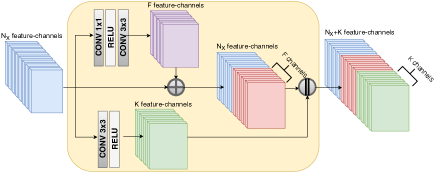
(a) Structure of our Dual Link unit. The first link selectively modifies $F$ existing feature-maps through addition, while the second link adds $K$ new features through concatenation.

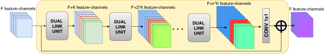
(b) Design of our mixed-dense connection block (MDCB). The features channels in red-shade correspond to the channels modified by the additive connection. The features channels in green-shade correspond to the channels added due to concatenation connection.

Figure 1: Structural details of our mixed-dense connection block (MDCB). Each block accepts the darker shade in the feature channels corresponds to deeper and rich features extracted from the initial feature map.

Our complete network (MDCN) broadly consists three parts: initial feature extraction module, a series of mixed-dense connection block (MDCBs) and an HR reconstruction module, as shown in Fig.2. Specifically, the feature extraction module contains two convolutional layers to extract basic feature-maps containing $F$ channels, which are fed to the first MDCB. The HR reconstruction module contains a convolution layer which takes $F$ chanenls features in LR space to $4*F$ channels. The pixel-shuffle layer accepts $4*F$ channels in LR space and returns $F$ channels in HR space, which are passed to the final conv layer to obtain the 3-channel HR image.
Initial upsampling: A few approaches interpolate the original LR image to the desired size to form the input to the network. This pre-processing step not only increases computation complexity, but also loses some details of the original LR image. Our network operates on the LR image, extracting deep hierarchical features from it and feeds them to a pixel-shuffle layer to result into the HR image features.
Filter Size: A large receptive field is important for utilizing spatial inter-dependencies in the structures present in the LR image. Since receptive-field of the network increases with network depth and/or filter size, depth of the network plays an crucial role in the super-resolution performance, as is evident from the existing state-of-the-art. A few initial works [26] did utilize larger filter size (larger than $3\times 3$) to compensate for smaller depth, but showed only limited super-resolving performance. This can be attributed to the superior speed and parametric efficiency of a $3\times 3$ filters above higher-size kernels. A stack of $3\times 3$ filters is capable of learning more complex mapping via the non-linearity and the composition of abstraction. Hence, we use $3\times 3$ filters for all the layers in our network.
Differences with [61],[62]: While [61] and [62] are proposed for a high-level computer vision task (object recognition), MDCN is suited for image restoration tasks and adopts the concept of blending a variety of dense topological connections at both macro and micro level. Other ncessary design changes include removal of the batch-normalization (BN) layers since they consume the same amount of GPU memory as convolutional layers, increase computational complexity, and hinder performance for image super-resolution. We also remove the pooling layers, since they could discard pixel-level information necessary for super-resolution. To enable higher growth rate, each MDCB contains with a $1\times 1$ convolution layer, which fuses the information from the large number of features channels into a fewer feature channels and feeds these to the next MDCB block. Further each MDCB contains a third connection in the form of an additive operation between its input features and the output features.

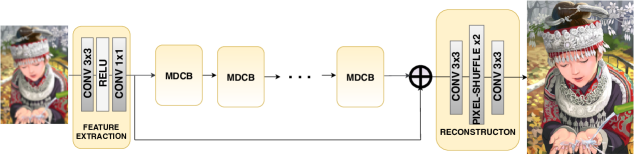
Figure 2: Architecture of our Mixed Dense Connection Network (MDCN).

4.2 Scale-Recurrent Design

Most existing SR algorithms treat super-resolution of different scale factors as independent problems without considering and utilizing mutual relationships among different scales in SR. Examples include EDSR [6], which require many scale-specific networks that need to be trained independently to deal with various scales. On the other hand, architectures like VDSR [8] can handle super-resolution of several scales jointly in the single network. Training the VDSR model with multiple scales boosts the performance and outperforms scale-specific training, implying the redundancy among scale-specific models. Nonetheless, VDSR style architecture takes bicubic interpolated image as the input, which contains less information (as compared to the true LR image) leading to sub-optimal feature extraction; and performs convolutions in HR space, leading to higher computation time and memory requirements.

We propose a scale-recurrent training scheme which has the advantages of the approaches mentioned above, while subduing their limitations. Our network’s global design is a multi-scale pyramid which recursively uses the same convolutional filters across the scales, motivated from the fact that a network capable of super-resolving an image by a factor of $2$ can be recursively used to super-resolve the image by a factor $2^{s}$, $s=2,3,\cdots$ Even with the same training data, the recurrent exploitation of shared weights works in a way similar to using data multiple times to learn parameters, which actually amounts to data augmentation regarding scales. We design the network to reconstruct HR images in intermediate steps by progressively performing a $2\times$ up-sampling of the input from the previous level. Specifically, we first train a network to perform SR by a factor of $2$ and then re-utilize the same weights to take the output of $2\times$ as input and result into a output at resolution $4\times$. This architecture is then fine-tuned to perform $4\times$ SR. We experimentally found that such initialization (training for task of $2\times$ SR) leads to better convergence of the networks for larger scale factor. Ours is the first approach that efficiently re-utilizes the parameters across scales, which significantly reduces the number of trainable parameters while yielding performance gains for higher scale factors. An illustration of this scheme is shown in Fig. 3.

Figure 3: Scale-Recurrent utilization of our Mixed Dense Connection Network (MDCN). Output of $2\times$ network is fed recursively for $4\times$ and $8\times$ super-resolution.

5 Experimental Results on Single Image SR

Here, we evaluate our approach on standard datasets for different scale-factors. After discussing different experimental settings, we illustrate the results of our network, and compare them quantitatively as well as qualitatively with state-of-the-art approaches. The section concludes by meeting with the perception-distortion trade-off.

5.1 Settings

We next indicate the experimental settings about datasets, degradation models, training settings, implementation details, and evaluation metrics.

• Datasets and degradation model: Following [63, 6, 7, 34], we use 800 training images from DIV2K dataset [63] as training set. For testing, we use five standard benchmark datasets: Set5 [64], Set14 [24], B100 [65], Urban100 [35], and Manga109 [66]. We have considered bicubic interpolation for generating LR images, corresponding to the HR examples.

• Training settings and implementation details: Network’s number of filters are chosen to reduce the number of parameters while not sacrificing the performance super-resolution. We choose a small number of feature-channels as input to each MDCN $F=64$ and a modest growth-rate of $K=36$. Number of MDCBs in hte network is set to $12$ and the number of Dual Link Units within each MDCB is $6$. Data augmentation is performed on the 800 training images, which are randomly rotated by 90^∘, 180^∘, 270^∘ and flipped horizontally. In each training batch, 16 LR color patches with the size of $32\times 32$ are extracted and fed as inputs. Our model is trained using ADAM optimizor [67] with $\beta_{1}=0.9$, $\beta_{2}=0.999$, and $\epsilon=10^{-8}$. The initial leaning rate is set to $10^{-4}$ and then decreases to half every $2\times 10^{5}$ iterations of back-propagation. We use PyTorch [68] to implement our models with a Titan Xp GPU.

• Evaluation metrics: We have considered PSNR and SSIM [69] for comparing our approach with state-of-the-arts. Note that higher PSNR and SSIM values indicate better quality. Following existing methods, we first converted the image from RGB color space to YCbCr color space, and then calculated the quality assessment metrics using the Y channel (luminance component). This is done by considering the significance of luminance component in visual perception of a scene as compared to the chromatic counterparts. For SR by factor $s$ , we crop $s$ pixels near image boundary before evaluation as in [6]. Some of the existing networks such as SRCNN [26], FSRCNN [27], VDSR [8], and EDSR [6] did not perform $8\times$ super-resolution. To this end, we retrained the existing networks by using author’s code with the recommended parameters.

• Comparisons: We considered bicubic interpolation technique and nine deep-learning based approaches for comparisons. These are SRCNN [26], FSRCNN [27], VDSR [8], LapSRN [30], MemNet [33], EDSR [6], SRMDNF [34], D-DBPN [70] and RDN [7]. For perceptual and objective super-resolution, we have performed qualitative comparisons with SRResNet,SRGAN [5] and ENet-E,Enet-PAT [32] in subsection 5.3. We have also encompassed the geometric self-ensemble strategy in testing our network for improvement, as has been done in [6, 7].

5.2 Results on Standard Benchmarks

Table 1: Quantitative results with bi-cubic degradation model. Best results are highlighted.

Method	Training Set	Scale	Set5		Set14		B100		Urban100		Manga109
			PSNR	SSIM	PSNR	SSIM	PSNR	SSIM	PSNR	SSIM	PSNR	SSIM
Bicubic	-	$\times$2	33.66	0.9299	30.24	0.8688	29.56	0.8431	26.88	0.8403	30.80	0.9339
SRCNN [26]	91+ImageNet	$\times$2	36.66	0.9542	32.45	0.9067	31.36	0.8879	29.50	0.8946	35.60	0.9663
FSRCNN [27]	291	$\times$2	37.05	0.9560	32.66	0.9090	31.53	0.8920	29.88	0.9020	36.67	0.9710
VDSR [8]	291	$\times$2	37.53	0.9590	33.05	0.9130	31.90	0.8960	30.77	0.9140	37.22	0.9750
LapSRN [30]	291	$\times$2	37.52	0.9591	33.08	0.9130	31.08	0.8950	30.41	0.9101	37.27	0.9740
MemNet [33]	291	$\times$2	37.78	0.9597	33.28	0.9142	32.08	0.8978	31.31	0.9195	37.72	0.9740
EDSR [6]	DIV2K	$\times$2	38.11	0.9602	33.92	0.9195	32.32	0.9013	32.93	0.9351	39.10	0.9773
SRMDNF [34]	DIV2K+WED	$\times$2	37.79	0.9601	33.32	0.9159	32.05	0.8985	31.33	0.9204	38.07	0.9761
D-DBPN [70]	DIV2K+Flickr	$\times$2	38.09	0.9600	33.85	0.9190	32.27	0.9000	32.55	0.9324	38.89	0.9775
RDN [7]	DIV2K	$\times$2	38.24	0.9614	34.01	0.9212	32.34	0.9017	32.89	0.9353	39.18	0.9780
MDCN (ours)	DIV2K	$\times$2	38.24	0.9613	33.93	0.9207	32.34	0.9017	32.83	0.9353	39.09	0.9777
MDCN+ (ours)	DIV2K	$\times$2	38.30	0.9616	34.05	0.9217	32.39	0.9023	33.05	0.9369	39.32	0.9783
Bicubic	-	$\times$3	30.39	0.8682	27.55	0.7742	27.21	0.7385	24.46	0.7349	26.95	0.8556
SRCNN [26]	91+ImageNet	$\times$3	32.75	0.9090	29.30	0.8215	28.41	0.7863	26.24	0.7989	30.48	0.9117
FSRCNN [27]	291	$\times$3	33.18	0.9140	29.37	0.8240	28.53	0.7910	26.43	0.8080	31.10	0.9210
VDSR [8]	291	$\times$3	33.67	0.9210	29.78	0.8320	28.83	0.7990	27.14	0.8290	32.01	0.9340
LapSRN [30]	291	$\times$3	33.82	0.9227	29.87	0.8320	28.82	0.7980	27.07	0.8280	32.21	0.9350
MemNet [33]	291	$\times$3	34.09	0.9248	30.00	0.8350	28.96	0.8001	27.56	0.8376	32.51	0.9369
EDSR [6]	DIV2K	$\times$3	34.65	0.9280	30.52	0.8462	29.25	0.8093	28.80	0.8653	34.17	0.9476
SRMDNF [34]	DIV2K+WED	$\times$3	34.12	0.9254	30.04	0.8382	28.97	0.8025	27.57	0.8398	33.00	0.9403
RDN [7]	DIV2K	$\times$3	34.71	0.9296	30.57	0.8468	29.26	0.8093	28.80	0.8653	34.13	0.9484
MDCN (ours)	DIV2K	$\times$3	34.71	0.9295	30.58	0.8473	29.28	0.8096	28.75	0.8656	34.18	0.9485
MDCN+ (ours)	DIV2K	$\times$3	34.82	0.9303	30.68	0.8486	29.34	0.8106	28.96	0.8686	34.50	0.9500
Bicubic	-	$\times$4	28.42	0.8104	26.00	0.7027	25.96	0.6675	23.14	0.6577	24.89	0.7866
SRCNN [26]	91+ImageNet	$\times$4	30.48	0.8628	27.50	0.7513	26.90	0.7101	24.52	0.7221	27.58	0.8555
FSRCNN [27]	291	$\times$4	30.72	0.8660	27.61	0.7550	26.98	0.7150	24.62	0.7280	27.90	0.8610
VDSR [8]	291	$\times$4	31.35	0.8830	28.02	0.7680	27.29	0.0726	25.18	0.7540	28.83	0.8870
LapSRN [30]	291	$\times$4	31.54	0.8850	28.19	0.7720	27.32	0.7270	25.21	0.7560	29.09	0.8900
MemNet [33]	291	$\times$4	31.74	0.8893	28.26	0.7723	27.40	0.7281	25.50	0.7630	29.42	0.8942
EDSR [6]	DIV2K	$\times$4	32.46	0.8968	28.80	0.7876	27.71	0.7420	26.64	0.8033	31.02	0.9148
SRMDNF [34]	DIV2K+WED	$\times$4	31.96	0.8925	28.35	0.7787	27.49	0.7337	25.68	0.7731	30.09	0.9024
D-DBPN [70]	DIV2K+Flickr	$\times$4	32.47	0.8980	28.82	0.7860	27.72	0.7400	26.38	0.7946	30.91	0.9137
RDN [7]	DIV2K	$\times$4	32.47	0.8990	28.81	0.7871	27.72	0.7419	26.61	0.8028	31.00	0.9151
MDCN (ours)	DIV2K	$\times$4	32.59	0.8994	28.84	0.7877	27.73	0.7416	26.62	0.8030	31.03	0.9160
MDCN+ (ours)	DIV2K	$\times$4	32.66	0.9003	28.92	0.7893	27.79	0.7428	26.785	0.8065	31.34	0.9184
Bicubic	-	$\times$8	24.40	0.6580	23.10	0.5660	23.67	0.5480	20.74	0.5160	21.47	0.6500
SRCNN [26]	91+ImageNet	$\times$8	25.33	0.6900	23.76	0.5910	24.13	0.5660	21.29	0.5440	22.46	0.6950
FSRCNN [27]	291	$\times$8	20.13	0.5520	19.75	0.4820	24.21	0.5680	21.32	0.5380	22.39	0.6730
SCN [28]	91	$\times$8	25.59	0.7071	24.02	0.6028	24.30	0.5698	21.52	0.5571	22.68	0.6963
VDSR [8]	291	$\times$8	25.93	0.7240	24.26	0.6140	24.49	0.5830	21.70	0.5710	23.16	0.7250
LapSRN [30]	291	$\times$8	26.15	0.7380	24.35	0.6200	24.54	0.5860	21.81	0.5810	23.39	0.7350
MemNet [33]	291	$\times$8	26.16	0.7414	24.38	0.6199	24.58	0.5842	21.89	0.5825	23.56	0.7387
MSLapSRN [31]	291	$\times$8	26.34	0.7558	24.57	0.6273	24.65	0.5895	22.06	0.5963	23.90	0.7564
EDSR [6]	DIV2K	$\times$8	26.96	0.7762	24.91	0.6420	24.81	0.5985	22.51	0.6221	24.69	0.7841
D-DBPN [70]	DIV2K+Flickr	$\times$8	27.21	0.7840	25.13	0.6480	24.88	0.6010	22.73	0.6312	25.14	0.7987
MDCN (ours)	DIV2K	$\times$8	27.32	0.7867	25.13	0.6472	24.93	0.6023	22.84	0.6370	25.00	0.7956
MDCN+ (ours)	DIV2K	$\times$8	27.39	0.7895	25.25	0.6499	24.99	0.6039	23.02	0.6422	25.26	0.8009

Urban 100 (3X)

HR Bicubic SRCNN [26] FSRCNN [27] VDSR [8] IRCNN [71] SPMSR [72] SRMDNF [34] RDN [7] MDCN

Figure 4: Visual comparison for $3\times$ SR with bi-cubic degradation on Urban100 dataset.

Urban 100 (4X)

HR Bicubic SRCNN [26] FSRCNN [27] VDSR [8] LapSRN [30] MemNet [33] EDSR [6] SRMDNF [34] MDCN

Figure 5: Visual comparison for $4\times$ SR with bi-cubic degradation on Urban100 and Manga109 datasets.

The quantitative comparisons on the test sets (Set5, Set14, B100, Urban100, & Manga109) in terms of average PSNR & SSIM are given in Table 1 for scale factors $\times$2, $\times$3, $\times$4, and $\times$8. The results of our network and geometric self-ensemble strategy are shown in MDCN & MDCN+ rows, respectively. One can note that our MDCN strategy is able to out-perform most of the approaches for lower scale factors 2 & 3. Whereas, for higher factors such as 4 & 8, proposed MDCN+ is able to surpass all the state-of-the-art approaches. Observe that even without the geometric self-ensemble strategy, our MDCN is able to out-perform the existing approaches for higher scale factors.

However, for the scaling factor ×2, the method of RDN shows close performance to our network, which can be attributed to their sheer number of parameters ($120\%$ more than our network). When the scaling factor becomes larger (e.g.,$\times 3$ and $\times 4$), RDN does not hold the similar advantage over our network. In terms of parametric efficiency, we outperform all the methods with a large margin. Parametrically, MDSR is closest to ours, but leads to a lower performance. The parametric efficiency of MDSR over existing approaches like EDSR,RDN and DDBPN can be attributed to their training configuration. First, MDSR utilizes multi-scale inputs as VDSR does [8], which enables them to estimate and fuse different scale features. Second, MDSR uses larger input patch size (48 against 32) for training. As most images in Urban100 contain self-similar structures, larger input patch size for training allows a very deep network to grasp more information by using large receptive field better. However, in our MDCN, we do not use multi-scale information or larger patch size. Moreover, our MDCN+ can achieve further improvement with the geometric self-ensemble technique. This is due to our effective combination of residual and dense connections through DBCN block with scale-recurrent strategy.

The improvement of results can be observed visually in Figs. 4, 5 & 6 for scale factors 3, 4 and 8, respectively. In Fig. 4 (img$\_$033), one can observe that most of the approaches produce smoother results as compared to ours. Whereas, for img$\_$037, the approaches yield results, where some of the linear structures are disorientated. However, our MDCN is able to produce result with appropriate line structure. On the other hand, most of the existing methods fail to reproduce the line structures of the roof of the railway station in img$\_$098, whereas our strategy helps in bringing back those details in the result.

For scale factor $4$, the size of the input image itself is too small to provide different details to the network. Hence, the existing approaches fail to maintain different structures faithfully. For example, in img$\_004$ of Fig. 5, the elliptical shape structure is completely demolished and other regions appear to be parallel structured vertical lines. However, our MDCN is able to maintain somewhat similar structure to the ground-truth. The img$\_092$ consists of lines mainly in two directions. However, the existing models are not able to maintain the line orientation as per with the ground truth. Moreover, some of the approaches creates blocky artifacts due to generation of some unwanted lines. In contrast, our MDCN is able to maintain the line orientations appropriately. Blurring artifacts are quite evident for such larger scale factors, as can be observed in third scene of Fig. 5 for the results of most of the existing approaches. The result of our model has less affected by blur.

Such blurring artifact increases with larger scale factor such as 8. This is because for very high scale factor, the resolution of the input image is quite low with minimum details. Thus, super-resolving these LR images by a factor of $8$ is very challenging. As a consequence, most of the approaches suffer from over-smoothing effect, as can be seen in Fig. 6. Among the existing methods, EDSR [6] can bring out some texture details but the orientations of those are not appropriate. On contrary, our MDCN is able to bring out texture details with appropriate orientation. This is due to our elegant scale-recurrent framework, which enables us to carry-over the improvements for lower scale factors via weight transfer strategy.

Urban 100 (8X)

HR Bicubic SRCNN [26] SCN [28] VDSR [8] LapSRN [30] MemNet [33] MSLapSRN [34] EDSR [6] MDCN

Figure 6: Visual comparison for $8\times$ SR with bi-cubic degradation on Urban100 & Manga109 datasets.

6 Video Super-Resolution

We extend our MDCN for video SR through a multi-image restoration approach. Although our trained SISR network can be directly utilized for the video SR task by processing each frame of the video individually, access to multiple neighboring LR frames can fundamentally reduce the ill-posedness of the SR task and potentially yield higher reconstruction quality.

We experimentally verified this fact by training a modified version of our network that accepts 5 consecutive LR frames (includes the frame to super-resolve and its 4 neighbors) as input. The frames are concatenated along the channel dimension before being fed to the first layer our network, which is modified to accept 15 channel inputs. This is referred to as early fusion technique in video SR literature.

The source for training data for this task was the Vimeo Super-Resolution (VSR) dataset [73] that contains $64612$ training samples. Each sample in the dataset contains seven consecutive frames with $448\times 256$ resolution. We addressed the task of $\times 4$ SR, where our network can reap the joint benefits of MDCBs and scale-recurrence. We used batch size of $8$, where each sample contained 5 LR frames of $32\times 32$ resolution and 1 HR frame of size $128\times 128$. Our network was trained using Adam optimizer with a learning rate of $10^{-4}$ for $4\times 10^{4}$ iterations.

6.1 Experimental results on video SR

For evaluation, we have considered standard Vid4 dataset, which consists of 4 videos. The results are compared with state-of-the-art video SR approaches such as VSRnet [53], Bayesian [49], ESPCN [74], VESPCN [54], and Temp_robust [75]. The quality assessment metrics are computed using the results provided by the respective authors of the approaches. The metrics for each of the approaches have been computed by considering 30 frames and by removing 8 boundary pixels from each of them.

Metric	Bicubic	Bayesian	VSRnet	ESPCN	VESPCN	Ours
PSNR	25.38	25.64	26.64	26.97	27.25	27.55
SSIM	0.7613	0.8000	0.8238	0.8364	0.8400	0.8332

Table 2: Comparison of video SR results on the standard Vid4 dataset for scale factor 3. Best results are highlighted.

We have provided average PSNR and SSIM scores of different approaches along with our SISR model in Table 2 for scale factor 3. The comparison shows that our SISR network is able to out-perform the competing videoSR approaches in terms of PSNR for scale factor 3. Next, we evaluate our models on the challenging task of $\times 4$ video SR. Average PSNR and SSIM score for each video for scale factor 4 on the same dataset are kept in Table 3. One can observe that for scale factor 4, our MDCN is able to out-perform most of the video SR approaches and produce comparable results to Temp_robust [75]. This improvement can also be observed visually in Fig. 7(d) for scale factor 4.

Video	Metric	Bi-cubic	VSRnet	ESPCN	VESPCN	Temp_robust	Ours	Ours(multi-frame)
Calendar	PSNR	20.51	21.27	21.69	21.92	22.14	22.38	23.36
	SSIM	0.5622	0.6390	0.6736	0.6858	0.7052	0.7198	0.7786
City	PSNR	25.04	25.59	25.80	26.15	26.31	26.02	27.20
	SSIM	0.5969	0.6520	0.6687	0.6947	0.7218	0.6926	0.7818
Foliage	PSNR	23.62	24.44	24.62	24.95	25.07	24.79	25.86
	SSIM	0.5689	0.6451	0.6522	0.6731	0.7002	0.6639	0.7386
Walk	PSNR	25.97	27.49	27.99	28.21	28.05	28.42	29.55
	SSIM	0.7957	0.8432	0.8584	0.8594	0.8583	0.8705	0.8940
Average	PSNR	23.78	24.70	25.02	25.31	25.39	25.40	26.49
	SSIM	0.6309	0.6948	0.7132	0.7282	0.7464	0.7367	0.7982

Table 3: Comparison of PSNR values on the standard Vid4 dataset for scale factor 4. Best results are highlighted.

(a)	(b)	(c)	(d)	(e)	(f)

Figure 7: Comparisons for video SR (x4) on vid4 dataset: (a) LR frame, (b) VESPCN, (c) Temp_robust, (d) Our model:single-frame based, (d) Our model:multiple-frame based, and (f) ground truth. First row represents the results of a frame of $calendar$ video, and second row depicts the results of a frame of $walk$.

[trim = 220 170 450 270,width=0.15loop]8”video/walk/bicubic/”18	[trim = 210 160 440 260,width=0.15loop]8”video/walk/vespcn/”18	[trim = 220 170 450 270,width=0.15loop]8”video/walk/temporal_dynamics/”18	[trim = 220 170 450 270,width=0.15loop]8”video/walk/our_sisr/”18	[trim = 220 170 450 270,width=0.15loop]8”video/walk/our_misr/”18	[trim = 220 170 450 270,width=0.15loop]8”video/walk/orig/”18
(a)	(b)	(c)	(d)	(e)	(f)

Figure 8: Comparison of output frames for video SR (x4) on a zoomed in region in the video $walk$ from vid4 dataset. The subfigures contain 8 consecutive frames from the results of (a) bicubic interpolation, (b) VESPCN, (c) Temp_robust, (d) Our model (single-frame based), (d) Our model (multiple-frame based), and (f) ground truth. Videos can be viewed by clicking on the images, when document is opened in Adobe Reader.

For higher scale factors e.g. 4, SISR becomes highly ill-posed and availability of neighboring LR frames to the network becomes crucial. Hence, we have provided qualitative comparisons between prior works, our SISR network and our multi-frame based network for $\times 4$ video SR task in Fig. 7. As can be observed from the $calendar$ example (first row), our multi-frame approach is able to produce the best results, wherein the readability of letters has further improved as compared to the existing methods and our single-frame based approach. For the frame of $walk$ video, one can note that both versions of our network are able to maintain the sharpness of the vertical line much better than the competing approaches. In addition, Fig. 8 shows 8 consecutive output frames for each method. (Please click on the figures to play the videos). The results of VESPCN and Temp_robust partially suffer from distorted edges, missing texture and temporal fluctuations. Our SISR model leads to sharper results with fewer distortions but is limited in its capability to maintain temporal smoothness. In contrast, The frames estimated by our multi-frame based network are sharper, contain minimum fluctuations and are qualitatively consistent with the ground-truth video. These improvements are quantitatively reflected in Table 3, where our method scores atleast 1 dB higher than all prior works, including our SISR model. Our network’s superior performance demonstrates its capability of implicitly handing the temporal shifts and extracting HR information that is distributed across multiple LR frames.

7 Conclusions

We proposed a novel deep learning based approach for single image super-resolution. Our single-image SR network MDCN has been designed by effectively combining the residual and dense connections. The effective combination assists in better information flow through the network layers by reducing the redundant features and gradient vanishing problem. The scale recurrent framework has yielded better performance for higher scale factors with less number of parameters. The robustness of the network has been demonstrated for different scale factors on different datasets. The conventional pixel level loss functions in the network fails to produce perceptually better results. We included VGG loss as well as GAN based loss to generate photo-realistic results. Different weights to those loses synthesized different results that follow the perception-distortion trade-off. Further, the proposed MDCN structure has been utilized for video SR as a multi-frame restoration model. The resultant videos demonstrated the capability of our network in producing spatio-temporally consistent HR frames.
Refined and complete version of this work appeared in Neurocomputing 2019.

References

- [1] J. Yang, J. Wright, T. Huang, Y. Ma, Image super-resolution via sparse representation, IEEE Transactions on Image Processing 19 (11) (Nov. 2010) 2861–2873. doi:10.1109/TIP.2010.2050625.
- [2] W. Dong, L. Zhang, G. Shi, X. Wu, Image deblurring and super-resolution by adaptive sparse domain selection and adaptive regularization, IEEE Transactions on Image Processing 20 (7) (2011) 1838 –1857. doi:10.1109/TIP.2011.2108306.
- [3] S. Mandal, A. Bhavsar, A. K. Sao, Noise adaptive super-resolution from single image via non-local mean and sparse representation, Signal Processing 132 (2017) 134 – 149. doi:http://dx.doi.org/10.1016/j.sigpro.2016.09.017.
- [4] K. He, X. Zhang, S. Ren, J. Sun, Deep residual learning for image recognition, in: Proceedings of the IEEE conference on computer vision and pattern recognition, 2016, pp. 770–778.
- [5] C. Ledig, L. Theis, F. Huszár, J. Caballero, A. Cunningham, A. Acosta, A. Aitken, A. Tejani, J. Totz, Z. Wang, W. Shi, Photo-realistic single image super-resolution using a generative adversarial network, in: 2017 IEEE Conference on Computer Vision and Pattern Recognition (CVPR), 2017, pp. 105–114. doi:10.1109/CVPR.2017.19.
- [6] B. Lim, S. Son, H. Kim, S. Nah, K. M. Lee, Enhanced deep residual networks for single image super-resolution, in: 2017 IEEE Conference on Computer Vision and Pattern Recognition Workshops (CVPRW), 2017, pp. 1132–1140. doi:10.1109/CVPRW.2017.151.
- [7] Y. Zhang, Y. Tian, Y. Kong, B. Zhong, Y. Fu, Residual dense network for image super-resolution, in: The IEEE Conference on Computer Vision and Pattern Recognition (CVPR), 2018.
- [8] J. Kim, J. K. Lee, K. M. Lee, Accurate image super-resolution using very deep convolutional networks, in: 2016 IEEE Conference on Computer Vision and Pattern Recognition (CVPR), 2016, pp. 1646–1654. doi:10.1109/CVPR.2016.182.
- [9] Y. Blau, T. Michaeli, The perception-distortion tradeoff, arXiv preprint arXiv:1711.06077.
- [10] A. N. Rajagopalan, V. P. Kiran, Motion-free superresolution and the role of relative blur, JOSA A 20 (11) (2003) 2022–2032.
- [11] A. Rajagopalan, R. Chellappa, N. T. Koterba, Background learning for robust face recognition with pca in the presence of clutter, IEEE Transactions on Image Processing 14 (6) (2005) 832–843.
- [12] K. V. Suresh, A. N. Rajagopalan, Robust and computationally efficient superresolution algorithm, JOSA A 24 (4) (2007) 984–992.
- [13] A. V. Bhavsar, A. Rajagopalan, Resolution enhancement in multi-image stereo, IEEE transactions on pattern analysis and machine intelligence 32 (9) (2010) 1721–1728.
- [14] A. V. Bhavsar, A. N. Rajagopalan, Range map superresolution-inpainting, and reconstruction from sparse data, Computer Vision and Image Understanding 116 (4) (2012) 572–591.
- [15] A. Punnappurath, V. Rengarajan, A. Rajagopalan, Rolling shutter super-resolution, in: Proceedings of the IEEE International Conference on Computer Vision, 2015, pp. 558–566.
- [16] A. Punnappurath, T. M. Nimisha, A. N. Rajagopalan, Multi-image blind super-resolution of 3d scenes, IEEE Transactions on Image Processing 26 (11) (2017) 5337–5352.
- [17] S. Vasu, N. Thekke Madam, A. Rajagopalan, Analyzing perception-distortion tradeoff using enhanced perceptual super-resolution network, in: Proceedings of the European Conference on Computer Vision (ECCV) Workshops, 2018, pp. 0–0.
- [18] K. Purohit, S. Mandal, A. Rajagopalan, Mixed-dense connection networks for image and video super-resolution, Neurocomputing 398 (2020) 360–376.
- [19] X. Zhang, E. Lam, E. Wu, K. Wong, Application of Tikhonov regularization to super-resolution reconstruction of brain MRI images, in: X. Gao, H. Müller, M. Loomes, R. Comley, S. Luo (Eds.), Medical Imaging and Informatics, Vol. 4987 of Lecture Notes in Computer Science, Springer Berlin Heidelberg, 2008, pp. 51–56. doi:10.1007/978-3-540-79490-5\_8.
- [20] A. Marquina, S. J. Osher, Image super-resolution by TV-regularization and bregman iteration, Journal of Scientific Computing 37 (2008) 367–382. doi:10.1007/s10915-008-9214-8.
- [21] A. Kanemura, S. ichi Maeda, S. Ishii, Superresolution with compound markov random fields via the variational {EM} algorithm, Neural Networks 22 (7) (2009) 1025 – 1034. doi:10.1016/j.neunet.2008.12.005.
- [22] J. Mairal, F. Bach, J. Ponce, G. Sapiro, A. Zisserman, Non-local sparse models for image restoration, in: IEEE 12th International Conference on Computer Vision, 2009, pp. 2272 –2279. doi:10.1109/ICCV.2009.5459452.
- [23] D. Glasner, S. Bagon, M. Irani, Super-resolution from a single image, in: IEEE International Conference on Computer Vision (ICCV), 2009, pp. 349–356. doi:10.1109/ICCV.2009.5459271.
- [24] R. Zeyde, M. Elad, M. Protter, On single image scale-up using sparse-representations, in: J.-D. Boissonnat, P. Chenin, A. Cohen, C. Gout, T. Lyche, M.-L. Mazure, L. Schumaker (Eds.), Curves and Surfaces, Springer Berlin Heidelberg, Berlin, Heidelberg, 2012, pp. 711–730.
- [25] W. Dong, L. Zhang, G. Shi, X. Li, Nonlocally centralized sparse representation for image restoration, IEEE Transactions on Image Processing 22 (4) (2013) 1620–1630. doi:10.1109/TIP.2012.2235847.
- [26] C. Dong, C. C. Loy, K. He, X. Tang, Image super-resolution using deep convolutional networks, IEEE Transactions on Pattern Analysis and Machine Intelligence 38 (2) (2016) 295–307. doi:10.1109/TPAMI.2015.2439281.
- [27] C. Dong, C. C. Loy, X. Tang, Accelerating the super-resolution convolutional neural network, in: B. Leibe, J. Matas, N. Sebe, M. Welling (Eds.), Computer Vision – ECCV 2016, Springer International Publishing, Cham, 2016, pp. 391–407.
- [28] Z. Wang, D. Liu, J. Yang, W. Han, T. Huang, Deep networks for image super-resolution with sparse prior, in: 2015 IEEE International Conference on Computer Vision (ICCV), 2015, pp. 370–378. doi:10.1109/ICCV.2015.50.
- [29] Y. Tai, J. Yang, X. Liu, Image super-resolution via deep recursive residual network, in: 2017 IEEE Conference on Computer Vision and Pattern Recognition (CVPR), 2017, pp. 2790–2798. doi:10.1109/CVPR.2017.298.
- [30] W. Lai, J. Huang, N. Ahuja, M. Yang, Deep laplacian pyramid networks for fast and accurate super-resolution, in: 2017 IEEE Conference on Computer Vision and Pattern Recognition (CVPR), 2017, pp. 5835–5843. doi:10.1109/CVPR.2017.618.
-
[31]
W. Lai, J. Huang, N. Ahuja, M. Yang,
Fast and accurate image
super-resolution with deep laplacian pyramid networks, CoRR abs/1710.01992.
arXiv:1710.01992.
URL http://arxiv.org/abs/1710.01992 - [32] M. S. M. Sajjadi, B. Schölkopf, M. Hirsch, Enhancenet: Single image super-resolution through automated texture synthesis, in: 2017 IEEE International Conference on Computer Vision (ICCV), 2017, pp. 4501–4510. doi:10.1109/ICCV.2017.481.
- [33] Y. Tai, J. Yang, X. Liu, C. Xu, Memnet: A persistent memory network for image restoration, in: 2017 IEEE International Conference on Computer Vision (ICCV), 2017, pp. 4549–4557. doi:10.1109/ICCV.2017.486.
- [34] K. Zhang, W. Zuo, L. Zhang, Learning a single convolutional super-resolution network for multiple degradations, in: The IEEE Conference on Computer Vision and Pattern Recognition (CVPR), 2018, pp. 3262–3271.
- [35] J. Huang, A. Singh, N. Ahuja, Single image super-resolution from transformed self-exemplars, in: 2015 IEEE Conference on Computer Vision and Pattern Recognition (CVPR), 2015, pp. 5197–5206. doi:10.1109/CVPR.2015.7299156.
- [36] C. Dong, C. C. Loy, K. He, X. Tang, Learning a deep convolutional network for image super-resolution, in: D. Fleet, T. Pajdla, B. Schiele, T. Tuytelaars (Eds.), Computer Vision – ECCV 2014, Springer International Publishing, Cham, 2014, pp. 184–199.
- [37] J. Kim, J. K. Lee, K. M. Lee, Deeply-recursive convolutional network for image super-resolution, in: 2016 IEEE Conference on Computer Vision and Pattern Recognition (CVPR), 2016, pp. 1637–1645. doi:10.1109/CVPR.2016.181.
- [38] I. Goodfellow, J. Pouget-Abadie, M. Mirza, B. Xu, D. Warde-Farley, S. Ozair, A. Courville, Y. Bengio, Generative adversarial nets, in: Z. Ghahramani, M. Welling, C. Cortes, N. D. Lawrence, K. Q. Weinberger (Eds.), Advances in Neural Information Processing Systems 27, Curran Associates, Inc., 2014, pp. 2672–2680.
- [39] J. Johnson, A. Alahi, L. Fei-Fei, Perceptual losses for real-time style transfer and super-resolution, in: B. Leibe, J. Matas, N. Sebe, M. Welling (Eds.), Computer Vision – ECCV 2016, Springer International Publishing, Cham, 2016, pp. 694–711.
- [40] R. Tsai, T. Huang, Multiframe image restoration and registration, in: Advances in Computer Vision and Image Processing, 1984.
- [41] R. R. Schultz, R. L. Stevenson, Extraction of high-resolution frames from video sequences, IEEE Transactions on Image Processing 5 (6) (1996) 996–1011. doi:10.1109/83.503915.
- [42] A. J. Patti, M. I. Sezan, A. M. Tekalp, Superresolution video reconstruction with arbitrary sampling lattices and nonzero aperture time, IEEE Transactions on Image Processing 6 (8) (1997) 1064–1076. doi:10.1109/83.605404.
- [43] W. Zhao, H. S. Sawhney, Is super-resolution with optical flow feasible?, in: A. Heyden, G. Sparr, M. Nielsen, P. Johansen (Eds.), Computer Vision — ECCV 2002, Springer Berlin Heidelberg, Berlin, Heidelberg, 2002, pp. 599–613.
- [44] M. Irani, S. Peleg, Motion analysis for image enhancement: Resolution, occlusion, and transparency, Journal of Visual Communication and Image Representation 4 (4) (1993) 324 – 335. doi:https://doi.org/10.1006/jvci.1993.1030.
- [45] C. M. Bishop, A. Blake, B. Marthi, Super-resolution enhancement of video, in: In Proc. Artificial Intelligence and Statistics, 2003.
- [46] D. Kong, M. Han, W. Xu, H. Tao, Y. Gong, Video superresolution with scene-specific priors, in: in BMVC, 2006.
- [47] Q. Shan, Z. Li, J. Jia, C.-K. Tang, Fast image/video upsampling, ACM Trans. Graph. 27 (5) (2008) 153:1–153:7. doi:10.1145/1409060.1409106.
- [48] H. Takeda, P. Milanfar, M. Protter, M. Elad, Super-resolution without explicit subpixel motion estimation, IEEE Transactions on Image Processing 18 (9) (2009) 1958–1975. doi:10.1109/TIP.2009.2023703.
- [49] C. Liu, D. Sun, On bayesian adaptive video super resolution, IEEE Transactions on Pattern Analysis and Machine Intelligence 36 (2) (2014) 346–360. doi:10.1109/TPAMI.2013.127.
- [50] Z. Ma, R. Liao, X. Tao, L. Xu, J. Jia, E. Wu, Handling motion blur in multi-frame super-resolution, in: IEEE Conference on Computer Vision and Pattern Recognition (CVPR), 2015, pp. 5224–5232. doi:10.1109/CVPR.2015.7299159.
- [51] Y. Huang, W. Wang, L. Wang, Bidirectional recurrent convolutional networks for multi-frame super-resolution, in: C. Cortes, N. D. Lawrence, D. D. Lee, M. Sugiyama, R. Garnett (Eds.), Advances in Neural Information Processing Systems 28, Curran Associates, Inc., 2015, pp. 235–243.
- [52] R. Liao, X. Tao, R. Li, Z. Ma, J. Jia, Video super-resolution via deep draft-ensemble learning, in: 2015 IEEE International Conference on Computer Vision (ICCV), 2015, pp. 531–539. doi:10.1109/ICCV.2015.68.
- [53] A. Kappeler, S. Yoo, Q. Dai, A. K. Katsaggelos, Video super-resolution with convolutional neural networks, IEEE Transactions on Computational Imaging 2 (2) (2016) 109–122. doi:10.1109/TCI.2016.2532323.
- [54] J. Caballero, C. Ledig, A. Aitken, A. Acosta, J. Totz, Z. Wang, W. Shi, Real-time video super-resolution with spatio-temporal networks and motion compensation, in: 2017 IEEE Conference on Computer Vision and Pattern Recognition (CVPR), 2017, pp. 2848–2857. doi:10.1109/CVPR.2017.304.
-
[55]
M. Jaderberg, K. Simonyan, A. Zisserman, K. Kavukcuoglu,
Spatial transformer networks, CoRR
abs/1506.02025.
arXiv:1506.02025.
URL http://arxiv.org/abs/1506.02025 - [56] D. Liu, Z. Wang, Y. Fan, X. Liu, Z. Wang, S. Chang, T. Huang, Robust video super-resolution with learned temporal dynamics, in: 2017 IEEE International Conference on Computer Vision (ICCV), 2017, pp. 2526–2534. doi:10.1109/ICCV.2017.274.
- [57] X. Tao, H. Gao, R. Liao, J. Wang, J. Jia, Detail-revealing deep video super-resolution, in: IEEE International Conference on Computer Vision (ICCV), 2017, pp. 4482–4490. doi:10.1109/ICCV.2017.479.
-
[58]
X. Mao, C. Shen, Y. Yang, Image
denoising using very deep fully convolutional encoder-decoder networks with
symmetric skip connections, CoRR abs/1603.09056.
arXiv:1603.09056.
URL http://arxiv.org/abs/1603.09056 -
[59]
X. Shi, Z. Chen, H. Wang, D. Yeung, W. Wong, W. Woo,
Convolutional LSTM network: A
machine learning approach for precipitation nowcasting, CoRR abs/1506.04214.
arXiv:1506.04214.
URL http://arxiv.org/abs/1506.04214 - [60] G. Huang, Z. Liu, L. Van Der Maaten, K. Q. Weinberger, Densely connected convolutional networks., in: CVPR, Vol. 1, 2017, p. 3.
- [61] Y. Chen, J. Li, H. Xiao, X. Jin, S. Yan, J. Feng, Dual path networks, in: Advances in Neural Information Processing Systems, 2017, pp. 4467–4475.
- [62] W. Wang, X. Li, J. Yang, T. Lu, Mixed link networks, arXiv preprint arXiv:1802.01808.
- [63] R. Timofte, E. Agustsson, L. V. Gool, M. Yang, L. Zhang, et al., Ntire 2017 challenge on single image super-resolution: Methods and results, in: 2017 IEEE Conference on Computer Vision and Pattern Recognition Workshops (CVPRW), 2017, pp. 1110–1121. doi:10.1109/CVPRW.2017.149.
- [64] M. Bevilacqua, A. Roumy, C. Guillemot, M. line Alberi Morel, Low-complexity single-image super-resolution based on nonnegative neighbor embedding, in: Proceedings of the British Machine Vision Conference, BMVA Press, 2012, pp. 135.1–135.10. doi:http://dx.doi.org/10.5244/C.26.135.
- [65] D. Martin, C. Fowlkes, D. Tal, J. Malik, A database of human segmented natural images and its application to evaluating segmentation algorithms and measuring ecological statistics, in: Proceedings Eighth IEEE International Conference on Computer Vision. ICCV 2001, Vol. 2, 2001, pp. 416–423 vol.2. doi:10.1109/ICCV.2001.937655.
-
[66]
Y. Matsui, K. Ito, Y. Aramaki, A. Fujimoto, T. Ogawa, T. Yamasaki, K. Aizawa,
Sketch-based manga retrieval
using manga109 dataset, Multimedia Tools and Applications 76 (20) (2017)
21811–21838.
doi:10.1007/s11042-016-4020-z.
URL https://doi.org/10.1007/s11042-016-4020-z -
[67]
D. P. Kingma, J. Ba, Adam: A method for
stochastic optimization, CoRR abs/1412.6980.
arXiv:1412.6980.
URL http://arxiv.org/abs/1412.6980 - [68] A. Paszke, S. Gross, S. Chintala, G. Chanan, E. Yang, Z. DeVito, Z. Lin, A. Desmaison, L. Antiga, A. Lerer, Automatic differentiation in pytorch, 2017.
- [69] Z. Wang, A. C. Bovik, H. R. Sheikh, E. P. Simoncelli, Image quality assessment: from error visibility to structural similarity, IEEE Transactions on Image Processing 13 (4) (2004) 600–612. doi:10.1109/TIP.2003.819861.
- [70] M. Haris, G. Shakhnarovich, N. Ukita, Deep back-projection networks for super-resolution, in: The IEEE Conference on Computer Vision and Pattern Recognition (CVPR), 2018, pp. 1664–1673.
- [71] K. Zhang, W. Zuo, S. Gu, L. Zhang, Learning deep cnn denoiser prior for image restoration, in: IEEE Conference on Computer Vision and Pattern Recognition (CVPR), 2017, pp. 2808–2817. doi:10.1109/CVPR.2017.300.
- [72] T. Peleg, M. Elad, A statistical prediction model based on sparse representations for single image super-resolution, IEEE Transactions on Image Processing 23 (6) (2014) 2569–2582. doi:10.1109/TIP.2014.2305844.
- [73] T. Xue, B. Chen, J. Wu, D. Wei, W. T. Freeman, Video enhancement with task-oriented flow, arXiv preprint arXiv:1711.09078.
- [74] W. Shi, J. Caballero, F. Huszár, J. Totz, A. P. Aitken, R. Bishop, D. Rueckert, Z. Wang, Real-time single image and video super-resolution using an efficient sub-pixel convolutional neural network, in: 2016 IEEE Conference on Computer Vision and Pattern Recognition (CVPR), 2016, pp. 1874–1883. doi:10.1109/CVPR.2016.207.
- [75] D. Liu, Z. Wang, Y. Fan, X. Liu, Z. Wang, S. Chang, T. Huang, Robust video super-resolution with learned temporal dynamics, in: 2017 IEEE International Conference on Computer Vision (ICCV), 2017, pp. 2526–2534. doi:10.1109/ICCV.2017.274.