A Cluster Ensemble Method with Local Mining Metric for Unsuperevised Person Re-identification

Cluster Ensemble with Local Contrastive Learning for Unsupervised Person Re-identification

Cluster Ensemble with Contrastive Learning for Unsupervised Person Re-identification

Contrastive Learning with Cluster Ensemble for Unsupervised Person Re-identification

Locally Attract, Globally Repel: Contrastive Learning with Cluster Ensemble for Unsupervised Person Re-identification

Locally Compress, Distantly Repel: Contrastive Learning with Cluster Ensemble for Unsupervised Person Re-identification

Compress in Ensemble Clustering, Distantly Repel: Contrastive Learning with Cluster Ensemble for Unsupervised Person Re-identification

Compress Locally, Repel Distantly: Contrastive Learning with Cluster Ensemble for Unsupervised Person Re-identification

Compress Locally and Temporally: Contrastive Learning via Cluster Ensemble for Unsupervised Person Re-identification

Compress Locally and Temporally: Contrastive
Learning via Multi-Grained Cluster Ensemble for
Unsupervised Person Re-identification

Contrastive Learning via Multi-Grained Cluster Ensemble for Unsupervised Person Re-identification

Contrastive Learning via Multi-Granularity Cluster Ensemble for Unsupervised Person Re-identification

Contrastive Learning with Multi-Granularity Cluster Ensemble for Unsupervised Person Re-identification

Multi-Granularity Cluster Ensemble based Contrastive Learning for Unsupervised Person Re-identification

Multi-Granularity Cluster Ensemble based Hybrid Contrastive Learning for Unsupervised Person Re-identification

Hybrid Contrastive Learning for Unsupervised Person Re-identification

Hybrid Contrastive Learning with Cluster Ensemble for Unsupervised Person Re-identification

Abstract

Unsupervised person re-identification (ReID) aims to match a query image of a pedestrian to the images in gallery set without supervision labels. The most popular approaches to tackle unsupervised person ReID are usually performing a clustering algorithm to yield pseudo labels at first and then exploit the pseudo labels to train a deep neural network. However, the pseudo labels are noisy and sensitive to the hyper-parameter(s) in clustering algorithm. In this paper, we propose a Hybrid Contrastive Learning (HCL) approach for unsupervised person ReID, which is based on a hybrid between instance-level and cluster-level contrastive loss functions. Moreover, we present a Multi-Granularity Clustering Ensemble based Hybrid Contrastive Learning (MGCE-HCL) approach, which adopts a multi-granularity clustering ensemble strategy to mine priority information among the pseudo positive sample pairs and defines a priority-weighted hybrid contrastive loss for better tolerating the noises in the pseudo positive samples. We conduct extensive experiments on two benchmark datasets Market-1501 and DukeMTMC-reID. Experimental results validate the effectiveness of our proposals.

1 Introduction

Person Re-identification (ReID) is a popular and important task in pattern recognition and computer vision, aiming to find the images of the same pedestrian in gallery to match the given probe image. The common approaches are to sort the gallery images according to the similarity between the probe image and the images in the gallery. Early works are usually based on supervised learning, which trains a deep model with a large amount of labeled data. However, the performance of the supervised ReID model will often seriously degenerate when facing the open-world data because the models are usually trained with limited data with supervision information. Thus it is crucial to exploit the hidden guidance information from the images without supervision.

In recent years, unsupervised methods for person ReID have attracted a lot of attention. In unsupervised setting, the most popular methods [5, 6, 27, 7] are based on training a deep neural network with pseudo labels, which are generated by clustering algorithm (e.g., $k$-means, DBSCAN [3]). For instance, $k$-means is used in [5] to generate the pseudo labels for different part of the images and DBSCAN is used in [6, 27, 7].

The basic assumption behind the pseudo labels-based unsupervised methods is that the samples in the same cluster are more likely with the same class label. Unlike the ground-truth labels, however, the pseudo labels obtained via a clustering algorithm are unavoidably noisy. Thus it is critic to tackle the noises in pseudo labels. For example, in [6], a mutual learning strategy via a temporal mean net is leveraged; in [5], a multi-branch network from [19] is adopted to perform clustering with different part of images. Besides, some works [24, 15] attempt to exploit the neighborhood relationship instead of using traditional clustering methods.

More recently, in [7], contrastive learning is introduced to unsupervised person ReID, in which a hybrid memory bank is used to store all the features and a unified contrastive loss based on the similarity of inputs and all features is adopted to train a deep neural network. While remarkable improvements in performance are reported, all these methods depend upon performing clustering method with a delicate hyper-parameter (e.g., the neighborhood ratio parameter $d$ in DBSCAN). Unfortunately, the performance might dramatically degenerate if an improper hyper-parameter is used.

In this paper, we present a simple yet effective contrastive learning-based framework for unsupervised person ReID, in which the noisy pseudo labels are used to define a hybrid contrastive loss—which aims to “attract” the pseudo positive samples in the current cluster and at the meantime “dispel” all the remaining samples (i.e., the pseudo negative samples) with respect to the current cluster. Moreover, we introduce a cluster ensemble strategy to generate multi-granularity clustering information—which is encoded into priority weights, and adopt the priority weights to define a weighted hybrid contrastive loss. The cluster ensemble strategy aims to alleviate the sensitivity of using a single hyper-parameter in clustering algorithm by using a range of the hyper-parameter to perform clustering ensemble instead; whereas the priority-weighting mechanism in the contrastive loss aims to better tolerate the noises in pseudo labels.

Paper Contributions. The contributions of the paper can be summarized as follows.

• We propose a novel hybrid contrastive paradigm for unsupervised person ReID, which is able to better exploit the noisy pseudo labels.

• We adopt a multi-granularity clustering ensemble strategy to depict the confidence of positive samples and hence present a priority-weighted hybrid contrastive loss for better tolerating the noises in pseudo positive samples.

• We conduct extensive experiments on two benchmark datasets and the experimental results validate the effectiveness of our proposals.

2 Related works

This section provides a brief review on the relevant work in unsupervised person ReID and contrastive learning.

Unsupervised Person ReID. The prior work in unsupervised person ReID can be grouped into two categories: a) Unsupervised Domain Adaptation (UDA) based methods and b) pure Unsupervised Learning (USL) based methods. UDA is a transfer learning paradigm where both labeled data in source domain and unlabeled data in target domain are required. However, UDA needs labeled source data and it works only when the distributions of the data in target domain and the data in source domain are closer. On the contrary, the USL methods only need the unlabeled data. Most recent works in USL for unsupervised reID, e.g., [6, 14, 25, 7] use pseudo labels to train a deep network, in which the pseudo labels are generated by a clustering algorithm, such as $k$-means, DBSCAN [3] and so on. Unfortunately, the pseudo labels are unavoidably noisy, and the clustering results are very sensitive to the hyper-parameter used in the clustering algorithm.

Contrastive Learning. Contrastive learning is a hot topic in recent years. Many contrastive learning methods [16][1][10][8] are developed to learn the hidden information from image samples themselves by minimizing the similarity between different augmented samples of the inputs. In [16], InfoNCE loss is proposed and proved that minimizing the InfoNCE loss is equivalent to maximizing the mutual information loss. In [1] and [10], a siamese network based framework and a momentum updating paradigm are developed, respectively. More recently, contrastive learning strategy has also been introduced to person ReID task, e.g., [16, 7]. Inspired by the InfoNCE loss [22], a unified contrastive loss for UDA based person ReID is presented in [7]. Different from the previous work, in this paper, we develop a hybrid contrastive learning based unsupervised person ReID baseline at first, and then we present a novel priority-weighted contrastive loss, which effectively encodes a multi-granularity clustering results.

3 Contrastive Learning based Unsupervised Person ReID

This section provides some basics on contrastive learning and then present a simple but effective framework for contrastive learning based unsupervised person ReID.

3.1 Instance-level and Cluster-level Contrastive learning: A Revisit

According to the way to exploit the (pseudo) supervision information, contrastive learning can be divided into two paradigms: a) instance-level contrastive learning, and b) cluster-level contrastive learning. Instance-level contrastive learning depends on sample augmentation. Given an input sample, a set of class-preserving samples are generated and fed into a siamese network. In such a paradigm, the sample augmentation is assumed to be class-preserving and thus the augmented samples are treated as positive samples and all the remaining samples in a batch are considered as negative samples. Therefore, instance-level contrastive learning mainly leverages self-supervision information from each sample itself individually, without taking into account of the structure or correlation in samples.

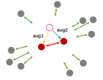
(a) Instance-level

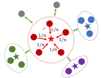
(b) Cluster-level

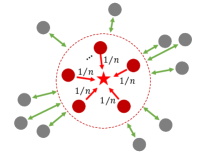
(c) HCL

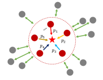
(d) MGCE-HCL

Figure 1: Illustration for different contrastive learning paradigms. Red arrows in a), b) and c): pulling together; Green arrows: pushing away. (a) For instance-level paradigm, two augmented samples (red points) of original input (red circle) are pulled together and push all others away. (b) For cluster-level paradigm, positive samples (red points) are pushed to the cluster center (red star), and different clusters are mutually exclusive. (c) In our HCL, different from (a) and (b), we consider all negative samples (grey points) individually as individual class. (d) In MGCE-HCL, we further use the priority to weight the similarity between positive samples.

In cluster-level contrastive learning, cluster information (i.e., pseudo labels), is generated by a clustering algorithm, and the similarity of the feature of the input image and the cluster centers (i.e., the mean vector of each cluster) is used to build an InfoNCE-like loss as follows:

$$\mathcal{L}_{con}=-\frac{1}{|\mathcal{B}|}\sum_{i=1}^{|\mathcal{B}|}{\log\frac{\exp(\left\langle\ \bm{f}_{x_{i}},\bm{\mu}_{+}\right\rangle/\tau)}{\sum_{j=1}^{C}\exp(\left\langle\ \bm{f}_{x_{i}},\bm{\mu}_{j}\right\rangle/\tau))}},$$ (1)

where $\tau>0$ is a temperature constant, $\mathcal{B}$ denotes a mini-batch of samples, $|\mathcal{B}|$ denotes the number of the samples in $\mathcal{B}$, $C$ denotes the number of clusters, $\bm{f}_{x_{i}}$ is the feature representation of an input $\bm{x}_{i}$, and $\bm{f}_{M_{i}}$ denotes the feature from memory bank with index $i$, in which $\bm{f}_{x_{i}}$ and $\bm{f}_{M_{i}}$ are defined as

$$\bm{f}_{M_{i}}\leftarrow\gamma\bm{f}_{x_{i}}+(1-\gamma)\bm{f}_{M_{i}},$$ (2)

$$\bm{f}_{M_{i}}\leftarrow\frac{\bm{f}_{M_{i}}}{\left\|\bm{f}_{M_{i}}\right\|_{2}},$$ (3)

and $\bm{\mu}_{+}$ denotes the mean vector of the samples (i.e., positive sample) of the cluster to which $\bm{x}_{i}$ belongs, and $\bm{\mu}_{j}$ denotes the mean vector of the samples in the $j$-th cluster. The reason to use the memory bank $\mathcal{M}$ is that the features from memory bank is relative static and thus are not only more suitable to perform clustering algorithm for generating pseudo labels but also used as a reference for contrastive learning. Nevertheless, the dynamic features $\bm{f}_{x_{i}}$ extracted from the backbone are more appropriate for dynamic inputs due to containing more information from the random sample augmentation.

For clarity, we illustrate the mechanisms in instance-level contrastive learning and cluster-level contrastive learning in Fig. 1 (a) and (b). Note that both instance-level contrastive learning and cluster-level contrastive learning have shortcomings. Instance-level contrastive learning digs self-supervision information individually for each sample, ignoring the structure or correlation information among samples (e.g., cluster information), which is of vital importance especially for positive samples. For cluster-level contrastive learning, while it has been applied to the task such as person ReID, it introduces too much structural information for negative samples, which is usually useless in practice.

3.2 Hybrid Contrastive Learning (HCL) based Unsupervised Person ReID

To tackle the deficiencies mentioned above, we present a modified contrastive learning paradigm, which is a hybrid between the instance-level paradigm and the cluster-level paradigm, and thus is termed Hybrid Contrastive Learning (HCL).

The HCL framework consists of three components: a) an encoder module for learning convolution feature, b) a memory bank to store the updated features of the whole dataset, and c) a clustering module for generating pseudo labels. We adopt ResNet-50 [11] without the full-connection (FC) layer as the encoder module and denote the memory bank as $\mathcal{M}=\left\{\bm{f}_{M_{i}}\right\}_{i=1}^{N}$ which is used to store all the features during the training, where $N$ denotes the total number of samples in the dataset. The memory bank is initialized by the normalized features extracted from ResNet-50, which is pre-trained with ImageNet.

In training phase, we feed a batch of images, denoted as $\mathcal{B}$, into the backbone and then update the memory bank $\mathcal{M}$ with the new features via Eq. (2), where $\bm{f}_{M_{i}}$ denotes the feature representation of the sample $\bm{x}_{i}$ in the memory $\mathcal{M}$ and $\bm{f}_{\bm{x}_{i}}$ is the convolution feature of the input $\bm{x}_{i}$ extracted by the backbone. We adopt the DBSCAN algorithm [3] with a fixed parameter $d$ to generate the pseudo labels. While the pseudo labels are noisy, there are still rich supervision information for contrastive learning.

In this paper, to remedy the deficiencies in instance-level and cluster-level contrastive learning, we propose a hybrid contrastive loss as follows:

$$\!\!\!\mathcal{L}_{HCL}=-\frac{1}{|\mathcal{B}|}\!\!\sum_{i=1}^{|\mathcal{B}|}{\log\frac{\exp(\left\langle\ \bm{f}_{x_{i}},\bm{\mu}_{+}\right\rangle/\tau)}{\exp(\left\langle\bm{f}_{x_{i}},\bm{\mu}_{+}\right\rangle/\tau)+\sum_{j\notin\bm{\omega}_{+}}{\exp(\left\langle\ \bm{f}_{x_{i}},\bm{f}_{M_{j}}\right\rangle/\tau)}}},$$ (4)

where $\bm{\mu}_{+}$ denotes the mean of the positive samples of $\bm{f}_{x_{i}}$, $|\mathcal{B}|$ denotes the batch size, and $j\notin\bm{\omega}_{+}$ denotes to the index set of samples that do not belong to the current cluster $\bm{\omega}_{+}$ which corresponds to $\bm{\mu}_{+}$. For clarity, we illustrate the hybrid contrastive paradigm in Fig. 1 (c).

Remark 1. In the modified contrastive loss Eq. (4), we reserve the cluster information for positive samples (i.e., which corresponds to positive cluster) which is able to pull the similar samples together, and at the same time, we treat all the remaining samples—other than the positive samples—as negative samples, rather than using the mean vectors of other (negative) clusters. The reasons are two-folds: a) since that the primal goal of the contrastive learning is to pull positive samples together and push all negative samples away, it is not needed to care the cluster information of the negative samples; and b) more negative samples are used, more contrasting information can be provided and thus help to avoid obtaining a trivial solution [9, 16].

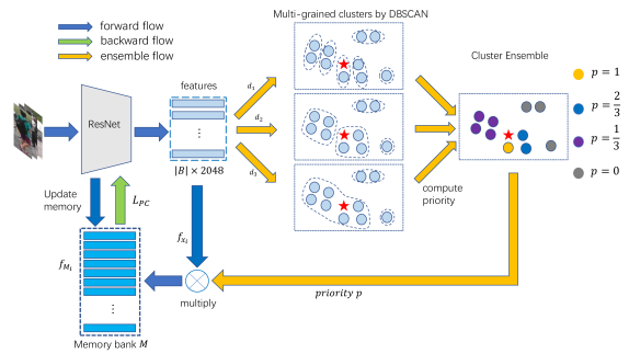
Figure 2: Architecture of MGCE-HCL. The figure shows the case that three clustering results are assembled. Each batch of images are fed into ResNet50 to obtain the features, and then DBSCAN with parameter $d$ is used to perform clustering with the features in the memory bank. After that, we compute priority matrix with multiple granularity cluster results. In Cluster Ensemble (CE) module, different colors of points denote different value of priority and the red star denotes the convolution features of the current sample. To compute $\mathcal{L}_{PC}$, we compute the cosine similarity between the input features and the features in memory bank with priority-weighting mechanism.

4 Hybrid Contrastive Learning with Multi-Granularity Cluster Ensemble (MGCE-HCL)

This section presents a Hybrid Contrastive Learning framework with Multi-Granularity Clustering Ensemble (MGCE-HCL) for unsupervised person ReID.

Compared to HCL, the key differences of MGCE-HCL are two-folds: a) rather than performing DBSCAN with a single neighborhood parameter $d$ to yield a clustering result, we perform DBSCAN multiple times with parameter $d$ sampled in a range to generate a multi-granularity clustering results and encode the obtained clustering results into priority weights; and b) we introduce the priority weights into the hybrid contrastive loss, which automatically exploits the confidence of the positive sample pairs.

Multi-Granularity Clustering Ensemble (MGCE). To remedy the sensitivity to the hyper-parameter in DBSCAN, we perform DBSCAN $T$ times, each time using a different neighborhood parameter $d^{(\ell)}$, in which $\{{d^{(\ell)}}\}_{\ell=1}^{T}$ are sampled from a range with an interval $\delta$. Let $\bm{c}^{(\ell)}$ be the obtained cluster index of the $\ell$-th clustering with parameter $d^{(\ell)}$, where $\ell=1,\cdots,T$. Accordingly we define an affinity matrix $A^{(\ell)}$, which is calculated as follows:

$$\begin{split}&A_{i,j}^{(\ell)}=\left\{\begin{array}[]{ll}1,~{}~{}~{}{c}_{i}^{(\ell)}={c}_{j}^{(\ell)}\\ 0,~{}~{}~{}{c}_{i}^{(\ell)}\neq{c}_{j}^{(\ell)}.\end{array}\right.\end{split}$$ (5)

Note that $A_{i,j}^{(\ell)}$ is obtained with the neighborhood parameter taking the value $d^{(\ell)}$ and thus we view $A_{i,j}^{(\ell)}$ as the affinity under a specific granularity indexed with $d^{(\ell)}$. By taking an average over the $T$ results, we have a priority weight as follows:

$$p_{i,j}=\frac{1}{T}\sum_{\ell=1}^{T}A_{i,j}^{(\ell)},$$ (6)

where $0\leq p_{i,j}\leq 1$ approximately quantifies the confidence of two samples being grouped into the same cluster.

Remark 2. From a geometrical perspective, the priority is to describe the neighboring relationship between any two samples. This is because that if two samples lie close enough—they are more likely to be grouped into the same small cluster and thus are certainly to be grouped into larger cluster, resulting a higher priority value according to Eq. (6). From the probabilistic perspective, the priority also measures the confidence that the two samples are in the same cluster. Briefly, the higher the priority is, the two samples are more likely to be closer and the sample pairs are more credible to be positive samples. On contrary, when the priority of two samples is 0, it is reasonable to consider them as negative samples.

Priority-Weighted Hybrid Contrastive Loss. Given the priority weights, we propose a priority-weighted hybrid contrastive loss as follows:

$$\begin{split}\mathcal{L}_{PC}=-\frac{1}{|\mathcal{B}|}\sum_{i=1}^{|\mathcal{B}|}{\log\frac{s_{i}^{+}}{s_{i}^{+}+s_{i}^{-}}},\end{split}$$ (7)

in which $s_{i}^{+}$ and $s_{i}^{-}$ are defined as the exponential similarity between the input and the positive samples and between the input and the negative samples, respectively, i.e.,

$$s_{i}^{+}=\exp(\frac{\sum_{j=1}^{N}{p_{i,j}\left\langle\bm{f}_{x_{i}},\bm{f}_{M_{j}}\right\rangle/\tau}}{\sum_{j=1}^{N}{p_{i,j}}}),$$ (8)

$$s_{i}^{-}=\sum_{j=1}^{N}{\mathbb{I}(p_{i,j}=0)\exp(\left\langle\bm{f}_{x_{i}},\bm{f}_{M_{j}}\right\rangle/\tau)},$$ (9)

where $\mathbb{I}(\cdot)$ is an indicator function, $\mathbb{I}(p_{i,j}=0)$ outputs $1$ if $p_{i,j}=0$, and $\left\langle\cdot,\cdot\right\rangle$ denotes the inner product. Note that $s_{i}^{+}$ is computed by the inner product between the feature of the input image and the features from the memory bank $\mathcal{M}$ and are weighted by the nonzero priority; whereas $s_{i}^{-}$ is computed by the samples whose priority being $0$ which are considered as negative samples and each negative sample pair is treated individually ignoring their cluster information.

For clarity, we provide the flowchart of the MGCE-HCL framework in Fig. 2. The input image is shown as the red star in the cluster ensemble module. After obtaining the confidence of all sample pairs, we weight each sample pair with the accumulated priority to train the whole model.

Remark 3. Note that priority-weighted similarity defined in Eq. (8) can bring more information for positive samples pairs because, the priority is able to describe the density of samples. For the computation of positive scores, we use priority to weight the positive samples of different distance but the cluster-level contrastive loss and HCL only compute the similarity between the input and the mean vector of all positive samples, which is equivalent to give each positive sample the same weight. For the negative samples, both MGCE-HCL and HCL consider each negative sample individually without using cluster information. For clarity, the difference between HCL and MGCE-HCL is illustrated in Fig. 1 (d).

5 Experiments

5.1 Datasets and Evaluation Metrics

Datasets. We evaluate our method with two benchmark datasets: Market-1501[28] and DukeMTMC-reID[17]. Market1501 has total 12,936 images of 751 identities in the training set, and in total 19,732 images of 750 identities; whereas DukeMTMC-reID has total 16,522 images of 702 identities in the training set, and in total 19,989 images of 702 identities.

Evaluation Metrics. We use two popular metrics for person ReID, including Cumulative Match Characteristic (CMC) and mean Average precision (mAP). For CMC, we only use top-1 to evaluate the performance.

5.2 Implementation Details

Our MGCE-HCL adopts ImageNet to pretrain ResNet50 as the backbone. Each input is resized to $256\times 128$, and is transformed by horizontal flip and random erasing [29], whose probabilities are all set to 0.5. The range of the parameter $d$ in MGCE are set as $[0.4,0.6]$ with interval $\delta=0.05$. The parameter $\tau$ in the loss $\mathcal{L}_{PC}$ in Eq. (7) is set to 0.05 and the momentum parameter $\gamma$ in Eq. (2) is set to 0.2. During the training, following the protocol in the prior work, we select 16 pseudo identities and 4 samples per identity as each mini-batch, and train totally 50 epochs. In experiments, we utilize the Adam optimizer [12] to optimize the network with a weight decay rate $5\times 10^{-4}$.

5.3 Ablation Study

To validate the effectiveness of each component in our proposals, we conduct a set of ablation experiments.

HCL vs. Cluster-level and Instance-level based Methods. In HCL, we use the negative samples without any clustering structural information. To validate the effectiveness of our approach, we compare our HCL approach with the cluster-level contrastive learning method, which is marked as “clusterNCE”, and the instance-level contrastive learning method which is represented by MoCo [10]. We conduct a set of experiments with the commonly used best-performing parameter $d$ in DBSCAN as in prior works [7, 6, 27, 20]. Experimental results are reported in Table 1. We can read from the table that our HCL outperforms the instance-level and cluster-level contrastive learning methods in all cases. This is because that our hybrid contrastive learning paradigm can well grasp the useful information and effectively eliminate the impact of negative samples compared to MoCo and clusterNCE.

Table 1: HCL vs. clusterNCE and MoCo. The results of MoCo are cited from [7].

Method	Market-1501		DukeMTMC-reID
	mAP	top-1	mAP	top-1
MoCo[10]	6.1	12.8	5.6	10.7
clusterNCE ($d=0.4$)	69.2	86.8	59.0	76.2
HCL ($d=0.4$)	74.6	89.4	61.1	77.2
clusterNCE ($d=0.5$)	73.9	87.9	63.6	79.2
HCL ($d=0.5$)	79.4	91.7	66.2	81.3
clusterNCE ($d=0.6$)	68.9	85.5	62.5	78.6
HCL ($d=0.6$)	77.2	90.1	67.4	81.8

Table 2: Comparison of MGCE-HCL and HCL with different $d$

Method	Market-1501		DukeMTMC-reID
	mAP	top-1	mAP	top-1
HCL ($d=0.40$)	74.6	89.4	61.1	77.2
HCL ($d=0.45$)	77.4	90.9	63.3	78.2
HCL ($d=0.50$)	79.4	91.7	66.2	81.3
HCL ($d=0.55$)	79.0	91.2	67.0	82.5
HCL ($d=0.60$)	77.2	90.1	67.4	81.8
MGCE-HCL ($d\in[0.4,0.6]$)	79.6	92.1	67.5	82.5

MGCE-HCL vs. HCL. In HCL, we perform DBSCAN with a fixed neighborhood radius parameter $d$ to obtain a specific clustering result and thus the pseudo labels; whereas in MGCE, we perform DBSCAN for multiple times, each time with a different parameter $d$, to obtain multiple clustering results. In previous DBSCAN based methods, it has been reported that the best-performing results are obtained usually when $d$ is taking the value from 0.4 to 0.6. This means that performing clustering with $d$ in such an interval will gain the most useful clustering information. To demonstrate the effectiveness of our clustering ensemble strategy, we compare our MGCE-HCL with HCL, in which both of them use $d$ taking from $0.4$ to $0.6$ in an interval of $0.05$. The experimental results are shown in Table  2. We can observe that HCL performs best when $d$ is set to 0.5 for Market-1501 and 0.55 or 0.6 for DukeMTMC; whereas MGCE-HCL outperforms all the cases of HCL on both Market-1501 and DukeMTMC-reID.

Table 3: Evaluation on MGCE-HCL with different parameter ranges.

Ensemble Range	Market-1501		DukeMTMC-reID
	mAP	top-1	mAP	top-1
0.1-0.3	39.3	63.3	48.8	67.6
0.2-0.3	49.5	74.0	51.8	71.1
0.1-0.4	65.6	84.7	58.9	75.9
0.2-0.4	68.2	86.8	58.4	75.5
0.3-0.4	73.3	89.1	60.1	77.0
0.1-0.5	75.8	90.3	63.4	79.7
0.2-0.5	77.5	91.3	63.5	79.2
0.3-0.5	78.2	91.1	64.6	80.1
0.4-0.5	79.3	91.4	64.9	80.7
0.1-0.6	79.0	91.5	67.0	81.7
0.2-0.6	79.1	91.0	67.2	81.9
0.3-0.6	79.4	91.8	66.8	81.3
0.4-0.6	79.6	92.1	67.5	82.5
0.5-0.6	78.1	91.3	67.3	81.5
0.3-0.7	17.7	35.4	7.8	15.1
0.4-0.7	50.0	74.0	46.8	64.7

Table 4: Evaluation on MGCE-HCL with different interval $\delta$.

Interval $\delta$	Market-1501		DukeMTMC-reID
	mAP	top-1	mAP	top-1
0.05	79.6	92.1	67.5	82.5
0.02	78.8	91.2	67.0	81.8
0.01	79.5	91.7	67.2	81.5

Table 5: Evaluation on MGCE-HCL with Different $\gamma$.

$\gamma$	Market-1501		DukeMTMC-reID
	mAP	top-1	mAP	top-1
0.1	78.8	91.1	67.1	81.6
0.2	79.6	92.1	67.5	82.5
0.3	79.6	92.0	67.0	81.4
0.4	79.3	91.7	66.0	80.5
0.5	79.0	91.4	64.3	79.9

Table 6: Comparison to SOTA methods on Market-1501 and DukeMTMC.

Type	Method	Reference	Market-1501		DukeMTMC-reID
			mAP	top-1	mAP	top-1
UDA	PTGAN [21]	CVPR’18	15.7	38.6	13.5	27.4
	SPGAN [2]	CVPR’18	26.7	58.1	26.4	46.9
	HHL[30]	ECCV’18	31.4	62.2	27.2	46.9
	ECN[31]	CVPR’19	43.0	75.1	40.4	63.3
	SSG [5]	ICCV’19	58.3	80.0	53.4	73.0
	MMCL[18]	CVPR’20	60.4	84.4	51.4	72.4
	ECN++[32]	TPAMI’20	63.8	84.1	54.4	74.0
	AD-cluster[26]	CVPR’20	68.3	86.7	54.1	72.6
	MMT[6]	ICLR’20	73.8	89.5	62.3	76.3
	SpCL[7]	NeuIPS’20	76.7	90.3	68.8	82.9
USL	LOMO[13]	CVPR’15	8.0	27.2	4.8	12.3
	BoW[28]	ICCV’15	14.8	35.8	8.5	17.1
	PUL[4]	TOMM’18	22.8	51.5	22.3	41.1
	CAMEL[23]	ICCV’17	26.3	54.4	19.8	40.2
	BUC[14]	AAAI’19	30.6	61.0	21.9	40.2
	SSL[15]	CVPR’20	37.8	71.7	28.6	52.5
	HCT[25]	CVPR’20	56.4	80.0	50.1	69.6
	SpCL[7]	NeurIPS’20	72.6	87.7	65.3	81.2
	CAP[20]	AAAI’21	79.2	91.4	67.3	81.1
	HCL	This paper	77.2	90.1	67.4	81.8
	MGCE-HCL	This paper	79.6	92.1	67.5	82.5

Evaluation on Parameter Range for MGCE-HCL. To explore the proper range to sample the parameter $d$, we conduct experiments with $d$ sampled in different ranges and show the results in Table 3. Since that the parameter $d$ is used to determine the neighborhood, it is not reasonable to set it too large and the same for the upper bound of the parameter range in MGCE. According to the experience, when $d$ is set in the range of $[0.4,0.6]$, the cluster results might combine positive samples and moderate noises which contain rich and reliable clustering information. To make full use of such clustering information in the range of $[0.4,0.6]$, we set the upper bound of the parameter range as $0.5,0.6,0.7$, respectively, and increase the lower bound of the range from $0.1$ and using an interval $\delta=0.05$ for fair comparison. We also add the experiments with the upper bound of 0.4 to validate the robustness of our MGCE-HCL. Experiments are shown in Table 3. We can read that when the upper bound is $0.6$, MGCE-HCL yields better performance. Especially when the lower bound is set as $0.4$, MGCE-HCL achieves the best performance. This result suggests that the range of $[0.4,0.6]$ for the parameter $d$ to perform DBSCAN contains the richest clustering information and it is consistent with the common practice for setting the parameter $d$ in prior works [7, 6, 27, 20]. Moreover, we find that decreasing the lower bound may cause slight drop on the performance. The reason is that when the upper bound is fixed, decreasing the lower bound will decrease the priority of samples from clusters of larger size, which may contain more useful information. It is worth to note that MGCE-HCL is insensitive to the lower bound of ensemble range and not that sensitive to the upper bound of the range when the upper bound is not over-large. This hints that we can obtain reasonably good performance with a relatively larger range for clustering ensemble and an appropriate upper bound even if we do not know the exact best parameter $d$. However, as shown in Table 3, the results might sharply drop when we set the upper bound up to 0.7. It is because that the clustering results will be too noisy when using an over-large parameter $d$.

Evaluation on $\delta$ in Cluster Ensemble. To evaluate the effect of the interval in the ensemble range, we fix the parameter range to pick $d$ as $[0.4,0.6]$ and change the sampling interval $\delta$ to $\{0.05,0.02,0.01\}$, individually. Experimental results are shown in Table 4. Using a smaller $\delta$ leads to a larger $T$, i.e., the times of running DBSCAN. The results show that MGCE-HCL is also insensitive to the interval $\delta$.

Evaluation on momentum factor $\gamma$. As shown in Eq. 2, parameter $\gamma$ is the momentum factor to update memory bank. In our method, memory bank is used to store relatively static features (i.e.smoothed features), rather than using the features directly extracted from the output of the backbone. Therefore, the momentum factor $\gamma$ should not be too large. To evaluate the effect of using different parameter $\gamma$, we conduct a set of experiments to compare the performance with different $\gamma$ in Table 5. The results show that $\gamma=0.2$ achieves the best performance and the performance gradually drops when $\gamma$ is larger than 0.2.

5.4 Comparison to State-of-the-art Methods

Finally, we compare the performance of our proposed MGCE-HCL method to the state-of-the-art methods on Market-1501 and DukeMTMC-reID. The experimental results are shown in Table  6.

Compared to USL-based methods. We compare the most unsupervised works recent years, including BoW [28], LOMO [13], PUL [4], CAMEL [23], BUC [14], SSL [15], HCT [25], SpCL [7] and CAP [20]. In the USL-based methods, only the unlabeled data is used. In most recent works, e.g., BUC, HCT, SpCL and CAP, they are based on a clustering method (e.g., $k$-means, DBSCAN, or hierarchical clustering) to yield the pseudo labels. Among them, SpCL and CAP also use cluster-based contrastive learning method. SpCL learns with a self-paced strategy and CAP introduces the camera information to boost training. Compared to CAP, our HCL obtains the comparable results on Market-1501 and obtains 0.7% top-1 and 0.1% mAP performance gain on DukeMTMC-reID, and our MGCE-HCL obtains 0.7% top-1 and 0.4% mAP performance gain on Market-1501, and obtains 1.4% top-1 gain and 0.2% mAP gain on DukeMTMC-reID, respectively.

Compared to UDA-based methods. We also list the results for UDA based methods at the upper part in Table 6. The UDA-based methods exploit the information from source domain to improve the performance of unlabeled target domain. In the UDA part, the column of Market-1501 shows the results where model is transferred from DukeMTMC-reID to Market-1501, and vice versa for the column of DukeMTMC-reID. Note that our methods without any label annotation can outperform SpCL on Market-1501 and are on par with SpCL on DukeMTMC-reID.

6 Conclusions

We have proposed a hybrid contrastive learning (HCL) paradigm for unsupervised person ReID, in which the cluster structure of positive samples are reserved but the clusters of the negative samples are ignored. Moreover, we have presented a multi-granularity cluster ensemble (MGCE) approach to weight the positive samples in different granularity with a priority, and developed a priority-weighted hybrid contrastive loss for training, by which the noises especially from larger granularity clusters can be reduced to some extent. We conducted extensive experiments on two benchmark datasets and the results shown that our HCL paradigm notably outperforms the instance-level contrastive learning paradigm and cluster-level contrastive learning paradigm, and our MGCE-HCL approach achieves the better performance compared to state-of-the-art methods.

References

- [1] Chen, T., Kornblith, S., Norouzi, M., Hinton, G.: A simple framework for contrastive learning of visual representations. In: International conference on machine learning. pp. 1597–1607. PMLR (2020)
- [2] Deng, W., Zheng, L., Ye, Q., Kang, G., Yang, Y., Jiao, J.: Image-image domain adaptation with preserved self-similarity and domain-dissimilarity for person re-identification. In: IEEE Conference on Computer Vision and Pattern Recognition. pp. 994–1003 (2018)
- [3] Ester, M., Kriegel, H.P., Sander, J., Xu, X.: A density-based algorithm for discovering clusters in large spatial databases with noise. In: Proceedings of the Second International Conference on Knowledge Discovery and Data Mining. p. 226–231 (1996)
- [4] Fan, H., Zheng, L., Yan, C., Yang, Y.: Unsupervised person re-identification: Clustering and fine-tuning. ACM Transactions on Multimedia Computing, Communications, and Applications 14(4), 83 (2018)
- [5] Fu, Y., Wei, Y., Wang, G., Zhou, Y., Shi, H., Huang, T.S.: Self-similarity grouping: A simple unsupervised cross domain adaptation approach for person re-identification. In: Proceedings of the IEEE/CVF International Conference on Computer Vision. pp. 6112–6121 (2019)
- [6] Ge, Y., Chen, D., Li, H.: Mutual mean-teaching: Pseudo label refinery for unsupervised domain adaptation on person re-identification. In: International Conference on Learning Representations (2020)
- [7] Ge, Y., Zhu, F., Chen, D., Zhao, R., Li, H.: Self-paced contrastive learning with hybrid memory for domain adaptive object re-id. In: Advances in Neural Information Processing Systems (2020)
- [8] Grill, J.B., Strub, F., Altché, F., Tallec, C., Richemond, P.H., Buchatskaya, E., Doersch, C., Pires, B.A., Guo, Z.D., Azar, M.G., et al.: Bootstrap your own latent: A new approach to self-supervised learning. arXiv preprint arXiv:2006.07733 (2020)
- [9] Gutmann, M., Hyvärinen, A.: Noise-contrastive estimation: A new estimation principle for unnormalized statistical models. Journal of Machine Learning Research 9, 297–304 (2010)
- [10] He, K., Fan, H., Wu, Y., Xie, S., Girshick, R.: Momentum contrast for unsupervised visual representation learning. In: Proceedings of the IEEE/CVF Conference on Computer Vision and Pattern Recognition. pp. 9729–9738 (2020)
- [11] He, K., Zhang, X., Ren, S., Sun, J.: Deep residual learning for image recognition. In: Proceedings of the IEEE conference on computer vision and pattern recognition. pp. 770–778 (2016)
- [12] Kingma, D.P., Ba, J.: Adam: A method for stochastic optimization. arXiv preprint arXiv:1412.6980 (2014)
- [13] Liao, S., Hu, Y., Zhu, X., Li, S.Z.: Person re-identification by local maximal occurrence representation and metric learning. In: IEEE Conference on Computer Vision and Pattern Recognition. pp. 2197–2206 (2015)
- [14] Lin, Y., Dong, X., Zheng, L., Yan, Y., Yang, Y.: A bottom-up clustering approach to unsupervised person re-identification. In: The Association for the Advancement of Artificial Intelligence. vol. 33, pp. 8738–8745 (2019)
- [15] Lin, Y., Xie, L., Wu, Y., Yan, C., Tian, Q.: Unsupervised person re-identification via softened similarity learning. In: IEEE Conference on Computer Vision and Pattern Recognition (2020)
- [16] Oord, A.v.d., Li, Y., Vinyals, O.: Representation learning with contrastive predictive coding. arXiv preprint arXiv:1807.03748 (2018)
- [17] Ristani, E., Tomasi, C.: Features for multi-target multi-camera tracking and re-identification. In: Proceedings of the IEEE conference on computer vision and pattern recognition. pp. 6036–6046 (2018)
- [18] Wang, D., Zhang, S.: Unsupervised person re-identification via multi-label classification. In: Proceedings of the IEEE/CVF Conference on Computer Vision and Pattern Recognition. pp. 10981–10990 (2020)
- [19] Wang, G., Yuan, Y., Chen, X., Li, J., Zhou, X.: Learning discriminative features with multiple granularities for person re-identification. In: Proceedings of the 26th ACM international conference on Multimedia. pp. 274–282 (2018)
- [20] Wang, M., Lai, B., Huang, J., Gong, X., Hua, X.S.: Camera-aware proxies for unsupervised person re-identification. In: Proceedings of the AAAI Conference on Artificial Intelligence (AAAI) (2021)
- [21] Wei, L., Zhang, S., Gao, W., Tian, Q.: Person transfer gan to bridge domain gap for person re-identification. In: IEEE Conference on Computer Vision and Pattern Recognition. pp. 79–88 (2018)
- [22] Wu, Z., Xiong, Y., Yu, S.X., Lin, D.: Unsupervised feature learning via non-parametric instance discrimination. In: Proceedings of the IEEE Conference on Computer Vision and Pattern Recognition. pp. 3733–3742 (2018)
- [23] Yu, H.X., Wu, A., Zheng, W.S.: Cross-view asymmetric metric learning for unsupervised person re-identification. In: IEEE International Conference on Computer Vision. pp. 994–1002 (2017)
- [24] Yu, H.X., Zheng, W.S., Wu, A., Guo, X., Gong, S., Lai, J.H.: Unsupervised person re-identification by soft multilabel learning. In: Proceedings of the IEEE/CVF Conference on Computer Vision and Pattern Recognition. pp. 2148–2157 (2019)
- [25] Zeng, K., Ning, M., Wang, Y., Guo, Y.: Hierarchical clustering with hard-batch triplet loss for person re-identification. In: IEEE Conference on Computer Vision and Pattern Recognition. pp. 13657–13665 (2020)
- [26] Zhai, Y., Lu, S., Ye, Q., Shan, X., Chen, J., Ji, R., Tian, Y.: Ad-cluster: Augmented discriminative clustering for domain adaptive person re-identification. In: Proceedings of the IEEE/CVF Conference on Computer Vision and Pattern Recognition. pp. 9021–9030 (2020)
- [27] Zhai, Y., Ye, Q., Lu, S., Jia, M., Ji, R., Tian, Y.: Multiple expert brainstorming for domain adaptive person re-identification. In: Computer Vision–ECCV 2020: 16th European Conference, Glasgow, UK, August 23–28, 2020, Proceedings, Part VII 16. pp. 594–611. Springer (2020)
- [28] Zheng, L., Shen, L., Tian, L., Wang, S., Wang, J., Tian, Q.: Scalable person re-identification: A benchmark. In: IEEE International Conference on Computer Vision. pp. 1116–1124 (2015)
- [29] Zhong, Z., Zheng, L., Kang, G., Li, S., Yang, Y.: Random erasing data augmentation. In: Proceedings of the AAAI Conference on Artificial Intelligence. vol. 34, pp. 13001–13008 (2020)
- [30] Zhong, Z., Zheng, L., Li, S., Yang, Y.: Generalizing a person retrieval model hetero-and homogeneously. In: European Conference on Computer Vision. pp. 172–188 (2018)
- [31] Zhong, Z., Zheng, L., Luo, Z., Li, S., Yang, Y.: Invariance matters: Exemplar memory for domain adaptive person re-identification. In: Proceedings of the IEEE/CVF Conference on Computer Vision and Pattern Recognition. pp. 598–607 (2019)
- [32] Zhong, Z., Zheng, L., Luo, Z., Li, S., Yang, Y.: Invariance matters: Exemplar memory for domain adaptive person re-identification pp. 598–607 (2019)