Shuffle Augmentation of Features from Unlabeled Data for
Unsupervised Domain Adaptation

Abstract

Unsupervised Domain Adaptation (UDA), a branch of transfer learning where labels for target samples are unavailable, has been widely researched and developed in recent years with the help of adversarially trained models. Although existing UDA algorithms are able to guide neural networks to extract transferable and discriminative features, classifiers are merely trained under the supervision of labeled source data. Given the inevitable discrepancy between source and target domains, the classifiers can hardly be aware of the target classification boundaries. In this paper, Shuffle Augmentation of Features (SAF), a novel UDA framework, is proposed to address the problem by providing the classifier with supervisory signals from target feature representations. SAF learns from the target samples, adaptively distills class-aware target features, and implicitly guides the classifier to find comprehensive class borders. Demonstrated by extensive experiments, the SAF module can be integrated into any existing adversarial UDA models to achieve performance improvements.

1 Introduction

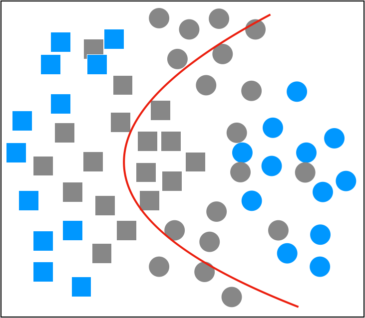
(a) source only

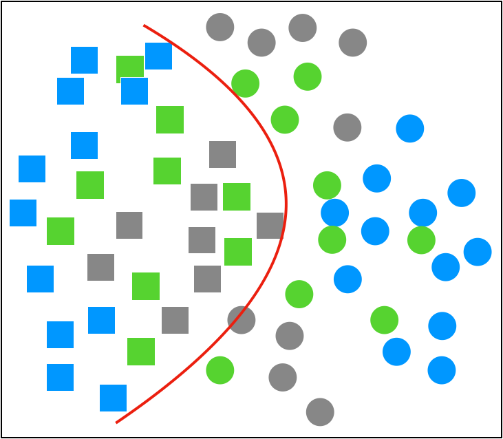
(b) SAF assisted

Figure 1: Illustration of the Shuffle Augmentation of Features (SAF) algorithm. Best viewed in color. Squares and circles indicate different classes. Blue shapes denote source samples, gray shapes denote unrecognized target samples, and green shapes are target samples selected by SAF. (LABEL:sub@fig:intuition_a) Result of a classifier merely trained with labeled source data. Although the classifier learns the optimal boundary for the source distribution, many target samples are still misclassified due to the domain discrepancy. (LABEL:sub@fig:intuition_b) Result of an SAF-improved classifier trained with both source and composite target features selected by SAF. Supervised by signals from both source and target domains, the classifier is able to learn a more comprehensive class boundary.

Transfer learning algorithms usually learn class-aware information from sufficiently labeled source data and finetune on the target domain to transfer semantic representations. The crux of transfer learning is the unavoidable discrepancy between the source and target domains, leading to the essential objective of eliminating such inconsistency. Unsupervised Domain Adaptation (UDA) is a subtopic in transfer learning where target labels are unavailable, meaning that learning domain discrepancy between datasets is even more challenging compared with its supervised counterpart.

The Domain Adaptation (DA) problem is formally introduced by [2], where the fundamental concepts of the discrete $\mathcal{H}\Delta\mathcal{H}$-divergence is established. Various methods, based on deep CNN backbones [23, 17, 18], are proposed to tackle UDA tasks by reducing domain discrepancy with explicit regularizations [51, 30, 48]. Inspired by Generative Adversarial Network (GAN) [13], Domain Adversarial Neural Network (DANN) [10] extracts domain-invariant features with adversarial approach and enlightens other adversarial UDA methods [50, 33, 43]. Margin Disparity Discrepancy (MDD) [61] further generalizes $\mathcal{H}\Delta\mathcal{H}$-divergence by providing a continuous discrepancy metric.

Although UDA training strategies have been proven to be capable of guiding CNNs to extract transferable as well as categorical features, only labeled source features are utilized for supervised training. In the situation shown in Figure 1(a), features of different classes are clearly separated, but the optimal classification boundary guided by source-only supervision misclassifies numerous target samples. Hence, expanding the supervised training datasets with target features is necessary for further improvements.

Noisy Label (NL) learning aims to train models under the presence of incorrect labels, which is similar to the scenario of target samples with noisy pseudo-labels in UDA. Despite major differences between the two settings, employing NL schemes to assist UDA training in selecting creditable target features is intuitively viable.

In this paper, we propose Shuffle Augmentation of Features (SAF), a novel UDA framework. Inspired by NL algorithms, SAF learns the distribution of target features, assigns credibility weight to each entry, and guides the classifier to learn comprehensive class boundaries, as illustrated in Figure 1(b). Moreover, SAF can be integrated into any existing adversarial UDA models, enhancing their performances. To summarize, our contributions are:

• We analyze the theoretic backgrounds of the UDA problem, reveal the shortcomings of UDA methods with source-only supervisions, and discover a novel solution on the basis of cutting-edge DA theories. Specifically, we tackle the issues by adding target samples to supervisory signals. To the best of our knowledge, we are the first to distill class-variant information from the entire target distributions.

• We assimilate ideas from NL methods, adapt procedural details to compensate major differences between NL and UDA settings, and integrate their essence into the design of UDA algorithms.

• We propose the Shuffle Augmentation of Features (SAF), which can be built upon any adversarial UDA methods. SAF learns from target domain distributions, assigns reliablility weights to pseudo-labeled samples, and augments the supervisory training signal.

• We demonstrate the superiority of SAF algorithm with extensive experiments on benchmark datasets, where the proposed method outperforms existing UDA models and presents the state-of-the-art performance.

2 Related Work

2.1 Unsupervised Domain Adaptation

The fundamental theory for the Domain Adaptation (DA) is formally introduced by [3, 2], where the $\mathcal{H}\Delta\mathcal{H}$-divergence along with the estimation formula for error boundary on the target distribution are formalized. Based on above theories, researchers combine deep CNN [40, 24] backbones [23, 17, 18] with statistical measurements [51, 30, 48, 32, 45, 29, 58] to shrink the gap between source and target features. Inspired by Generative Adversarial Network (GAN) [13], [10, 11] proposes the Domain Adversarial Neural Network (DANN), which is the first method employing an adversary player to implicitly align domain features. The adversarial design of DANN further inspires numerous algorithms [50, 33, 42, 35, 43, 31, 26].

Nevertheless, [5] reveals that the discriminability of the features extracted by DANN actually decreases at the same time. [61] ascribes the phenomenon to the limitations of the $\mathcal{H}\Delta\mathcal{H}$-divergence and proposes the Margin Disparity Discrepancy (MDD), an alternative inconsistency metric generalizable to multi-way classifiers, to estimate the $\mathcal{H}\Delta\mathcal{H}$-divergence.

Moreover, clustering-based methods [8, 20] assign virtual labels to target data and enforce the network to follow the cluster assumption [14]. GAN-based methods [44, 19, 27] augment data by directly employing GANs, while mixup-based methods [34, 56, 64] combine existing samples with the mixup [59] technique.

2.2 Noisy Label Learning

The Noisy Label (NL) learning aims to train models from massive but inaccurately labeled data in real-world scenarios, as clean datasets are usually expensive to obtain. Traditional NL algorithms address the issue by using statistical clustering techniques (e.g. bagging, boosting, k-nearest neighbor, etc.) to determine the reliablility of each label [47, 15]. With the help of deep CNNs, the following approaches are proposed to tackle the noisy data: assigning weights to samples w.r.t. their reliablility [60, 54, 38]; selection or creation of clean samples [25, 46]; or dynamically renewing labels for mislabeled data [16, 63].

3 Preliminaries

Given an input space $\mathcal{X}$ and a label space $\mathcal{Y}$, a domain [2] is defined as a pair $\langle\mathcal{D},f\rangle$, where $\mathcal{D}$ is a distribution on $\mathcal{X}$, and $f:\mathcal{X}\rightarrow\mathcal{Y}$ is a labeling function. In Unsupervised Domain Adaptation (UDA), there are two datasets: the labeled source dataset ($\mathcal{S}$, $\mathcal{Y}_{S}$), and the unlabeled target dataset $(\mathcal{T},\varnothing)$, drawn from different domains $\langle\mathcal{D}_{S},f_{S}\rangle$, $\langle\mathcal{D}_{T},f_{T}\rangle$, respectively. Due to the discrepancy between two domains, techniques capable of mining underlying statistic patterns from feature distributions are required.

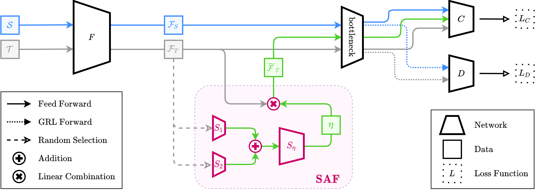
Figure 2: The SAF framework, best viewed in color. Built upon an adversarial UDA model consisting of a feature extractor $F$, a classifier $C$, and an adversarial module $D$, SAF further adds an SAF-mixup module and a bottleneck layer $B$. SAF randomly draws pairs of target features and adaptively generates mixup weights based on target distributions. The combined target features $\widetilde{\mathcal{F}}_{T}$ and corresponding pseudo-labels are used for augmentation of supervisory signals, enabling the model to discover better classification boundaries for target samples.

Let $\mathscr{C}$ be the hypothesis space of classifiers that map from the input space $\mathcal{X}$ to $[0,1]^{|\mathcal{Y}|}$. For an arbitrary $C\in\mathscr{C}$, $x\in\mathcal{X}$, and $y\in\mathcal{Y}$, denote $C_{y}(x)$ as the predicted probability for $x$ belonging to the class $y$, and denote $\hat{C}(x)$ as the predicted label for $x$. Margin Disparity Discrepancy (MDD) [61] is a continuous metric for divergence between two domains, which can be applied to design adversarial objectives beyond binary classifiers. Fixing the threshold $\varrho$, the empirical discrepancy $\hat{d}_{C,\mathscr{C}}^{(\varrho)}$ for a classifier $C$ on the hypothesis space $\mathscr{C}$ w.r.t. datasets $\mathcal{S}$, $\mathcal{T}$ is defined as:

$$\hat{d}_{C,\mathscr{C}}^{(\varrho)}(\mathcal{S},\mathcal{T})\triangleq\\ 2\max_{C^{\prime}\in\mathscr{C}}\big{(}\hat{\Delta}_{\mathcal{S}}^{(\varrho)}(C,C^{\prime})-\hat{\Delta}_{\mathcal{T}}^{(\varrho)}(C,C^{\prime})\big{)},$$ (1)

where $\hat{\Delta}_{\mathcal{S}}^{(\varrho)},\hat{\Delta}_{\mathcal{T}}^{(\varrho)}$ are the empirical margin disparity on datasets $\mathcal{S},\mathcal{T}$, respectively (definitions can be found in the supplementary material).

With probability at least $1-3\delta$ $(\delta>0)$, the risk for a classifier $C$ on the target domain $(\mathcal{D}_{T},f_{T})$ satisfies the following inequality:

$$\begin{split}\epsilon_{\mathcal{D}_{T}}(C)\leq\hat{\epsilon}_{\mathcal{S}}^{(\varrho)}(C)&+\hat{d}_{C,\mathscr{C}}^{(\varrho)}(\mathcal{S},\mathcal{T})+\lambda_{(\varrho,\mathscr{C},\mathcal{D}_{S},\mathcal{D}_{T})}\\ &+2\sqrt{\frac{\log\frac{2}{\delta}}{2|\mathcal{S}|}}+\sqrt{\frac{\log\frac{2}{\delta}}{2|\mathcal{T}|}}\\ &+K\Big{(}|\mathcal{Y}|,\frac{1}{\varrho},\frac{1}{\sqrt{|\mathcal{S}|}},\frac{1}{\sqrt{|\mathcal{T}|}}\Big{)},\end{split}$$ (2)

where $\hat{\epsilon}_{\mathcal{S}}^{(\varrho)}(C)$ is the empirical source risk, $\lambda$ is a constant, and $K$ is a term positively related to the number of classes $|\mathcal{Y}|$ and negatively related to the threshold $\varrho$ and the sizes of both source and target datasets.

However, following the definitions above, the concept of the hypothesis class $\mathscr{C}$ is questionable and not self-contained. For a fixed classifier structure, the hypothesis class $\mathscr{C}$ is invariable, but shrinking the discrepancy $\hat{d}_{C,\mathscr{C}}^{(\varrho)}(\mathcal{S},\mathcal{T})$ requires altering $\mathscr{C}$. In fact, another possible interpretation can be made to understand the theoretical backgrounds. Guided by various supervisory signals (e.g. loss criterions, regularizations), the process of optimizing CNNs can be regarded as squeezing the hypothesis class. Supervisions aim to lead CNNs to the optimized neighborhood $\mathscr{C}^{*}$ where the local discrepancy $\hat{d}_{C,\mathscr{C}^{*}}^{(\varrho)}(\mathcal{S},\mathcal{T})$ is the minimum across the universe:

$$\mathscr{C}^{*}\coloneqq\arg\min_{\mathscr{C}^{\prime}\subset\mathscr{C}}\big{[}\max_{C\in\mathscr{C}^{\prime}}\hat{d}_{C,\mathscr{C}^{\prime}}^{(\varrho)}(\mathcal{S},\mathcal{T})\big{]}.$$ (3)

In the rest of this paper, $\mathscr{C}$ denotes the hypothesis neighborhood of the current classifier $C$ guided by training strategies.

4 Shuffle Augmentation of Features

We propose the Shuffle Augmentation of Features (SAF) algorithm for the UDA problem.

4.1 Motivations

UDA is a special branch in the field of transfer learning, as there is no explicit clues about the target distribution and differences between domains $\mathcal{D}_{S}$ and $\mathcal{D}_{T}$. Existing state-of-the-art models [11, 61, 64] claim that they are capable of extracting features with decent transferability and discriminability from both source and target samples, but few of these algorithms utilize the target features for the training of the classifier $C$, yielding a suboptimal situation illustrated in Figure 1(a), where the optimal boundary for the source distribution misclassifies numerous target samples. Therefore, valuable target features shall be exploited to refine the classification boundaries, as shown in Figure 1(b).

The presence of labels is required for supervised training, so the estimated labels $\widehat{\mathcal{Y}}_{\mathcal{T}}$ are required. This introduces another intractable issue: since the pseudo-label estimation could not be completely accurate [20, 64], the network inevitably faces noisy labels. As the model needs to learn from correct labels and diminish the negative influences from incorrect labels, noise-robust algorithms are required to guarantee the convergence. Intuitively, NL learning [47, 15] is the desirable field where noise-robust algorithms have been widely studied and deeply developed.

4.2 Gaps Between NL and UDA

Although NL algorithms can effectively extract features with trustworthy labels from a noisy dataset, it is impractical to naively transfer NL methods to UDA due to three distinctions between the two settings:

1. In NL learning, all samples are from a unified domain distribution, but source and target distributions are inconsistent in the UDA setting.

2. Popular NL benchmark datasets [4, 57, 28] often contain massive amounts of samples, which are indeed favorable to pattern mining and clustering NL algorithms. By contrast, pervasive UDA benchmark datasets [41, 12, 53] offer only thousands or less samples per domain, where CNNs are more likely to overfit.

3. In the NL setting, the noise ratio are usually within the range of 8% to 38.5% [47]; but in UDA, source labels are always clean and there is no guaranteed maximal noise ratio for virtually labeled target samples.

The above differences between the two settings can potentially jeopardize the fitting of the NL training schemes, if transferred to the circumstance of UDA without reasonable adaptations.

4.3 Algorithm and Training Objectives

Tailored to the characteristics of the UDA setting, the SAF algorithm picks and incorporates the ideas of multiple NL methods [60, 16, 38]. The SAF framework is built upon an adversarial UDA backbone, where three main components (the feature generator $F$, the classifier $C$, and the adversarial module $D$) are presented. In addition, an SAF module and a bottleneck layer $B$ are added to the SAF algorithm. The SAF framework is shown in Figure 2.

Source Label Prediction Objective. Following the inequation 26 for the error boundary, the minimization of the source classification loss is necessary for decreasing the target risk. Since the bottleneck layer $B$ is added to regularize feature representations and takes part in prediction tasks, the training objective of source label prediction becomes:

$$(F^{*},B^{*},C^{*})\triangleq\arg\min_{F,B,C}L_{C}\big{(}[C\circ B\circ F](\mathcal{S}),\mathcal{Y_{S}}\big{)},$$ (4)

where $L_{C}$ is the classification criterion, usually the cross-entropy loss.

Adversarial Domain Adaptation Objective. The domain adversarial loss $L_{D}$ indicates the discrepancy between feature distributions $\mathcal{F}_{S}$ and $\mathcal{F}_{T}$. With the help of Gradient Reversal Layer (GRL) [10], $L_{D}$ guides the adversary module $D$ to regularize the extractor $F$ for finding features with better transferability.

In the proposed SAF framework, $(F,B)$ and $D$ play mini-max games to attain the optimum. In general, the domain adversarial objectives can be written as:

$$(F^{*},B^{*})\triangleq\arg\min_{F,B}\lambda_{D}L_{D}(F,B,D^{*},C^{*},\mathcal{S},\mathcal{T}),$$ (5)

$$D^{*}\triangleq\arg\max_{D}L_{D}(F^{*},B^{*},D,C^{*},\mathcal{S},\mathcal{T}).$$ (6)

where $\lambda_{D}$ is the GRL weight. The formula of $L_{D}$ completely depends on the design of the adversarial module $D$, which is determined by the UDA backbone selected.

For instance, if the MDD framework [61] were to be chosen as the backbone, $L_{D}$ would be:

$$L_{D}(F,B,D,C,\mathcal{S},\mathcal{T})\coloneqq\\ \mathbb{E}_{x\sim\mathcal{T}}\Big{[}\mathcal{L}_{\text{NLL}}\Big{(}1-\sigma\big{(}[D\circ B\circ F](x)\big{)}\Big{)}\Big{]}-\\ e^{\varrho}\cdot\mathbb{E}_{x\sim\mathcal{S}}\Big{[}-\mathcal{L}_{\text{NLL}}\Big{(}\sigma\big{(}[C\circ B\circ F](x)\big{)}\Big{)}\Big{]},$$ (7)

where $\mathcal{L}_{\text{NLL}}$ is the negative log likelihood loss, and $\sigma$ is the softmax function.

SAF-Supervision Objective. The SAF module (denoted as $M$) distills valuable target features via SAF-mixup, a novel mixup variant, to train the classifier $C$. As shown in Figure 2, the SAF module consists of two parallel bottlenecks $S_{1},S_{2}$, a weight estimator $S_{\eta}$, and two operation gates: a matrix addition gate $\bigoplus$ and a linear combination gate $\bigotimes$.

The motivation of using two independent SAF bottlenecks is straightforward: two NNs are able to extract diversified knowledge on the selection of valuable features, and they can learn from each other by backpropagation signals, which provides exceptional efficacy in training. In contrast, a single network not only lacks the diversity of a pair, but also feeds simplified information to $S_{\eta}$, impairing the effectiveness of the SAF module. The comparison is also investigated in ablation study (Table 5).

Module: bottleneck $B$, classifier $C$, SAF bottlenecks $S_{1}$, $S_{2}$, SAF weight estimator $S_{\eta}$

Input: the set of target features $\mathcal{F}_{T}$

Output: augmented features ($\widetilde{\mathcal{F}}_{T}$, $\widetilde{\mathcal{Y}}_{T}$)

1

2BEGIN:

3 $\widetilde{\mathcal{F}}_{T}\leftarrow\varnothing$;  $\widetilde{\mathcal{Y}}_{T}\leftarrow\varnothing$

4 while $\mathcal{F}_{T}\neq\varnothing$ do

5       $\phi_{1},\phi_{2}\leftarrow\operatorname{RandomDrawPair}(\mathcal{F}_{T})$

6       $\eta\leftarrow S_{\eta}\big{(}S_{1}(\phi_{1})+S_{2}(\phi_{2})\big{)}$

7       $\tilde{\phi}\leftarrow\eta\phi_{1}+(1-\eta)\phi_{2}$;

8       $\hat{y}_{1}\leftarrow C\circ B(\phi_{1});\>\hat{y}_{2}\leftarrow C\circ B(\phi_{2})$

9       $\tilde{y}\leftarrow\eta\hat{y}_{1}+(1-\eta)\hat{y}_{2}$

10       $\widetilde{\mathcal{F}}_{T}\leftarrow\widetilde{\mathcal{F}}_{T}\cup\{\tilde{\phi}\}$;  $\widetilde{\mathcal{Y}}_{T}\leftarrow\widetilde{\mathcal{Y}}_{T}\cup\{\tilde{y}\}$

11      

12 end while

END.

Algorithm 1 SAF-mixup

In SAF-mixup, target features extracted by $F$ are randomly selected as pairs, and parallelly fed into SAF bottlenecks. Then the sum of filtered features are forwarded into $S_{\eta}$, where the mixup coefficient $\eta$ is determined according to the relative confidence of the paired features. Afterwards, target features $\mathcal{F}_{T}$ and corresponding pseudo-labels $\widehat{\mathcal{Y}}_{T}$ are linearly combined with mixup coefficients to yield the augmentation dataset $(\widetilde{\mathcal{F}}_{T},\widetilde{\mathcal{Y}}_{T})$. As the augmented target features are forwarded into the bottleneck $B$ and the classifier $C$, the supervisory loss signals can be calculated and broadcasted to network structures via backpropagation. The SAF-supervision loss is calculated using the output logits and the corresponding composite labels $\widetilde{\mathcal{Y}}_{T}$:

$$L_{M}(\widetilde{\mathcal{F}}_{T},\widetilde{\mathcal{Y}}_{T})\coloneqq\mathcal{L}_{\text{CED}}\big{(}[C\circ B](\widetilde{\mathcal{F}}_{T}),\widetilde{\mathcal{Y}}_{T}\big{)},$$ (8)

where $\mathcal{L}_{\text{CED}}$ is the cross-entropy divergence (defined in the supplementary material).

Accordingly, the SAF-supervision objective can be described as the following:

$$(F^{*},M^{*},B^{*},C^{*})\triangleq\arg\min_{F,M,B,C}\lambda_{M}L_{M}(\widetilde{\mathcal{F}}_{T},\widetilde{\mathcal{Y}}_{T}),$$ (9)

where $\lambda_{M}$ is the SAF weight.

In SAF framework, $M$ is an adaptive Multi-Layer Perceptron (MLP) trained simultaneously with other prediction modules, as $M$ is adjusted to yield reliable mixup coefficients. Since $F,B,C$ are trained with comparatively ample data samples, beneficial mutations of $M$ will be positively amplified, while harmful gradients of $M$ that negatively affects the fitting can be amended and rectified.

The SAF module makes up the deficiencies of UDA models with source-only supervision. With the help of SAF, models are able to learn both source and target distributions and to perceive more accurate boundaries for target samples.

The Bottleneck Layer. As $C$ is only trained with source features, target feature fragments generated by SAF would be treated as noises and little meaningful information about the target distributions could be obtained. To address this issue, we propose the bottleneck $B$, which is able to reshape $\widetilde{\mathcal{F}}_{T}$ to match the subsequent classifier $C$, because $B$ learns from both source and target distributions. The necessity of the bottleneck in the SAF training scheme is also verified quantitatively in Section 5.3.

4.4 Theoretical Insight

We provide a theoretical justification of how the proposed SAF squeezes the error boundary according to the margin theories [61], and explains why SAF effectively seeks for novel weight-assigning strategy for noisy label learning. More details have been written in the Appendix. Let $C$ be the hypothesis we are interested in and denote $\mathscr{C}$ as its hypothesis neighborhood. Since $C$ digests feature representations $\mathcal{F}_{S}$ and $\mathcal{F}_{T}$, the error boundary in formula 26 can be rewritten as:

$$\begin{split}\epsilon_{\mathcal{F}_{T}}(h)\leq\epsilon_{\mathcal{F}_{S}}^{(\varrho)}(h)&+\hat{d}_{C,\mathscr{C}}^{(\varrho)}(\mathcal{F}_{S},\mathcal{F}_{T})+\lambda_{(\varrho,\mathscr{C},\mathcal{D}_{S},\mathcal{D}_{T})}\\ &+2\sqrt{\frac{\log\frac{2}{\delta}}{2|\mathcal{F}_{S}|}}+\sqrt{\frac{\log\frac{2}{\delta}}{2|\mathcal{F}_{T}|}}\\ &+K\Big{(}|\mathcal{Y}|,\frac{1}{\varrho},\frac{1}{\sqrt{|\mathcal{F}_{S}|}},\frac{1}{\sqrt{|\mathcal{F}_{T}|}}\Big{)}.\end{split}$$ (10)

As explained previously, the SAF algorithm generates augmented target features and expands the supervisory dataset, which is equivalent to enlarging the source sample space with $\widetilde{\mathcal{F}}_{T}$ and increasing the source sample size by $|\widetilde{\mathcal{F}}_{T}|$. Since the sum of specific terms in formula 10 decreases as we increase sample size of the source features $|\mathcal{F}_{S}|$, the following inequality holds:

$$2\sqrt{\frac{\log\frac{2}{\delta}}{2|\mathcal{F}_{S}\cup\widetilde{\mathcal{F}}_{T}|}}+K\Big{(}|\mathcal{Y}|,\frac{1}{\varrho},\frac{1}{\sqrt{|\mathcal{F}_{S}\cup\widetilde{\mathcal{F}}_{T}|}},\frac{1}{\sqrt{|\mathcal{F}_{T}|}}\Big{)}\\ <2\sqrt{\frac{\log\frac{2}{\delta}}{2|\mathcal{F}_{S}|}}+K\Big{(}|\mathcal{Y}|,\frac{1}{\varrho},\frac{1}{\sqrt{|\mathcal{F}_{S}|}},\frac{1}{\sqrt{|\mathcal{F}_{T}|}}\Big{)},$$ (11)

proving that SAF is capable of squeezing the error boundary on the basis of margin theories.

Moreover, Active Learning theories [6] and applications in deep CNNs [21, 9, 1] have proven that learning from data with uncertain labels dramatically improves the performance of deep CNNs. Using the conditional entropy $H\big{(}C(x)\big{)}=\sum_{y\in\mathcal{Y}}C_{y}(x)\log C_{y}(x)\>$as the uncertainty criterion, samples with ambiguous predictions shall be reused to reinforce the model fitting. On the one hand, reliable (or low-entropy) target samples, usually close to existing source clusters, intensify the biases from the source distribution instead of guiding the model to transfer semantic expressions. On the other hand, pseudo-labels for unreliable samples are more likely to be incorrect and noisy, which also degrade the model performance.

Therefore, the shuffle mixup among all target samples is utilized to address such dilemma. The diversity extracted from high-entropy samples is learnt by the network to fit on target distributions, while reliable samples offer trusty information to rectify influences of noisy gradients. The SAF module learns from the backpropagation signals to seek for the optimal weight-assigning strategy that balances between the biases brought by the low-entropy samples and the noises from high-entropy samples. The visualization in Figure 3 demonstrates the decent ability of SAF to cluster noisy target samples while simultaneously maintaining clear class boundaries.

Method	A $\to$ W	D $\to$ W	W $\to$ D	A $\to$ D	D $\to$ A	W $\to$ A	Avg
Source only	68.4$\pm$0.2	96.7$\pm$0.1	99.3$\pm$0.1	68.9$\pm$0.2	62.5$\pm$0.3	60.7$\pm$0.3	76.1
DAN [30]	80.5$\pm$0.4	97.1$\pm$0.2	99.6$\pm$0.1	78.6$\pm$0.2	63.6$\pm$0.3	62.8$\pm$0.2	80.4
DANN [10]	82.0$\pm$0.4	96.9$\pm$0.2	99.1$\pm$0.1	79.7$\pm$0.4	68.2$\pm$0.4	67.4$\pm$0.5	82.2
ADDA [50]	86.2$\pm$0.5	96.2$\pm$0.3	98.4$\pm$0.3	77.8$\pm$0.3	69.5$\pm$0.4	68.9$\pm$0.5	82.9
JAN [33]	86.0$\pm$0.4	96.7$\pm$0.3	99.7$\pm$0.1	85.1$\pm$0.4	69.2$\pm$0.3	70.7$\pm$0.5	84.6
MADA [35]	90.0$\pm$0.1	97.4$\pm$0.1	99.6$\pm$0.1	87.8$\pm$0.2	70.3$\pm$0.3	66.4$\pm$0.3	85.2
GTA [44]	89.5$\pm$0.5	97.9$\pm$0.3	99.8$\pm$0.4	87.7$\pm$0.5	72.8$\pm$0.3	71.4$\pm$0.4	86.5
MCD [43]	89.6$\pm$0.2	98.5$\pm$0.1	100.0$\pm$0.0	91.3$\pm$0.2	69.6$\pm$0.1	70.8$\pm$0.3	86.6
CDAN [31]	94.1$\pm$0.1	98.6$\pm$0.1	100.0$\pm$0.0	92.9$\pm$0.2	71.0$\pm$0.3	69.3$\pm$0.3	87.7
BSP [5]	93.3$\pm$0.2	98.2$\pm$0.2	100.0$\pm$0.0	93.0$\pm$0.2	73.6$\pm$0.3	72.6$\pm$0.3	88.5
CAT [8]	94.4$\pm$0.1	98.0$\pm$0.2	100.0$\pm$0.0	90.8$\pm$1.8	72.2$\pm$0.2	70.2$\pm$0.1	87.6
SymNets [62]	90.8$\pm$0.1	98.8$\pm$0.3	100.0$\pm$0.0	93.9$\pm$0.5	74.6$\pm$0.6	72.5$\pm$0.5	88.4
ImA [20]	90.3$\pm$0.2	98.7$\pm$0.1	99.8$\pm$0.0	92.1$\pm$0.5	75.3$\pm$0.2	74.9$\pm$0.3	88.8
CCC-GAN [27]	93.7$\pm$0.2	98.5$\pm$0.1	99.8$\pm$0.2	92.7$\pm$0.4	75.3$\pm$0.5	77.8$\pm$0.1	89.6
E-MixNet [64]	93.0$\pm$0.3	99.0$\pm$0.1	100.0$\pm$0.0	95.6$\pm$0.2	78.9$\pm$0.5	74.7$\pm$0.7	90.2
MDD [61]	94.5$\pm$0.3	98.4$\pm$0.1	100.0$\pm$0.0	93.5$\pm$0.2	74.6$\pm$0.3	72.2$\pm$0.1	88.9
MDD+SAF	96.7$\pm$0.3	99.3$\pm$0.2	100.0$\pm$0.0	94.4$\pm$0.2	77.2$\pm$0.1	75.7$\pm$0.3	90.5

Table 1: Accuracy (%) on Office-31 for UDA (ResNet-50).

4.5 Comparisons to Other Mixup Methods

Virtual Mixup Training (VMT) [34] employs mixup on raw inputs to impose Local Lipschitzness (LL) constraint across the input space, for the enhancement of classifier training. Dual Mixup Regularized Learning (DMRL) [56] further improves VMT by applying the mixup regularization on the domain classifier. Nevertheless, neither VMT nor DMRL distills classification-related information from target samples while pursuing LL, leaving the condition shown in Figure 1(a) unsolved. E-MixNet [64] mixes each reliable target sample with a distant source sample. However, as E-MixNet utilizes only target entries close to the existing source clusters, it disobeys the principle of active learning, and is unable to learn comprehensive class-variant information from the whole target distribution.

By comparison, only SAF can extract class-variant information from the entire target space among all mixup-based UDA methods. As the above models combine samples with random numbers (VMT, DMRL) or constants (E-MixNet), SAF adaptively determines the weights using neural networks. Our experimental results (Table 5) show that the performance of the SAF framework will be impaired if the mixup module is replaced by weight generators of above methods. This fact demonstrates that SAF is indeed an unique and irreplaceable structure distinguished from any other existing mixup-based UDA models.

Method	Ar$\to$Cl	Ar$\to$Pr	Ar$\to$Rw	Cl$\to$Ar	Cl$\to$Pr	Cl$\to$Rw	Pr$\to$Ar	Pr$\to$Cl	Pr$\to$Rw	Rw$\to$Ar	Rw$\to$Cl	Rw$\to$Pr	Avg
Source only	34.9	50.0	58.0	37.4	41.9	46.2	38.5	31.2	60.4	53.9	41.2	59.9	46.1
DAN [30]	43.6	57.0	67.9	45.8	56.5	60.4	44.0	43.6	67.7	63.1	51.5	74.3	56.3
DANN [10]	45.6	59.3	70.1	47.0	58.5	60.9	46.1	43.7	68.5	63.2	51.8	76.8	57.6
JAN [33]	45.9	61.2	68.9	50.4	59.7	61.0	45.8	43.4	70.3	63.9	52.4	76.8	58.3
CDAN [31]	50.7	70.6	76.0	57.6	70.0	70.0	57.4	50.9	77.3	70.9	56.7	81.6	65.8
BSP [5]	52.0	68.6	76.1	58.0	70.3	70.2	58.6	50.2	77.6	72.2	59.3	81.9	66.3
ImA [20]	56.2	77.9	79.2	64.4	73.1	74.4	64.2	54.2	79.9	71.2	58.1	83.1	69.5
E-MixNet [64]	57.7	76.6	79.8	63.6	74.1	75.0	63.4	56.4	79.7	72.8	62.4	85.5	70.6
MDD [61]	54.9	73.7	77.8	60.0	71.4	71.8	61.2	53.6	78.1	72.5	60.2	82.3	68.1
MDD+SAF	56.6	79.8	82.7	68.2	76.6	77.5	65.4	55.8	82.5	74.0	62.3	84.8	72.2

Table 2: Accuracy (%) on Office-Home for UDA (ResNet-50).

5 Experiments

The proposed SAF framework is evaluated on three benchmark datasets against existing state-of-the-art UDA methods. The source code of SAF is available at the appendix.

5.1 Setup

Datasets. We evaluate our model on three popular DA benchmark datasets: Office-31 [41], Office-Home [53], and VisDA2017 [37]. Office-31 has three domains (Amazon, DSLR, Webcam) of 31 unbalanced classes, containing 4,652 images. Office-Home has four visually distinct domains (Art, Clipart, Product, Real world) with 65 classes, providing 15,500 images in total. VisDA2017 is an abundant dataset with 12 classes in two completely different branches where the training domain includes over 150k images of synthetic renderings of 3D models, and the validation domain has approximately 55k real-world images.

Implementation. The SAF bottleneck structure is FC-ReLU, and the SAF weight estimator is FC-Sigmoid. Other implementation details can be found in the supplementary material. The SGD [39] with Nesterov [49] momentum 0.9 is used as the optimizer. Initially set to $0.004$, the learning rate of $B,C,M$ is $10$ times to that of pre-trained $F$.

Baselines. We compare SAF algorithm with the state-of-the-art UDA models, e.g. DANN [10], CDAN [31], BSP [5], CCC-GAN [27], etc. Other mixup-based methods (VMT [34], DMRL [56], E-MixNet [64]) are also chosen as baselines, but only the latest E-MixNet is displayed because other early methods neither have results on benchmarks we choose nor provide reproducible codes. Moreover, as the experimental SAF model is implemented on MDD [61] for optimized performance, models built upon MDD (ImA [20], E-MixNet [64]) are also involved for comparison. The commonly used full-training protocol [10] is employed for all experiments. ResNet-50 pre-trained on the ImageNet is adopted as the feature extractor, and MDD [61] chosen as the adversarial backbone to implement the SAF algorithm. All experiments are repeated for five times with different random seeds, reporting the average results.

5.2 Results

The results on Office-31 tasks are shown in Table 1. The MDD+SAF framework attains the highest accuracies of three tasks and the highest average accuracy among all contestants. As for Office-Home results displayed in Table 2, MDD+SAF outperforms all baselines on 8 out of 12 tasks and also achieves the highest average accuracy. Table 3 presents the accuracies for MDD+SAF and multiple baseline models on the VisDA2017 benchmark and again, our proposed model achieves the overall best performance.

Notice that SAF module improves the performance of MDD on every benchmark tasks, even on tasks with poor source-only accuracies (e.g. Cl$\to$Ar, Pr$\to$Ar, Ar$\to$Cl tasks in Office-Home), In addition, SAF surpasses all other MDD-based models (ImA, E-MixNet) on average accuracies.

The t-SNE visualization [52] shown in Figure 3, where feature representations extracted from both domains of two Office-Home tasks are clustered via t-SNE algorithm, strongly demonstrates the classification improvement brought by the SAF module.

5.3 Ablation Study and Analytics

Impact of the Bottleneck. As mentioned in Section 4.3, the bottleneck layer $B$ functions as a regularizer for the output of SAF to be better recognized by $C$. The necessity of $B$ is investigated through experiments on representative tasks of Office-Home. To keep the model capacity unchanged, $B$ needs to be preserved in place, so the input samples are forwarded in the order $F$$\to$$B$$\to$$M$$\to$$C$. As shown in the “no bottleneck layer” entry of Table 5, the removal of the bottleneck weakens the model performance.

Impact of Adaptive SAF-mixup. In Section 4.5 we theoretically claim that SAF-mixup is a special mixup technique different from others. In this experiment, the SAF-mixup module is replaced by (1) a beta random variable $\mathit{Beta}(0.2,0.2)$ (used by [59, 56]), and (2) a constant $0.6$ (used by [64]). Based on the comparison results, the modifications severely impair the accuracies, demonstrating the significance of the adaptive SAF module.

Impact of Two SAF Bottlenecks. To examine the necessity of using two separated SAF bottlenecks, a modified SAF model with a single SAF bottleneck, and another version with four SAF bottlenecks are tested. The study result shows that either increasing or decreasing the number of bottlenecks will harm the model performance, indicating that using two SAF bottlenecks is the optimal choice.

Method	Accuracy (%)
JAN [33]	61.6
GTA [44]	69.5
MCD [43]	69.8
CDAN [31]	70.0
ImA [20]	75.8
MDD [61]	74.6
MDD+SAF	77.0

Table 3: VisDA2017 Accuracy for UDA (ResNet-50)

Modification	Ar$\to$Pr	Pr$\to$Ar
MDD [61]	73.7	61.2
no bottleneck layer	75.7	61.6
beta random variable $\eta$	73.7	57.6
constant $\eta$	75.3	64.0
only one SAF bottleneck	76.0	62.3
four SAF bottlenecks	77.3	64.0
feed source into SAF	76.4	62.6
only mix uncertain samples	73.7	60.7
only mix certain samples	76.2	65.4
MDD+SAF	79.8	65.4

Table 4: The impact of different modifications to the SAF.

Method	A$\to$D	A$\to$W	D$\to$W	Avg
DANN [10]	79.7	82.0	96.9	82.2
DANN+SAF	86.0	88.8	99.0	84.5
CDAN [31]	92.9	94.1	98.6	87.7
CDAN+SAF	94.6	95.1	99.3	89.7

Table 5: Accuracy (%) of SAF-improved adversarial methods (i.e. DANN [10] and CDAN [31]).

Impact of SAF on Source Data. As only target features are fed into SAF, it is natural to wonder whether forwarding the source features into SAF benefits the model. The “feed source into SAF” entry in Table 5 shows the result and the answer is negative. Since the structure of SAF is relatively simple, its low model capacity disallows itself from fitting on both domains. When SAF learns from both source and target distributions, it loses its speciality on the target domain to compensate the fitting on the source.

Impact of Sample Selection. According to active learning [6], all target samples, with certain or uncertain predictions, are involved in the SAF-mixup to assimilate diversity of high-entropy samples and stability of low-entropy samples. The SAF module can adaptively balance the biases of source distribution and the noises brought by uncertain samples. To verify the impact of sample selection, we design experiments where mixup samples are filtered based on their conditional entropy with an empirical threshold. As shown in Table 5, mixing only uncertain samples or excluding them can harm the model performance.

Generalizability of SAF. The effectiveness of SAF on MDD has been verified in standard experiments. In addition, since SAF can be plugged into arbitrary adversarial UDA models, the general effectiveness of SAF on all eligible backbones becomes a desirable property. Therefore, we further combine SAF with DANN [10] and CDAN [31] to test the generalizability. As shown in Table 5, the SAF plug-in strongly boosts the accuracies of DANN and CDAN backbone on Office-31 tasks, which confirms its generalizability.

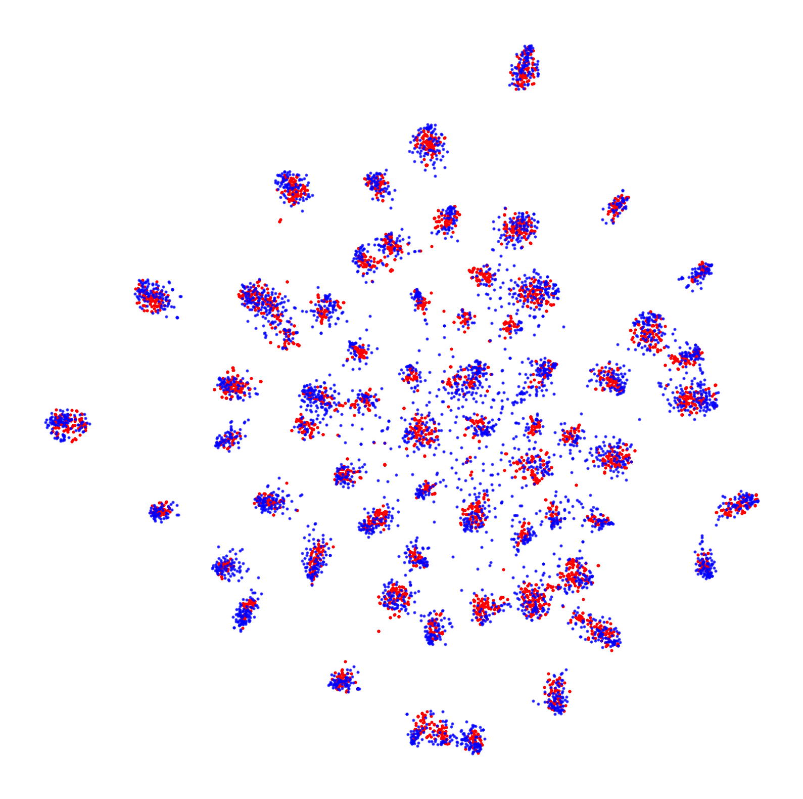
(a) MDD: Cl$\to$Rw

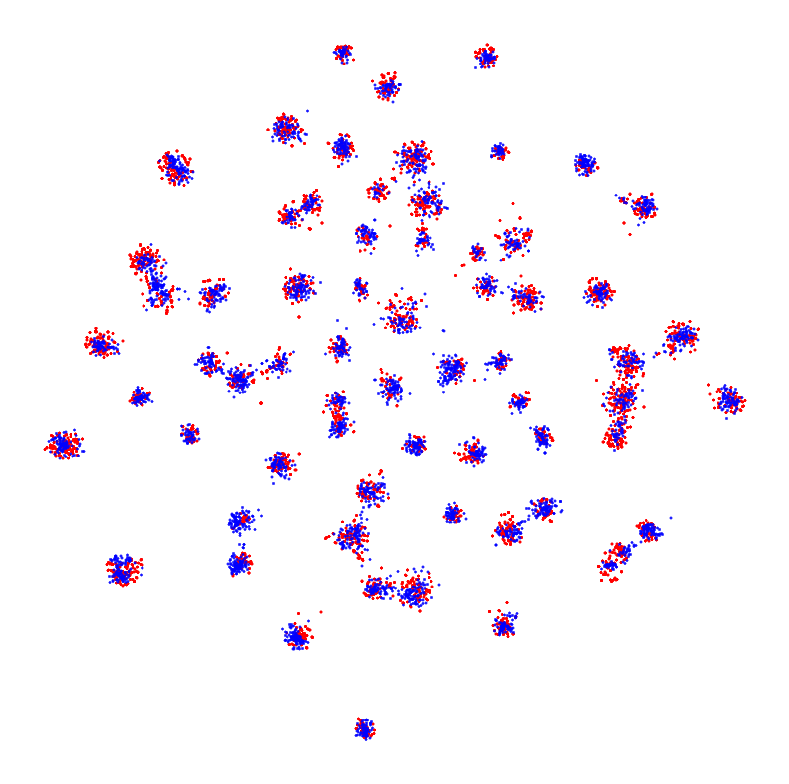
(b) MDD+SAF: Cl$\to$Rw

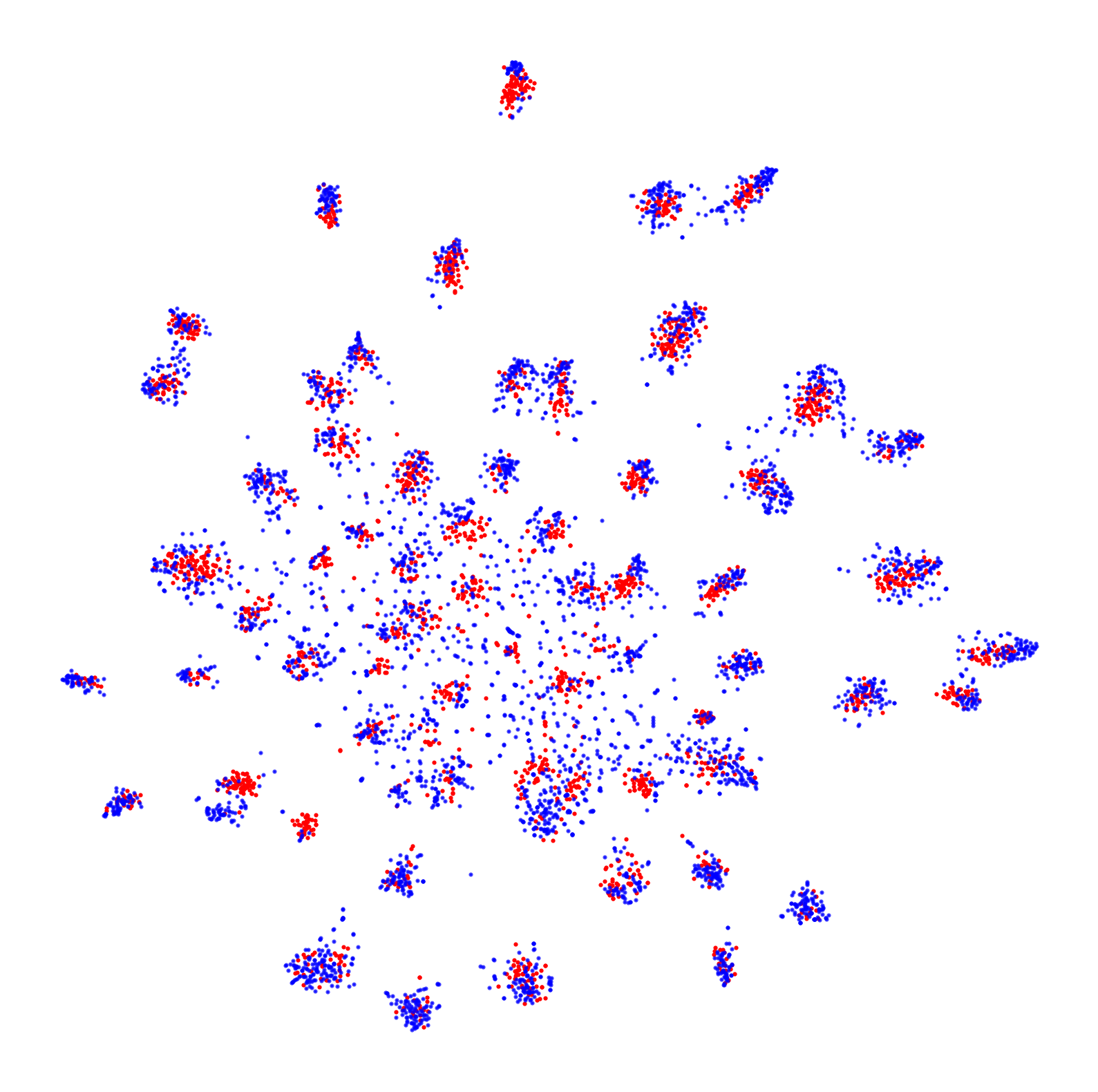
(c) MDD: Ar$\to$Pr

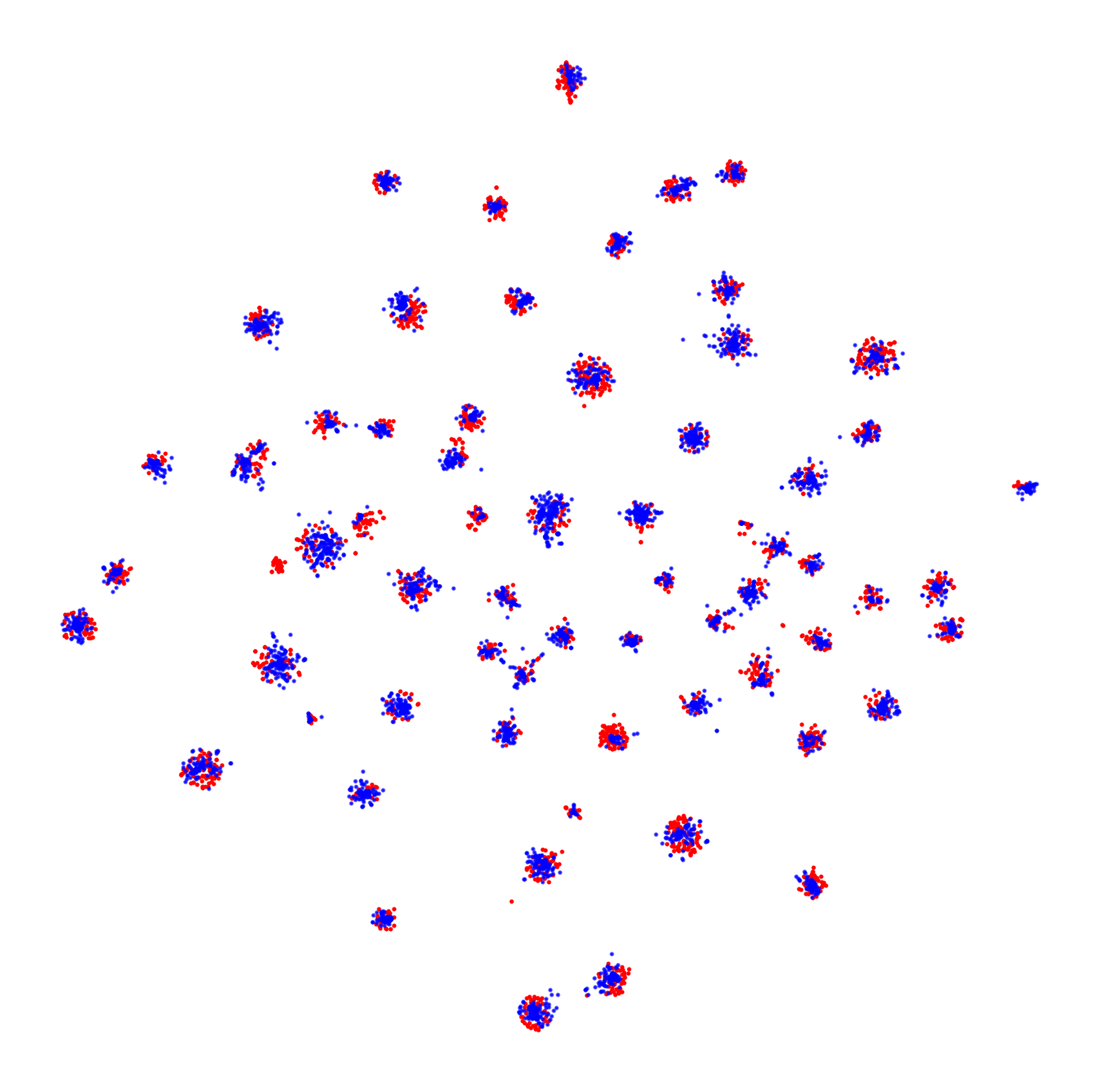
(d) MDD+SAF: Ar$\to$Pr

Figure 3: t-SNE visualizations of features extracted from Office-Home tasks. Best viewed in color. Red and blue dots represent source and target feature representations, respectively. The high-resolution version can be found in the supplementary material.

6 Conclusion

In this paper, a novel SAF algorithm is derived from the cutting-edge theories to address the unsupervised domain adaptation problem. The key idea of SAF is to distill classification-related information from target features to augment the training signals. Our SAF framework learns from input targets and guides the classifier to find reasonable class boundaries for the target distribution. Extensive experiments demonstrate the state-of-the-art performance and decent generalizability of SAF.

Appendix

6.1 Theoretical Insight:
Evolution of UDA Algorithms

In this section, we introduce the path of evolution in domain adaptation theories, along with UDA algorithms based on theoretical backgrounds over time. To summarize, we categorize the theoretical progression of domain adaptation to two stages. In each stage, researchers discover a specific issue in UDA, initially tackle with traditional statistical methods (explicit techniques), and end up with solving the problem with implicit approaches.

6.1.1 Notations

For a neural network specified for UDA tasks, denote $F$, $C$, $D$ as feature extractor, classifier, and adversarial module, respectively. The feature extractor, $F$, is a structure that distills feature representations from input images. Usually, researchers use pretrained backbones (e.g. AlexNet [23], ResNet [17]) for the extractor. The classifier, $C$, is a Multi-Layer Perceptron (MLP) that assigns class labels to input features. The adversarial module, $D$, is another MLP that is trained to regularize $F$ and $C$ through mini-max games. The adversarial module was first proposed by [10] as a domain classifier. $F,C,D$ are commonly presented in recent UDA frameworks, as the adversarial design has become pervasive among UDA algorithms.

We follow the definition of domain proposed by [2] and generalized by [20]. Given an input space $\mathcal{X}$ and a label space $\mathcal{Y}$, a domain $\mathscr{D}$ is a pair $\langle\mathcal{D},f\rangle$ consisting of a distribution $\mathcal{D}$ on $\mathcal{X}$, and a labeling function $f:\mathcal{X}\rightarrow\mathcal{Y}$. Namely, the labeling function assigns the ground-truth label $y\in\mathcal{Y}$ to each sample $x\in\mathcal{X}$.

Let $\mathscr{D}_{S}=\langle\mathcal{D}_{S},f_{S}\rangle$ denote the source domain on the input space, with domain label $\mathcal{Z}_{S}=0$. Let ($\mathcal{S}$, $\mathcal{Y}_{S}$) be the set of available labeled source samples along with empirical distribution $\widehat{\mathcal{D}}_{S}$. Let $\mathcal{F}_{S}$ be the set of feature representations extracted from the source dataset, with empirical feature distribution $\Phi_{S}$. Moreover, denote ${P}_{S}$ as the set of predicted possibility vectors from the classifier based on $\mathcal{F}_{S}$.

The symmetric (reflected) definitions on the target domain: $\mathscr{D}_{T}=\langle\mathcal{D}_{T},f_{T}\rangle$, $\mathcal{Z}_{T}=1$, $(\mathcal{T},\mathcal{Y}_{T})$, $\widehat{\mathcal{D}}_{T}$, $\mathcal{F}_{T}$, $\Phi_{T}$, ${P}_{T}$ are described in exactly the same manner as their source counterparts.

Let $\mathcal{H}$ be the hypothesis class of classifiers that maps from $\mathcal{X}$ to $\{\mathcal{Z}_{S},\mathcal{Z}_{T}\}$.

6.1.2 Settings

In Unsupervised Domain Adaptation (UDA), there are two datasets: the labeled source dataset $(\mathcal{S},\mathcal{Y}_{S})$ drawn from $\mathscr{D}_{S}$, and the unlabeled target dataset $(\mathcal{T},\varnothing)$ drawn from $\mathcal{D}_{T}$, sharing the input space $\mathcal{X}$ and the label space $\mathcal{Y}$. The crux of the UDA setting is that the discrepancy between two domains cannot be explicitly alleviated, so methods that are capable of mining underlying statistical patterns instead of merely learning from labels, are required.

6.1.3 Foundations of Domain Adaptation

We begin with the fundamental theories and basic terminologies for domain adaptation problems. For the given domains $\mathscr{D}_{S}$ and $\mathscr{D}_{T}$, we use the concept $\mathcal{H}$-divergence [2] to measure their discrepancy with respect to the hypothesis class $\mathcal{H}$:

$$d_{\mathcal{H}}(\mathcal{D}_{S},\mathcal{D}_{T})\coloneqq\\ 2\sup_{h\in\mathcal{H}}\big{|}\mathbb{P}_{\mathcal{D}_{S}}[h=0]-\mathbb{P}_{\mathcal{D}_{T}}[h=0]\big{|},$$ (12)

which can be empirically estimated if $\mathcal{H}$ is symmetric:

$$\begin{split}\hat{d}_{\mathcal{H}}(\mathcal{S},\mathcal{T})\triangleq&\\ 2\Big{(}1-\min_{h\in\mathcal{H}}&\big{[}\frac{1}{|\mathcal{S}|}\sum_{x\in h_{0}}\mathbb{1}[x\in\mathcal{S}]+\frac{1}{|\mathcal{T}|}\sum_{x\in h_{1}}\mathbb{1}[x\in\mathcal{T}]\big{]}\Big{)},\end{split}$$ (13)

where $h_{\mathcal{Z}}\coloneqq\{x\in(\mathcal{S}\cup\mathcal{T})\mid h(x)=\mathcal{Z}\}$ for $\mathcal{Z}\in\{\mathcal{Z}_{S}\coloneqq 0,\mathcal{Z}_{T}\coloneqq 1\}$, and $\mathbb{1}$ is the binary indicator function.

Intuitively, $\mathcal{H}$-divergence measures the discrepancy between two domains based on the worst domain classifier in $\mathcal{H}$. If the worst classifier $h^{-}\in\mathcal{H}$ can hardly distinguish samples from two domains, then the discrepancy between $\mathcal{S}$ and $\mathcal{T}$ would be high on $\mathcal{H}$ and vice versa.

Based on above notations, the $\mathcal{H}\Delta\mathcal{H}$-divergence [2] is defined as follows:

$$d_{\mathcal{H}\Delta\mathcal{H}}(\mathcal{D}_{S},\mathcal{D}_{T})\coloneqq\\ 2\sup_{h,h^{\prime}\in\mathcal{H}}\big{|}{\mathbb{P}}_{\mathcal{D}_{S}}[h\neq h^{\prime}]-{\mathbb{P}}_{\mathcal{D}_{T}}[h\neq h^{\prime}]\big{|}.$$ (14)

Following this definition, a powerful bounding formula for the classification error on $\mathcal{D}_{T}$ can be derived. For every $h\in\mathcal{H}$ on the target domain $\mathcal{D}_{T}$, with probability at least $1-\delta$ $(\delta>0)$:

$$\epsilon_{\mathcal{D}_{T}}(h)\leq\epsilon_{\mathcal{D}_{S}}(h)+\frac{1}{2}d_{\mathcal{H}\Delta\mathcal{H}}(\mathcal{D}_{S},\mathcal{D}_{T})+\lambda,$$ (15)

where $\lambda$ is a constant.

Hypothesis Neighborhood. The concept of hypothesis class $\mathcal{H}$ becomes confusing in above formulas. For a fixed CNN structure, the hypothesis space is unchangeable, but shrinking the discrepancy term $d_{\mathcal{H}\Delta\mathcal{H}}$ requires shifting of $\mathcal{H}$. Actually, we can regard the process of optimizing CNNs, guided by various supervisory signals (loss criterions, regularizations), as shrinking the hypothesis space. Led by supervisions, the CNNs is guided to find the optimized neighborhood, $\mathcal{H}^{*}$, in the universal hypothesis class $\mathcal{H}$, where the local $\mathcal{H}^{*}\Delta\mathcal{H}^{*}$-divergence is minimized across the universe:

$$\mathcal{H}^{*}\coloneqq\arg\min_{\mathcal{H^{\prime}}\subset\mathcal{H}}\big{[}d_{\mathcal{H^{\prime}}\Delta\mathcal{H^{\prime}}}(\mathcal{D}_{S},\mathcal{D}_{T})\big{]}.$$ (16)

In the rest of this document, the symbol $\mathcal{H}$ indicates the hypothesis neighborhood of the current classifier $h$. When designing domain adaptation algorithms, we are not interested in the universal hypothesis class, but try to discover the best optimization strategies that drive the models to reach $\mathcal{H}^{*}$.

6.1.4 Stage I: Domain Feature Alignment

After the popularization of the CNN, researchers combine traditional statistical techniques with deep CNNs [51, 30, 48, 32, 45, 29, 58] to enhance model performance in domain adaptation tasks. Generally, these works employ explicit methods to measure discrepancy between feature representations $\mathcal{F}_{S}$ and $\mathcal{F}_{T}$ (the output of the feature extractor $F$), or output probabilities ${P}_{S}$ and ${P}_{T}$ (the output of the classifier $C$). A common practice is to design a loss term based on the calculated discrepancy and to encourage the network to align all samples. Following formula 15, researchers believe that the discrepancy between $\Phi_{S}$ and $\Phi_{T}$ (the domain discrepancy among feature) greatly affects the classification accuracies. Hence, methods in this stage strive to close the gap from two directions: (1) regularize the model to ignore domain-variant features; (2) push the model escape from the suboptimal neighborhoods $\overline{\mathcal{H}^{*}}$. To sum up, in this stage, researchers try to distill the essence of explicit methods for better feature alignment across different domains.

DANN [10] is a revolutionary innovation that changes the situation. In DANN, domain-variant feature representations are no longer aligned through the assistance of explicit calculations, but implicitly achieved by training another MLP, the domain discriminator $D$. The DANN was inspired by GAN[13], where two independent deep neural networks, Generator and Discriminator, are trained together but with completely opposite goals. The Generator aims to create fake samples mimicking real samples from random gaussian noises to fool the Discriminator, while the Discriminator struggles to distinguish between real samples from datasets and fake samples generated by the Generator. Abide by the idea of Discriminator, the goal of the domain discriminator $D$ is to recognize whether the features extracted by $F$ are from the source distribution or the target counterpart. Similar to a Generator, the feature map $F$, while extracting better feature representations to aid $C$, also needs to extract domain-invariant features shared by ${\Phi}_{S}$ and ${\Phi}_{T}$, incapatiating $D$ from making correct predictions.

The invention of DANN signals a major change in the development of UDA algorithms: the alignment of domain features can finally be done in an implicit NN-styled way. Not to mention that this implicit modification outperforms existing explicit methods on popular UDA benchmarks [11].

6.1.5 Stage II: Classification Feature Alignment

As the DANN emerges, adversarial approaches become favorable among researchers, which inspires numerous adversarial UDA methods [50, 33, 42, 35, 43, 31, 26]. However, another cloud still obscure the sky of UDA researching: even though domain alignment regularizations are employed, none of the existing models can achieve the same performance on the target domain as on the source domain.

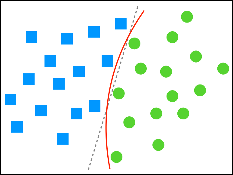
(a)

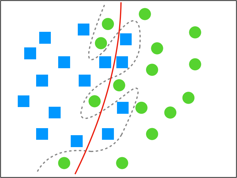
(b)

Figure 4: Illustration of discriminability. Best viewed in color. (a) shows feature distribution with decent discriminability, as the classification boundary can be closely estimated by the classifier. (b) shows the contrary, where the dashed line is the ground-truth class border, but classifier with regular capacity usually finds the solid curve as predicted broader.

Shortcomings of DANN. After a seires of formal analysis and rigorous experiments, researchers introduce two concepts that are necessary for understanding the dilemma of DANN: transferability and discriminability [5]. Transferability is an attribute indicating whether the feature representations extracted by $F$ are completely shared by both domains, i.e. $\Phi_{S}=\Phi_{T}$. Discriminability is another property referring to the easiness for a classifier to find clear class boundaries among input feature representations, as shown in Figure 4.

Formally, the DANN structure, while boost the accuracy on UDA tasks by enhancing transferability, actually misleads $F$ to extract feature representations with decreased discriminability [5]. To address this issue, multiple approaches [43, 5, 55] are attempted to explicitly increase the discriminability of the features extracted by $F$ in adversarial structures. In this stage, researchers aim to design objective functions able to lead $F$ to excavate more class-variant, or discriminative features.

We can also understand this phenomenon by investigating the theoretical supports of DANN. Since the $\mathcal{H}$-divergence (Equation 12) and the $\mathcal{H}\Delta\mathcal{H}$-divergence (Equation 14) employ the discrete 0-1 disparity as the risk criterion:

$$\epsilon_{\mathcal{D}}(h)\coloneqq\mathbb{P}_{\mathcal{D}}\big{[}\mathbb{1}[h\neq f]\big{]},$$ (17)

one can hardly generalize a reasonable scoring function for classifiers with more than two classes from them. A theoretically possible but technically impractical approach is to naively create binary classifier for every pair of classes, but this design is computationally expensive, especially for datasets with massive classes (e.g. ImageNet [7], DomainNet [36], etc.). Hence, the binary classifier $D$ can only function as a domain regularizer and cannot boost the classification accuracy.

MDD [61]. Some researchers regard such incompatibility as a gap between theories and algorithms in the field of UDA, making the optimization process extremely difficult or even impossible. To field this gap, the concept of Margin Disparity Discrepancy (MDD) [61] is formulated, which is another revolutionary theoretical innovation in the UDA research.

The MDD framework is able to implicitly align classification features between two domains with adversarial approach. MDD not only bridges the gap between existing discrete domain adaptation theories and continuous objective functions required by model training, but also implicitizes the alignment of classification features. In other words, MDD first employs the implicit approach in guiding the feature extractors to distill featuer representations with better discriminability. As a result, MDD outperforms existing methods on benchmarks [61] and again demonstrates the superiority of implicit approaches over explicit ones.

6.2 Definitions and Notations

We redefine core DA concepts to adapt the MDD system. Let $\mathscr{C}$ be the hypothesis space of classifiers that maps from the feature space $\Phi$ to $[0,1]^{|\mathcal{Y}|}$. For arbitrary $C\in\mathscr{C}$, $\phi\in\Phi$, and $y\in\mathcal{Y}$, denote $C_{y}(\phi)$ as the predicted probability for $\phi$ belonging to the class $y$, and denote $\hat{C}(\phi)$ as the predicted label for $\phi$. In addition, $\mathcal{X}$ and $\Phi$ are interchangeable in this context, as we focus on the optimization of classifiers.

Margin. Following the margin theory [22], the concept margin [61] of a classifier $C$ with respect to another classifier $C^{\prime}$ on a sample $x\in\mathcal{X}$ is defined as:

$$\rho_{C}(x,C^{\prime})\coloneqq\frac{1}{2}\big{(}C_{\hat{C^{\prime}}(x)}(x)-\max_{y\neq\hat{C^{\prime}}(x)}C_{y}(x)\big{)}.$$ (18)

Namely, the margin regards the label predicted by $C^{\prime}$ as the exemplar label, and measures the distance between the probability of the “ground-truth label” and the largest probability among the remainings.

Margin Loss. Given a task-dependent constant margin threshold (denoted as $\varrho$), we would like the margin criterion to satisfy the following properties:

• For any input, the margin loss falls in $[0,1]$.

• The loss becomes $1$ if $\rho_{C}(x,C^{\prime})$ is negative.

• The loss becomes $0$ if $\rho_{C}(x,C^{\prime})$ is larger than $\varrho$.

• The loss decreases as $\rho_{C}(x,C^{\prime})$ increases in $[0,\varrho]$.

Therefore, the fundamental margin loss [61] of a classifier $C\in\mathscr{C}$ w.r.t. another classifier $C^{\prime}\in\mathscr{C}$ on a sample $x\in\mathcal{X}$ is defined as:

$$\bar{\rho}^{(\varrho)}_{C}(x,C^{\prime})\coloneqq\\ \begin{cases}1&\text{if }\rho_{C}(x,C^{\prime})\in(-\infty,0)\\ 1-\rho_{C}(x,C^{\prime})/\varrho&\text{if }\rho_{C}(x,C^{\prime})\in[0,\varrho]\\ 0&\text{if }\rho_{C}(x,C^{\prime})\in(\varrho,\infty)\end{cases}.$$ (19)

Margin Prediction Risk. For a fixed threshold $\varrho$, define the margin prediction risk for a classifier $C$ on a domain $\mathscr{D}=\langle\mathcal{D},f\rangle$ as the following:

$$\epsilon_{\mathcal{D}}^{(\varrho)}(C)\coloneqq\mathbb{E}_{x\sim\mathcal{D}}\big{[}\bar{\rho}^{(\varrho)}_{C}(x,f)\big{]}.$$ (20)

The empirical margin prediction risk on a dataset $\mathcal{U}$ with ground-truth labeling function $f_{\mathcal{U}}$ can be calculated by:

$$\hat{\epsilon}_{\mathcal{U}}^{(\varrho)}(C)\triangleq\frac{1}{|\mathcal{U}|}\sum_{x\in\mathcal{U}}\bar{\rho}^{(\varrho)}_{C}(x,f_{\mathcal{U}}).$$ (21)

Margin Disparity. The margin disparity [61] (denoted as $\Delta$) on a domain $\langle\mathcal{D},f\rangle$ w.r.t. two classifiers $C,C^{\prime}\in\mathscr{C}$ is defined as the following:

$$\Delta_{\mathcal{D}}^{(\varrho)}(C,C^{\prime})\coloneqq\mathbb{E}_{x\sim\mathcal{D}}\big{[}\bar{\rho}^{(\varrho)}_{C}(x,C^{\prime})\big{]}.$$ (22)

And its empirical form on a dataset $\mathcal{U}$ is:

$$\hat{\Delta}_{\mathcal{U}}^{(\varrho)}(C,C^{\prime})\triangleq\frac{1}{|\mathcal{U}|}\sum_{x\in\mathcal{U}}\bar{\rho}_{C}^{(\varrho)}(x,C^{\prime}).$$ (23)

Margin Disparity Discrepancy. Fixing the threshold $\varrho$, the margin disparity discrepancy [61] (denoted as $d^{(\varrho)}$) for a classifier $C$ in the hypothesis space $\mathscr{C}$ w.r.t. domain distributions $\mathcal{D}_{S}$, $\mathcal{D}_{T}$ is defined as:

$$d_{C,\mathscr{C}}^{(\varrho)}(\mathcal{D}_{S},\mathcal{D}_{T})\coloneqq\\ 2\sup_{C^{\prime}\in\mathscr{C}}\Big{(}\Delta_{\mathcal{D}_{S}}^{(\varrho)}(C,C^{\prime})-\Delta_{\mathcal{D}_{T}}^{(\varrho)}(C,C^{\prime})\Big{)}.$$ (24)

The empirical MDD for $C$ w.r.t. source and domain datasets $\mathcal{S},\mathcal{T}$ is estimated as:

$$\hat{d}_{C,\mathscr{C}}^{(\varrho)}(\mathcal{S},\mathcal{T})\triangleq\\ 2\max_{C^{\prime}\in\mathscr{C}}\Big{(}\hat{\Delta}_{\mathcal{S}}^{(\varrho)}(C,C^{\prime})-\hat{\Delta}_{\mathcal{T}}^{(\varrho)}(C,C^{\prime})\Big{)}.$$ (25)

Error Bound w.r.t. MDD. With the equations above, we are able to deliver an error boundary of $C$ on $\mathcal{D}_{T}$, with probability at least $1-3\delta$ $(\delta>0)$:

$$\begin{split}\epsilon_{\mathcal{D}_{T}}(C)\leq\hat{\epsilon}_{\mathcal{S}}^{(\varrho)}(C)&+\hat{d}_{C,\mathscr{C}}^{(\varrho)}(\mathcal{S},\mathcal{T})+\lambda_{(\varrho,\mathscr{C},\mathcal{D}_{S},\mathcal{D}_{T})}\\ &+2\sqrt{\frac{\log\frac{2}{\delta}}{2|\mathcal{S}|}}+\sqrt{\frac{\log\frac{2}{\delta}}{2|\mathcal{T}|}}\\ &+K\Big{(}|\mathcal{Y}|,\frac{1}{\varrho},\frac{1}{\sqrt{|\mathcal{S}|}},\frac{1}{\sqrt{|\mathcal{T}|}}\Big{)},\end{split}$$ (26)

where $\lambda$ is a constant, while $K$ is a term positively related to the number of classes $|\mathcal{Y}|$ and negatively related to the margin threshold $\varrho$, and the sizes of both source and target datasets.

Hypothesis Neighborhood (MDD). As mentioned in Section 6.1.3, the concept of unchangeable hypothesis class $\mathscr{C}$ is questionable for the optimization process. In the scenario of MDD, the optimal hypothesis neighborhood $\mathscr{C}^{*}$ is a region where the local discrepancy ${d}_{C,\mathscr{C}^{*}}^{(\varrho)}(\mathcal{D}_{S},\mathcal{D}_{T})$ is the minimum across the universe:

$$\mathscr{C}^{*}\coloneqq\arg\min_{\mathscr{C}^{\prime}\subset\mathscr{C}}\big{[}\max_{C\in\mathscr{C}^{\prime}}{d}_{C,\mathscr{C}^{\prime}}^{(\varrho)}(\mathcal{D}_{S},\mathcal{D}_{T})\big{]}.$$ (27)

Similarly, we use $\mathscr{C}$ to denote the hypothesis neighborhood of the current classifier $C$.

6.3 Cross-Entropy Divergence

The cross-entropy loss, $\mathcal{L}_{\text{CEL}}$, is a pervasive loss function. For a set of logit vectors $\mathcal{P}$ with ground-truth labels $\mathcal{Q}$:

$$\mathcal{L}_{\text{CEL}}(\mathcal{P},\mathcal{Q})=\mathbb{E}_{(X,y)\in(\mathcal{P},\mathcal{Q})}\big{[}-\log[\sigma_{y}(X)]\big{]},$$ (28)

where $\sigma_{y}$ is the softmax possibility for label $y$. However, the cross-entropy loss cannot measure the divergence between two discrete distribution vectors.

Moreover, although other statistical metrics (e.g. KL-divergence, JS-divergence, etc.) provide decent discrepancy measurements, their quantitative outputs are usually too insignificant to balance the source supervision losses calculated via the cross-entropy criterion, which is unfavorable for training CNNs.

To address this disadvantage, we generalize the cross-entropy loss to composite labels by defining the cross-entropy divergence, $\mathcal{L}_{\text{CED}}$:

$$\mathcal{L}_{\text{CED}}(\mathcal{P},\mathcal{Q})=\mathbb{E}_{(X,Y)\in(\mathcal{P},\mathcal{Q})}\big{[}-Y^{T}\log[\sigma(X)]\big{]},$$ (29)

where $\mathcal{P}$ is the set of predicted logits, and $\mathcal{Q}$ is the set of composite labels.

6.4 Algorithm

The commented SAF-mixup algorithm is displayed in Algorithm 2.

Module: bottleneck $B$, classifier $C$

              SAF bottlenecks $S_{1}$, $S_{2}$

              SAF weight estimator $S_{\eta}$

Input: the set of target features $\mathcal{F}_{T}$

Output: augmented features ($\widetilde{\mathcal{F}}_{T}$, $\widetilde{\mathcal{Y}}_{\mathcal{T}}$)

1

2BEGIN:

3 # initialize output sets

4 $\widetilde{\mathcal{F}}_{T}\leftarrow\emptyset$;  $\widetilde{\mathcal{Y}}_{\mathcal{T}}\leftarrow\emptyset$

5 while $\mathcal{F}_{T}\neq\emptyset$ do

6       # draw from $\mathcal{F}_{T}$ without replacement

7       $\phi_{1},\phi_{2}\leftarrow\operatorname{RandomDrawPair}(\mathcal{F}_{T})$

8       # feed $\phi_{1},\phi_{2}$ into $S_{1},S_{2}$, respectively;

9       # then feed the sum into $S_{\eta}$ to get weight

10       $\eta\leftarrow S_{\eta}\big{(}S_{1}(\phi_{1})+S_{2}(\phi_{2})\big{)}$

11       # linearly combine $\phi_{1},\phi_{2}$ w.r.t. $\eta$

12       $\tilde{\phi}\leftarrow\eta\phi_{1}+(1-\eta)\phi_{2}$;

13       # get pseudo-labels for the pair

14       $\hat{y}_{1}\leftarrow C\circ B(\phi_{1});\>\hat{y}_{2}\leftarrow C\circ B(\phi_{2})$

15       # similar for $\hat{y}_{1},\hat{y}_{2}$

16       $\tilde{y}\leftarrow\eta\hat{y}_{1}+(1-\eta)\hat{y}_{2}$

17       # update $\widetilde{\mathcal{F}}_{T}$ and $\widetilde{\mathcal{Y}}_{\mathcal{T}}$

18       $\widetilde{\mathcal{F}}_{T}\leftarrow\widetilde{\mathcal{F}}_{T}\cup\{\tilde{\phi}\}$;  $\widetilde{\mathcal{Y}}_{\mathcal{T}}\leftarrow\widetilde{\mathcal{Y}}_{\mathcal{T}}\cup\{\tilde{y}\}$

19      

20 end while

END.

Algorithm 2 SAF-mixup

The training scheme for the complete SAF framework is shown in Algorithm 3.

6.5 Implementation Details

6.5.1 Network Structures

The network structure designed for experiments is built upon source codes of MDD [61] and of ImA [20]. The source code can be found in our supplementary materials.

The feature extractor $F$ is a ResNet50 [17] pre-trained on the ImageNet [7], following the commonly-used UDA training protocol [10, 31].

The bottleneck $B$ uses the following structure:

• Fully-Connected Layer (2048$\to$1024)

• Batch Normalization Layer

• ReLU Layer

• Dropout Layer (50%)

to filter input features.

The classifier $C$ and the adversarial module $D$ shares the same architecture in the MDD structure, where $D$ is able to regularize $F$ for extraction of transferable as well as discriminative features:

• Fully-Connected Layer (1024$\to$1024)

• ReLU Layer

• Dropout Layer (50%)

• Fully-Connected Layer (1024$\to$$|\mathcal{Y}|$)

where $|\mathcal{Y}|$ is the number of classes.

SAF bottlenecks $S_{1},S_{2}$ use relatively simple structure to process feature representations from $F$:

• Fully-Connected Layer (2048$\to$384)

• ReLU Layer

while the SAF weight estimator consists of:

• Fully-Connected Layer (384$\to$1)

• Sigmoid Layer

which yields a weight $\eta\in(0,1)$.

Module: feature map $F$, bottleneck $B$

              classifier $C$, adversarial module $D$

              SAF mixup module $M$

Parameter: learning rate $\lambda$

Input: source dataset $(\mathcal{S},\mathcal{Y}_{S})$

           target dataset $(\mathcal{T},\emptyset)$

1

2BEGIN:

3 # source label prediction objective

4 $\mathcal{P}_{S}\leftarrow[C\circ B\circ F](\mathcal{S})$

5 $\varepsilon_{C}\leftarrow L_{C}(\mathcal{P}_{S},\mathcal{Y}_{S})$

6 # adversarial domain adaptation objective

7 $\varepsilon_{D}\leftarrow L_{D}(F,B,D,C,\mathcal{S},\mathcal{T})$

8 # SAF-supervision objective

9 $\mathcal{F}_{T}\leftarrow F(\mathcal{T})$

10 $\widetilde{\mathcal{F}}_{T},\widetilde{\mathcal{Y}}_{T}\leftarrow M(\mathcal{F}_{T})$

11 $\varepsilon_{M}\leftarrow L_{M}(\widetilde{\mathcal{F}}_{T},\widetilde{\mathcal{Y}}_{T})$

12 # backpropagation (denoted as $\leftarrow^{*}$)

13 $F,M,B,C\leftarrow^{*}-\lambda(\varepsilon_{C}+\lambda_{D}\varepsilon_{D}+\lambda_{M}\varepsilon_{M})$

14 $D\leftarrow^{*}\lambda\varepsilon_{D}$

END.

Algorithm 3 SAF Training Algorithm

6.5.2 Hyperparameters

The GRL [10] weight $\lambda_{D}$ is initially set to $0$ and gradually increases to $0.1$, with the increasing function:

$$\lambda_{D}(t)=0.1\tanh\frac{10t}{\mathbf{T}},$$ (30)

where $t$ is the current iteration number, and $\mathbf{T}=10^{5}$ is the total training iteration.

Similarly, the SAF mixup weight $\lambda_{M}$ increases from $0$ to $0.1$ in a slower pace:

$$\lambda_{M}(t)=0.1\tanh\frac{5t}{\mathbf{T}}.$$ (31)

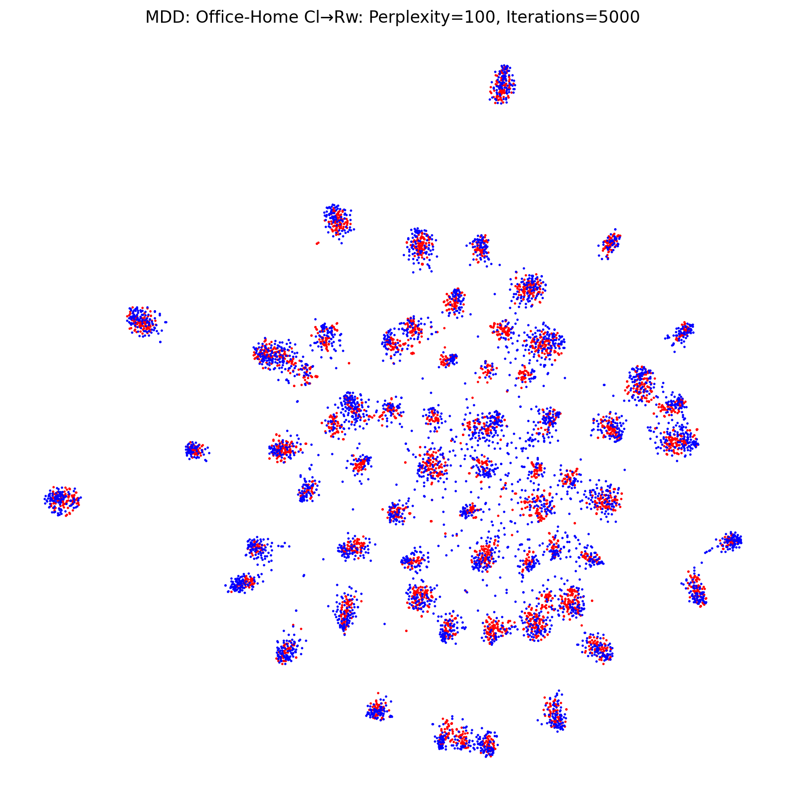
(a) MDD: Cl$\to$Rw

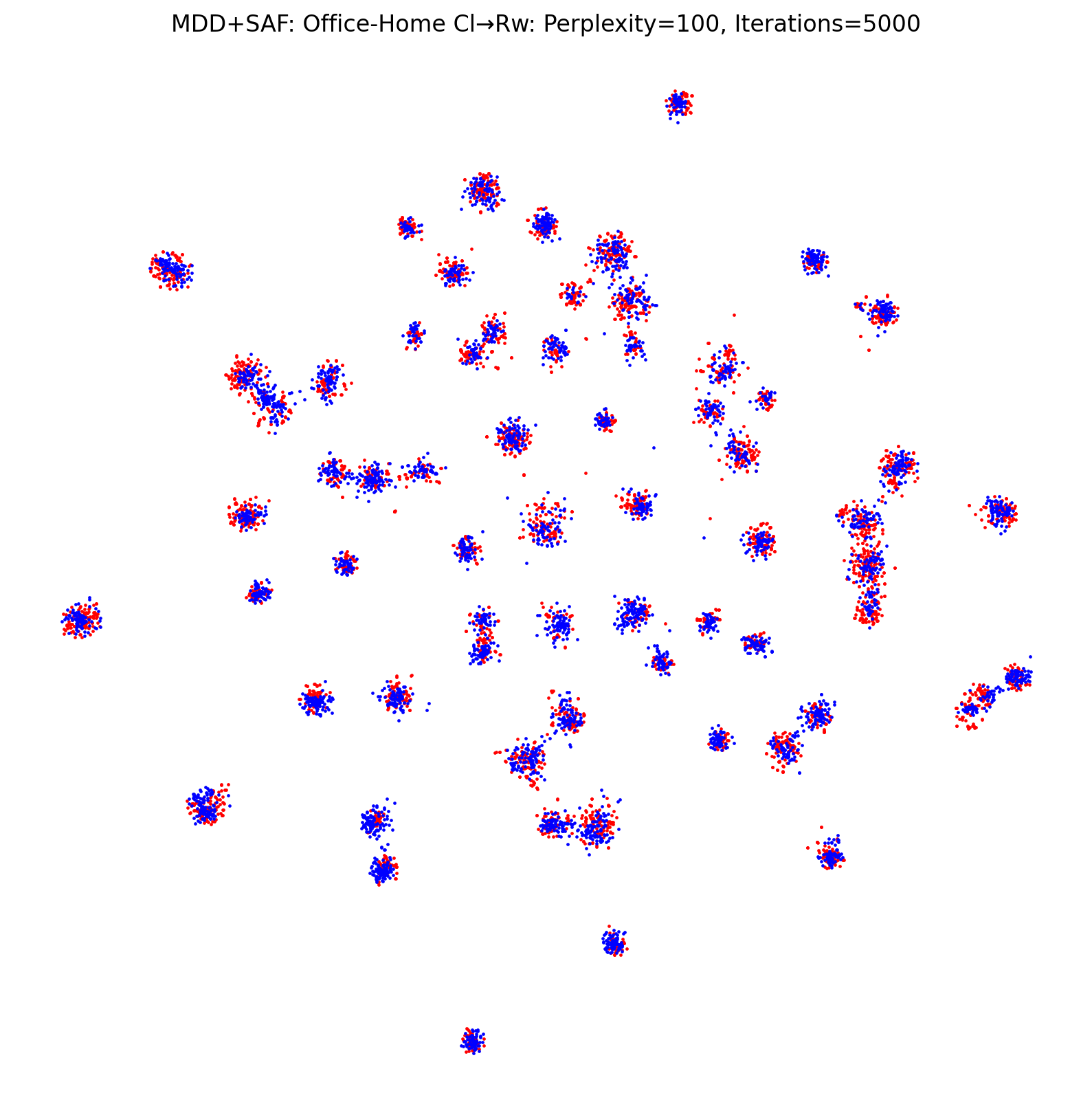
(b) MDD+SAF: Cl$\to$Rw

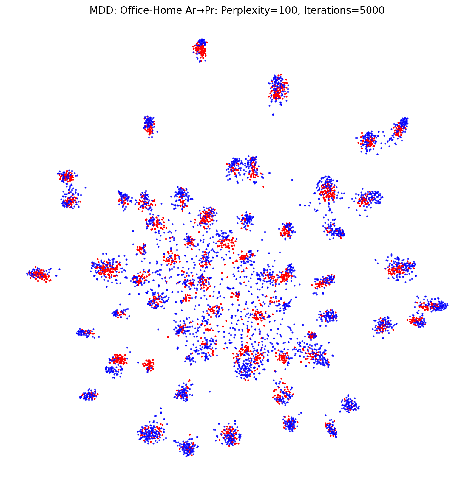
(c) MDD: Ar$\to$Pr

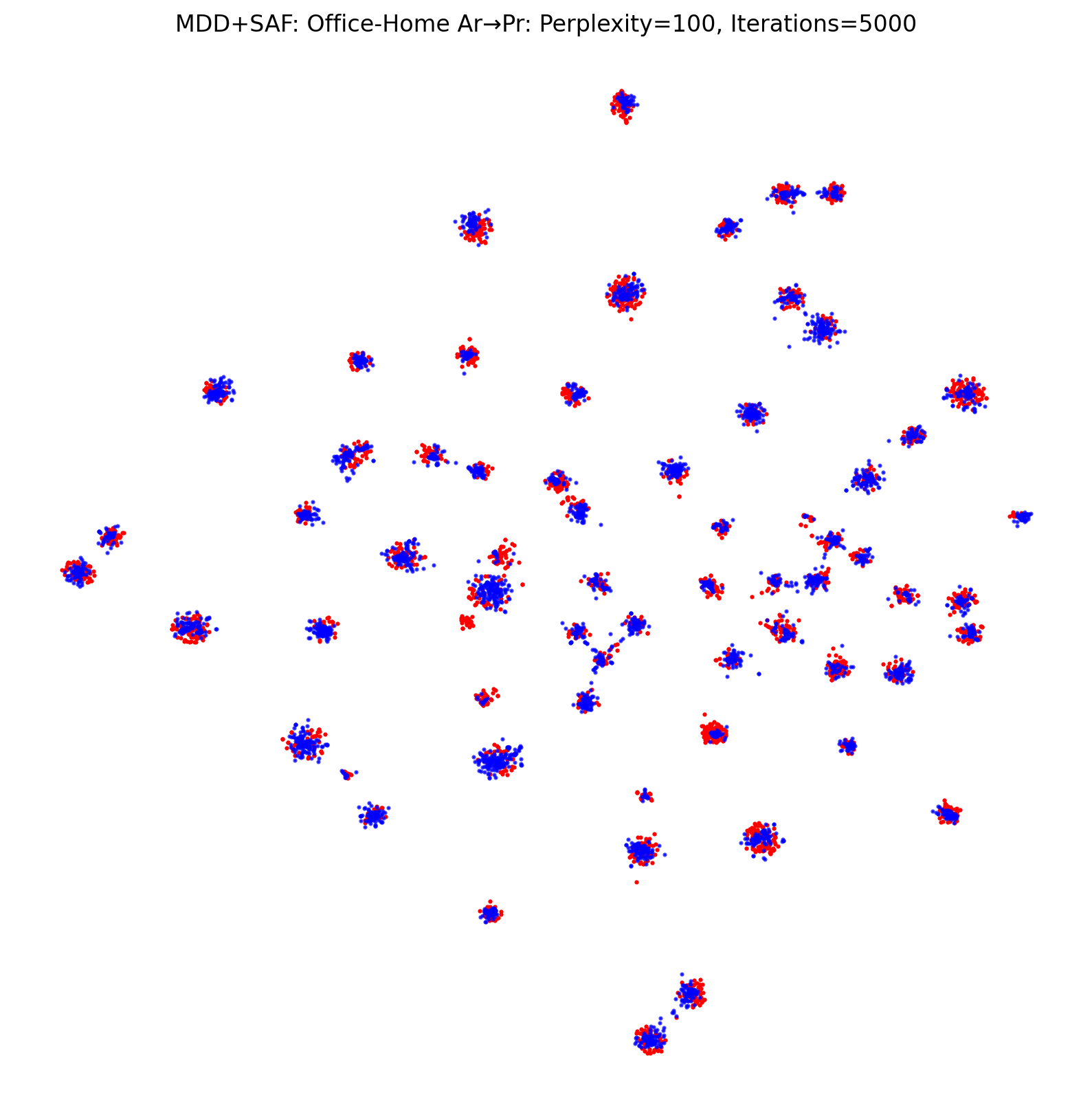
(d) MDD+SAF: Ar$\to$Pr

Figure 5: t-SNE visualizations for features extracted from Office-Home Cl$\to$Rw and Ar$\to$Pr tasks. Best viewed in color. Red and blue dots represent source and target feature representations, respectively.

6.6 Visualizations

Two sets of t-SNE visualizations [52] are shown in Figure 5. Figure 5(a) and 5(b) displays the features extracted from the Office-Home Cl$\to$Rw task. Figure 3(c) and 5(d) displays the features extracted from the Office-Home Ar$\to$Pr task.

The visualization comparison between MDD and SAF shows that the SAF framework greatly improves feature clustering and semantic transferring between two domains.

References

- [1] W. H. Beluch, T. Genewein, A. Nurnberger, and J. M. Kohler. The power of ensembles for active learning in image classification. In 2018 IEEE/CVF Conference on Computer Vision and Pattern Recognition, pages 9368–9377, June 2018.
- [2] Shai Ben-David, John Blitzer, Koby Crammer, Alex Kulesza, Fernando Pereira, and Jennifer Wortman Vaughan. A theory of learning from different domains. Mach. Learn., 79(1–2):151–175, May 2010.
- [3] Shai Ben-David, John Blitzer, Koby Crammer, and Fernando Pereira. Analysis of representations for domain adaptation. In B. Schölkopf, J. Platt, and T. Hoffman, editors, Advances in Neural Information Processing Systems, volume 19. MIT Press, 2007.
- [4] Lukas Bossard, Matthieu Guillaumin, and Luc Van Gool. Food-101 – mining discriminative components with random forests. In European Conference on Computer Vision, 2014.
- [5] Xinyang Chen, Sinan Wang, Mingsheng Long, and Jianmin Wang. Transferability vs. discriminability: Batch spectral penalization for adversarial domain adaptation. In Kamalika Chaudhuri and Ruslan Salakhutdinov, editors, Proceedings of the 36th International Conference on Machine Learning, volume 97 of Proceedings of Machine Learning Research, pages 1081–1090. PMLR, 09–15 Jun 2019.
- [6] David A. Cohn, Zoubin Ghahramani, and Michael I. Jordan. Active learning with statistical models. J. Artif. Int. Res., 4(1):129–145, Mar. 1996.
- [7] J. Deng, W. Dong, R. Socher, L.-J. Li, K. Li, and L. Fei-Fei. ImageNet: A Large-Scale Hierarchical Image Database. In CVPR09, 2009.
- [8] Zhijie Deng, Yucen Luo, and Jun Zhu. Cluster alignment with a teacher for unsupervised domain adaptation. In Proceedings of the IEEE/CVF International Conference on Computer Vision (ICCV), October 2019.
- [9] Yarin Gal, Riashat Islam, and Zoubin Ghahramani. Deep Bayesian active learning with image data. In Doina Precup and Yee Whye Teh, editors, Proceedings of the 34th International Conference on Machine Learning, volume 70 of Proceedings of Machine Learning Research, pages 1183–1192, International Convention Centre, Sydney, Australia, 06–11 Aug 2017. PMLR.
- [10] Yaroslav Ganin and Victor Lempitsky. Unsupervised domain adaptation by backpropagation. In Francis Bach and David Blei, editors, Proceedings of the 32nd International Conference on Machine Learning, volume 37 of Proceedings of Machine Learning Research, pages 1180–1189, Lille, France, 07–09 Jul 2015. PMLR.
- [11] Yaroslav Ganin, Evgeniya Ustinova, Hana Ajakan, Pascal Germain, Hugo Larochelle, François Laviolette, Mario Marchand, and Victor Lempitsky. Domain-adversarial training of neural networks. J. Mach. Learn. Res., 17(1):2096–2030, Jan. 2016.
- [12] B. Gong, Y. Shi, F. Sha, and K. Grauman. Geodesic flow kernel for unsupervised domain adaptation. In 2012 IEEE Conference on Computer Vision and Pattern Recognition, pages 2066–2073, June 2012.
- [13] Ian Goodfellow, Jean Pouget-Abadie, Mehdi Mirza, Bing Xu, David Warde-Farley, Sherjil Ozair, Aaron Courville, and Yoshua Bengio. Generative adversarial nets. In Z. Ghahramani, M. Welling, C. Cortes, N. Lawrence, and K. Q. Weinberger, editors, Advances in Neural Information Processing Systems, volume 27. Curran Associates, Inc., 2014.
- [14] Yves Grandvalet and Yoshua Bengio. Semi-supervised learning by entropy minimization. In Proceedings of the 17th International Conference on Neural Information Processing Systems, NIPS’04, page 529–536, Cambridge, MA, USA, 2004. MIT Press.
- [15] Bo Han, Quanming Yao, Tongliang Liu, Gang Niu, Ivor W. Tsang, James T. Kwok, and Masashi Sugiyama. A survey of label-noise representation learning: Past, present and future, 2021.
- [16] Jiangfan Han, Ping Luo, and Xiaogang Wang. Deep self-learning from noisy labels. In Proceedings of the IEEE/CVF International Conference on Computer Vision (ICCV), October 2019.
- [17] K. He, X. Zhang, S. Ren, and J. Sun. Deep residual learning for image recognition. In 2016 IEEE Conference on Computer Vision and Pattern Recognition (CVPR), pages 770–778, June 2016.
- [18] Andrew G. Howard, Menglong Zhu, Bo Chen, Dmitry Kalenichenko, Weijun Wang, Tobias Weyand, Marco Andreetto, and Hartwig Adam. Mobilenets: Efficient convolutional neural networks for mobile vision applications, 2017.
- [19] L. Hu, M. Kan, S. Shan, and X. Chen. Duplex generative adversarial network for unsupervised domain adaptation. In 2018 IEEE/CVF Conference on Computer Vision and Pattern Recognition, pages 1498–1507, June 2018.
- [20] Xiang Jiang, Qicheng Lao, Stan Matwin, and Mohammad Havaei. Implicit class-conditioned domain alignment for unsupervised domain adaptation. In Hal Daumé III and Aarti Singh, editors, Proceedings of the 37th International Conference on Machine Learning, volume 119 of Proceedings of Machine Learning Research, pages 4816–4827. PMLR, 13–18 Jul 2020.
- [21] A. J. Joshi, F. Porikli, and N. Papanikolopoulos. Multi-class active learning for image classification. In 2009 IEEE Conference on Computer Vision and Pattern Recognition, pages 2372–2379, June 2009.
- [22] V. Koltchinskii and D. Panchenko. Empirical Margin Distributions and Bounding the Generalization Error of Combined Classifiers. The Annals of Statistics, 30(1):1 – 50, 2002.
- [23] Alex Krizhevsky, Ilya Sutskever, and Geoffrey E Hinton. Imagenet classification with deep convolutional neural networks. In F. Pereira, C. J. C. Burges, L. Bottou, and K. Q. Weinberger, editors, Advances in Neural Information Processing Systems, volume 25. Curran Associates, Inc., 2012.
- [24] Y. LeCun, B. Boser, J. S. Denker, D. Henderson, R. E. Howard, W. Hubbard, and L. D. Jackel. Backpropagation applied to handwritten zip code recognition. Neural Computation, 1(4):541–551, Dec 1989.
- [25] Kuang-Huei Lee, Xiaodong He, Lei Zhang, and Linjun Yang. Cleannet: Transfer learning for scalable image classifier training with label noise. In Proceedings of the IEEE Conference on Computer Vision and Pattern Recognition (CVPR), 2018.
- [26] S. Lee, D. Kim, N. Kim, and S. Jeong. Drop to adapt: Learning discriminative features for unsupervised domain adaptation. In 2019 IEEE/CVF International Conference on Computer Vision (ICCV), pages 91–100, Oct 2019.
- [27] Rui Li, Qianfen Jiao, Wenming Cao, Hau-San Wong, and Si Wu. Model adaptation: Unsupervised domain adaptation without source data. In Proceedings of the IEEE/CVF Conference on Computer Vision and Pattern Recognition (CVPR), June 2020.
- [28] Wen Li, Limin Wang, Wei Li, Eirikur Agustsson, and Luc Van Gool. Webvision database: Visual learning and understanding from web data, 2017.
- [29] Jian Liang, Ran He, Zhenan Sun, and Tieniu Tan. Distant supervised centroid shift: A simple and efficient approach to visual domain adaptation. In Proceedings of the IEEE/CVF Conference on Computer Vision and Pattern Recognition (CVPR), June 2019.
- [30] Mingsheng Long, Yue Cao, Jianmin Wang, and Michael I. Jordan. Learning transferable features with deep adaptation networks. In Proceedings of the 32nd International Conference on International Conference on Machine Learning - Volume 37, ICML’15, page 97–105. JMLR.org, 2015.
- [31] Mingsheng Long, ZHANGJIE CAO, Jianmin Wang, and Michael I Jordan. Conditional adversarial domain adaptation. In S. Bengio, H. Wallach, H. Larochelle, K. Grauman, N. Cesa-Bianchi, and R. Garnett, editors, Advances in Neural Information Processing Systems, volume 31. Curran Associates, Inc., 2018.
- [32] Mingsheng Long, Han Zhu, Jianmin Wang, and Michael I. Jordan. Unsupervised domain adaptation with residual transfer networks. In Proceedings of the 30th International Conference on Neural Information Processing Systems, NIPS’16, page 136–144, Red Hook, NY, USA, 2016. Curran Associates Inc.
- [33] Mingsheng Long, Han Zhu, Jianmin Wang, and Michael I. Jordan. Deep transfer learning with joint adaptation networks. In Doina Precup and Yee Whye Teh, editors, Proceedings of the 34th International Conference on Machine Learning, volume 70 of Proceedings of Machine Learning Research, pages 2208–2217, International Convention Centre, Sydney, Australia, 06–11 Aug 2017. PMLR.
- [34] Xudong Mao, Yun Ma, Zhenguo Yang, Yangbin Chen, and Qing Li. Virtual mixup training for unsupervised domain adaptation. arXiv preprint arXiv:1905.04215, 2019.
- [35] Zhongyi Pei, Zhangjie Cao, Mingsheng Long, and Jianmin Wang. Multi-adversarial domain adaptation. In Sheila A. McIlraith and Kilian Q. Weinberger, editors, Proceedings of the Thirty-Second AAAI Conference on Artificial Intelligence, (AAAI-18), the 30th innovative Applications of Artificial Intelligence (IAAI-18), and the 8th AAAI Symposium on Educational Advances in Artificial Intelligence (EAAI-18), New Orleans, Louisiana, USA, February 2-7, 2018, pages 3934–3941. AAAI Press, 2018.
- [36] Xingchao Peng, Qinxun Bai, Xide Xia, Zijun Huang, Kate Saenko, and Bo Wang. Moment matching for multi-source domain adaptation. In Proceedings of the IEEE International Conference on Computer Vision, pages 1406–1415, 2019.
- [37] Xingchao Peng, Ben Usman, Neela Kaushik, Judy Hoffman, Dequan Wang, and Kate Saenko. Visda: The visual domain adaptation challenge, 2017.
- [38] Xiaojiang Peng, Kai Wang, Zhaoyang Zeng, Qing Li, Jianfei Yang, and Yu Qiao. Suppressing mislabeled data via grouping and self-attention. In Andrea Vedaldi, Horst Bischof, Thomas Brox, and Jan-Michael Frahm, editors, Computer Vision – ECCV 2020, pages 786–802, Cham, 2020. Springer International Publishing.
- [39] B. T. Polyak and A. B. Juditsky. Acceleration of stochastic approximation by averaging. SIAM J. Control Optim., 30(4):838–855, July 1992.
- [40] D. E. Rumelhart and J. L. McClelland. Learning Internal Representations by Error Propagation, pages 318–362. MIT Press, 1987.
- [41] Kate Saenko, Brian Kulis, Mario Fritz, and Trevor Darrell. Adapting visual category models to new domains. In Proceedings of the 11th European Conference on Computer Vision: Part IV, ECCV’10, page 213–226, Berlin, Heidelberg, 2010. Springer-Verlag.
- [42] Kuniaki Saito, Yoshitaka Ushiku, and Tatsuya Harada. Asymmetric tri-training for unsupervised domain adaptation. In Doina Precup and Yee Whye Teh, editors, Proceedings of the 34th International Conference on Machine Learning, volume 70 of Proceedings of Machine Learning Research, pages 2988–2997, International Convention Centre, Sydney, Australia, 06–11 Aug 2017. PMLR.
- [43] Kuniaki Saito, Kohei Watanabe, Yoshitaka Ushiku, and Tatsuya Harada. Maximum classifier discrepancy for unsupervised domain adaptation. In Proceedings of the IEEE Conference on Computer Vision and Pattern Recognition (CVPR), June 2018.
- [44] S. Sankaranarayanan, Y. Balaji, C. D. Castillo, and R. Chellappa. Generate to adapt: Aligning domains using generative adversarial networks. In 2018 IEEE/CVF Conference on Computer Vision and Pattern Recognition, pages 8503–8512, June 2018.
- [45] Rui Shu, Hung H. Bui, Hirokazu Narui, and Stefano Ermon. A DIRT-T approach to unsupervised domain adaptation. In 6th International Conference on Learning Representations, ICLR 2018, Vancouver, BC, Canada, April 30 - May 3, 2018, Conference Track Proceedings. OpenReview.net, 2018.
- [46] Hwanjun Song, Minseok Kim, and Jae-Gil Lee. SELFIE: Refurbishing unclean samples for robust deep learning. In Kamalika Chaudhuri and Ruslan Salakhutdinov, editors, Proceedings of the 36th International Conference on Machine Learning, volume 97 of Proceedings of Machine Learning Research, pages 5907–5915. PMLR, 09–15 Jun 2019.
- [47] Hwanjun Song, Minseok Kim, Dongmin Park, and Jae-Gil Lee. Learning from noisy labels with deep neural networks: A survey, 2020.
- [48] Saenko K. Sun B. Deep coral: Correlation alignment for deep domain adaptation. ECCV 2016. Lecture Notes in Computer Science, vol 9915., 9915, 2016.
- [49] Ilya Sutskever, James Martens, George Dahl, and Geoffrey Hinton. On the importance of initialization and momentum in deep learning. In Sanjoy Dasgupta and David McAllester, editors, Proceedings of the 30th International Conference on Machine Learning, volume 28 of Proceedings of Machine Learning Research, pages 1139–1147, Atlanta, Georgia, USA, 17–19 Jun 2013. PMLR.
- [50] E. Tzeng, J. Hoffman, K. Saenko, and T. Darrell. Adversarial discriminative domain adaptation. In 2017 IEEE Conference on Computer Vision and Pattern Recognition (CVPR), pages 2962–2971, July 2017.
- [51] Eric Tzeng, Judy Hoffman, Ning Zhang, Kate Saenko, and Trevor Darrell. Deep domain confusion: Maximizing for domain invariance, 2014.
- [52] Laurens van der Maaten and Geoffrey Hinton. Visualizing data using t-sne. Journal of Machine Learning Research, 9(86):2579–2605, 2008.
- [53] Hemanth Venkateswara, Jose Eusebio, Shayok Chakraborty, and Sethuraman Panchanathan. Deep hashing network for unsupervised domain adaptation. In Proceedings of the IEEE Conference on Computer Vision and Pattern Recognition, pages 5018–5027, 2017.
- [54] Zhen Wang, Guosheng Hu, and Qinghua Hu. Training noise-robust deep neural networks via meta-learning. In Proceedings of the IEEE/CVF Conference on Computer Vision and Pattern Recognition (CVPR), June 2020.
- [55] Zeya Wang, Baoyu Jing, Yang Ni, Nanqing Dong, Pengtao Xie, and Eric P. Xing. Adversarial domain adaptation being aware of class relationships, 2020.
- [56] Yuan Wu, Diana Inkpen, and Ahmed El-Roby. Dual mixup regularized learning for adversarial domain adaptation. In Andrea Vedaldi, Horst Bischof, Thomas Brox, and Jan-Michael Frahm, editors, Computer Vision – ECCV 2020, pages 540–555, Cham, 2020. Springer International Publishing.
- [57] Tong Xiao, Tian Xia, Yi Yang, Chang Huang, and Xiaogang Wang. Learning from massive noisy labeled data for image classification. In CVPR, 2015.
- [58] Ruijia Xu, Guanbin Li, Jihan Yang, and Liang Lin. Larger norm more transferable: An adaptive feature norm approach for unsupervised domain adaptation. In The IEEE International Conference on Computer Vision (ICCV), October 2019.
- [59] Hongyi Zhang, Moustapha Cissé, N. Yann Dauphin, and David Lopez-Paz. mixup: Beyond empirical risk minimization. international conference on learning representations, 2018.
- [60] Weihe Zhang, Yali Wang, and Yu Qiao. Metacleaner: Learning to hallucinate clean representations for noisy-labeled visual recognition. In Proceedings of the IEEE/CVF Conference on Computer Vision and Pattern Recognition (CVPR), June 2019.
- [61] Yuchen Zhang, Tianle Liu, Mingsheng Long, and Michael Jordan. Bridging theory and algorithm for domain adaptation. In Kamalika Chaudhuri and Ruslan Salakhutdinov, editors, Proceedings of the 36th International Conference on Machine Learning, volume 97 of Proceedings of Machine Learning Research, pages 7404–7413. PMLR, 09–15 Jun 2019.
- [62] Yabin Zhang, Hui Tang, Kui Jia, and Mingkui Tan. Domain-symmetric networks for adversarial domain adaptation. In Proceedings of the IEEE Conference on Computer Vision and Pattern Recognition, pages 5031–5040, 2019.
- [63] Z. Zhang, H. Zhang, S. Ö. Arik, H. Lee, and T. Pfister. Distilling effective supervision from severe label noise. In 2020 IEEE/CVF Conference on Computer Vision and Pattern Recognition (CVPR), pages 9291–9300, June 2020.
- [64] Li Zhong, Zhen Fang, Feng Liu, Jie Lu, Bo Yuan, and Guangquan Zhang. How does the combined risk affect the performance of unsupervised domain adaptation approaches? CoRR, abs/2101.01104, 2021.