Supplementary materials for:
“Limits on axions and axionlike particles within the axion window using a spin-based amplifier”

I Spin sensor

In this section, we describe the details of spin-based amplifier (spin sensor), which has been recently demonstrated in Refs. [1, 2]. In this work, we use a spin-based amplifier to search for the exotic spin-dependent interaction $V_{pp}$ described in Ref. [3] (equivalently $V_{3}$ in Ref. [4]). As shown in Sec. I, the exotic interaction $V_{pp}$ can generate an oscillating pseudomagnetic field on the spin-based amplifier and can be amplified by it by a factor of more than 40.

I.1 Schematic of the spin-based amplifier

The details of the experimental apparatus are shown in Fig. S1. The spin-based amplifier uses a 0.5 cm³ cubic vapor cell (cell 1) containing 5 torr of isotopically enriched ¹²⁹Xe, 250 torr N₂ as buffer gas, and a droplet (several milligrams) of isotopically enriched ⁸⁷Rb. ⁸⁷Rb atoms are polarized by a circularly polarized laser at 795 nm and probed by a linearly polarized laser blue-detuned 110 GHz from the D2 transition at 780 nm. ¹²⁹Xe spins are polarized by spin-exchange collisions with polarized ⁸⁷Rb atoms. In order to match the oscillation frequency $\nu$ of the pseudomagnetic field generated by the exotic interaction $V_{pp}$ (see the details of spin source in Sec. II and the pseudomagnetic field in Sec. III), the ¹²⁹Xe Larmor frequency $\nu_{0}$ is tuned to $\nu$ by adjusting the bias magnetic field $B_{z}^{0}$ applied with a set of Helmholtz coils [see Fig. S1(b)]. In the resonant case ($\nu_{0}\approx\nu$), the polarized ¹²⁹Xe spins are tilted away from the $z$ axis, and then generate oscillating transverse magnetization. Due to the Fermi-contact interactions between ⁸⁷Rb and ¹²⁹Xe spins, the ¹²⁹Xe transverse magnetization produces an effective oscillating field on ⁸⁷Rb atoms, which functions as a magnetometer to in situ measure this field [1, 2]. In particular, we experimentally demonstrate that the effective field strength is much larger than the pseudomagnetic field strength by a factor of about 40 (see the main text). As a result, ¹²⁹Xe spins act as a transducer converting the pseudomagnetic field into the effective magnetic field probed with ⁸⁷Rb spins. We present the experimental calibration for the spin-based amplifier in Sec. V.1.

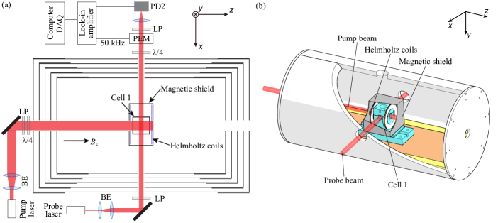
Figure S1: Experimental setup of the spin sensor. (a) Two-dimensional diagram of the spin-based amplifier as spin sensor. A vapor cell (cell 1) contains spatially overlapping ensembles of ¹²⁹Xe and ⁸⁷Rb and is heated to 165^∘C. A circularly polarized pump laser polarizes ⁸⁷Rb atoms along $z$. ¹²⁹Xe spins are polarized with polarized ⁸⁷Rb atoms through spin-exchange collisions. A resonant pseudomagnetic field can be amplified by ¹²⁹Xe spins, which produce an effective magnetic field $\textbf{B}_{\textrm{eff}}^{n}$ measured in situ with ⁸⁷Rb atoms. BE, beam expander; LP, linear polarizer; $\lambda/4$, quarter-wave plate; PD, photodiode; PEM, photoelastic modulator; DAQ, data acquisition. (b) Three-dimensional diagram of the spin-based amplifier.

I.2 Analysis of spin-based amplifier

The exotic spin-spin interactions $V_{pp}$ mediated by axions can produce an pseudomagnetic field (see Sec. III). In the following, we present the theoretical analysis of the response of the spin-based amplifier to this field. We also perform experimental calibrations by applying an oscillating field to simulate the pseudomagnetic field.

The Fermi-contact interaction between them introduces an effective magnetic field [5]

$$\textbf{B}^{e,n}_{\textrm{eff}}=\beta M_{0}^{e,n}\textbf{P}^{e,n},$$ (S1)

where $\textbf{B}^{e}_{\textrm{eff}}$ ($\textbf{B}^{n}_{\textrm{eff}}$) represents the effective magnetic field experienced by ¹²⁹Xe (⁸⁷Rb) spins, $\beta=8\pi\kappa_{0}/3$, $\kappa_{0}$ is the enhancement factor of the Fermi-contact interaction, $M_{0}^{e}$ ($M_{0}^{n}$) is the maximum magnetization of ⁸⁷Rb electron (¹²⁹Xe nucleus), and $\textbf{P}^{e}$ ($\textbf{P}^{n}$) is the polarization of ⁸⁷Rb electron (¹²⁹Xe nucleus). In contrast to the ”self-compensating” comagnetometers where ⁸⁷Rb and ¹²⁹Xe spins are strongly coupled with each other, the spin-based amplifier operates under a relatively larger bias field $B_{z}^{0}$, leading to the weak coupling between ⁸⁷Rb and ¹²⁹Xe spins. The effective field $\textbf{B}^{e}_{\textrm{eff}}$ of electron spins is similar as a weak static field along $z$ that slightly shifts the ¹²⁹Xe Larmor frequency. The effective field $\textbf{B}^{n}_{\textrm{eff}}$ of nuclear spins with the enhancement of the pseudomagnetic field is measured in situ with the ⁸⁷Rb spins.

The resonant response of the spin-based amplifier to an oscillating magnetic field, for example, $\textbf{B}_{\textrm{ac}}^{\textrm{exo}}=B_{\textrm{ac}}^{\textrm{exo}}\cos(2\pi\nu t)\hat{\bm{y}}$, can be described with the Bloch equation

$$\frac{\partial\textbf{P}^{n}}{\partial t}=\gamma_{n}({B}_{z}\hat{\bm{z}}+\textbf{B}_{\textrm{ac}}^{\textrm{exo}})\times\textbf{P}^{n}+\frac{P^{n}_{0}\hat{\bm{z}}-\textbf{P}^{n}}{\{T_{2n},T_{2n},T_{1n}\}},$$ (S2)

where $\gamma_{n}$ is the gyromagnetic ratio of ¹²⁹Xe nucleus, ${B}_{z}$ is total field of the applied bias field and ⁸⁷Rb effective magnetic field, $P^{n}_{0}$ is the equilibrium polarization of ¹²⁹Xe nucleus, and $T_{1n}$ ($T_{2n}$) is the longitudinal (transverse) relaxation time of ¹²⁹Xe spins. Based on Eq. (S2), the steady-state solution of ¹²⁹Xe spins polarization $\textbf{P}^{n}$ is [1, 2]

$$\textbf{P}^{n} =\dfrac{1}{2}P^{n}_{0}\gamma_{n}B_{\textrm{ac}}^{\textrm{exo}}\dfrac{T_{2n}\cos(2\pi\nu t)+2\pi(\nu-\nu_{0})T_{2n}^{2}\sin(2\pi\nu t)}{1+({\gamma_{n}B_{\textrm{ac}}^{\textrm{exo}}}/2)^{2}T_{1n}T_{2n}+[2\pi(\nu-\nu_{0})]^{2}T_{2n}^{2}}\hat{\bm{x}},$$ (S3)

$$+\dfrac{1}{2}P^{n}_{0}\gamma_{n}B_{\textrm{ac}}^{\textrm{exo}}\dfrac{T_{2n}\sin(2\pi\nu t)-2\pi(\nu-\nu_{0})T_{2n}^{2}\cos(2\pi\nu t)}{1+({\gamma_{n}B_{\textrm{ac}}^{\textrm{exo}}}/2)^{2}T_{1n}T_{2n}+[2\pi(\nu-\nu_{0})]^{2}T_{2n}^{2}}\hat{\bm{y}},$$ (S4)

$$+P^{n}_{0}\frac{1+[2\pi(\nu-\nu_{0})]^{2}T_{2n}^{2}}{1+({\gamma_{n}B_{\textrm{ac}}^{\textrm{exo}}}/2)^{2}T_{1n}T_{2n}+[2\pi(\nu-\nu_{0})]^{2}T_{2n}^{2}}\hat{\bm{z}}.$$ (S5)

It should be noted that the pseudomagnetic field is weak enough to satisfy $({\gamma_{n}B_{\textrm{ac}}^{\textrm{exo}}}/2)^{2}T_{1n}T_{2n}\ll 1$. As a result, the longitudinal polarization can be approximated as $P^{n}_{z}\approx P_{0}^{n}$, which generates an effective static field $\beta M^{n}_{0}P^{n}_{0}$ on ⁸⁷Rb spins. In the case of transverse polarization, according to $\textbf{B}_{\rm{eff}}^{n}=\beta M^{n}_{0}\textbf{P}^{n}$, an oscillating magnetic field is experienced by the ⁸⁷Rb spins

$$\textbf{B}_{\rm{\rm{eff}}}^{n}=\overbrace{\dfrac{1}{2}\beta M^{n}_{0}P^{n}_{0}\gamma_{n}B_{\textrm{ac}}^{\textrm{exo}}\dfrac{T_{2n}\cos(2\pi\nu t)+2\pi(\nu-\nu_{0})T_{2n}^{2}\sin(2\pi\nu t)}{1+[2\pi(\nu-\nu_{0})]^{2}T_{2n}^{2}}\hat{\bm{x}}}^{\textrm{ effective field generated by ${}^{129}$Xe $x$ magnetization}}+\overbrace{\dfrac{1}{2}\beta M^{n}_{0}P^{n}_{0}\gamma_{n}B_{\textrm{ac}}^{\textrm{exo}}\dfrac{T_{2n}\sin(2\pi\nu t)-2\pi(\nu-\nu_{0})T_{2n}^{2}\cos(2\pi\nu t)}{1+[2\pi(\nu-\nu_{0})]^{2}T_{2n}^{2}}\hat{\bm{y}}}^{\textrm{effective field generated by ${}^{129}$Xe $y$ magnetization}}.$$ (S6)

Under the resonance condition $\nu=\nu_{0}$, the strength of the effective transverse field achieves a maximum

$$\textbf{B}_{\textrm{eff}}^{n}(\nu=\nu_{0})=\dfrac{4\pi}{3}\kappa_{0}M^{n}_{0}P^{n}_{0}\gamma_{n}T_{2n}[\cos(2\pi\nu t)\hat{\bm{x}}+\sin(2\pi\nu t)\hat{\bm{y}}]B_{\textrm{ac}}^{\textrm{exo}}.$$ (S7)

Such an effective magnetic field oscillates with an amplitude of $\dfrac{4\pi}{3}\kappa_{0}M^{n}_{0}P^{n}_{0}\gamma_{n}T_{2n}B_{\textrm{ac}}^{\textrm{exo}}$ in the $xy$ plane and can be measured in situ with a ⁸⁷Rb magnetometer. The response of atomic magnetometers to the effective field and its derivation can be found in Ref. [1, 2].

1. Pseudomagnetic-field amplification

Benefiting from the Fermi-contact interaction, the signal from $\textbf{B}_{\rm{eff}}^{n}$ can be greatly larger than that from the oscillating pseudomagnetic field $\textbf{B}^{\rm{exo}}_{\rm{ac}}$. To quantitatively describe the considerable enhancement, we introduce an amplification factor

$$\eta=|\textbf{B}_{\rm{eff}}^{n}|/|\textbf{B}^{\textrm{exo}}_{\rm{ac}}|=\dfrac{4\pi}{3}\kappa_{0}M^{n}_{0}P^{n}_{0}\gamma_{n}T_{2n}.$$ (S8)

To realize a considerable amplification effect, several experimental parameters $\{\kappa_{0},M^{n}_{0},P^{n}_{0},T_{2n}\}$ need to be optimized. Specifically, long transverse relaxation times, high vapor density, and high polarization of nuclear spins are required.

Before the search experiments, the amplification factor is experimentally calibrated by applying an auxiliary oscillating field along $y$. In the resonant case, for example, the bias field $B_{z}^{0}$ is set as $\approx 849.17$ nT to tune the ¹²⁹Xe Larmor frequency. Because of the residual magnetic field and effective field of ⁸⁷Rb atoms, the exact Larmor frequency $\nu_{0}$ is experimentally calibrated using the ¹²⁹Xe free-decay signal. A resonant oscillating field $\nu\approx 10.00$ Hz is applied along $y$ and the corresponding amplitude of the output signal of ⁸⁷Rb magnetometer is recorded as $A_{\textrm{Reson}}$. In off-resonant case, an oscillating field is applied along $y$ at a frequency of 70.00 Hz (the response is independent of frequency in a broad range) and the amplitude of the ⁸⁷Rb magnetometer output signal is recorded as a reference $A_{\textrm{FORes}}$. By comparing these two amplitudes, we obtain the amplification factor

$$\eta\approx\dfrac{A_{\textrm{Reson}}}{A_{\textrm{FORes}}}.$$ (S9)

As shown in Fig. 2(b) in the main text, the amplification factor is calibrated to be $43.5\pm 0.8$ at frequencies 9.00, 9.50, 10.00, 10.50, 11.00 Hz. The enhanced magnetic sensitivity reaches 22.3 fT/Hz^1/2 at resonance frequency $10.00$ Hz, as shown in Fig. 2(c) in the main text.

2. Frequency bandwidth

The amplification factor describes the amplification effect in the resonant case. Next, we analyse the frequency dependence of the amplification. Based on Eq. (LABEL:E9), the effective magnetic field $|\textbf{B}_{\textrm{eff}}^{n}|$ can be rewritten as a function of the frequency difference $\nu-\nu_{0}$ in the amplitude spectrum,

$$|\textbf{B}_{\textrm{eff}}^{n}(\nu)|\propto\dfrac{\Lambda/2}{\sqrt{(\nu-\nu_{0})^{2}+(\Lambda/2)^{2}}}.$$ (S10)

The full-width at half-maximum (FWHM) is $\sqrt{3}\Lambda$. Thus, the spin-based amplifier can enhance the near-resonant signal. The FWHM bandwidth is experimentally calibrated by scanning the frequency of an auxiliary oscillating field along $y$. For example, we set the bias field as $B_{z}^{0}\approx 849.17$ nT. An oscillating field with strength $\approx 13.0$ pT is applied along $y$. We scan the oscillating-field frequency near the resonance frequency. The experimental data are fitted according to Eq. (S10), the bandwidth $\sqrt{3}\Lambda\approx 49$ mHz of the spin-based amplifier is obtained, as shown in Fig. 2(c) in the main text.

II Spin source

In this section, we describe the details of the spin-source setup and calibration experiments, such as the measurement of spatial distribution of spin polarization and the number of polarized Rb spins in the spin-source vapor cell.

II.1 Schematic of the spin source

The spin-source setup (see Fig. S2) consists of a ⁸⁷Rb vapor cell (cell 2), a heater, and a high-power optical pumping system. The spin-source cell contains a droplet of isotopically enriched ⁸⁷Rb and 0.37 amg $\rm{N_{2}}$ as buffer gas. In order to increase the atomic number density of ⁸⁷Rb gas, electric heater coils are used to heat the vapor cell to $180\,^{\circ}\rm C$. To reduce the magnetic-field interference originating from the heating current, bifilar winding is used, so the magnetic field is mostly compensated and the frequency of the current is chosen to be $110\,\rm{kHz}$, above the frequencies of interest in this experiment. The heater coils are wrapped on a nonmagnetic thermally conductive boron-nitride cylinder, with the vapor cell placed in its center, as shown in Fig. S2(a). The whole spin-source setup is placed inside an insulated non-magnetic PEEK chamber and the entire heating system is wrapped with aerogel for thermal insulation.

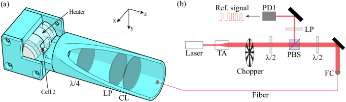
Figure S2: Schematic of the spin source. (a) Spin-source setup containing a ⁸⁷Rb vapor cell, a heater, and optical elements. A $5.8\,\text{cm}^{3}$ cubic vapor cell containing a droplet of ⁸⁷Rb and about 0.37 amg N₂ is heated to 180^∘C. The high-optical-power pump beam (0.5 W) is expanded and circularly polarized. ⁸⁷Rb spins are polarized to $\sim$92$\%$ and the number of polarized spins is calculated to be about $2.18\times 10^{14}$. (b) High-power pump system. An optical chopper modulates the laser beam with a square-wave pattern, with a frequency of about $10~{}\rm{Hz}$ and a duty cycle of about $50\%$, thus modulating the spin polarization of ⁸⁷Rb atoms. A half-wave plate and a polarizing beamsplitter are used to split the laser beam into two beams with different powers. The stronger one is coupled to a single-mode fiber with an optical fiber coupler. The weaker one is measured with PD1 to monitor the laser power. TA, tapered amplifier; $\lambda$/4, quarter-wave plate; $\lambda$/2, half-wave plate; CL, convex lens; PBS, polarizing beamsplitter; PD, photodiode; LP, linear polarizer; FC, fiber coupler.

As shown in Fig. S2(b), a high-power pump system containing a high-power pump laser of 795 nm (generated by a tapered amplifier laser system from TOPTICA Photonics Inc.) is used to polarize ⁸⁷Rb atoms in cell 2. In order to modulate the spin polarization of ⁸⁷Rb atoms, an optical chopper is placed in the laser path to periodically block the pump beam at a frequency $\nu\approx 10.00$ Hz with 50$\%$ duty cycle. Then a half-wave plate and a polarizing beamsplitter (PBS) are used to split the pump light into two beams with the power ratio of more than $100:1$. The weaker beam is monitored in real-time by a photodiode as reference signal and the stronger one is used for optical pumping. The second half-wave plate is used to adjust the light polarization of the laser beam for efficiently coupling the laser with a single-mode fiber. The coupling efficiency of the fiber is approximately $70\%$. The laser transmitted from the fiber is expanded by a beam expander and adjusted to be circularly polarized by a linear polarizer and a quarter-wave plate. These optical elements are placed in a cylinder box and are connected to the heating chamber, as shown in Fig. S2(a).

II.2 Calibration of spin-source parameters

The magnitude of the pseudomagnetic field generated by the spin source is proportional to the number of the polarized electron spins in the spin-source cell. Due to the optical absorption and spatial distribution of pump-beam intensity, the spin polarization is not uniform over the spin-source cell 2. Therefore, the pseudomagnetic field is dependent on the spatial spin distribution $\rho(\bm{r})$ in the spin source [see Eq. (S32)],

$$\rho(\bm{r})=n_{\rm{Rb}}\cdot P_{z}(\bm{r}),$$ (S11)

where $n_{\text{Rb}}$ is the number density of ⁸⁷Rb and $P_{z}(\bm{r})$ is the spin polarization of ⁸⁷Rb electrons at the position of $\bm{r}=(x,y,z)$. To obtain the spatial distribution of polarized electron spins, it is necessary to obtain the spatial distribution $\rho(\bm{r})$. In the following, we explain how to calibrate the key parameters $n_{\rm{Rb}}$ and $P_{z}(\bm{r})$.

1. Atomic absorption spectroscopy measurement

We use atomic absorption spectroscopy to calibrate the parameters of the optical pumping, such as the number density of ⁸⁷Rb atoms, collisionally shifted resonance frequency of D1 transition and the bandwidth caused by pressure broadening. A linearly polarized laser beam (the absorption-spectroscopy laser with small light power) with frequency tuned near the Rb D1 transition, propagating along $z$, travels through the spin-source cell 2. The absorption of such a linearly polarized laser is described by

$$I_{\rm{out}}=I_{\rm{in}}e^{-n_{\rm{Rb}}\sigma(\nu_{l})L},$$ (S12)

where $I_{\rm{out}}$ is the transmitted light intensity, $I_{\rm{in}}$ is the incident light intensity, $\sigma(\nu_{l})$ is the photon absorption cross-section, $\nu_{l}$ is the optical frequency of the absorption-spectroscopy laser, and $L$ is the length of spin-source cell 2. Due to the large pressure broadening by the buffer gas N₂, the absorption cross-section can be described as a function of the laser frequency $\nu_{l}$ with a Lorentzian lineshape [6]

$$\sigma(\nu_{l})=\pi r_{e}cf_{\rm{D1}}\frac{\Gamma/2\pi}{(\nu_{l}-\nu_{\text{D1}})^{2}+(\Gamma/2)^{2}},$$ (S13)

where $r_{e}$ is the classical radius of the electron, $c$ is the velocity of light, $f_{\rm{D1}}=1/3$ is the oscillator strength of the D1 transition, $\Gamma$ is the full-width at half-maximum (FWHM) of the lineshape mainly caused by N₂, and $\nu_{\text{D1}}$ is the collisionally shifted resonance frequency of D1 transition.

In the experiment, due to the unavoidable reflection from the vapor-cell glass and the window of the oven, the measured transmitted light intensity is reduced and described by $I^{\prime}_{\rm{out}}=\xi I_{\rm{out}}$. Based on Eqs. (S13) and (S12), optical absorption of the linearly polarized laser light can be written as

$$\ln{\frac{I^{\prime}_{\rm{out}}}{\xi I_{\rm{in}}}}=-\pi r_{e}cf_{\rm{D1}}n_{\rm{Rb}}L\frac{\Gamma/2\pi}{(\nu_{l}-\nu_{\text{D1}})^{2}+(\Gamma/2)^{2}}.$$ (S14)

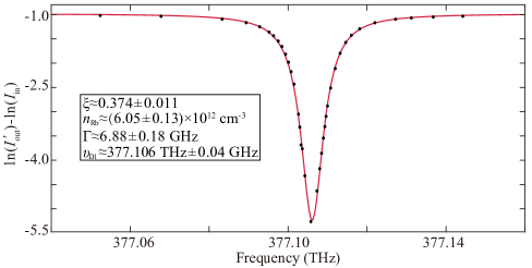
Figure S3: Rb atomic absorption spectrum at 100^∘C as an example. The parameters of the Lorentzian lineshape are fitted to $\xi\approx 0.374\pm 0.011$, $n_{\rm{Rb}}\approx(6.05\pm 0.13)\times 10^{12}~{}\rm{cm^{-3}}$, $\Gamma\approx 6.88\pm 0.18\,\rm{GHz}$ and $\nu_{\text{D1}}\approx 377.106\,\rm{THz}\pm 0.04\,\text{GHz}$. As the temperature rises, number density of ⁸⁷Rb increases and the corresponding optical absorption increases, rendering the transmitted light intensity near the resonance frequency hard to measure. Therefore, parameters independent of temperature, such as $\Gamma$ and $\nu_{\text{D1}}$, are determined at low temperature (100^∘C).

By detuning the laser frequency $\nu_{l}$, we measure the corresponding laser power of the incident light $I_{\rm{in}}$ and that of the transmitted light $I^{\prime}_{\rm{out}}$, and then obtain a profile. By fitting the profile, we obtain the key parameters $\xi$, $n_{\text{Rb}}$, $\Gamma$ and $\nu_{\text{D1}}$. We show an example of 100^∘C in Fig. S3, where $\xi$, $n_{\text{Rb}}$, $\Gamma$, and $\nu_{\text{D1}}$ are obtained. Using the same method for our final search experiment, we calibrate the ⁸⁷Rb number density as

$$n_{\text{Rb}}\approx(4.0\pm 0.2)\times 10^{14}~{}\text{cm}^{-3}.$$ (S15)

2. Calibration of the spin polarization

The spin polarization of ⁸⁷Rb electrons and its spatial distribution depend on the parameters of optical pumping. In the following, we determine the spin polarization based on calibrated optical-pumping parameters.

• Overview of the calibration method

  In our experiments, we use high-power circularly polarized laser light tuned near the Rb D1 transition to pump the spin-source cell 2. Due to the light absorption along $z$, the pumping rate and the corresponding spin polarization of Rb atoms are reduced along the light-propagation direction. The spin polarization can be generally expressed as

  $$P_{z}(\bm{r})=\frac{sR_{\text{OP}}(\bm{r})}{R_{\text{OP}}(\bm{r})+R_{\text{rel}}},$$ (S16)

  where $R_{\text{OP}}(\bm{r})$ is the pumping rate and $R_{\text{rel}}$ is the spin relaxation rate, $s=\pm 1$ is the photon spin component along the pumping direction. $s=-1$ corresponds to $\sigma^{-}$ light and $s=+1$ corresponds to $\sigma^{+}$ light. Here $R_{\text{OP}}(\bm{r})$ is position-dependent and $R_{\text{rel}}$ is position-independent.

  The spin-relaxation mechanisms include collisions with buffer-gas atoms, other alkali atoms and the wall of the vapor cell. In our experiments, by measuring the resonance linewidth at different pump powers, we determined the relaxation rate $R_{\rm{rel}}$ to be

  $$R_{\text{rel}}\approx 524\pm 18~{}\rm{s}^{-1}.$$ (S17)

  Because of the use of a strong laser ($\approx 0.5$ W) to pump cell 2, the pumping rate $R_{\text{OP}}(\bm{r})$ is much larger than the relaxation rate $R_{\text{rel}}$. As a result, the uncertainty of $R_{\text{rel}}$ contributes little to the uncertainty of the total number of polarized atoms as shown in Table S1.

  The pumping rate is the dominant factor influencing the polarization. Because the linewidth of the pump laser is much narrower than pressure-broadened linewidth of the atomic D1 transition ($\Gamma\approx 6.88\,$GHz), the incident pump light can be considered monochromatic. In this case, $R_{\text{OP}}$ is approximated as

  $$R_{\text{OP}}(\bm{r})\approx\sigma(\nu_{l})\cdot\Phi(\bm{r}),$$ (S18)

  where $\sigma(\nu_{l})$ is the photon-absorption cross-section of Rb D1 transition measured with atomic absorption spectroscopy [see Eq. (S13)], $\Phi(\bm{r})$ is the total flux of photons of frequency $\nu_{l}$ (in photons per unit area per unit time). $\Phi(\bm{r})$ can be expressed as a function of the intensity of the pump laser

  $$\Phi({\bm{r}})=I({\bm{r}})/h\nu_{l},$$ (S19)

  where $h\nu_{l}$ is the energy of an incident photon and $I({\bm{r}})$ is the light intensity. Due to the atomic absorption and cross-sectional shape of the incident light, $I({\bm{r}})$ depends on position. In the following, we analyse the spatial dependence of the incident light $I({\bm{r}})$.

• Distribution of the incident light intensity in the $xy$ plane

  The incident light is a Gaussian beam, whose light intensity is nonuniform in the $xy$ plane. Because the spin source (cell 2) is placed in the center of the beam, the distribution of the incident light intensity in the $xy$ plane can be written as (the direction and origin of the coordinate system are shown in the Fig. S4)

  $$I_{\text{in}}(x,y)=I(x,y,z=0)=\frac{2p}{\pi\omega^{2}}\text{exp}\left[-\frac{2(x^{2}+y^{2})}{\omega^{2}}\right],$$ (S20)

  where $p$ is the laser power and $\omega$ is the Gaussian beam waist radius. To obtain the spatial distribution of the incident light intensity, the incident light power $p$ and the spot radius of the expanded beam $\omega$ are required. The spot radius of the expanded beam is measured with a laser beam profiler (from Ophir-Spiricon Inc.),

  $$\omega\approx 2.99\pm 0.01~{}\rm{mm}.$$ (S21)

  The total power of the pump laser $p$ is measured at the position 1 (see Fig. S4) with an integrating sphere to be

  $$p\approx 0.50\pm 0.05\,\rm{W}.$$ (S22)

  Monitoring the laser power over a month, we find that the power variation does not exceed $10\%$ without any additional stabilization.

  

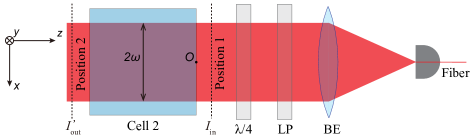
  Figure S4: Calibration of the incident light intensity in the $xy$ plane. By measuring the power $p$ and the beam waist radius $\omega$ of the pump laser at the position 1, we calibrate the distribution of the incident light intensity in the $xy$ plane. O, origin; BE, beam expander; LP, linear polarizer; $\lambda/4$, quarter-wave plate.

• Distribution of the light intensity along $z$

  On- or near-resonant light propagating through the vapor cell can be partially or completely absorbed by the alkali vapor. In order to obtain the distribution of the light intensity along $z$, we consider the attenuation of the circularly polarized light absorbed by the alkali metal atom

  $$\frac{\rm d}{\rm{d}z}I(\bm{r})=-n_{\rm{Rb}}\sigma(\nu_{l})I(\bm{r})\left[1-sP_{z}(\bm{r})\right].$$ (S23)

  Based on Eqs. (S16), (S18) and (S19), the differential equation (S23) can be reduced to that of one variable $I(\bm{r})$

  $$\frac{\rm d}{\rm{d}z}I(\bm{r})=-n_{\rm{Rb}}\sigma(\nu_{l})I(\bm{r})\left[1-\frac{\sigma(\nu_{l})I(\bm{r})}{\sigma(\nu_{l})I(\bm{r})+h\nu_{l}R_{\rm{rel}}}\right].$$ (S24)

  Equation (S24) at a fixed $(x,y)$ can be further simplified as [5]

  $$I(z)\cdot\text{exp}\left(\frac{\sigma(\nu_{l})I(z)}{h\nu_{l}R_{\text{rel}}}\right)=I_{\text{in}}\cdot\text{exp}\left[\frac{\sigma(\nu_{l})I_{\text{in}}}{h\nu_{l}R_{\rm{rel}}}-n_{\rm{Rb}}\sigma(\nu_{l})|z|\right].$$ (S25)

  To solve the above equation, we use the Lambert W-function, which is the inverse function of $f(W)=We^{W}$. Equation (S25) can be rewritten as the form of $We^{W}$

  $$\overbrace{\frac{\sigma(\nu_{l})I(z)}{h\nu_{l}R_{\text{rel}}}}^{W}\cdot\overbrace{\text{exp}\left(\frac{\sigma(\nu_{l})I(z)}{h\nu_{l}R_{\text{rel}}}\right)}^{e^{W}}=\overbrace{\frac{\sigma(\nu_{l})I_{\text{in}}}{h\nu_{l}R_{\text{rel}}}\cdot\text{exp}\left[\frac{\sigma(\nu_{l})I_{\text{in}}}{h\nu_{l}R_{\rm{rel}}}-n_{\rm{Rb}}\sigma(\nu_{l})|z|\right]}^{f(W)},$$ (S26)

  Using the Lambert W-function, we obtain

  $$I(z)=\frac{h\nu_{l}R_{\rm{rel}}}{\sigma(\nu_{l})}\cdot W\left[\frac{\sigma(\nu_{l})I_{\textrm{in}}}{h\nu_{l}R_{\rm{rel}}}\text{exp}\left(\frac{\sigma(\nu_{l})I_{\textrm{in}}}{h\nu_{l}R_{\rm{rel}}}-n_{\text{Rb}}\sigma(\nu_{l})|z|\right)\right].$$ (S27)

  This result is in a convenient form because $W$ is a known special function, built in software packages such as Mathematica^TM. Due to the optical absorption, the light intensity decreases as a function of $z$ as shown in Fig. S5(a).

  In order to maximize the average polarization of spin source, we should determine the optimal laser frequency. Figure S5(b) shows the average polarization versus the laser frequency detuning. The average polarization reaches a maximum when the frequency detuning is zero. Therefore, we adjust the laser frequency to the resonance frequency in our experiment. Using a wavelength meter to monitor the frequency for a month, the long-term frequency drift of the pump laser is measured to be

  $$\textrm{d}\nu_{l}\approx 0\pm 0.45~{}\rm{GHz}.$$ (S28)

  

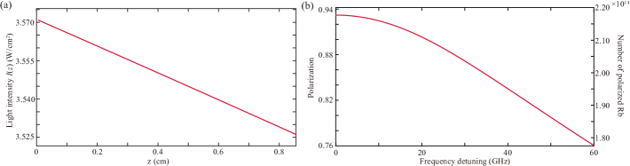
  Figure S5: (a) Variation curve of the light intensity of the spin-source pump laser along $z$ [see Eq. (S27)]. (b) Variation curve of average polarization with detuning. The total number of polarized atoms reaches maximum when the frequency detuning is 0. The vertical axis on the left represents the variation curve of average polarization with the frequency detuning.

Overall, with all the above parameters, we obtain the spin polarization at each position in the spin-source cell. The spatial polarization distribution of the spin source is shown in Fig. S6.

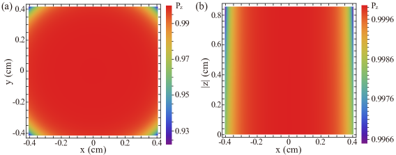
Figure S6: Spatial distribution of spin polarization in the spin source cell by numerical simulation. (a) Spatial polarization distribution in the $xy$ plane at $z=0$. (b) Spatial polarization distribution in the $xz$ plane at $y=0$.

II.3 Systematic errors of spin-source parameters

We first determine the mean value of the total number of polarized ⁸⁷Rb spins using the mean values of all experimental parameters. Based on the spatial distribution of the spin polarization, the total number of polarized ⁸⁷Rb electron spins is obtained by integrating over the spin-source cell $N=\int_{V}\rho(\bm{r})\rm{d}\bm{r}$. Subsequently, we obtain the error of the number of polarized ⁸⁷Rb by determining and combining the systematic errors of all experimental parameters (see Table S1). Here, we take the laser power $p$ as an example to show how to derive the systematic error of the number of polarized ⁸⁷Rb caused by the fluctuation of laser power. The number density of polarized ⁸⁷Rb $\rho(\bm{r})$ is re-estimated with the upper/lower limit of the pump power and mean values of other experimental parameters ( see Eq. S11 and Sec. II.2). Then, the number of polarized ⁸⁷Rb is obtained by integrating over the spin-source cell 2. The upper (lower) limit $N^{+}$ ($N^{-}$) on the number of polarized ⁸⁷Rb is calculated by using the upper (lower) limit of the pump power $0.55\,\rm W$ ($0.45\,\rm W$), i.e., $\Delta N^{\pm}=|N^{\pm}-N_{0}|\approx 0.02\times 10^{14}$, where $N_{0}$ is the number of polarized ⁸⁷Rb with the mean value of the pump power (0.5 W). The systematic errors caused by other parameters in Table S1 are determined by using the same procedure. The overall systematic error $\pm 0.18\times 10^{14}$ is derived by combining all the systematic errors in quadrature. The total number of polarized ⁸⁷Rb is $N\approx(2.18\pm 0.18)\times 10^{14}$.

Table S1:    Summary of experimental parameters and systematic error sources for the number of polarized Rb atoms.

Parameter	Value	$\Delta N\left(\times 10^{14}\right)$
Length of spin source $L$ (mm)	$8.6\pm 0.05$	$\pm 0.02$
Width of spin source $W$ (mm)	$8.1\pm 0.01$	$\pm 0.03$
Height of spin source $H$ (mm)	$8.3\pm 0.02$	$\pm 0.12$
Number density of rubidium $n_{\text{Rb}}$ (cm-3)	$(4.0\pm 0.2)\times 10^{14}$	${}^{+0.12}_{-0.11}$
Full-width at half-maximum $\Gamma$ (GHz)	$6.88\pm 0.30$	$<0.01$
Relaxation rate $R_{\text{rel}}$ ($s^{-1}$)	$524\pm 18$	$\pm 0.01$
Beam waist $\omega$ ($\rm{mm}$)	$2.99\pm 0.01$	${}^{+0.02}_{-0.03}$
Laser power $p$ (W)	$0.50\pm 0.05$	$\pm 0.02$
Frequency detuning $\textrm{d}\nu_{l}$ (GHz)	$0\pm 0.45$	$<0.01$
Total Num of polarized rubidium $N$ $(\times 10^{14})$	$2.18$	$\pm 0.18$

III Numerical simulation of the exotic pseudomagnetic field

Based on the number density of polarized ⁸⁷Rb spins $\rho(\textbf{r})$ obtained in the previous section, this section presents the numerical calculation of the pseudomagnetic field generated by the exotic interaction $V_{pp}$, including the field strength and direction. The spin-dependent interaction studied here is [3, 4]

$$V_{pp}=-\frac{g_{p}^{e}g_{p}^{n}}{16\pi m_{1}m_{2}}\left[(\hat{\bm{\sigma}}_{1}\cdot\hat{\bm{\sigma}}_{2})\left(\frac{m_{a}}{r^{2}}+\frac{1}{r^{3}}\right)-(\hat{\bm{\sigma}}_{1}\cdot\hat{\bm{r}})(\hat{\bm{\sigma}}_{2}\cdot\hat{\bm{r}})\left(\frac{m_{a}^{2}}{r}+\frac{3m_{a}}{r^{2}}+\frac{3}{r^{3}}\right)\right]e^{-m_{a}r},$$ (S29)

where $g_{p}^{e}g_{p}^{n}$ is the product of electron and neutron pseudoscalar coupling constants for $V_{pp}$, $\hat{\bm{\sigma}}_{i}$ is the spin vector of $i$th fermion and $m_{i}$ is its mass, $r$ is the distance between the two interacting fermions, $\hat{\bm{r}}$ is the corresponding unit vector, and $m_{a}$ is the axion mass.

The exotic interaction $V_{pp}$ can induce energy shift of ¹²⁹Xe spins in the spin sensor

$$-\mu_{\rm{Xe}}\bm{\hat{\sigma}}_{i}\cdot\bm{B}_{a}^{*}=V_{pp},$$ (S30)

where $\mu_{\text{Xe}}$ is the magnetic moment of ¹²⁹Xe spin. According to the Eqs. (S29) and (S30), the pseudomagnetic field $\bm{B}^{*}_{a}$ generated by a single electron spin is

$$\bm{B}^{*}_{a}=\frac{g_{p}^{e}g_{p}^{n}}{16\pi\mu_{\text{Xe}}m_{1}m_{2}}\left[\hat{\bm{\sigma}}_{2}\left(\frac{m_{a}}{r^{2}}+\frac{1}{r^{3}}\right)-\hat{\bm{r}}(\hat{\bm{\sigma}}_{2}\cdot\hat{\bm{r}})\left(\frac{m_{a}^{2}}{r}+\frac{3m_{a}}{r^{2}}+\frac{3}{r^{3}}\right)\right]e^{-m_{a}r}.$$ (S31)

With respect to all polarized electron spins and their spatial distribution in the spin source, the total pseudomagnetic field generated is

$$\bm{B}_{a} =\int_{V}\rho(\bm{r})\bm{B}^{*}_{a}(\bm{r})\rm{d}\bm{r}$$

$$=\frac{g_{p}^{e}g_{p}^{n}}{16\pi\mu_{\text{Xe}}m_{1}m_{2}}\int_{V}\rho(\bm{r})\left[\hat{\bm{\sigma}}_{2}\left(\frac{m_{a}}{r^{2}}+\frac{1}{r^{3}}\right)-\hat{\bm{r}}(\hat{\bm{\sigma}}_{2}\cdot\hat{\bm{r}})\left(\frac{m_{a}^{2}}{r}+\frac{3m_{a}}{r^{2}}+\frac{3}{r^{3}}\right)\right]e^{-m_{a}r}\rm{d}\bm{r},$$ (S32)

where $V$ is the volume of spin source, $\rho(\bm{r})$ is the number density of polarized spins at the position $\bm{r}$ in the spin source. According to the position of spin source and the direction polarized electron spins, as shown in the Fig. 1 of the main text, $\bm{B}_{a}$ can be rewritten to

$$\bm{B}_{a}=B^{y}_{a}\hat{\bm{y}}+B^{z}_{a}\hat{\bm{z}}.$$ (S33)

Because the spin-based amplifier is insensitive to the pseudomagnetic field along $z$, $B^{z}_{a}\hat{\bm{z}}$ is negligible and $B^{y}_{a}\hat{\bm{y}}$ is considered.

To generate the resonant pseudomagnetic field (an osillating field), we use an optical chopper with 50$\%$ duty cycle to periodically block the pump light at the frequency of $\nu\approx 10.00$ Hz. Because the ⁸⁷Rb electron relaxation time ($\sim 1$ ms) is much shorter than the modulation period ($\sim 100$ ms), the modulated electron polarization can be thought of as changing instantaneously. Based on the variation of light intensity with time detected by PD1, we take $g_{p}^{e}g_{p}^{n}/4=1$ and $m_{a}=0.1~{}$meV as an example to present the field strength and waveform of the pseudomagnetic field signal, as shown in Fig. S7(a). Furthermore, the frequency spectrum of the pseudomagnetic field signal can be obtained by performing discrete Fourier transform of the time domain signal. As shown in Fig. S7(b), the square wave signal $B^{y}_{a}$ contains trigonometric function signals with harmonic frequencies at $\nu$, 3$\nu$, 5$\nu$,… and the pseudomagnetic field along $y$ can be decomposed into

$$B^{y}_{a}=\sum\limits_{N=\text{odd}}B^{(N)}_{\text{ac}}\cos(2\pi N\nu t+\phi^{(N)}_{0}),$$ (S34)

where $\phi^{(N)}_{0}$ and $B^{(N)}_{\text{ac}}$ is the phase and the strength of the $N$th harmonic field. The ratios of the strengths are calculated to be $B_{\text{ac}}^{(1)}:B_{\text{ac}}^{(3)}:B_{\text{ac}}^{(5)}\approx 13.0:4.3:2.5$. In experiment, we can only detect one harmonic because of the narrow bandwidth $\approx$ 49 mHz. Therefore, we choose to detect the first harmonic $B_{\text{ac}}^{(1)}$ by tuning the resonant frequency $\nu_{0}$ of spin-based amplifier to 10.00 Hz.

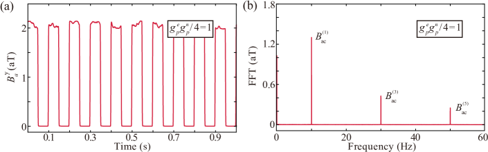
Figure S7: Simulations of $V_{pp}$ produced by the spin source. Assuming $g_{p}^{e}g_{p}^{n}/4=1$ and $m_{a}=0.1~{}$meV, the signal of the simulated pseudomagnetic field $\bm{B}_{a}$ generated by the spin source is obtained. (a) Time-domain signal of $B^{y}_{a}$. (b) Fourier transformation spectrum of $B^{y}_{a}$.

IV Dipole magnetic field generated by the spin source

In this section, we theoretically calculate and experimentally measure the dipole magnetic field generated by the polarized ⁸⁷Rb atoms in the spin source without magnetic shields. If not properly shielded, the classical magnetic field is a spurious signal. In the following, we discuss how to measure and remove the undesired field.

IV.1 Numerical calculation of the dipole magnetic field

The dipole magnetic field generated by a single polarized ⁸⁷Rb atom at position $\bm{r}$ can be expressed as

$$\bm{B}^{*}_{d}=\frac{\mu_{0}}{4\pi}\frac{3\hat{\bm{r}}(\hat{\bm{r}}\cdot\bm{\mu}_{e})-\bm{\mu}_{e}}{r^{3}}=\frac{\mu_{0}\mu_{e}}{4\pi}\frac{3\hat{\bm{r}}(\hat{\bm{r}}\cdot\hat{\bm{\sigma}}_{2})-\hat{\bm{\sigma}}_{2}}{r^{3}},$$ (S35)

where $\mu_{0}$ is the vacuum permeability, $\hat{\bm{r}}$ is the unit vector of position vector $\bm{r}$, $\mu_{e}$ is the magnetic dipole moment of the electron spin, and $\hat{\bm{\sigma}}_{2}$ is its spin vector. Combining with the number density and direction of polarized ⁸⁷Rb spins in the spin source, the strength and direction of the dipole magnetic field generated by the spin source can be calculated as

$$\bm{B}_{d} =\int_{V}\rho(\bm{r})\bm{B}^{*}_{d}(\bm{r})\rm{d}\bm{r}$$

$$=\frac{\mu_{0}\mu_{e}}{4\pi}\int_{V}\rho(\bm{r})\left[\frac{3\hat{\bm{r}}(\hat{\bm{r}}\cdot\hat{\bm{\sigma}}_{2})-\hat{\bm{\sigma}}_{2}}{r^{3}}\right]\rm{d}\bm{r},$$ (S36)

where $V$ represents the integration space in the internal volume of the spin-source cell 2, $\rho(\bm{r})$ is the number density of polarized spins at the position $\bm{r}$. The dipole field at the center of the spin-based amplifier is $\bm{B}_{d}=B_{d}^{x}\hat{\bm{x}}+B_{d}^{y}\hat{\bm{y}}+B_{d}^{z}\hat{\bm{z}}$ with three components

$$B^{x}_{d} =0.3~{}\textrm{pT},$$ (S37)

$$B^{y}_{d} =-3.1~{}\textrm{pT},$$

$$B^{z}_{d} =2.8~{}\textrm{pT}.$$

IV.2 Calibration of the dipole magnetic field

In order to accurately calibrate the strength of the dipole magnetic field, we use a commercial miniature rubidium magnetometer (from QuSpin Inc.), which is a centimeter-scale spin-exchange-relaxation-free (SERF) magnetometer. This measurement is performed without small-size magnetic shields for the spin sensor and spin source (see Fig. S9). The magnetic-field sensitivity is about 20 fT/Hz^1/2 at frequencies ranging from 3 to 100 Hz. In order to measure the dipole field at the spin sensor, we first remove the spin sensor and place the QuSpin magnetometer at the same position and then modulate the dipole field with an optical chopper that periodically blocks the high-power pump beam at a frequency $\nu\approx 10.00$ Hz (see Sec. II). As shown in Fig. S8, there is a notable peak at about 10.00 Hz and the dipole magnetic field is measured to be about 3.22 pT, in good agreement with the finite element analysis of magnetic field [see Eq. (S37)].

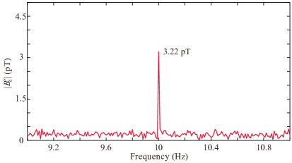
Figure S8: Classical magnetic dipole field measured with a commercial miniature magnetometer without magnetic shields. A frequency spectrum of the time-domain signal acquired with a QuSpin magnetometer. A dipole field $\approx 3.22$ pT is measured

IV.3 Experimental elimination of the dipole magnetic field

It is important to eliminate the dipole magnetic field that would generate the spurious signal hard to distinguish from the exotic interaction. To do this, we design and use small-size mu-metal shields for the spin sensor and spin source. As shown in Fig. S9, the spin sensor (cell 1) is magnetically shielded with a single layer of 1 mm thickness mu-metal shield, inside which a set of Helmholtz coils is used to provide bias magnetic field. The spin source (cell 2) is magnetically shielded with two layers of 0.5 mm thickness mu-metal shields, where the gap between the two layers is filled with aerogel for thermal insulation.

The shielding factor of mu-metal shields is calibrated with a fluxgate magnetometer. The 1 mm single-layer mu-metal shield for the spin sensor has a shielding factor of about $100$, and the shielding factor of the two-layer shield for the spin source is about $4\times 10^{4}$. As a result, the total shielding factor is more than $10^{6}$. The strength of the dipole magnetic field generated on the spin sensor should be less than $3\,\textrm{aT}$, which is much less than the 24-hour magnetic-field detection limit of the spin sensor (76 aT). Therefore, the remaining magnetic dipole field can be neglected after adding the shields.

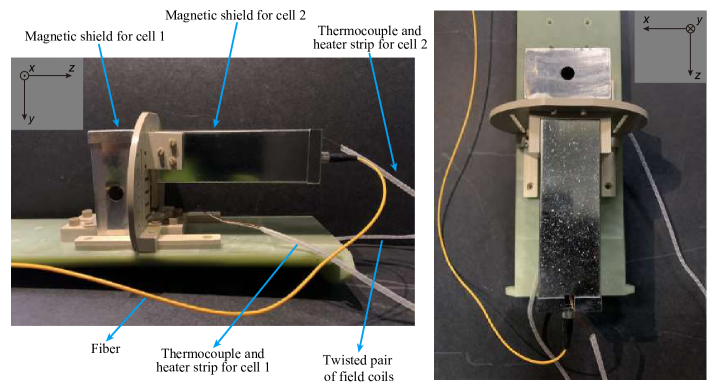
Figure S9: Magnetic shields for eliminating the dipole magnetic field. Both of the spin sensor (cell 1) and the spin source (cell 2) are shielded with mu-metal magnetic shields.

V Data analysis

This section presents the procedure to determine the constraint on $g_{p}^{e}g_{p}^{n}$ and the data analysis of exotic-interaction-search experiments. The procedure includes five parts: the calibration experiment, the search experiment, analysis of mean values and statistical errors, analysis of systematic errors and, finally, the extraction of the constraint.

Table S2:    Summary of corrections to $|g_{p}^{e}g_{p}^{n}|/4$ (presented here for $m_{a}=0.1$ meV) and systematic errors.

Parameter	Value	$\Delta g_{p}^{e}g_{p}^{n}/4$
Position of cell 2 $x$ (mm)	$1.9\pm 0.2$	${}^{<0.01}_{-0.04}$
Position of cell 2 $y$ (mm)	$-23.1\pm 1.0$	${}^{-0.98}_{+1.23}$
Position of cell 2 $z$ (mm)	$41.9\pm 0.3$	${}^{+0.75}_{-0.69}$
Num. of polarized Rb ($10^{14}$)	$2.18\pm 0.18$	${}^{-0.41}_{+0.44}$
Phase delay $\phi$ (deg)	$102.6\pm 0.6$	${}^{-1.45}_{+1.45}$
Calib. const. $\alpha$ (V/nT)	$2.11^{+0.002}_{-0.386}$	${}^{-0.01}_{+1.20}$
Final $|g_{p}^{e}g_{p}^{n}|/4$	$5.3$	$\pm 48.5\ (\text{statistical})$
$(m_{a}=0.1~{}\text{meV})$		$\pm 2.4\ (\text{systematic})$

V.1 Calibration experiment

To analyze the strength and phase of the pseudomagnetic field signal from $V_{pp}$, we calibrate experimental parameters in advance, including the position of the spin source $\bm{r}$, number density of polarized spins in the spin source $\rho(\bm{r})$, phase delay $\phi$ and calibration constant $\alpha$ of the spin-based amplifier, etc. With the position $\bm{r}$ and the number density of polarized spins $\rho(\bm{r})$, the magnitude of the pseudomagnetic field generated by the spin source can be calculated according to Eq. (S32). In addition, the phase delay $\phi$ and calibration constant $\alpha$ are used to determine the amplitude and phase of the output-voltage signal generated by the pseudomagnetic field. Table S2 shows the mean values and uncertainties of the physical parameters above. In the following, we explain the details of such parameters.

• Calibration of the position of spin source. We measure the position of the spin source $\bm{r}=(x,y,z)$. The coordinate axis directions are shown in Fig. S1. The position of the center of the spin source (cell 2) relative to the origin of coordinate (the center point of the cell 1) is

  $$x \approx 1.9\pm 0.2~{}\textrm{mm},$$ (S38)

  $$y \approx-23.1\pm 1.0~{}\textrm{mm},$$

  $$z \approx 41.9\pm 0.3~{}\textrm{mm}.$$

  The length, width and height of the spin source are shown in Table S1. According to the center position $\bm{r}$ and size of the spin source, the position of a single micro-element relative to the origin is determined and further used to determine the number density of polarized ⁸⁷Rb atoms for this micro-element.

• Calibration of number density of polarized spins in the spin source. In order to calculate the amplitude of the pseudomagnetic field generated by the spin source, we need to calibrate the number density of polarized ⁸⁷Rb atoms at each position in the spin source $\rho(\bm{r})=n_{\text{Rb}}\cdot P_{z}(\bm{r})$ [see Eq. (S32)]. The calibration procedure is described in Sec. II.2 and we only present the result here. The total number of polarized ⁸⁷Rb atoms in the spin source is calculated based on $N=\int_{V}\rho(\bm{r})\text{d}\bm{r}$ and presented in Table S1

  $$N\approx(2.18\pm 0.18)\times 10^{14}.$$ (S39)

• Determination of the calibration constant $\alpha$. The calibration constant $\alpha$ (V/nT) of the spin-based amplifier describes the conversion coefficient between the strength of input magnetic field and the output voltage signal of the spin-based amplifier. To measure $\alpha$, we apply a known oscillating magnetic field along $y$ and measure the amplitude of the output-voltage signal. The calibration constant $\alpha$ is determined as

  $$\alpha\approx 2.11^{+0.002}_{-0.386}~{}\textrm{V/nT}.$$ (S40)

  The uncertainty of the calibration constant $\alpha$ is determined by two aspects:

• The intrinsic instability of the spin-based amplifier $\delta\alpha_{\textrm{int}}$. The intrinsic instability $\delta\alpha_{\textrm{int}}$ can be caused by technical sources of random fluctuations, such as the bias magnetic field along $z$, variations in vapor-cell temperature and optical power, etc. To calibrate $\delta\alpha_{\textrm{int}}$, we measure the output signal of the spin-based amplifier for one hour with an oscillating magnetic field applied. According to the fluctuation of the output signal strength, we obtain the intrinsic instability $\delta\alpha_{\textrm{int}}\approx\pm 0.002~{}\textrm{V/nT}$.

• The external instability of input-signal frequency $\delta\alpha_{\textrm{ext}}$ from the instability of the chopper. The instability of pseudomagnetic field frequency $\delta\nu$ is caused by the fluctuation of chopper frequency, which is calibrated as $\delta\nu\approx\pm 10~{}\textrm{mHz}$ by monitoring the frequency stability of output chopper signal at PD2 for a long time. The mismatch between the input-signal frequency and the resonance frequency of the spin-based amplifier would weaken the amplification effect. The calibration constant $\alpha(\nu)$ can be described by the lineshape formula

  $$\alpha(\nu)=\alpha(\nu_{0})\dfrac{\Lambda/2}{\sqrt{(\nu-\nu_{0})^{2}+(\Lambda/2)^{2}}},$$ (S41)

  where $\Lambda\approx 28~{}\textrm{mHz}$. Assuming $(\nu-\nu_{0})\approx\delta\nu$ in Eq. (S41), the external uncertainty can be $\delta\alpha_{\textrm{ext}}\approx-0.386~{}\textrm{V/nT}$. Combining $\delta\alpha_{\textrm{int}}$ and $\delta\alpha_{\textrm{ext}}$, the total uncertainty $\delta\alpha$ of the spin-based amplifier is determined as $\alpha\approx 2.11^{+0.002}_{-0.386}~{}\textrm{V/nT}$.

• Calibration of the phase delay $\phi$. The phase delay of the spin-based amplifier $\phi$ denotes the phase difference between the input-magnetic-field signal and the output-voltage signal of the spin-based amplifier. In the actual measurement process, we apply an oscillating magnetic field along $y$ with known phase $\phi_{0}$ and frequency $\nu$. Then, the phase delay of the spin-based amplifier is obtained by measuring the difference between the phase of the output voltage signal and the phase of the input magnetic field. The phase delay is determined as

  $$\phi\approx 102.6\pm 0.6~{}\textrm{deg},$$ (S42)

  where the uncertainty of phase delay $\phi$ is obtained by repeating the above process and calculating the corresponding variance.

The experimental parameters determined in the calibration experiments are listed in the second column of Table S2. Using the calibration constant $\alpha$ and the phase delay $\phi$ of the spin-based amplifier, the output voltage signal of the spin-based amplifier can be determined as $\alpha B^{y}_{ac}\cos(2\pi\nu t+\phi_{0}-\phi)$. Then, the pseudomagnetic field can be obtained from the experimental data as discussed in Sec. V.3 and V.4 .

V.2 Search experiment

Throughout the experiment, the spin-based amplifier is tuned to match the optical chopping frequency of the spin-source pump laser, i.e., $\nu_{0}\approx\nu\approx 10.00$ Hz. Due to the narrow bandwidth (49 mHz) of the amplifier, only the first harmonic of the pseudomagnetic field can be amplified and the effect of other harmonics is negligible (see Sec. III). The data were collected in six-hour batches, after which the spin-based amplifier was readjusted to optimize the magnetic-field sensitivity by tweaking the bias field, etc. (see Sec. I). While recording search data, the parameters of the spin source were monitored, such as the chopper frequency and pump power. The total duration of the search experiment was about 24 h.

V.3 Analysis of mean values and statistical errors

We now describe how to obtain the constraints on the product of coupling constants $|g_{p}^{e}g_{p}^{n}|/4$ from the experimental search data. A “lock-in” detection scheme is used to extract the weak signal from the pseudomagnetic fields with a known carrier frequency from noisy signal [2, 7]. The procedure is divided into two steps.

• Step 1: Obtain the product of coupling constants $g_{p}^{e}g_{p}^{n}/4$ for one-hour batches.

• After applying a band-pass filter around the resonance frequency on the data, the noise such as power-frequency noise (50 Hz, 100 Hz, …) can be filtered out. The filtered time-domain data are further separated into segments of one period $S(t)^{i}$.

• The normalized reference signal $\cos{(2\pi\nu t+\phi_{0}^{(1)}-\phi)}$ of every individual period is simulated based on Eq. (S34), corresponding to $g_{p}^{e}g_{p}^{n}/4=1$ for the mass $m_{a}=0.1$ meV based on experimental parameters in Table S2.

• Using “lock-in” detection scheme, we extract every product of coupling constants $g_{p}^{e}g_{p}^{n}/4$ for every period $S(t)^{i}$ ($T\approx 100$ ms)

  $$(g_{p}^{e}g_{p}^{n})^{i}/4=\frac{1}{\alpha B^{(1)}_{\textrm{ac}}}\frac{\int^{T}_{0}\cos{(2\pi\nu t+\phi_{0}^{(1)}-\phi)}S(t)^{i}\textrm{d}t}{\int^{T}_{0}\cos^{2}{(2\pi\nu t+\phi_{0}^{(1)}-\phi)}\textrm{d}t},$$ (S43)

  where $B^{(1)}_{\textrm{ac}}$ is the first harmonic corresponding to $g_{p}^{e}g_{p}^{n}/4=1$ (see Sec. III). Figure S10 shows the graph of all products of coupling constants $g_{p}^{e}g_{p}^{n}/4$ obtained for the-first-hour batches. The fit with Gaussian distribution to the histogram gives the mean value and the standard error of the products of coupling constants $g_{p}^{e}g_{p}^{n}/4$,

  $$(g_{p}^{e}g_{p}^{n})^{\textrm{1~{}h}}/4\approx 52.7\pm 218.0_{\textrm{stat}},$$ (S44)

  where the superscript 1 h represents first one-hour batch. By repeating the above three steps, 24 products of coupling constants $g_{p}^{e}g_{p}^{n}/4$ are obtained.

  

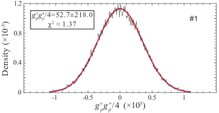
  Figure S10: The graph of the potential experimental coupling strength $(g_{p}^{e}g_{p}^{n})^{\text{1~{}h}}/4$. Distribution of the experimental coupling strength $(g_{p}^{e}g_{p}^{n})^{\textrm{1~{}h}}/4$ of the-first-hour data. The red solid line is a fit to a Gaussian distribution. The average and the standard error of the coupling strength is $(g_{p}^{e}g_{p}^{n})^{\textrm{1~{}h}}/4\approx 52.7\pm 218.0$. The $\chi^{2}\approx 1.37$ represents a valid fitting.

• Step 2: We use the reduced $\chi^{2}$ statistic to obtain the mean value and standard error of the products of coupling constants $(g_{p}^{e}g_{p}^{n})/4$ for 24-hour batches. The weighted average and the standard error of the product of coupling constants $|g_{p}^{e}g_{p}^{n}|/4$ is defined as [8]

  $$\left<x\right>=\left|\frac{\Sigma^{N}_{i=1}\varpi^{i}x^{i}}{\Sigma^{N}_{i=1}\varpi^{i}}\right|,$$ (S45)

  $$\Delta x=\frac{1}{\sqrt{\Sigma^{N}_{i=1}\varpi^{i}}},$$

  where $x$ represents $|g_{p}^{e}g_{p}^{n}|/4$, $x^{i}\pm\sigma^{i}$ is the mean value and the standard error of coupling constants $|g_{p}^{e}g_{p}^{n}|^{i}/4$ for one hour, the weights are defined as $\varpi^{i}=\left(1/\sigma^{i}\right)^{2}$. The values with the smaller $\sigma^{i}$ carry the larger statistical weight. The weighted reduced $\chi^{2}$ is

  $$\chi^{2}=\frac{\Sigma^{N}_{i=1}\varpi^{i}}{(\Sigma^{N}_{i=1}\varpi^{i})^{2}-\Sigma^{N}_{i=1}(\varpi^{i})^{2}}\cdot\sum_{i=1}^{N}\frac{\varpi^{i}(x^{i}-\left<x\right>)^{2}}{(\sigma^{i})^{2}}.$$ (S46)

  Based on the $\chi^{2}$ statistic, the mean value and standard error of the products of coupling constants $|g_{p}^{e}g_{p}^{n}|/4$ for 24-hour batches is $5.3\pm 48.5_{\rm{stat}}$ and the weighted reduced $\chi^{2}$ is $1.65$.

V.4 Analysis of systematic errors

As was shown above, the mean value and the standard error of the parameters are obtained. Then we can determine the mean value and statistical errors of the coupling strength (the product of coupling constants $|g_{p}^{e}g_{p}^{n}|/4$). This section analyzes the error of the coupling strength caused by the systematic errors of experimental parameters (see Table S2).

Consider the example of calibration constant $\alpha$, we determine its systematic error using three steps shown in Fig. S11:

• Obtaining the reference signal. By substituting the upper limit of the calibration constant $\alpha=2.110+0.002~{}\textrm{V/nT}$ and the mean values of other parameters (see Table S2) into Eq. (S43), we obtain the reference signal corresponding to the upper limit of the calibration constant.

• Extracting the coupling strength. By using the reference signal obtained above, we can extract the corresponding coupling strength $(|g_{p}^{e}g_{p}^{n}|/4)^{i+}$ by employing the “lock-in” detection scheme.

• Determine the systematic error. The systematic error caused by the upper limit of the calibration constant is determined by the difference $\Delta(|g_{p}^{e}g_{p}^{n}|/4)^{i+}=(|g_{p}^{e}g_{p}^{n}|/4)^{i+}-|g_{p}^{e}g_{p}^{n}|/4\approx-0.01.$ Similarly, we can obtain the systematic error corresponding to the lower limit of the calibration constant $\alpha=2.110-0.386~{}\textrm{V/nT}$, which is given by $\Delta(|g_{p}^{e}g_{p}^{n}|/4)^{i-}=(|g_{p}^{e}g_{p}^{n}|/4)^{i-}-|g_{p}^{e}g_{p}^{n}|/4\approx+1.20$.

Based on these procedures, the systematic errors caused by other calibration parameters in Table S2 are determined. Finally, we can derive the overall systematic error $\pm 2.4_{\textrm{sys}}$ by combining all the systematic errors in quadrature, and the final coupling strength is

$$|g_{p}^{e}g_{p}^{n}|/4\approx 5.3\pm 48.5_{\textrm{stat}}\pm 2.4_{\textrm{sys}}.$$ (S47)

.

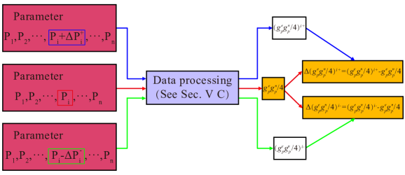
Figure S11: Procedures for determining systematic errors. The left part represents the average value and standard error of parameters. The middle part represents the data processing (see Sec. V.3). The right part represents the determined systematic errors.

V.5 Extraction of the constraint

Based on the above data analysis, the constraint on coupling strength at a specific mass $m_{a}$ is determined. Taking $m_{a}=0.1~{}\textrm{meV}$ as an example, the constraints on $|g_{p}^{e}g_{p}^{n}|/4$ at confidence level of 95$\%$ (corresponding to 1.96$\sigma$) can be determined as

$$5.3+1.96\times\sqrt{48.5^{2}_{\textrm{stat}}+2.4^{2}_{\textrm{sys}}}\approx 100.$$ (S48)

Further, by repeating the data analysis in Secs. V.3 and V.4 and changing mass $m_{a}$, the constraints for the entire explored mass range are obtained, as shown in Fig. 4 in the main text. Finally, we establish the constraints on the exotic spin-spin interaction between polarized electron and neutron spins in the axion window (1$~{}\mu$eV-1 meV), which corresponds to a force range from 0.2 mm to 20 cm. In particular, we obtain the most stringent constraints on $|g_{p}^{e}g_{p}^{n}|/4$ for the mass range from 0.03 meV to 1 meV.

References

- [1] Jiang, M., Su, H., Garcon, A., Peng, X. & Budker, D. Search for axion-like dark matter with spin-based amplifiers. Nat. Phys. 17, 1402–1407 (2021).
- [2] Su, H. et al. Search for exotic spin-dependent interactions with a spin-based amplifier. Sci. Adv. 7, eabi9535 (2021).
- [3] Fadeev, P. et al. Revisiting spin-dependent forces mediated by new bosons: Potentials in the coordinate-space representation for macroscopic-and atomic-scale experiments. Phys. Rev. A 99, 022113 (2019).
- [4] Dobrescu, B. A. & Mocioiu, I. Spin-dependent macroscopic forces from new particle exchange. J. High Energy Phys. 2006, 005 (2006).
- [5] Walker, T. G. & Happer, W. Spin-exchange optical pumping of noble-gas nuclei. Rev. Mod. Phys. 69, 629 (1997).
- [6] Romalis, M. V., Miron, E. & Cates, G. D. Pressure broadening of rb and lines by , , , and Xe: Line cores and near wings. Phys. Rev. A 56, 4569–4578 (1997).
- [7] Ji, W. et al. New experimental limits on exotic spin-spin-velocity-dependent interactions by using SmCo5 spin sources. Phys. Rev. Lett. 121, 261803 (2018).
- [8] Lee, J., Almasi, A. & Romalis, M. Improved limits on spin-mass interactions. Phys. Rev. Lett. 120, 161801 (2018).