Ranking Info Noise Contrastive Estimation: Boosting Contrastive Learning via Ranked Positives

Abstract

This paper introduces Ranking Info Noise Contrastive Estimation (RINCE), a new member in the family of InfoNCE losses that preserves a ranked ordering of positive samples. In contrast to the standard InfoNCE loss, which requires a strict binary separation of the training pairs into similar and dissimilar samples, RINCE can exploit information about a similarity ranking for learning a corresponding embedding space. We show that the proposed loss function learns favorable embeddings compared to the standard InfoNCE whenever at least noisy ranking information can be obtained or when the definition of positives and negatives is blurry. We demonstrate this for a supervised classification task with additional superclass labels and noisy similarity scores. Furthermore, we show that RINCE can also be applied to unsupervised training with experiments on unsupervised representation learning from videos. In particular, the embedding yields higher classification accuracy, retrieval rates and performs better in out-of-distribution detection than the standard InfoNCE loss.

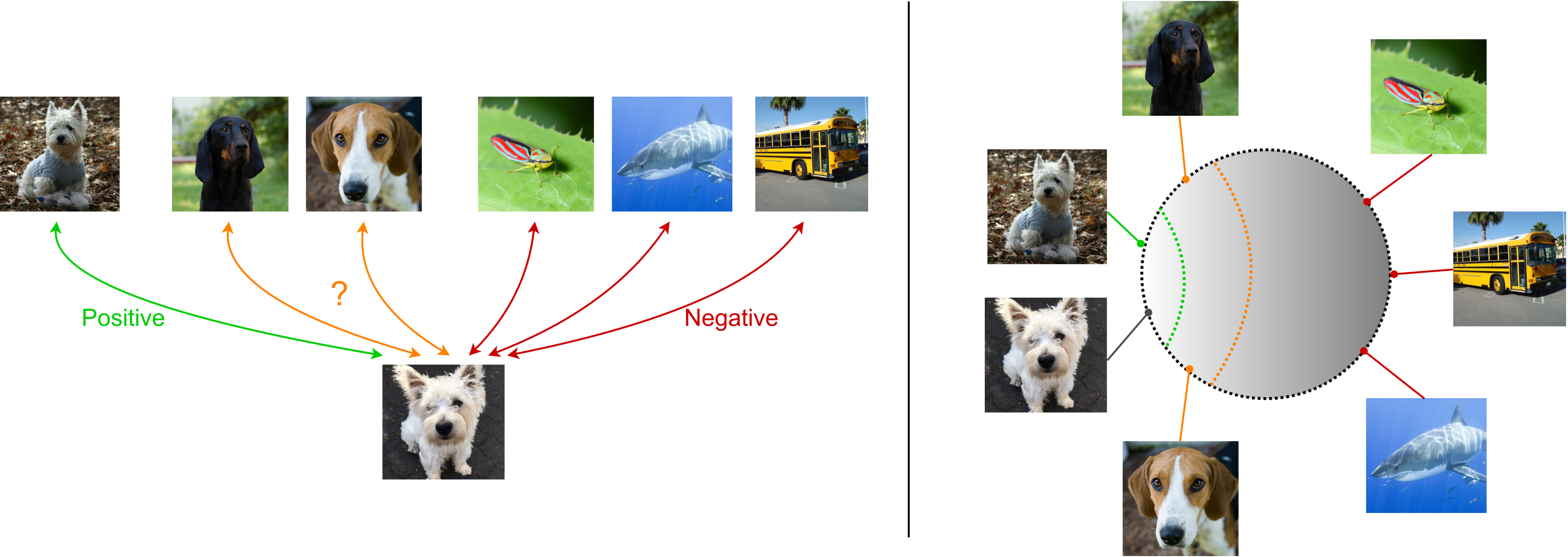
Figure 1: Contrastive Learning should not be binary. In many scenarios a strict separation of samples in “positives” and “negatives” is not possible. So far, this grey zone (left) was neglected, leading to sub-optimal results. We propose a solution to this problem, which embeds same samples very close and similar samples close in the embedding space (right).

Introduction

Contrastive learning recently triggered progress in self-supervised representation learning. Most existing variants require a strict definition of positive and negative pairs used in the InfoNCE loss or simply ignore samples that can not be clearly classified as either one or the other (Zhao et al. 2021). Contrastive learning forces the network to impose a similar structure in the feature space by pulling the positive pairs closer to each other while keeping the negatives apart.

This binary separation into positives and negatives can be limiting whenever the boundary between those is blurry. For example, different samples from the same classes are used as negatives for instance recognition, which prevents the network from exploiting their similarities. One way to address this issue is supervised contrastive learning (SCL) (Khosla et al. 2020), which takes class labels into account when making pairs: samples from the same class are treated as positives, while samples of different classes pose negatives. However, even in this optimal setting with ground truth labels, the problem persists – semantically similar classes share many visual features (Deselaers and Ferrari 2011) with the query – and some samples cannot clearly be categorized as either positive or negative, e.g. the dog breeds in Fig. 1. Treating them as positives makes the network invariant towards the distinct attributes of the samples. As a result, the network struggles to distinguish between different dog breeds. If they are treated as negatives, the network cannot exploit their similarities. For transfer learning to other tasks, e.g. out-of-distribution detection, a clean structure of the embedding space, s.t. samples sharing certain attributes will be closer, is beneficial.

Another example comes from video representation learning: In addition to spatial crops as for images, videos allow to create temporal crops, i.e. creating a sample from different frames of the same video. To date, it is an open point of discussion whether temporally different clips from the same video should be treated as positive (Feichtenhofer et al. 2021) or negative (Dave et al. 2021). Treating them as positives will force the network to be invariant towards changes over time, but treating them as negatives will encourage the network to ignore the features that stay constant. In summary, a binary classification in positive and negative will, for most applications, lead to a sub-optimal solution. To the best of our knowledge, a method that benefits from a fine-grained definition of negatives, positives and various states in between is missing.

As a remedy, we propose Ranking Info Noise Contrastive Estimation (RINCE). RINCE supports a fine-grained definition of negatives and positives. Thus, methods trained with RINCE can take advantage of various kinds of similarity measures. For example similarity measures can be based on class similarities, gradual changes of content within videos, pretrained feature embeddings, or even the camera positions in a multi-view setting etc. In this work, we demonstrate class similarities and gradual changes in videos as examples.

RINCE puts higher emphasis on similarities between related samples than SCL and cross-entropy, resulting in a richer representation. We show that RINCE learns to represent semantic similarities in the embedding space, s.t. more similar samples are closer than less similar samples. Key to this is a new InfoNCE-based loss, which enforces gradually decreasing similarity with increasing rank of the samples.

The representation learned with RINCE on Cifar-100 improves significantly over cross-entropy for classification, retrieval and OOD detection, and outperforms the stronger SCL baseline (Khosla et al. 2020). Here, improvements are particularly large for retrieval and OOD detection. To obtain ranked positives for RINCE, we use the superclasses of Cifar-100. Further, we demonstrate that RINCE works on large scale datasets and in more general applications, where ranking of samples is not initially given and contains noise. To this end, we show that RINCE outperforms our baselines on ImageNet-100 using only noisy ranks provided by an off-the-shelf natural language processing model (Liu et al. 2019). Finally, we showcase that RINCE can be applied to the fully unsupervised setting, by training RINCE unsupervised on videos, treating temporally far clips as weak positives. This results in a higher accuracy on the downstream task of video action classification than our baselines and even outperforms recent video representation learning methods.

In summary, our contributions are: 1) We propose a new InfoNCE-based loss that replaces the binary definition of positives and negatives by a ranked definition of similarity. 2) We study the properties of RINCE in a controlled supervised setting. Here, we show mild improvements on Cifar-100 classification and sensible improvements for OOD detection. 3) We show that RINCE can handle significant noise in the similarity scores and leads to improvements on large scale datasets. 4) We demonstrate the applicability of RINCE to self-supervised learning with noisy similarities in a video representation learning task and show improvements over InfoNCE in all downstream tasks. 5) Code is available at.

Related Works

Contrastive Learning.

Contrastive learning has recently advanced the field of self-supervised learning. Current state-of-the-art methods use instance recognition, originally proposed by (Dosovitskiy et al. 2016), where the task is to recognize an instance under various transformations. Modern instance recognition methods utilize InfoNCE (van den Oord, Li, and Vinyals 2018), which was first proposed as N-pair loss in (Sohn 2016). It maximizes the similarity of positive pairs – which are obtained from two different views of the same instance – while minimizing the similarity of negative pairs, i.e. views of different instances. Different views can be generated from multi-modal data (Tian, Krishnan, and Isola 2020), permutations (Misra and van der Maaten 2020), or augmentations (Chen et al. 2020a). The negative pairs play a vital role in contrastive learning as they prevent shortcuts and collapsed solutions. In order to provide challenging negatives, (He et al. 2020) introduce a memorybank with a momentum encoder, which allows to store a large set of negatives. Other approaches explicitly construct hard negatives from patches in the same image (van den Oord, Li, and Vinyals 2018) or temporal negatives in videos (Behrmann, Gall, and Noroozi 2021). More recent works omit negative pairs completely (Chen and He 2021; Grill et al. 2020).

In the above cases, positive pairs are obtained from the same instance, and different instances serve as negatives even when they share the same semantics. Previous work addresses this issue by allowing multiple positive samples: (Miech et al. 2020) allows several positive candidates within a video, (Han, Xie, and Zisserman 2020) and (Caron et al. 2020) obtain positives by clustering the feature space, whereas (Khosla et al. 2020) uses class labels to define a set of positives. False negatives are eliminated from the InfoNCE loss by (Huynh et al. 2020), either using labels or a heuristic. Integrating multiple positives in contrastive learning is not straightforward: the set of positives can be noisy and include some samples that are more related than others. In this work, we provide a tool to properly incorporate such samples.

Supervised Contrastive Learning.

Labelled training data has been used in many recent works on contrastive learning. (Romijnders et al. 2021) use pseudo labels obtained from a detector, (Tian et al. 2020) use labels to construct better views and (Neill and Bollegala 2021) use similarity of class word embeddings to draw hard negatives. The term supervised contrastive learning (SCL) is introduced in (Khosla et al. 2020) showing that SCL outperforms standard cross-entropy.

In the SCL setting ground truth labels are available and can be used to define positives and negatives. Commonly, samples from the same class are treated as positive, while instances from all other classes are treated as negatives. (Khosla et al. 2020) find that the SCL loss function outperforms cross-entropy in the supervised setting. In contrast, (Huynh et al. 2020) aim for an unsupervised detection of false negatives. They propose to only eliminate false negatives from the InfoNCE loss which leads to best results for noisy labels.

Along these lines, (Winkens et al. 2020) show that InfoNCE loss is better suited for out-of-distribution detection than cross-entropy. Here, we introduce a method to deal with non-binary similarity labels and study different versions of it in the SCL setting free from label noise and show that we get similar results in more noisy and even unsupervised settings.

Ranking.

Learning to Rank has been studied extensively (Burges et al. 2005; Cakir et al. 2019; Cao et al. 2007; Liu 2009). These works aim for downstream applications that require ranking e.g. image or document retrieval, Natural Language Processing and Data Mining. In contrast, we are not interested in the ranking per-se, but rather use the ranking task to improve the learned representation.

Some approaches in the field metric learning use ranking losses to learn a feature embedding: Contrastive losses such as triplet loss (Weinberger, Blitzer, and Saul 2006) or N-pair loss (Sohn 2016) can be interpreted as ranking the positive higher w.r.t. the anchor than the negative. For instance, (Tschannen et al. 2020) use the triplet loss, to learn representations, but focus on learning invariances. (Ge 2018) learn a hierarchy from data for hard example mining to improve the triplet loss. Further, these approaches only consider two ranks, whereas our method can work with multiple ranks.

Methods

InfoNCE

We start with the most basic form of the InfoNCE. In this setting, two different views of the same data – e.g. two different augmentations of the same image – are pulled together in feature space, while pushing views of different samples apart. More specifically, for a query $q$, a single positive $p$ and a set of negatives $\mathcal{N}=\{n_{1},\dots n_{k}\}$ is given. The views are fed to an encoder network $f$, followed by a projection head $g$ (Chen et al. 2020a). To measure the similarity between a pair of features we use the cosine similarity $\operatorname{cos\_sim}$. Overall the task is to train a critic $h(x,y)=\operatorname{cos\_sim}\big{(}g(f(x)),g(f(y))\big{)}$ using the loss:

$$\mathcal{L}=-\log\frac{\exp{\big{(}\frac{h(q,p)}{\tau}\big{)}}}{\exp{\big{(}\frac{h(q,p)}{\tau}\big{)}}+\sum\limits_{n\in\mathcal{N}}\exp{\big{(}\frac{h(q,n)}{\tau}\big{)}}},$$ (1)

where $\tau$ is a temperature parameter (Chen et al. 2020a). The above loss relies on the assumption that a single positive pair is available. One drawback with this approach is that all other samples are treated as negatives, even if they are semantically close to the query. Potential solutions include removing them from the negatives (Zhao et al. 2021) or adding them to the positives (Khosla et al. 2020), which we denote by $\mathcal{P}=\{p_{1},\dots,p_{l}\}$. In other cases, we naturally have access to more than one positive, e.g. we can sample several clips from a single video, see Fig. 3. Having multiple positives per query leaves two options, which we discuss in the following.

Log${}_{\text{out}}$ Positives.

A straightforward approach to include multiple positives is to compute Eq. (1) for each of them, i.e. take the sum over positives outside of the $\log$. This enforces similarity between all positives during training, which suits a clean set of positives well.

$$\mathcal{L}^{\text{out}}=-\sum\limits_{p\in\mathcal{P}}\log\frac{\exp{\big{(}\frac{h(q,p)}{\tau}\big{)}}}{\exp{\big{(}\frac{h(q,p)}{\tau}\big{)}}+\sum\limits_{n\in\mathcal{N}}\exp{\big{(}\frac{h(q,n)}{\tau}\big{)}}}.$$ (2)

However, the set of positives can be noisy, e.g. sampling a temporally distant clip may include sub-optimal positives due to drastic changes in the video.

Log${}_{\text{in}}$ Positives.

An alternative approach, which is more robust to noise or inaccurate samples (Miech et al. 2020), is to take the sum inside the $\log$, Eq. (3). To minimize this loss, the network is not forced to set a high similarity to all pairs. It can neglect the noisy/false positives, given that a sufficiently large similarity is set for the true positives, see Tab. 4. However, if a discrepancy between positives exists, it results in a degenerate solution of discarding hard positives. For instance, consider supervised learning where both augmentations and class positives are available for a given query: the class positives, which are harder to optimize, can be ignored.

$$\mathcal{L}^{\text{in}}=-\log\frac{\sum\limits_{p\in\mathcal{P}}\exp{\big{(}{\frac{h(q,p)}{\tau}}\big{)}}}{\sum\limits_{p\in\mathcal{P}}\exp{\big{(}\frac{h(q,p)}{\tau}\big{)}}+\sum\limits_{n\in\mathcal{N}}\exp{\big{(}\frac{h(q,n)}{\tau}}\big{)}}.$$ (3)

The above methods assume a binary set of positives and negatives. Thus, they can not exploit the similarity of positives and negatives. In the following, we discuss the proposed ranking version of InfoNCE that allows us to preserve the order of the positives and benefit from the additional information.

RINCE: Ranking InfoNCE

Let us assume that for a given query sample $q$, we have access to a set of ranked positives in a form of $\mathcal{P}_{1},\dots,\mathcal{P}_{r}$, where $\mathcal{P}_{i}$ includes the positives of rank $i$. Let us also assume $\mathcal{N}$ is a set of negatives. Our objective is to train a critic $h$ such that:

$$h(q,p_{1})>\dots>h(q,p_{r})>h(q,n)\quad\forall p_{i}\in\mathcal{P}_{i},n\in\mathcal{N}.$$ (4)

Note that $\mathcal{P}_{i}$ can contain multiple positives. For ease of notation we omit these indices. To impose the desired ranking presented by the positive sets, we use InfoNCE in a recursive manner where we start with the first set of positives, treat the remaining positives as negatives, drop the current positive, and move to the next. We repeat this procedure until there are no positives left. More precisely, the loss function reads $\mathcal{L}_{\text{rank}}=\sum_{i=1}^{r}\ell_{i}$, where

$$\ell_{i}=-\log\frac{\sum\limits_{p\in\mathcal{P}_{i}}\exp{\big{(}\frac{h(q,p)}{\tau_{i}}\big{)}}}{\sum\limits_{p\in\bigcup_{j\geq i}\mathcal{P}_{j}}\exp{\big{(}\frac{h(q,p)}{\tau_{i}}\big{)}}+\sum\limits_{n\in\mathcal{N}}\exp{\big{(}\frac{h(q,n)}{\tau_{i}}}\big{)}}$$ (5)

and $\tau_{i}<\tau_{i+1}$. Eq. (5) denotes the $\mathcal{L}^{\text{in}}$ version of InfoNCE for positives of same rank; other variants are summarized in Tab. 1. The rational behind this loss is simple: The $i$-th loss is optimized when I) $\exp(h(q,p_{i})/\tau_{i})\gg 0$, II) $\exp(h(q,p_{j})/\tau_{i})\to 0$ for $j>i$ and III) $\exp(h(q,n)/\tau_{i})\to 0\text{ for all }i,j,n$. I) and II) are competing across the losses: $\ell_{i}$ entails $\exp(h(q,p_{i+1})/\tau_{i})\to 0$ but $\ell_{i+1}$ requires $\exp(h(q,p_{i+1})/\tau_{i+1})\gg 0$. This requires the model to trade-off the respective loss terms, resulting in a ranking of positives $h(q,p_{i})>h(q,p_{i+1})$.

In the following we explain the intuition behind our choice of $\tau$ values based on the analyses of (Wang and Liu 2021); for a more detailed analysis see Sup. Mat. A low temperature in the InfoNCE loss results in a larger relative penalty on the high similarity regions, i.e. hard negatives. As the temperature increases, the relative penalty distributes more uniformly, penalizing all negatives equally. A low temperature in $\ell_{i}$ allows the network to concentrate on forcing $h(q,p_{i})>h(q,p_{i+1})$, ignoring easy negatives. A higher temperature on $\ell_{r}$ relaxes the relative penalty of negatives with respect to $p_{r}$ so that the network can enforce $h(q,p_{r})>h(q,n)$.

Naming	# positives per rank	loss
RINCE-uni	single	Eq. (1)
RINCE-out	multiple	Eq. (2)
RINCE-in	multiple	Eq. (3)
RINCE-out-in	multiple	Eq. (2) ($\ell_{1}$);
		Eq. (3) ($\ell_{i},i>1$)

Table 1: Different variants of RINCE. For the exact loss functions see the Sup. Mat.

Experiments

We first study the properties of RINCE in the controlled supervised setting, looking at classification accuracy, retrieval and out-of-distribution (OOD) detection on Cifar-100. Next, we show that RINCE leads to significant improvements on the large scale dataset ImageNet-100 in terms of accuracy and OOD, even with more noisy similarity scores. Last, we showcase exemplary with unsupervised video representation learning that RINCE can be used in an unsupervised setting. For all experiments we follow the MoCo v2 setting (Chen et al. 2020b) with a momentum encoder, a memory bank and a projection head. Throughout the section we compare different versions of RINCE (Tab. 1), to study their behavior in different settings. More ablations in the Sup. Mat.

Learning from Class Hierarchies

The optimal testbed to study the proposed loss functions is the supervised contrastive learning (SCL) setting. The effect of the proposed loss functions can be studied without confounding noise, using ground truth labels and ground truth rankings. In SCL all samples with the same class are considered as positives, thus either Eq. (2), or Eq. (3) is used. However, semantically similar classes share similar visual features (Deselaers and Ferrari 2011). When strictly treated as negatives the model does not mirror the structure available by the labels in its feature space. This, however, is favorable for transferability to other tasks. RINCE allows the model to keep this structure, and learn not only dissimilarities between, but also similarities across classes. We show quantitatively that RINCE learns a higher quality representation than cross-entropy and SCL on Cifar-100 and ImageNet-100 by evaluating on linear classification, image retrieval, and OOD tasks. Unless otherwise stated, we report results for ResNet-50. More implementation details in the Sup. Mat.

Datasets.

Cifar-100 (Krizhevsky, Hinton et al. 2009) provides both, class and superclass labels, defining a semantic hierarchy. We use this hierarchy to define first rank positives (same class) and second rank positives (same superclass).

TinyImageNet (Le and Yang 2015) comprises 200 ImageNet (Deng et al. 2009) classes at low resolution. ImageNet-100 (Tian, Krishnan, and Isola 2020) is a 100 class subset of ImageNet. We use the RoBERTa (Liu et al. 2019) model to obtain semantic word embeddings for all class names. Second rank positives are based on the word embedding similarity and a predefined threshold. Details in the Sup. Mat.

Method	Cifar100 fine		Cifar100 superclass	AUROC
	Accuracy	R@1	R@1	$\mathcal{D}_{\text{out}}$: Cifar-10	$\mathcal{D}_{\text{out}}$: TinyImageNet
SCL-out	76.50	N/A	N/A	N/A	N/A
Soft Labels∘	76.90	N/A	N/A	N/A	67.50
ODIN†	N/A	N/A	N/A	77.20	85.20
Mahalanobis†	N/A	N/A	N/A	77.50	97.40
Contrastive OOD‡	N/A	N/A	N/A	78.30	N/A
Gram Matrices	N/A	N/A	N/A	67.90	98.90
Cross-entropy∗	74.52 $\pm$ 0.32	74.84 $\pm$ 0.21	83.99 $\pm$ 0.21	75.32 $\pm$ 0.65	77.76 $\pm$ 0.77
Cross-entropy s.a.∗	75.46 $\pm$ 1.09	76.03 $\pm$ 1.04	84.68 $\pm$ 0.86	75.91 $\pm$ 0.10	79.44 $\pm$ 0.50
Triplet	68.44 $\pm$ 0.18	47.73 $\pm$ 0.14	72.29 $\pm$ 0.27	70.33 $\pm$ 0.54	80.76 $\pm$ 0.24
Hierarchical Triplet∗	69.27 $\pm$ 1.64	65.31 $\pm$ 2.69	77.41 $\pm$ 1.55	71.97 $\pm$ 2.48	76.22 $\pm$ 1.27
Fast AP∗	66.96 $\pm$ 0.88	62.03 $\pm$ 0.51	69.56 $\pm$ 0.54	69.14 $\pm$ 1.02	72.44 $\pm$ 0.94
Smooth Labels	75.66 $\pm$ 0.27	74.90 $\pm$ 0.06	85.59 $\pm$ 0.12	74.35 $\pm$ 0.65	80.10 $\pm$ 0.77
Two heads	74.08 $\pm$ 0.40	73.62 $\pm$ 0.31	81.92 $\pm$ 0.21	77.99 $\pm$ 0.07	78.35 $\pm$ 0.39
SCL-in superclass∗	74.41 $\pm$ 0.15	69.83 $\pm$ 0.28	85.35 $\pm$ 0.51	74.40 $\pm$ 0.72	80.20 $\pm$ 1.05
SCL-in∗	76.86 $\pm$ 0.18	73.20 $\pm$ 0.19	82.16 $\pm$ 0.24	74.63 $\pm$ 0.16	78.96 $\pm$ 0.45
SCL-out∗	76.70 $\pm$ 0.29	74.45 $\pm$ 0.39	82.94 $\pm$ 0.39	75.32 $\pm$ 0.59	79.80 $\pm$ 0.70
SCL-in two heads∗	77.15 $\pm$ 0.14	74.36 $\pm$ 0.10	83.31 $\pm$ 0.09	75.41 $\pm$ 0.16	79.34 $\pm$ 0.19
SCL-out two heads∗	76.91 $\pm$ 0.08	74.87 $\pm$ 0.37	83.74 $\pm$ 0.16	75.27 $\pm$ 0.34	79.64 $\pm$ 0.53
Contrastive OOD	N/A	N/A	N/A	74.20 $\pm$ 0.40	N/A
RINCE-out	76.94 $\pm$ 0.16	76.68 $\pm$ 0.09	86.10 $\pm$ 0.25	77.76 $\pm$ 0.09	81.02 $\pm$ 0.14
RINCE-out-in	77.59 $\pm$ 0.21	77.47 $\pm$ 0.16	86.20 $\pm$ 0.23	76.82 $\pm$ 0.44	81.40 $\pm$ 0.38
RINCE-in	77.45 $\pm$ 0.05	77.56 $\pm$ 0.03	86.46 $\pm$ 0.21	77.03 $\pm$ 0.53	81.78 $\pm$ 0.05

Table 2: Classification, retrieval and OOD results for Cifar-100 pretraining. Left: classification and retrieval; fine-grained task (fine) with 100 classes and superclass task (superclass) with 20 classes. Right: OOD task with inlier dataset $\mathcal{D}_{\text{in}}$: Cifar-100 and outlier dataset $\mathcal{D}_{\text{out}}$: Cifar-10 and TinyImageNet. We report the mean and standard deviation over 3 runs. Contrastive OOD averaged over 5 runs. Best method in bold, second best underlined. Note that, models indicated with ^† are not directly comparable, since they use data explicitly labeled as OOD samples for tuning. ^∗ indicates methods of others trained by us, ^∘ uses 2$\times$ wider ResNet-40, ^‡ 4$\times$ wider ResNet-50. The lower part of the table uses ResNet-50. Methods not references in text: Soft Labels (Lee and Cheon 2020), Gram Matrices (Sastry and Oore 2020), Triplet (Weinberger, Blitzer, and Saul 2006).

Baselines and SOTA.

As baselines we use cross-entropy, cross-entropy with the same augmentations as RINCE (cross-entropy s.a.), Triplet loss (Weinberger, Blitzer, and Saul 2006) and SCL (Khosla et al. 2020), trained with Eq. (2) (SCL-out) or Eq. (3) (SCL-in). An advantage of RINCE compared to these baselines is that it benefits from extra information provided by the superclasses. To show that making use of this knowledge is not trivial, we compare to the following baselines: 1) We train SCL on Cifar-100 with 20 superclasses, denoted by SCL superclass. 2) Hierarchical Triplet (Ge 2018), which uses the superclasses to mine hard examples. 3) Fast AP (Cakir et al. 2019), a “learning to rank” approach that directly optimizes Average Precision. 4) Label smoothing (Szegedy et al. 2016), which reduces network over-confidence and can improve OOD detection (Lee and Cheon 2020). We assign some probability mass to the classes from the same superclass. 5) A multi-classification baseline, referred to as two heads, that jointly predicts class and superclass labels. 6) SCL two heads, a variant of two heads, that uses the SCL loss instead of cross-entropy. Details for all baselines are given in the Sup. Mat.

Classification and Retrieval on Cifar.

For the classification evaluation we train a linear layer on top of the last layer of the frozen pre-trained networks. The non-parametric retrieval evaluation involves finding the relevant data points in the feature space of the pre-trained network in terms of class labels via a simple similarity metric, e.g. cosine similarity. RINCE is superior to the baselines for all experiments, Tab. 2. Note, that all evaluations in Tab. 2 are based on the same pre-trained weights using Cifar-100 fine labels as rank 1 and, if applicable, superclass labels as rank 2.

These experiments indicate that training with RINCE maintains ranking order and results in a more structured feature space in which the samples of the same class are well separated from the other classes. This is further approved by a qualitative comparison between embedding spaces in Fig. 2.

Furthermore, we find that the grouping of classes is learned by the MLP head. The increased difficulty of the ranking task of RINCE results in a more structured embedding space before the MLP compared with SCL, see Sup. Mat. Fig. 7.

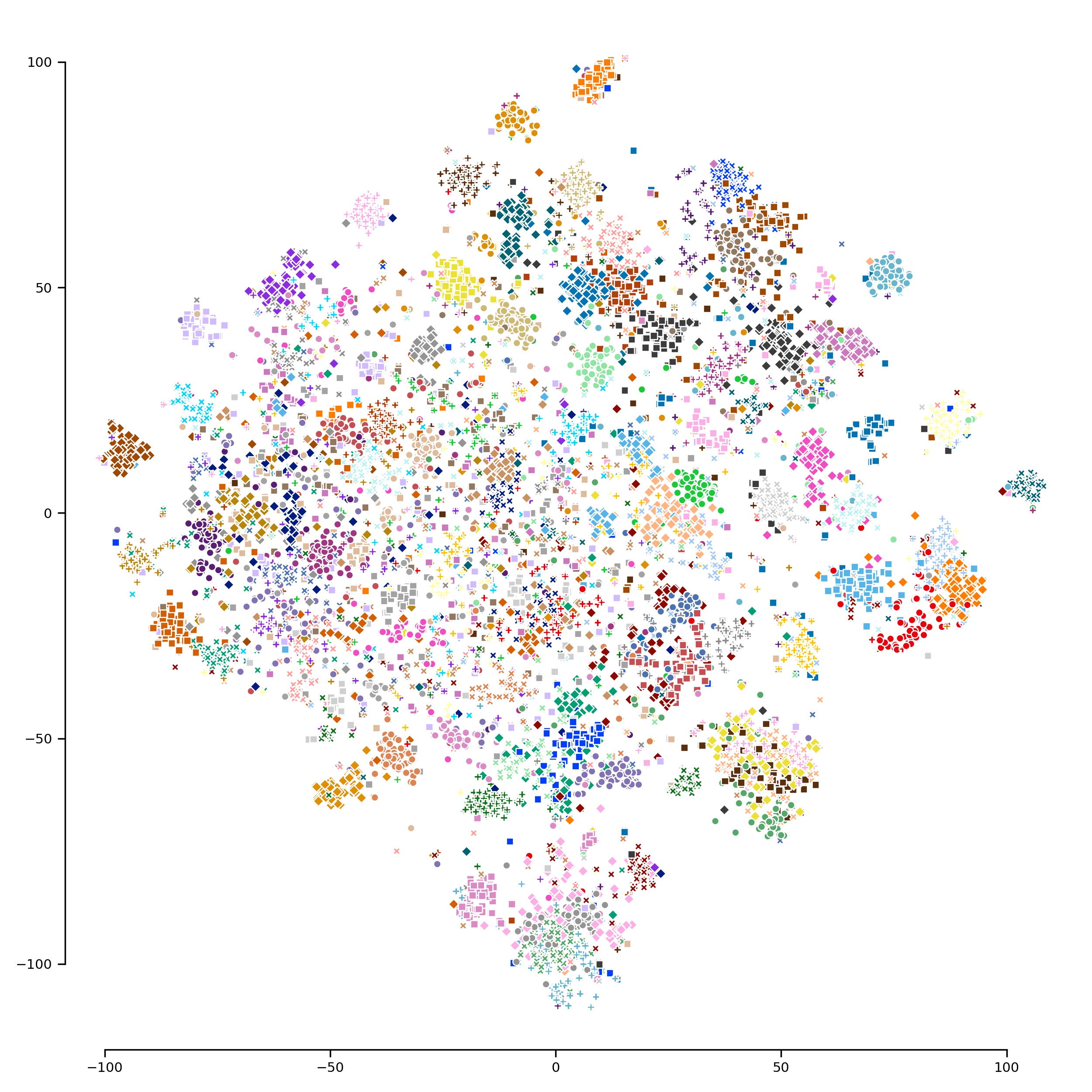
(a)

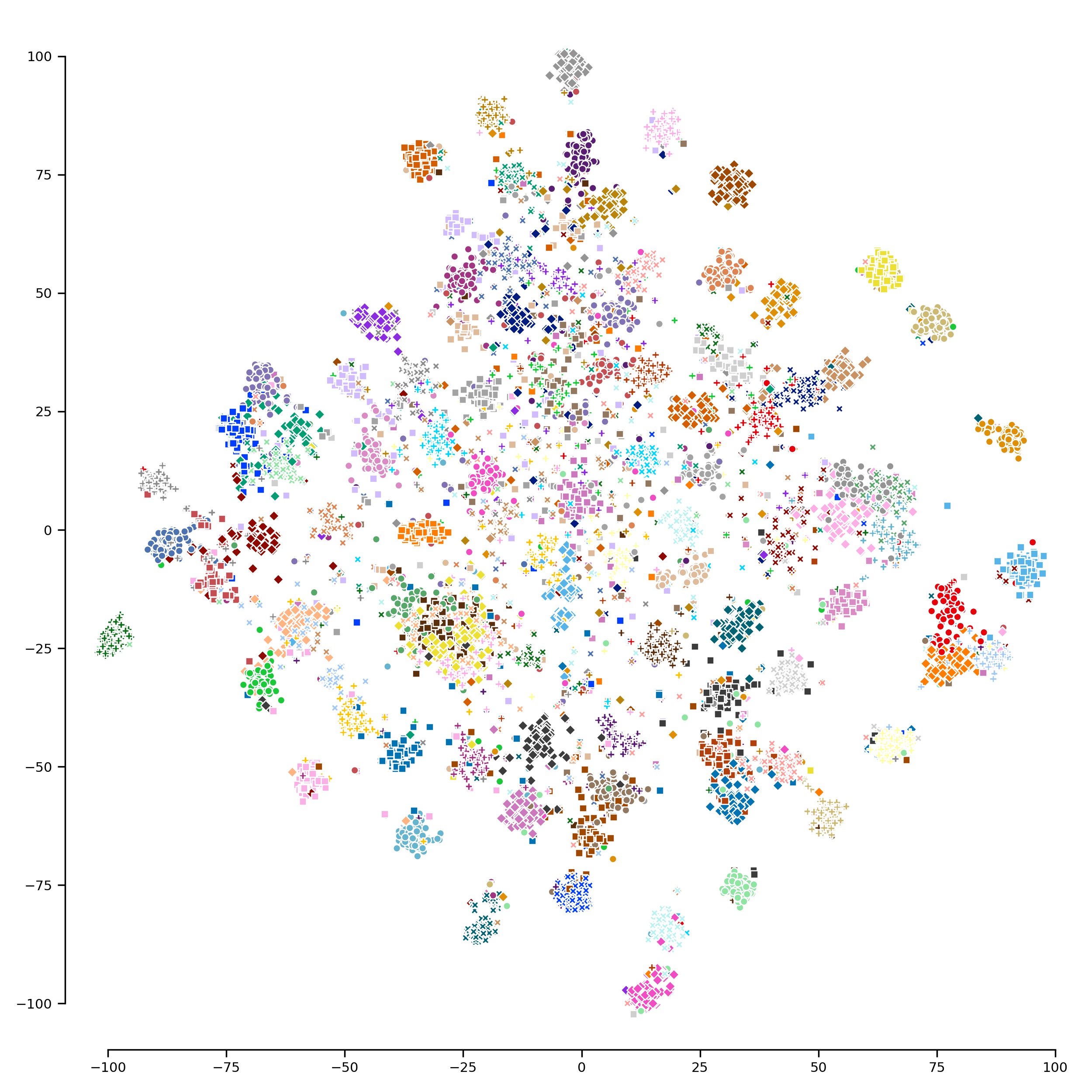
(b)

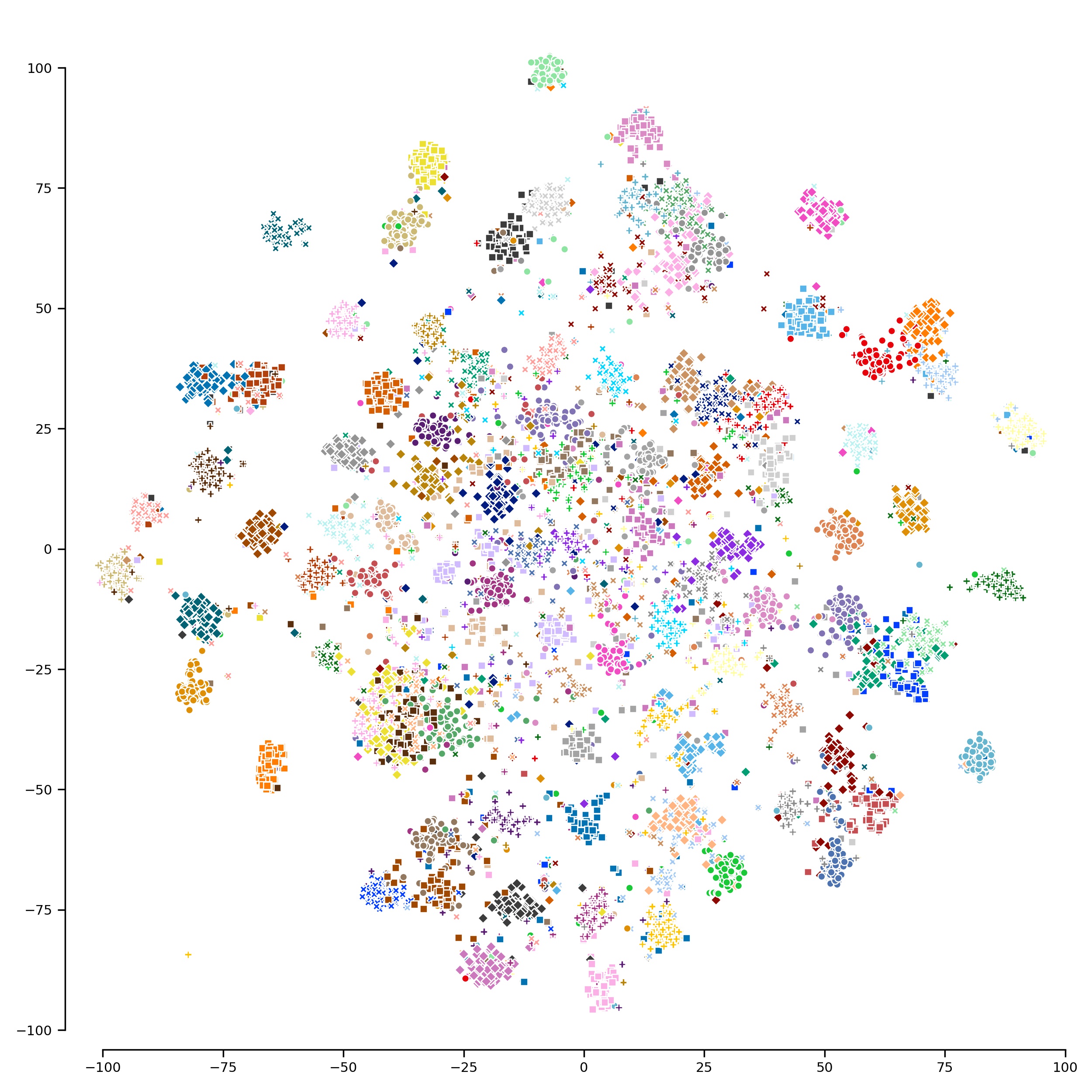
(c)

Figure 2: Qualitative comparison of embedding spaces. T-SNE plot of (a) supervised contrastive learning (SCL-in) and (b) RINCE-in (c) RINCE-out-in on Cifar-100. Best seen in color, on screen and zoomed in. Color and marker type combined indicate class. Labels omitted for clarity. Sup. Mat. contains a version of this plot with color indicating the superclass. RINCE learns a more structured embedding space than SCL, e.g. classes are linearly separable and can be modelled well by a Gaussian.

Out-of-distribution Detection.

To further investigate the structure of the learned representation of RINCE we evaluate on the task of out-of-distribution detection (OOD). As argued in (Winkens et al. 2020), models trained with cross-entropy only need to distinguish classes and can omit irrelevant features. Contrastive learning differs, by forcing the network to distinguish between each pair of samples, resulting in a more complete representation. Such a representation is beneficial for OOD detection (Hendrycks et al. 2019; Winkens et al. 2020). Therefore, OOD performance can be seen as evaluation of representation quality beyond standard metrics like accuracy and retrieval. RINCE incentivizes the network to learn an even richer representation. Besides that, OOD benefits from good trade-off between alignment and uniformity, which RINCE manages well (Fig. 9 in Sup. Mat.).

We follow common evaluation settings for OOD (Lee et al. 2018; Liang, Li, and Srikant 2018; Winkens et al. 2020). Here Cifar-100 is used as the inlier dataset $\mathcal{D}_{\text{in}}$, Cifar-10 and TinyImageNet as outlier dataset $\mathcal{D}_{\text{out}}$. Note that Cifar-100 and Cifar-10 have disjoint labels and images. For both protocols we only use the test or validation images. Our models are identical to those in the previous section. Inspired by (Winkens et al. 2020), we follow a simple approach, and fit class-conditional multivariate Gaussians to the embedding of the training set. We use the log-likelihood to define the OOD-score. As a result, the likelihood to identify OOD-samples is high, if each in-class follows roughly a Gaussian distribution in the embedding space, compare Fig. 2(a) and 2(c). For evaluation, we compute the area under the receiver operating characteristic curve (AUROC), details in Sup. Mat.

Results and a comparison to the most related previous work is shown in Tab. 2. Note that we aim here to compare the learned representation space via RINCE to its counterparts, i.e. cross-entropy and SCL, but show well known methods as reference. Most importantly, RINCE clearly outperforms cross-entropy, all SCL variants, contrastive OOD and our own baselines using the identical OOD approach. Only, two-heads outperforms all other methods in the near OOD setting with $\mathcal{D}_{\text{out}}$: Cifar10. However, performance on all other settings is low, showing weak generalization. This underlines our hypothesis, that training with RINCE yields a more structured and general representation space. Comparing to related works, RINCE not only outperforms Contrastive OOD (Winkens et al. 2020) using the same architecture, but even approaches the $4\times$ wider ResNet on Cifar10 as $\mathcal{D}_{\text{out}}$. ODIN (Liang, Li, and Srikant 2018) and Mahalanobis (Lee et al. 2018) require samples labelled as OOD to tune parameters of the OOD approach. Here we evaluate in the more realistic setting without labelled OOD samples. Despite using significantly less information, RINCE is compatible with them and even outperforms them for $\mathcal{D}_{\text{out}}$: Cifar10.

Method		AUROC
	Accuracy	$\mathcal{D}_{\text{out}}$:	$\mathcal{D}_{\text{out}}$:
		ImageNet-100†	AwA2
Cross-entropy s.a.	83.94	79.076 $\pm$ 1.477	79.04
SCL-out	84.18	79.779 $\pm$ 1.274	79.05
RINCE-out-in	84.90	80.473 $\pm$ 1.210	80.73

Table 3: ImageNet-100 classification accuracy and OOD detection for $\mathcal{D}_{\text{in}}$: ImageNet-100, and $\mathcal{D}_{\text{out}}$: ImageNet-100^† and AwA2 (Xian et al. 2018). ImageNet-100^† denotes three ImageNet-100 datasets with non-overlapping classes.

Large Scale Data and Noisy Similarities

Additionally, we perform the same evaluations on ImageNet-100, a 100-class subset of ImageNet, see Tab. 3. Here, we use ResNet-18. We obtain the second rank classes for a given class via similarities of the RoBERTa (Liu et al. 2019) class name embeddings. In contrast to the previous experiments, where ground truth hierarchies are known, these similarity scores are noisy and inaccurate – yet it still provides valuable information to the model. We evaluate our model via linear classification on ImageNet-100 and two OOD tasks: AwA2 (Xian et al. 2018) as $\mathcal{D}_{\text{out}}$ and ImageNet-100^†, where we use the remaining ImageNet classes to define three non-overlapping splits and report the average OOD.

Result are shown in Tab. 3. Again, RINCE significantly improves over SCL and cross-entropy in linear evaluation as well as on the OOD tasks. This demonstrates 1) that RINCE can handle noisy rankings and 2) that RINCE leads to improvements on large scale datasets. Next, we move to an even less controlled setting and define a ranking based on temporal ordering for unsupervised video representation learning.

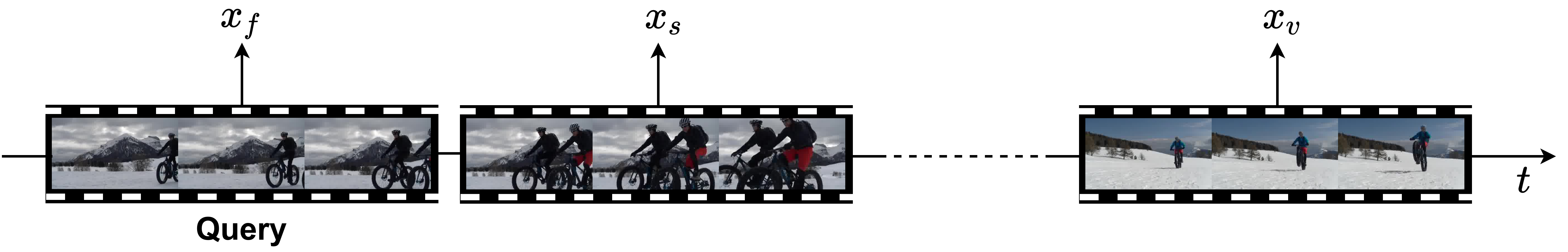
Figure 3: Positives in Videos. For a given query clip we use frame positives $x_{f}$, shot positives $x_{s}$ and video positives $x_{v}$.

Unsupervised RINCE

Method	Loss	Positives	Negatives	Top 1 Accuracy		Retrieval mAP
				HMDB	UCF	HMDB	UCF
VIE	-	-	-	$44.8$	$72.3$	-	-
LA-IDT	-	-	-	$44.0$	$72.8$	-	-
InfoNCE	$\mathcal{L}$	$\{x_{f}\}$	$\mathcal{N}$	$41.5$	$71.3$	$0.0500$	$0.0688$
hard positive	$\mathcal{L}^{\text{in}}$	$\{x_{f},x_{s},x_{v}\}$	$\mathcal{N}$	$42.6$	$74.3$	$0.0685$	$0.1119$
	$\mathcal{L}^{\text{out}}$	$\{x_{f},x_{s},x_{v}\}$	$\mathcal{N}$	$41.4$	$73.6$	$0.0666$	$0.1204$
easy positive	$\mathcal{L}^{\text{in}}$	$\{x_{f},x_{s}\}$	$\mathcal{N}$	$42.7$	$74.5$	$0.0581$	$0.1257$
	$\mathcal{L}^{\text{out}}$	$\{x_{f},x_{s}\}$	$\mathcal{N}$	$40.7$	$73.5$	$0.0593$	$0.1297$
hard negative	$\mathcal{L}^{\text{in}}$	$\{x_{f},x_{s}\}$	$\{x_{v}\}\cup\mathcal{N}$	$43.6$	$74.3$	$0.0678$	$0.1141$
	$\mathcal{L}^{\text{out}}$	$\{x_{f},x_{s}\}$	$\{x_{v}\}\cup\mathcal{N}$	$43.5$	$75.2$	$0.0675$	$0.1193$
RINCE	RINCE-uni	$x_{f}>x_{s}>x_{v}$	$\mathcal{N}$	$\mathbf{44.9}$	$\mathbf{75.4}$	$\mathbf{0.0719}$	$\mathbf{0.1395}$

Table 4: Finetuning on UCF and HMDB. $\mathcal{L}$, $\mathcal{L}^{\text{in}}$ and $\mathcal{L}^{\text{out}}$ correspond to Eq. (1), Eq. (3) and Eq. (2), respectively. Positives and Negatives indicates how $x_{f},x_{s},x_{v}$ were incorporated into contrastive learning, where $\mathcal{N}$ denotes the set of negative pairs from random clips. Since we consider only a single positive per rank we use the RINCE-uni loss variant for RINCE.

In this section we demonstrate that RINCE can be used in a fully unsupervised setting with noisy hierarchies by applying it to unsupervised video representation. Inspired by (Tschannen et al. 2020), we construct three ranks for a given query video, same frames, same shot and same video, see Fig. 3.

The first positive $x_{f}$ is obtained by augmenting the query frames. The second positive $x_{s}$ is a clip consecutive to the query frames, where small transformations of the objects, illumination changes, etc. occur. The third positive $x_{v}$ is sampled from a different time interval of the same video, which may show visually distinct but semantically related scenes. Naturally, $x_{f}$ shows the most similar content to the query frames, followed by $x_{s}$ and finally $x_{v}$. We compare temporal ranking with RINCE to different baselines.

Baselines.

We compare to the basic InfoNCE, where a single positive is generated via augmentations (Chen et al. 2020a; He et al. 2020), i.e. only frame positives $x_{f}$. When considering multiple clips from the same video such as $x_{s}$ and $x_{v}$, there are several possibilities: We can treat them all as positives (hard positive), we can use the distant $x_{v}$ as a hard negative or ignore it (easy positive). In both cases $\mathcal{L}^{\text{out}}$, Eq. (2), and $\mathcal{L}^{\text{in}}$, Eq. (3), are possible. Additionally, we compare to two recent methods trained in comparable settings, i.e. VIE (Zhuang et al. 2020), LA-IDT (Tokmakov, Hebert, and Schmid 2020).

Ranking Frame-, Shot- and Video-level Positives.

We sample short clips of a video, each consisting of $16$ frames. We augment each clip with a set of standard video augmentations. For more details we refer to the Sup. Mat. For the anchor clip $x$, we define positives as in Fig. 3: $p_{1}=x_{f}$ consists of the same frames as $x$, $p_{2}=x_{s}$ is a sequence of $16$ frames adjacent to $x$, and $p_{3}=x_{v}$ is sampled from a different time interval than $x_{f}$ and $x_{s}$. Negatives $x_{n}$ are sampled from different videos. Since each rank $i$ contains only a single positive $p_{i}$, Eq. (2) = Eq. (3), we call this variant RINCE-uni. By ranking the positives we ensure that the similarities satisfy $\text{sim}(x,x_{f})>\text{sim}(x,x_{s})>\text{sim}(x,x_{v})>\text{sim}(x,x_{n})$, adhering to the temporal structure in videos.

Datasets and Evaluation.

For self-supervised learning, we use Kinetics-400 (Kay et al. 2017) and discard the labels. Our version of the dataset consists of $234.584$ training videos. We evaluate the learned representation via finetuning on UCF (Soomro, Zamir, and Shah 2012) and HMDB (Kuehne et al. 2011) and report top 1 accuracy. In this evaluation, the pretrained weights are used to initialize a network and train it end-to-end using cross-entropy. Additionally, we evaluate the representation via nearest neighbor retrieval and report mAP. Precision-Recall curves can be found in the Sup. Mat.

Experimental Results.

For all experiments we use a 3D-ResNet-18 backbone. Training details can be found in the Sup. Mat. We report the results for RINCE as well as the baselines in Tab. 4. Adding shot- and video-level samples to InfoNCE improves the downstream accuracies. We observe that adding $x_{v}$ to the set of negatives to provide a hard negative rather than adding it to the set of positives leads to higher performance, suggesting that this should not be a true positive. This is further supported by the second and third row, where all three positives are treated as true positives. Here, $\mathcal{L}^{\text{out}}$, which forces all positives to be similar, leads to inferior performance compared to $\mathcal{L}^{\text{in}}$. $\mathcal{L}^{\text{in}}$ allows more noise in the set of positives by weak influence of false positives $x_{v}$. With RINCE we can impose the temporal ordering $x_{f}>x_{s}>x_{v}$ and treat $x_{v}$ properly, leading to the highest downstream performance. Improvements of RINCE over $\mathcal{L}^{\text{out}}$ is less pronounced on UCF. This is due to the strong static bias (Li, Li, and Vasconcelos 2018) of UCF and $\mathcal{L}^{\text{out}}$ encourages static features. Contrarily, improvements of RINCE over $\mathcal{L}^{\text{out}}$ on HMDB are substantial, due to the weaker bias towards static features. Last, we compare our method to two recent unsupervised video representation learning methods that use the same backbone network in Tab. 4. We outperform these methods on both datasets.

Conclusion

We introduced RINCE, a new member in the family of InfoNCE losses. We show that RINCE can exploit rankings to learn a more structured feature space with desired properties, lacking with standard InfoNCE. Furthermore, representations learned through RINCE can improve accuracy, retrieval and OOD. Most importantly, we show that RINCE works well with noisy similarities, is applicable to large scale datasets and to unsupervised training. We compare the different variants of RINCE. Here lies a limitation: Different variants are optimal for different tasks and must be chosen based on domain knowledge. Future work will explore further applications of obtaining similarity scores, e.g. based on distance in a pretrained embedding space, distance between cameras in a multi-view setting or distances between clusters.

Appendix A Appendix

RINCE Loss Analysis

In the following we will give a more theoretical analysis of RINCE, explain why it leads to ranking and justify our choice of setting $\tau_{i}<\tau_{i+1}$. First, we will study the relative penalty (Wang and Liu 2021) to identify which negatives contribute most to the individual RINCE terms, dependent on the choice of $\tau$ and elaborate how this results in ranking. Next, we will elaborate how the choice of $\tau_{i}<\tau_{i+1}$ guides the network towards a desired trade-off between the opposing terms in the RINCE loss.

Which loss term focuses on which negatives?

Following (Wang and Liu 2021), we investigate the impact of negatives in the loss relative to the impact of positives, which is referred to as relative penalty. The relative penalty $r_{n}^{p}$ is obtained by dividing the gradient magnitude with respect to the similarity of negative and query ($s_{q,n}=h(q,n)$) by the gradient magnitude with respect to the similarity of positive and query ($s_{q,p}=h(q,p)$):

$$r_{n}^{p}=\left|\frac{\partial\ell(q)}{\partial s_{q,n}}\right|/\left|\frac{\partial\ell(q)}{\partial s_{q,p}}\right|.$$ (6)

A large relative penalty for a given negative $n$ implies a large contribution of this negative in the InfoNCE loss. For simplicity, we consider only two ranks but extending the explanation to more ranks is trivial. Let $p_{1}\in\mathcal{P}_{1}$ denote a first rank positive, $p_{2}\in\mathcal{P}_{2}$ a second rank positive, $n\in\mathcal{N}$ a negative and capital letters denote the entire set. The relative penalty of a negative $n\in\mathcal{N}$ with respect to $p_{2}$ in $\ell_{2}$ is given by:

$$r_{n}^{p_{2}}=\frac{\exp(h(q,n)/\tau_{2})}{\sum\limits_{x\in\mathcal{N}\setminus\{n\}}\exp(h(q,x)/\tau_{2})}$$ (7)

Similarly, the relative penalty of $n$ with respect to $p_{1}$ in $\ell_{1}$ is:

$$r_{n}^{p_{1}}=\frac{\exp(h(q,n)/\tau_{1})}{\sum\limits_{x\in\mathcal{N}\setminus\{n\}}\exp(h(q,x)/\tau_{1})+\sum\limits_{p_{2}^{*}\in\mathcal{P}_{2}}\exp(h(q,p_{2}^{*})/\tau_{1})}\\$$ (8)

and for $p_{2}$ with respect to $p_{1}$ in $\ell_{1}$:

$$r_{p_{2}}^{p_{1}}=\frac{\exp(h(q,p_{2})/\tau_{1})}{\sum\limits_{x\in\mathcal{N}}\exp(h(q,x)/\tau_{1})+\sum\limits_{p_{2}^{*}\in\mathcal{P}_{2}\setminus\{p_{2}\}}\exp(h(q,p_{2}^{*})/\tau_{1})}.$$ (9)

Note that $p_{2}$ serves as a negative for $p_{1}$ in $\ell_{1}$ and a positive in $\ell_{2}$. With small $\tau_{1}$ Eq. (8) is larger for close samples of $n$ than with larger $\tau_{1}$. Therefore, small $\tau_{1}$ result in significantly larger relative penalties for $n$ close to $q$, in comparison to a larger $\tau_{1}$. Both also hold for Eq. (9) and $p_{2}$. Thus, increasing $\tau$ shifts the focus of the loss function from close negatives to a more uniform contribution of all negatives. With $\tau_{2}>\tau_{1}$, Eq. (7) is more uniform over different similarity scores than Eq. (8) and (9) (compare Fig. 3 in (Wang and Liu 2021)). Since $h(q,p_{2})>h(q,n)$ is enforced by the positive “pull force” in $\ell_{2}$, we have $r_{p_{2}}^{p_{1}}\gg r_{n}^{p_{1}}$. Therefore, higher emphasize is put on $h(q,p_{1})>h(q,p_{2})$ than on $h(q,p_{1})>h(q,n)$ in $\ell_{1}$ and, intuitively, $\ell_{2}$ emphasizes $h(q,p_{2})>h(q,n)$. Thus, $\ell_{1}$ ensures that $p_{1}$ and $p_{2}$ can be discriminated well and $\ell_{2}$ ensures discrimination between $p_{2}$ and $n$. In other words, with increasing rank, and thus increasing $\tau$, the focus of the loss gradually shifts from close negatives towards all negatives, effectively increasing with each rank the radius around $q$ at which significant relative penalty results from the negatives. This “pushing” force with gradual increasing radius from the respective negatives in combination with the pulling of the respective positives towards $q$ results in ranking.

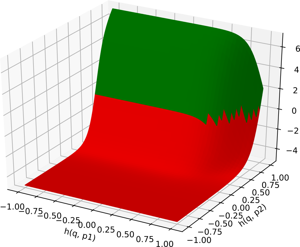
(a) $\tau_{1}=0.1,\tau_{2}=0.2$

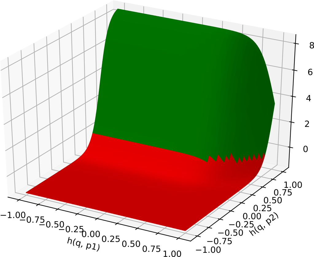
(b) $\tau_{1}=0.1,\tau_{2}=0.7$

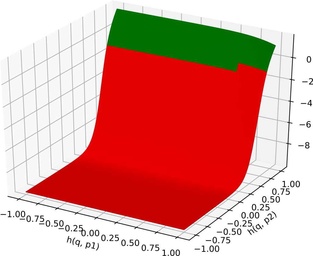
(c) $\tau_{1}=0.2,\tau_{2}=0.1$

Figure 4: Trade-off between opposing RINCE terms for varying $\tau_{1}$ and $\tau_{2}$. We visualize $\left|\frac{\partial\ell_{1}}{\partial p_{2}}\right|-\left|\frac{\partial\ell_{2}}{\partial p_{2}}\right|$ for different values of $h(q,p_{1})$ and $h(q,p_{2})$ ($h(q,n)$ is fixed). We show plots for different $\tau$ values. Red indicates negative values and green positive values. In the red region $h(q,p_{2})$ is maximized in the green region minimized. The equilibrium for a fixed $h(q,p_{1})$ lies on the boundary of red and green.

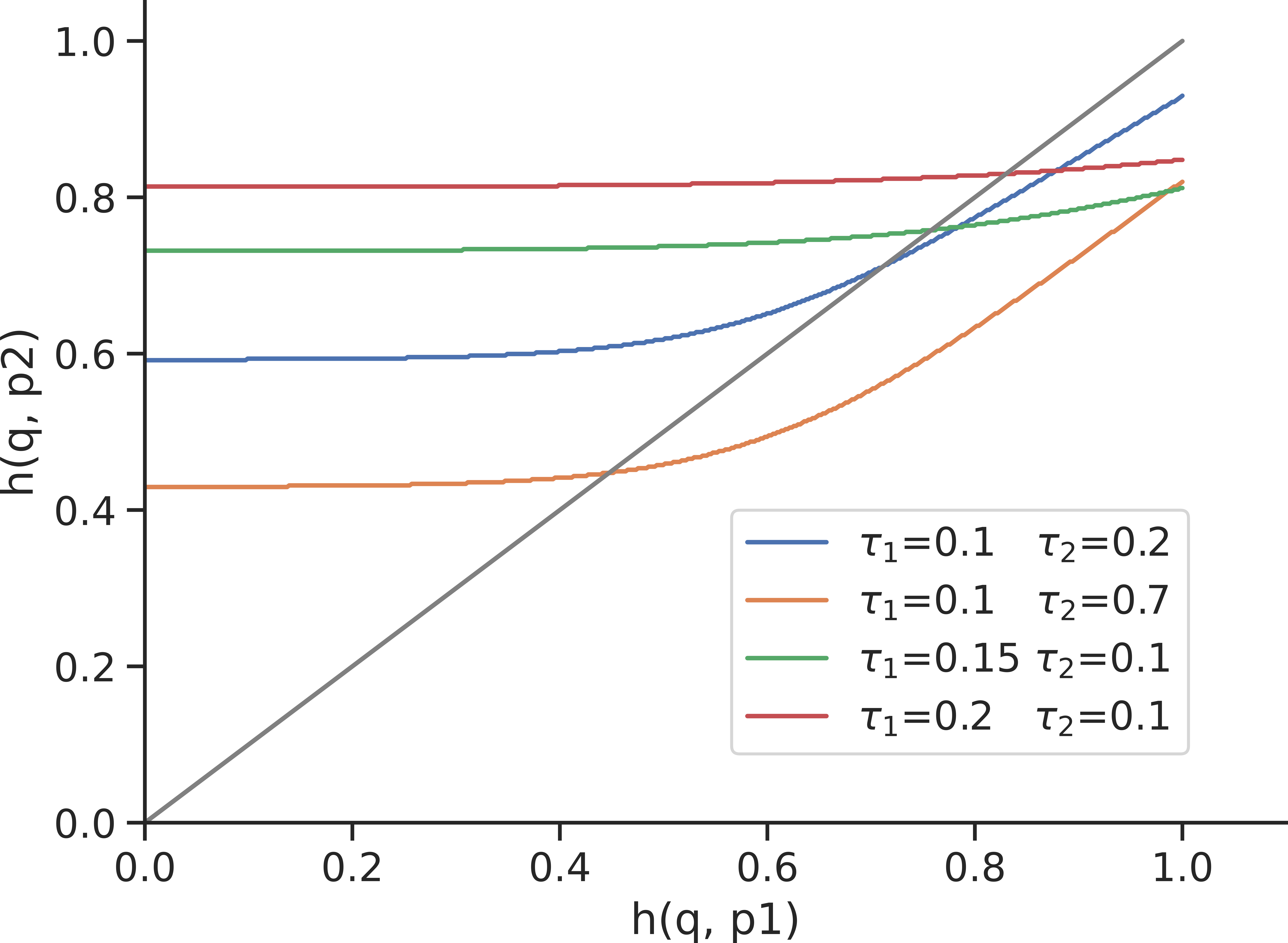
Figure 5: Equilibrium lines: Solutions for $K(h(q,p_{1}),h(q,p_{2}))=0$ for different values of $\tau_{1}$ and $\tau_{2}$. The lines show all combinations of $h(q,p_{1})$ and $h(q,p_{2})$ that are solutions of the opposing RINCE terms, i.e. the gradients are identical except for the sign. The grey line indicates $h(q,p_{1})=h(q,p_{2})$. For $\tau_{1}>\tau_{2}$ it can be seen that with increasing $\tau_{1}$, the curvature of the equilibrium line steadily decreases resulting in a almost constant value for $h(q,p_{2})$ for $\tau_{2}=0.2$.

RINCE-uni. In the RINCE-uni loss variant only a single positive is given for each rank, i.e. $\mathcal{P}_{i}=\{p_{i}\}$. In this case, we use Eq. (1) for the individual loss terms (Eq. (2) and Eq. (3) are the same for a single positive), and the loss reads:

$$\mathcal{L}_{\text{RINCE-uni}}=-\sum_{i=1}^{r}\log\frac{\exp(h(q,p_{i})/\tau_{i})}{\sum_{j=i}^{r}\exp(h(q,p_{j})/\tau_{i})+\sum_{n\in\mathcal{N}}\exp(h(q,n)/\tau_{i})}.$$ (10)

RINCE-out. For the RINCE-out loss variant we take the sum over positives outside of the $\log$ for each rank $i$:

$$\mathcal{L}_{\text{RINCE-out}}=-\sum_{i=1}^{r}\sum_{p\in\mathcal{P}_{i}}\log\frac{\exp(h(q,p)/\tau_{i})}{\sum_{p\in\{p_{i}\}\cup\left(\bigcup_{j>i}\mathcal{P}_{j}\right)}\exp(h(q,p)/\tau_{i})+\sum_{n\in\mathcal{N}}\exp(h(q,n)/\tau_{i})}.$$ (11)

RINCE-in. On the other hand, we take the sum over positives inside of the $\log$ for the RINCE-in loss variant:

$\displaystyle\mathcal{L}_{\text{RINCE-in}}=-\sum_{i=1}^{r}\log\frac{\sum_{p\in\mathcal{P}_{i}}\exp(h(q,p)/\tau_{i})}{\sum_{p\in\bigcup_{j\geq i}\mathcal{P}_{j}}\exp(h(q,p)/\tau_{i})+\sum_{n\in\mathcal{N}}\exp(h(q,n)/\tau_{i})}.$ (12)

Note that there is a subtle but noteworthy difference to the $\log$-in version of (Khosla et al. 2020), who compute the mean rather than the sum inside the $\log$. As they observe a significantly worse performance of their $\log$-in version, we decide to use the version proposed in (Miech et al. 2020; Han, Xie, and Zisserman 2020) for all our experiments, including the baseline SCL-in.

RINCE-out-in. Finally, we consider a combination of the two above: Whenever noise for first rank positives can be expected to be low, while it might be higher for higher rank positives we can use the out-option for the first rank and the in-option for the remaining ranks:

$\displaystyle\begin{split}\mathcal{L}_{\text{RINCE-out-in}}=-\sum_{p\in\mathcal{P}_{1}}\log\frac{\exp(h(q,p)/\tau_{1})}{\sum_{p\in\{p_{i}\}\cup\left(\bigcup_{j>1}\mathcal{P}_{j}\right)}\exp(h(q,p)/\tau_{1})+\sum_{n\in\mathcal{N}}\exp(h(q,n)/\tau_{1})}\\ -\sum_{i=2}^{r}\log\frac{\sum_{p\in\mathcal{P}_{i}}\exp(h(q,p)/\tau_{i})}{\sum_{p\in\bigcup_{j\geq i}\mathcal{P}_{j}}\exp(h(q,p)/\tau_{i})+\sum_{n\in\mathcal{N}}\exp(h(q,n)/\tau_{i})}.\qquad\quad\,\,\end{split}$ (13)

Table 5: Different RINCE loss variants. We assume that an ordered set of positives $\mathcal{P}_{1},\dots,\mathcal{P}_{r}$ is given, where $\mathcal{P}_{i}$ is the set of positives of rank $i$. We denote the set of negatives by $\mathcal{N}$.

How $\tau$ influences the optimal solution, controls the trade-off between opposing loss terms and why $\tau_{i}<\tau_{i+1}$ is a good choice for ranking.

To answer these question we study the trade-off mechanism between negatives in $\ell_{1}$ and the positives in $\ell_{2}$, i.e. the opposing terms in the RINCE loss that lead to the ranking. To investigate the trade-off, we compare the gradient with respect to the negatives $p_{2}$ in $\ell_{1}$ with the gradients with respect to the positives in $\ell_{2}$ (also $p_{2}$). We want to study which term dominates the entire gradient under which conditions. For this purpose we define

$$K(h(q,p_{1}),h(q,p_{2}))=\left|\frac{\partial\ell_{1}}{\partial p_{2}}\right|-\left|\frac{\partial\ell_{2}}{\partial p_{2}}\right|,$$ (14)

which is given by

$$\begin{split}&K(h(q,p_{1}),h(q,p_{2}))=\\ &\frac{1}{\tau_{1}}\frac{\exp(h(q,p_{2})/\tau_{1})}{\sum\limits_{n\in\mathcal{N}\cup\mathcal{P}_{2}}\exp(h(q,n)/\tau_{1})+\exp(h(q,p_{1})/\tau_{1})}\\ -&\frac{1}{\tau_{2}}\frac{\sum_{n\in\mathcal{N}}\exp(h(q,n)/\tau_{2})}{\sum\limits_{n\in\mathcal{N}}\exp(h(q,n)/\tau_{2})+\exp(h(q,p_{2})/\tau_{2})}\end{split}$$ (15)

Intuitively, the value of $K(h(q,p_{1}),h(q,p_{2}))$ in Eq. (14) shows which term dominates the gradient. In our case it even holds that $K(h(q,p_{1}),h(q,p_{2}))=\left|\frac{\partial\ell_{1}}{\partial p_{2}}\right|-\left|\frac{\partial\ell_{2}}{\partial p_{2}}\right|=\frac{\partial\ell_{1}}{\partial p_{2}}+\frac{\partial\ell_{2}}{\partial p_{2}}$, thus, $K(h(q,p_{1}),h(q,p_{2}))$ corresponds to the actual sum of the two gradients, meaning, that $K(h(q,p_{1}),h(q,p_{2}))=0$ means the gradients cancel each other out. There exist 3 different cases:

• $K>0$: $\left|\frac{\partial\ell_{1}}{\partial p_{2}}\right|>\left|\frac{\partial\ell_{2}}{\partial p_{2}}\right|$, i.e. $\frac{\partial\ell_{1}}{\partial p_{2}}$ dominates the gradient and effectively $\ell_{1}$ minimizes $h(q,p_{2})$.

• $K<0$: $\left|\frac{\partial\ell_{1}}{\partial p_{2}}\right|<\left|\frac{\partial\ell_{2}}{\partial p_{2}}\right|$, i.e. $\frac{\partial\ell_{2}}{\partial p_{2}}$ dominates the gradient and effectively $\ell_{2}$ maximizes $h(q,p_{2})$.

• $K=0$: An equilibrium between the opposing terms in $\ell_{1}$ and $\ell_{2}$ is found – neither $\frac{\partial\ell_{1}}{\partial p_{2}}$ nor $\frac{\partial\ell_{2}}{\partial p_{2}}$ dominates the gradient.

We visualize Eq. (14) in Fig. 4. To this end, we model $h(q,n)$ with a Gaussian with $\mu=0.1$ and $\sigma=0.1$ and show different combinations of $\tau$ values, namely $\tau_{1}=0.1,\tau_{2}=0.2$ in Fig. 4(a), $\tau_{1}=0.1,\tau_{2}=0.7$ in Fig. 4(b) and $\tau_{1}=0.2,\tau_{2}=0.1$ in Fig. 4(c). For convenience we color negative values in red and positive values in green. The equilibrium line separates red and green area. For easier comparison of the equilibrium lines, we visualize them in Fig. 5. It shows the value of $h(q,p_{2})$ that results in an equilibrium state as a function of $h(q,p_{1})$, i.e. it shows the projection of the equilibrium lines of Fig. 4 to the $h(q,p_{1}),h(q,p_{2})$ plane. We make the following observations:

1. For small values of $h(q,p_{1})$ the equilibrium line is close to constant – the optimization behavior of $h(q,p_{2})$ is not influenced by the values of $h(q,p_{1})$ – however, this only occurs very early in training, as $h(q,p_{1})$ is maximized without any opposing loss terms.

2. When $\tau_{1}<\tau_{2}$, the equilibrium line indicates that $h(q,p_{2})$ grows proportionately to $h(q,p_{1})$ (see Fig. 5 blue and orange).

3. When $\tau_{1}<\tau_{2}$, $h(q,p_{1})>h(q,p_{2})$ for the interesting regions (see  grey line in Fig. 5). $\tau_{2}$ can be used to control the minimal similarity of $h(q,p_{1})$ required for ranking to appear. Thus, higher ranks require larger $\tau_{2}$.

4. When increasing $\tau_{2}$ for a fixed $\tau_{1}$, the equilibrium line drops to smaller values overall – the trade-off is achieved with a smaller similarity of $h(q,p_{2})$ (compare Fig. 5). Again, this suits higher ranks better.

5. When $\tau_{1}>\tau_{2}$ the curvature of the equilibrium line decreases steadily. For example, with $\tau_{1}=0.2$ and $\tau_{2}=0.1$ it is almost constant. The optimization of $h(q,p_{2})$ is barely influenced by the values of $h(q,p_{1})$ (see green and red line in Fig. 5).

Aside from our theoretical justification, we empirically demonstrate that our loss preserves the desired ranking in the feature space, see Fig. 7.

RINCE Loss Variants

We discussed different RINCE loss variants in the main paper. Tab. 5 states the exact equations for the RINCE versions introduced in Tab. 1.

Computational Cost

RINCE only adds a small computational cost to the training pipeline, as only $r-1$ additional computations of the NCE loss function (Eq. (1)) are necessary. Note, that the dot products of $q$ and all $p\in P$ have to be computed only once and the respective results can be reused for each rank specific loss $\ell_{i}$ (Eq. (5)). In our experiments we did not observe a noticeable difference in overall training time between RINCE and SCL.

Hardware details

Experiments were performed on Nvidia GeForce 1080ti (12GB) and V100 GPUs (32GB), dependent on the respective memory requirements of the models. Contrastive learning for models in the supervised experiment section trained on Cifar-100 use a single V100 GPU, while evaluation, i.e. training a linear layer, retrieval and OOD experiments use the GeForce 1080ti GPUs. The experiments on ImageNet-100 were run on a V100 GPU. For models in the unsupervised experiments we use a single V100 GPU. The Bosch Group is carbon neutral. Administration, manufacturing and research activities do no longer leave a carbon footprint. This also includes GPU clusters on which the experiments have been performed.

Datasets

TinyImageNet (Le and Yang 2015) is a small version of ImageNet (Deng et al. 2009) comprising only 200 of the 1000 classes with each 500 samples at 64$\times$64 pixel resolution. ImageNet-100 (Tian, Krishnan, and Isola 2020) is a subset of ImageNet, consisting of 100 classes of ImageNet at full resolution. We use the RoBERTa (Liu et al. 2019) model to obtain semantic word embeddings for all class names in ImageNet-100. Second rank positives are based on the word embedding similarity and a predefined threshold.

Ranking for ImageNet-100.

To obtain ranking for ImageNet-100 we make use of recent progress in natural language processing. We use the RoBERTa (Liu et al. 2019) implementation provided by (Reimers and Gurevych 2019) trained for the semantic textual similarity benchmark (STSb) (Cer et al. 2017). We use this model to embed each class name into a $1024$ dimensional embedding space. Class similarities are computed for each pair using the cosine similarity. A small ablation of the robustness to the similarity score threshold is shown in Tab. 6. The accuracy is relatively robust on the choice of this threshold. We find $0.45$ to give the best results and use it for the experiments in the main paper.

Rank2 threshold	Accuracy	AUROC
$0.35$	$\mathbf{59.78}$	$60.92$
$0.40$	$59.40$	$61.80$
$0.45$	$59.44$	$\mathbf{62.92}$
$0.50$	$59.01$	$62.05$
$0.55$	$58.27$	$60.54$

Table 6: Ablation study on the RoBERTa word similarity threshold on TinyImageNet. We use different thresholds to define the rank 2 positives. We use RINCE-out-in for pretraining and report accuracy of linear evaluation and AUROC for OOD.

Supervised Contrastive Learning – Training Details

Our experiments are based on the Pytorch implementation of (Khosla et al. 2020). Common hyper-parameters are used, as given by (Khosla et al. 2020). We use ResNet-50 for all models trained on Cifar-100. For ImageNet-100 we use ResNet-18. During contrastive training we use a projection head with a single hidden layer with dimension of $2048$ and an output dimension of $128$.

Optimizer.

For both, SCL and RINCE we use stochastic gradient descent with a learning rate of $0.5$, batch size of $512$, momentum of $0.9$, weight decay of $1\mathrm{e}-4$ and a cosine learning rate scheduler. All models are trained for $1000$ epochs. $500$ epochs lead to slightly worse results and results do not change significantly when training for $2000$ instead of $1000$ epochs. Baselines using cross-entropy loss are trained only for $500$ epochs, as we observed that accuracy decreases after epoch $500$. For cross-entropy we use a learning rate of $0.8$, following (Khosla et al. 2020). In contrast to (Khosla et al. 2020) we use a batch size of $512$. We also tested the square root scaling rule for the learning rate, as proposed in (Krizhevsky 2014), but achieve lower accuracy. Our accuracy matches the one reported by (Khosla et al. 2020), despite the smaller batch size.

For ImageNet-100 we use a batch size of $768$ and find a learning rate of $0.3$ to give best results for RINCE and cross-entropy. For SCL we find $0.325$ to give best results. We train all models for $500$ epochs.

Data augmentation.

We use the same set of standard data augmentations as (Khosla et al. 2020) in their Pytorch implementation. We create a random crop of size between $20\%$ to $100\%$ of the initial image with random aspect ration between $3/4$ and $4/3$ of the initial aspect ratio. The resulting crop is scaled to $32\times 32$ pixels for Cifar-100 and $224\times 224$ for ImageNet-100. We flip images with a probability of $0.5$ and apply color jitter randomly selected from $[0.6,1.4]$ for brightness, contrast and saturation and apply jitter to the hue from $[-0.1,0.1]$ with a probability of $0.8$. Finally, we convert the image to grayscale with probability of $0.2$. Cross-entropy does not use color jitter and random grayscaling, but except from that uses the same augmentations. Cross-entropy strong augmentation (cross-entropy s.a.) uses the exact same augmentations as RINCE and SCL.

Memory bank and MoCo.

memorybank size	Accuracy
2048	77.03
4096	77.46
8092	77.25

Table 7: Ablation study on the size of the memorybank on Cifar-100. We use RINCE-out-in for pretraining and train a linear layer on top of the frozen network with cross-entropy.

To obtain a memory efficient solution, that can run on a single GPU we use a memory bank with the MoCo trick (He et al. 2020). Our search space for the memory bank size is inspired by the memory bank size used in an ablation study of (Khosla et al. 2020). Since we are training on Cifar-100 with only $100$ classes in comparison for $1000$ for ImageNet, we also try a smaller value. In initial experiments we compared three memory bank sizes: $2048$, $4096$ and $8192$, see Tab. 7. Differences were minor, but slightly better for $4096$. We use this value for all models trained on Cifar-100. For ImageNet-100 we use 8192, without further ablating it.

In MoCo training a second encoder network is used to get the representation for positives and negatives. The weights of this so-called key-encoder are a momentum-based moving average of the query encoder weights. We choose a value of $0.99$ as momentum, without further ablating it.

Temperature $\tau$.

Rank2 temperature	Accuracy
$\tau_{2}$=0.125	75.98
$\tau_{2}$=0.175	76.44
$\tau_{2}$=0.225	77.18
$\tau_{2}$=0.25	76.87

Table 8: Ablation study on $\tau_{2}$ on Cifar-100. We use RINCE-in for pretraining and train a linear layer on top of the frozen network with cross-entropy.

A critical parameter for the InfoNCE loss is the temperature $\tau$. RINCE requires determining a range of $\tau$ values. In practice, we found that starting with common values for $\tau_{1}$ and then linearly spacing $\tau_{i}$, $i>1$ works well. Effectively, this doubles the search effort. For SCL and RINCE we use the identical $\tau$ for rank 1. We tested $0.07$ and $0.1$ and found $0.1$ to work slightly better. For RINCE, a $\tau$ needs to be selected for each rank. For $\tau_{2}$ we searched for a good value over the range $[0.125,0.25]$ for RINCE-in, while keeping $\tau_{1}$ fixed to $0.1$. We found $\tau_{2}=0.225$ to work best. The corresponding ablation study on the sensitivity to the $\tau_{2}$ is shown in Tab. 8.

Randomness.

Whenever we provide mean and standard deviation we set the following random seeds: $123$, $546$ and $937$. We set them for Numpy and Pytorch individually.

	Classification Cifar-100			OOD
Smoothing factor	Accuracy	R@1 fine	R@1 superclass	$\mathcal{D}_{out}$: Cifar-10	$\mathcal{D}_{out}$: TinyImageNet
$\alpha=0.1$	75.66 $\pm$ 0.29	75.39 $\pm$ 0.33	85.42 $\pm$ 0.14	73.85 $\pm$ 0.19	80.04 $\pm$ 0.78
$\alpha=0.2$	75.66 $\pm$ 0.10	75.04 $\pm$ 0.06	85.38 $\pm$ 0.20	74.20 $\pm$ 0.23	79.84 $\pm$ 0.04
$\alpha=0.3$	75.66 $\pm$ 0.27	74.90 $\pm$ 0.06	85.59 $\pm$ 0.12	74.35 $\pm$ 0.65	80.10 $\pm$ 0.77

Table 9: Label Smoothing, effect of $\mathbf{\alpha}$. Hyper-parameter search for the smoothing factor $\alpha$, which determines how strongly the one-hot-vector is smoothed. We report the mean and standard deviation over three runs.

	Classification Cifar-100			OOD
loss weight	Accuracy	R@1 fine	R@1 superclass	$\mathcal{D}_{out}$: Cifar-10	$\mathcal{D}_{out}$: TinyImageNet
$\lambda=0.1$	73.85 $\pm$ 0.54	73.15 $\pm$ 0.80	81.37 $\pm$ 0.90	78.15 $\pm$ 0.49	77.91 $\pm$ 0.48
$\lambda=0.2$	74.08 $\pm$ 0.40	73.62 $\pm$ 0.31	81.92 $\pm$ 0.21	77.99 $\pm$ 0.07	78.35 $\pm$ 0.39
$\lambda=0.3$	74.05 $\pm$ 0.48	73.67 $\pm$ 0.29	82.39 $\pm$ 0.22	78.13 $\pm$ 0.11	78.97 $\pm$ 0.21

Table 10: Two heads: Effect of loss weight $\mathbf{\lambda}$. Hyper-parameter search for the loss weight $\lambda$, which controls how much the superclass classification contributes to the loss. We report the mean and standard deviation over 3 runs.

Training a linear layer.

After contrastive training we remove the MLP projection head and replace it with a single linear layer. We freeze the entire network, including the batch norm parameters and only train the weights of the linear layer with cross-entropy. For linear evaluation we use stochastic gradient descent with a learning rate of $5$ and a batch size of $512$ for Cifar-100 and for ImageNet-100. We decay the learning rate at epoch $60$, $75$ and $90$ with a decay rate of $0.2$.

Baselines – Supervised Contrastive Learning

Additionally to the SCL and cross entropy baselines, we provide 6 additional supervised baselines: label smoothing, two heads, SCL two heads, Triplet, Hierarchical triplet and Fast AP. The first two baselines are trained with cross-entropy. The hyper-parameters used are identical to those of the cross-entropy baseline. For SCL two heads we pick the same hyper-parameters as for SCL. Hyper-parameters that are new for the respective methods are determined with a parameter search. We always pick the model that results in highest accuracy after training a linear probe on top of the frozen features.

Label smoothing.

Label smoothing simply converts the one-hot-vectors used as target in the cross-entropy loss into a probability distribution over the target labels by assigning some of the probability to the other labels. In contrast to basic label smoothing and to use the same information as provided to RINCE, i.e. which classes belong to the same superclass, we do not distribute the probability mass to all classes, but only to those within the same superclass. Within the superclass we distribute the probability mass uniformly. A critical parameter is the smoothing factor $\alpha$, which denotes the fraction of the probability mass removed from the target class and distributed among the remaining classes. We tested three values and picked the one resulting in best accuracy on Cifar-100. All models are shown in Tab. 9.

Two heads.

The second simple baseline we compare to is referred to as two heads. To make use of the information provided by the superclasses we add a second classification head to the ResNet-50 backbone. While the first head is trained as before for fine label classification on Cifar-100, the second head is trained to predict the superclass labels. The loss is given by $\mathcal{L}=(1-\lambda)\mathcal{L}_{\text{fine}}+\lambda\mathcal{L}_{\text{superclass}}$. Critical is the weighting parameter $\lambda$. To find a good value we ran a small hyper-parameter search. The results are shown in Tab. 10. Again, we picked the model with highest classification accuracy on Cifar-100 fine labels for the main paper. Note, that $\lambda=0.1$ leads to best OOD scores on $\mathcal{D}_{out}$: Cifar-10, however, results on classification and retrieval are below vanilla cross-entropy (compare Tab. 2).

SCL two heads.

		Classification Cifar-100			OOD
	loss weight	Accuracy	R@1 fine	R@1 superclass	$\mathcal{D}_{out}$: Cifar-10	$\mathcal{D}_{out}$: TinyImageNet
SCL-in	$\lambda=0.1$	75.92	72.76	81.67	74.93	77.95
	$\lambda=0.2$	76.91	76.91	74,40	75.26	79.55
	$\lambda=0.3$	76.97	74.46	83,39	75.36	79.11
	$\lambda=0.4$	76.44	75.07	84.02	75.83	79.52
SCL-out	$\lambda=0.1$	75.94	72.76	81.67	74.93	77.95
	$\lambda=0.2$	75.82	73.68	82.25	75.26	79.74
	$\lambda=0.3$	76.47	74.36	83.27	74.52	79.00
	$\lambda=0.4$	76.89	74.37	83.60	74.98	79.33
	$\lambda=0.5$	76.32	75.09	84.02	75.76	79.86

Table 11: SCL two heads: Effect of loss weight $\mathbf{\lambda}$. Hyper-parameter search for the loss weight $\lambda$, which controls how much the superclass classification contributes to the loss.

Similarly, as for two heads, for SCL two heads we train simultaneously on fine and coarse labels. Instead of using cross-entropy we use the SCL loss. We follow the normla SCL setting with a projection head. In contrast to SCL we add a second projection head. The first head is trained like SCL on the fine labels, while the second is trained on the superclass labels. Similar to two heads, the loss is given by $\mathcal{L}=(1-\lambda)\mathcal{L}_{\text{fine}}+\lambda\mathcal{L}_{\text{superclass}}$. Ablation on hyper-parameter $\lambda$ can be found in Tab. 11.

Triplet Loss.

We use the triplet margin loss given by

$$\mathcal{L}_{\text{triplet}}=\text{max}\{d(q,p)-d(q,n)+m,0\},$$ (16)

where $d(\cdot,\cdot)$ is the euclidean distance and $m$ the margin. We adapt it to the ranking setting by choosing different margins based on the rank, We find $m_{1}=0.5$ and $m_{2}=1$ to work best in our setting. Further, we find a learning rate of $0.75$ to yield best results.

Hierarchical Triplet.

Hierarchical Triplet (Ge 2018) is a method for supervised learning. With the goal of hard example mining, the method learns a class hierarchy and draws samples from similar classes more frequently than dissimilar ones. Besides that, Hierarchical Triplet defines an adaptive violate margin, which depends on the class hierarchy. For a fair comparison to our setting, we do not learn the hierarchy. Instead, we use the ground truth hierarchy given by the Cifar-100 superclasses, similar as for RINCE. We use a batch size of $512$.

Hierarchical triplet performs hard example mining by sampling related classes with higher probability. Hard example mining is controlled with the following parameters: $l^{\prime}$ denotes the number of random classes per batch, $c$ denotes the number of samples drawn from the closest class for each sample and $t$ denotes the number of randomly drawn samples. Thus, $\text{batch\_size}=l^{\prime}+l^{\prime}c+t$. We find $l^{\prime}=30$, $c=10$ and $t=182$ to work well.

Fast AP.

Fast AP (Cakir et al. 2019) is a metric learning method tailored towards learning to rank. The loss directly optimizes Average Precision (AP) and is shown to result in high retrieval scores. The method uses differential histogram binning to efficiently approximate AP. Besides that, it introduces a special batch sampling strategy, which first samples categories (Cifar superclasses) and then for each category a number of samples (Cifar fine labels). We stick to the sampling strategy as proposed in the paper and sample per batch 2 categories. We ran a hyper-parameter search on the number of histogram bins and the learning rate. We found 5 histograms and a learning rate of 0.1 to work best in our setting. The remaining training details are identical to RINCE and the other baselines reported in this paper.

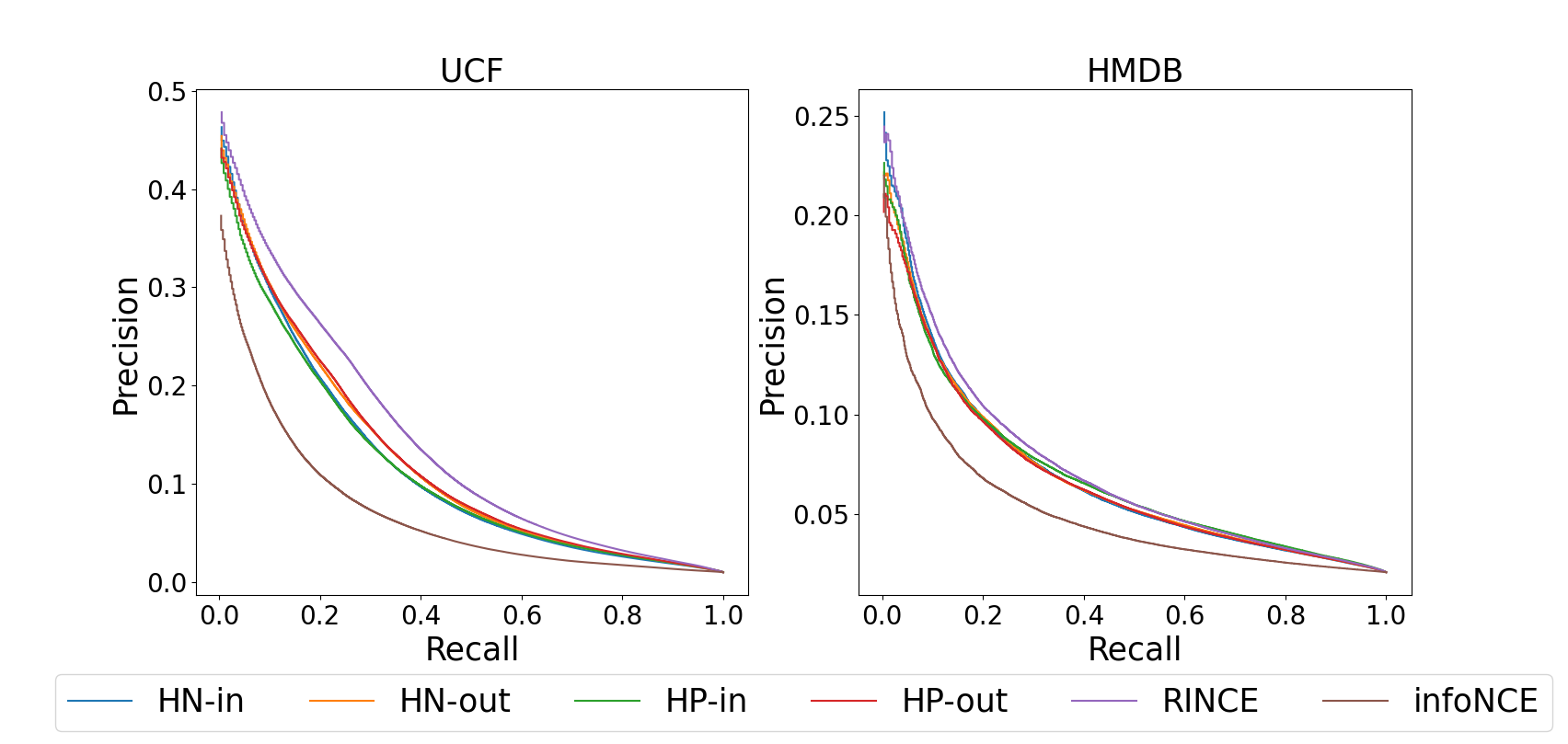
Figure 6: Precision-Recall Curves on UCF and HMDB. We show the precision-recall curves for the InfoNCE baseline, hard negatives (HN), hard positives (HP) and RINCE on the two action recognition datasets UCF and HMDB. We observe that both the in- and out-option of HN and HP improve over InfoNCE, while RINCE performs best.

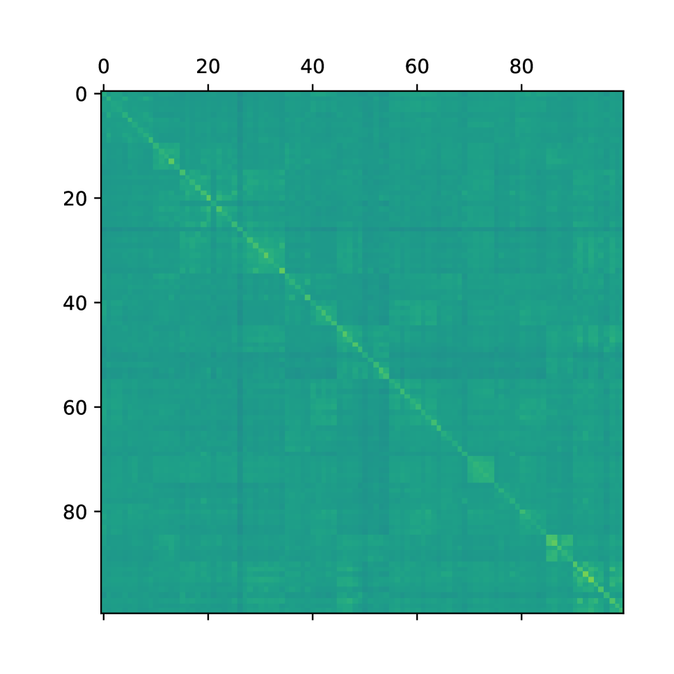
(a) SCL-in before MLP

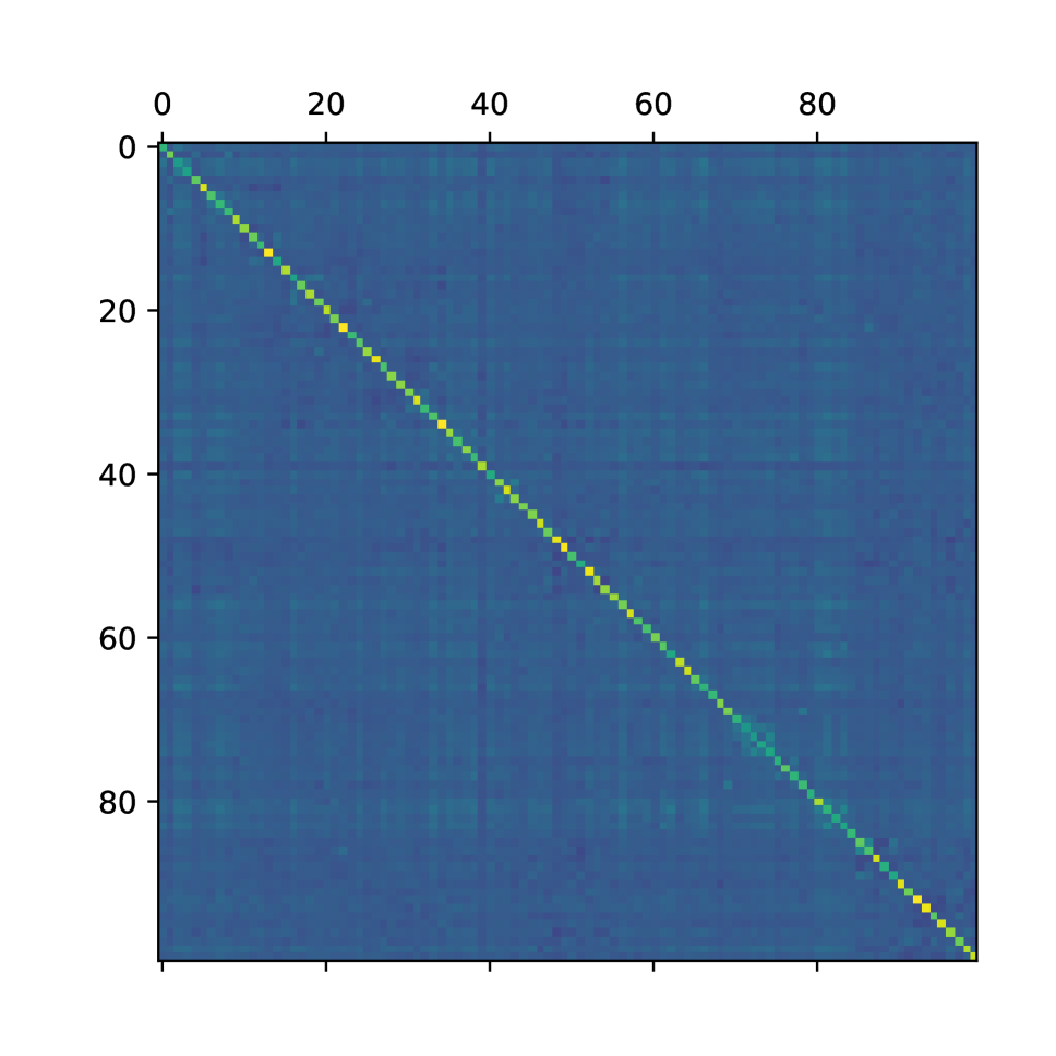
(b) SCL-in after MLP

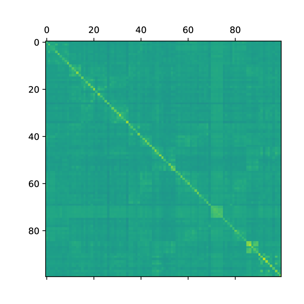
(c) RINCE-in before MLP

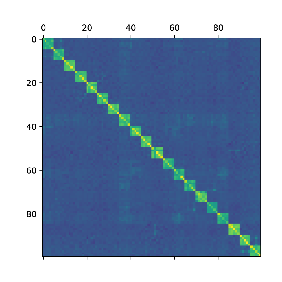
(d) RINCE-in after MLP

Figure 7: Similarity matrix on Cifar-100 classes before and after the MLP head. Classes are sorted, such that superclasses are grouped together. Similarity values are the average cosine similarity between classes. Similarity is larger for RINCE after the MLP, therefore ranking is learned by the MLP.

Out-of-Distribution Detection

After training we follow the setup of (Winkens et al. 2020) and fit $C$ $n$-dimensional class-conditional multivariate Gaussian to the embedded training samples with (Pedregosa et al. 2011), where $n$ is the dimension of the embedding space and $C$ denotes the number of classes in $\mathcal{D_{\text{in}}}$. The OOD score is defined as

$$s(x)=\max_{c}(\log(\textit{L}_{c}(x))),$$ (17)

where $\textit{L}_{c}$ denotes the likelihood function of the Gaussian for class $c$. Note, that this approach does not require any data labelled as OOD sample and can be applied out-of-the-box. We use this approach for all our baselines, i.e. cross-entropy, label smoothing, two-heads, SCL-in superclass, SCL-in and SCL-out.

For evaluation, we compute the area under the receiver operating characteristic curve (AUROC). Note that this metric is independent of any threshold and can be directly used on the OOD-scores. An intuitive interpretation of this metric is as the probability that a randomly picked in-distribution sample gets a higher in-distribution score than an OOD sample.

Unsupervised RINCE – Video Experiment

Implementation details.

We use a 3D-Resnet18 backbone (Hara, Kataoka, and Satoh 2018) in all experiments and pool the feature map into a single $512$-dimensional feature vector. The MLP head $g$ has $512$ hidden units with ReLu activation. Note that the MLP head is removed after self-supervised training and will not be transferred to downstream tasks. We use the Adam optimizer (Kingma and Ba 2015) with weight decay $1\mathrm{e}{-5}$, a batch size of $128$ and an initial learning rate of $1\mathrm{e}{-3}$, that is decreased by a factor of $10$ when the validation loss plateaus, and train for $200$ epochs. We use a memory bank size of $65.536$ (He et al. 2020) and do the momentum update with $m=0.99$. We use a temperature parameter $\tau=0.1$ for the baselines (InfoNCE, hard positives, hard negatives) and $\tau_{1}=0.1,\tau_{2}=0.15,\tau_{3}=0.2$ for RINCE.

Finetuning.

Downstream performances are reported on split 1 of UCF and HMDB. We use pretrained weights of the baselines and RINCE to initialize a 3D-Resnet18, add a randomly initialized linear layer and dropout with a dropout rate of $0.9$, and finetune everything end-to-end using cross entropy. We finetune the models for $500$ epochs using the Adam optimizer with weight decay $1\mathrm{e}{-5}$ and a learning rate of $1\mathrm{e}{-4}$ that is reduced by a factor of $10$ when the validation loss plateaus.

Frame-, Shot- and Video-level Positives.

We sample short clips each consisting of $16$ frames sampled with a temporal stride of $3$ for $x_{f}$, $x_{s}$ and $x_{v}$. We ensure a gap of at least $48$ frames between $x_{v}$ and the other two positives $x_{f}$ and $x_{s}$. We augment each clip with a set of standard video augmentations: random sized crop of size $128\times 128$, horizontal flip, color jittering and random color drop.

Precision-Recall Curves on UCF and HMDB.

We do the same retrieval evaluation as previously described for videos of UCF and HMDB and provide the resulting precision-recall curves in Fig. 6. We observe that the hard positive (HP) and hard negative (HN) baselines improve over InfoNCE, and RINCE outperforms all baselines. This is in line with our findings in Tab. 4.

Does RINCE rank samples?

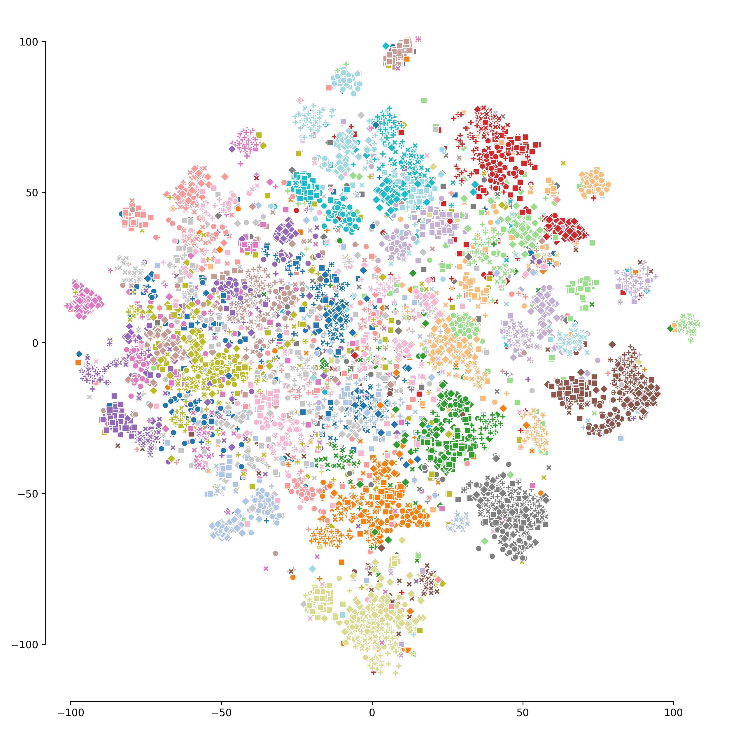
(a) SCL-in

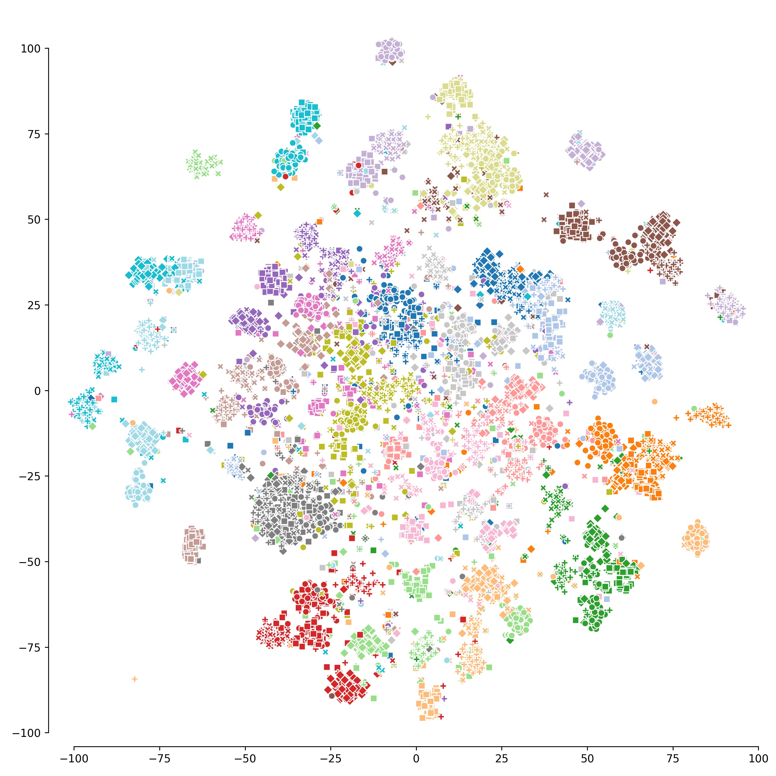
(b) RINCE-out-in

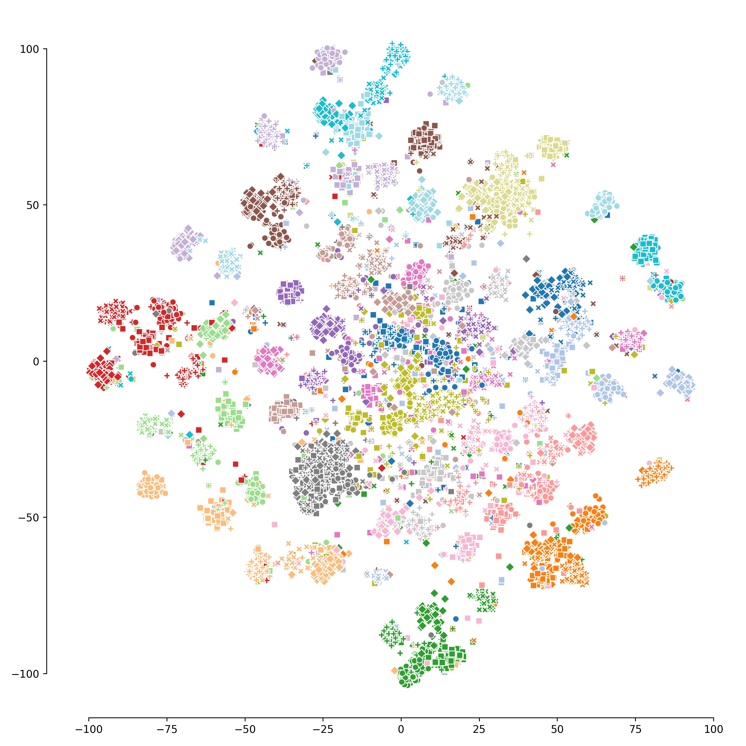
(c) RINCE-out

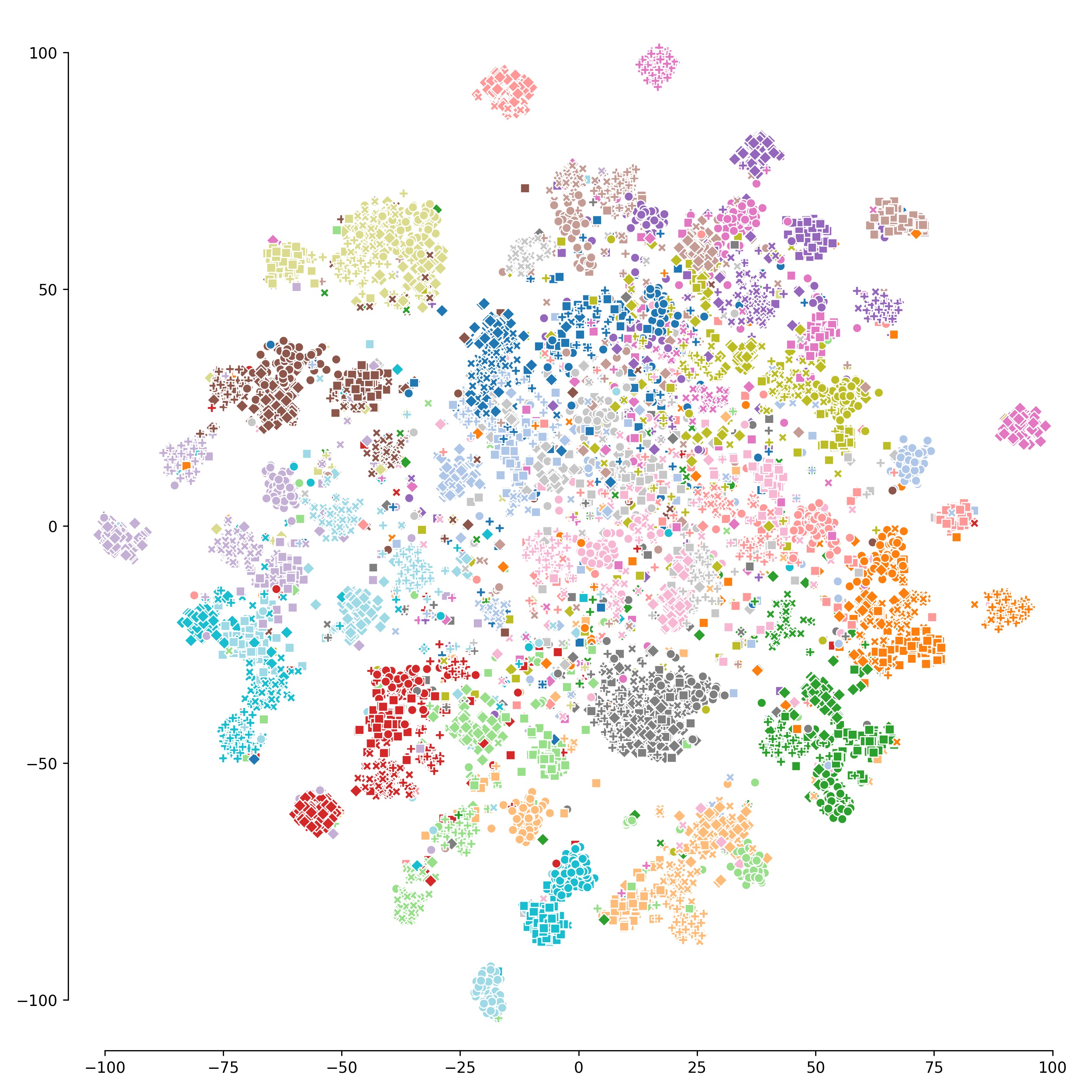
(d) Cross-entropy strong aug.

Figure 8: Alternative version of Fig. 2. Here superclasses have the same color and within a superclass the marker type denotes the class label (best viewed on screen and zoomed in). T-sne plot (Van der Maaten and Hinton 2008) of entire CIFAR-100 test set. For (a) supervised contrastive learning and (b) RINCE-out-in. (c) RINCE-out. (d) Cross-entropy strong aug.

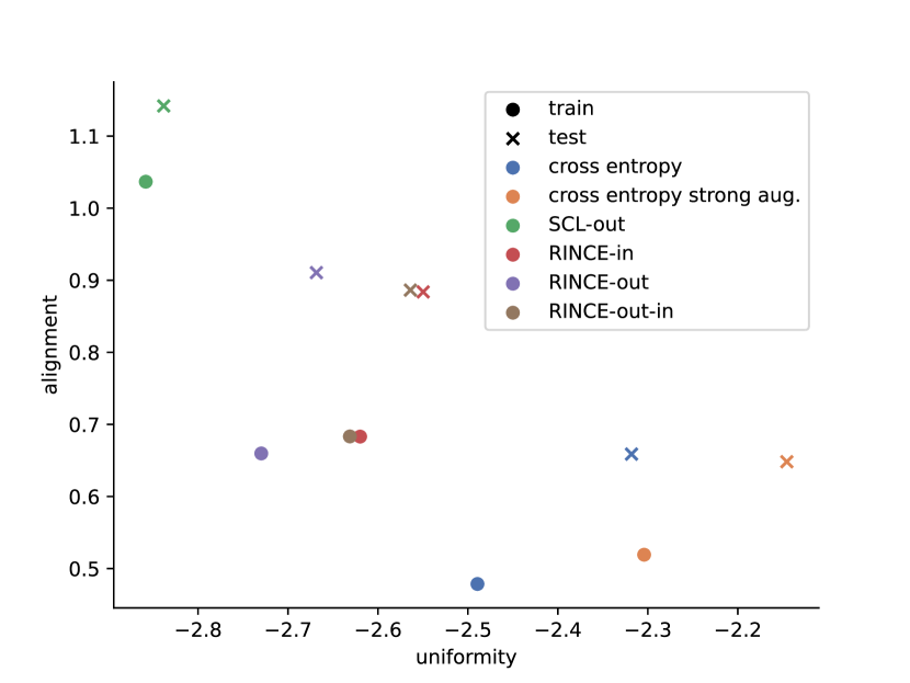
(a)

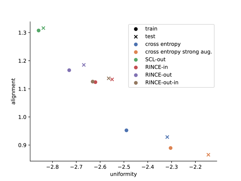
(b)

Figure 9: Alignment and uniformity for various models trained on Cifar-100. Methods with both, low alignment and low uniformity scores tend to generalize better to new downstream tasks (Wang and Isola 2020), thus best models are close to the bottom left. Alignment and uniformity computed on Cifar-100 train and test data for (a) fine labels and (b) for coarse labels. We compute alignment and uniformity before the MLP.

The experiments in the main paper show that RINCE leads to emergence of a well structured embedding space with useful properties, but whether RINCE learns to rank was evaluated only indirectly. To empirically validate that our method preserves the desired ranking we compute the average cosine distance between classes. If ranking is encoded in the embedding, highest similarity should be seen for same class, second highest for samples from the superclasses and low similarity for others. We visualize the results as similarity matrix in Fig. 7. It can be seen that RINCE-in does learn the ranking to some extent in the embedding space (Fig. 7(c)). Differences become more apparent after the MLP head. Here superclasses show high similarity, which however, does not approach the within-class-similarity (compare Fig. 7(c) and 7(d)). This shows that ranking is implemented to a large extent in the MLP. SCL-in also tends to have slightly higher similarity within superclasses (Fig.7(a)), but after the MLP mostly within-class-similarity is preserved (Fig.7(b)). This observation confirms that Eq. (12) mirrors the desired ranking in the latent space. Enforcing such a structure in the output space, results in a better representation in the intermediate layer, as the previous layer should explore the underlying structure of data more intensively to provide the last layers of low capacity with enough information for the ranking.

T-SNE.

Fig. 8, depicts t-SNE plots. Color of the points denotes the superclasses of Cifar-100. Similar to the findings discussed in the previous section, it can be seen that SCL (Fig. 2(a)) does a relatively bad job clustering the superclasses together, while RINCE and cross-entropy tend to group same superclasses together.

Alignment and Uniformity

Another way to study the representations learned with RINCE is by examining how it influences the common alignment and uniformity metrics (Wang and Isola 2020). As shown in (Wang and Isola 2020), low alignment scores in combination with low uniformity scores correlate with high downstream task performance. We find that training with RINCE results in a better trade-off between alignment and uniformity, compared to cross-entropy and SCL (see Fig. 9(a)).

Training with RINCE extends the alignment property across multiple samples. Therefore, positives are close to other rank 1 positives (standard alignment) but positives are also relatively close to rank 2 positives without sacrificing too much uniformity (compare Fig. 9(b)). For normal InfoNCE the rank 2 positives can be very far, as can be seen by poor alignment for SCL in Fig. 9(b).

Connection to OOD.

Intuitively, very low uniformity (close to uniform distribution) will result in very low OOD detection. Too high alignment, on the other hand can only be achieved, by ignoring many features. These features might be important to either spot OOD samples or generalize to similar, unseen samples. As a result, to achieve high OOD accuracy with a density estimation based approach a good trade-off between alignment and uniformity must be found.

References

- Behrmann, Gall, and Noroozi (2021) Behrmann, N.; Gall, J.; and Noroozi, M. 2021. Unsupervised Video Representation Learning by Bidirectional Feature Prediction. In WACV.
- Burges et al. (2005) Burges, C.; Shaked, T.; Renshaw, E.; Lazier, A.; Deeds, M.; Hamilton, N.; and Hullender, G. 2005. Learning to Rank Using Gradient Descent. In ICML.
- Cakir et al. (2019) Cakir, F.; He, K.; Xia, X.; Kulis, B.; and Sclaroff, S. 2019. Deep metric learning to rank. In CVPR.
- Cao et al. (2007) Cao, Z.; Qin, T.; Liu, T.-Y.; Tsai, M.-F.; and Li, H. 2007. Learning to rank: from pairwise approach to listwise approach. In ICML.
- Caron et al. (2020) Caron, M.; Misra, I.; Mairal, J.; Goyal, P.; Bojanowski, P.; and Joulin, A. 2020. Unsupervised Learning of Visual Features by Contrasting Cluster Assignments. In NeurIPS.
- Cer et al. (2017) Cer, D.; Diab, M.; Agirre, E.; Lopez-Gazpio, I.; and Specia, L. 2017. Semeval-2017 task 1: Semantic textual similarity-multilingual and cross-lingual focused evaluation. arXiv preprint arXiv:1708.00055.
- Chen et al. (2020a) Chen, T.; Kornblith, S.; Norouzi, M.; and Hinton, G. 2020a. A Simple Framework for Contrastive Learning of Visual Representations. In ICML.
- Chen et al. (2020b) Chen, X.; Fan, H.; Girshick, R.; and He, K. 2020b. Improved baselines with momentum contrastive learning. arXiv:2003.04297.
- Chen and He (2021) Chen, X.; and He, K. 2021. Exploring simple siamese representation learning. In CVPR.
- Dave et al. (2021) Dave, I.; Gupta, R.; Rizve, M. N.; and Shah, M. 2021. TCLR: Temporal Contrastive Learning for Video Representation. arXiv preprint arXiv:2101.07974.
- Deng et al. (2009) Deng, J.; Dong, W.; Socher, R.; Li, L.-J.; Li, K.; and Fei-Fei, L. 2009. Imagenet: A large-scale hierarchical image database. In CVPR.
- Deselaers and Ferrari (2011) Deselaers, T.; and Ferrari, V. 2011. Visual and semantic similarity in imagenet. In CVPR.
- Dosovitskiy et al. (2016) Dosovitskiy, A.; Fischer, P.; Springenberg, J. T.; Riedmiller, M.; and Brox, T. 2016. Discriminative Unsupervised Feature Learning with Exemplar Convolutional Neural Networks. In TPAMI.
- Feichtenhofer et al. (2021) Feichtenhofer, C.; Fan, H.; Xiong, B.; Girshick, R.; and He, K. 2021. A Large-Scale Study on Unsupervised Spatiotemporal Representation Learning. In CVPR.
- Ge (2018) Ge, W. 2018. Deep metric learning with hierarchical triplet loss. In ECCV.
- Grill et al. (2020) Grill, J.-B.; Strub, F.; Altché, F.; Tallec, C.; Richemond, P.; Buchatskaya, E.; Doersch, C.; Avila Pires, B.; Guo, Z.; Gheshlaghi Azar, M.; Piot, B.; Kavukcuoglu, K.; Munos, R.; and Valko, M. 2020. Bootstrap Your Own Latent - A New Approach to Self-Supervised Learning. In NeurIPS.
- Han, Xie, and Zisserman (2020) Han, T.; Xie, W.; and Zisserman, A. 2020. Self-supervised Co-training for Video Representation Learning. In NeurIPS.
- Hara, Kataoka, and Satoh (2018) Hara, K.; Kataoka, H.; and Satoh, Y. 2018. Can Spatiotemporal 3D CNNs Retrace the History of 2D CNNs and ImageNet? In CVPR.
- He et al. (2020) He, K.; Fan, H.; Wu, Y.; Xie, S.; and Girshick, R. 2020. Momentum Contrast for Unsupervised Visual Representation Learning. In CVPR.
- Hendrycks et al. (2019) Hendrycks, D.; Mazeika, M.; Kadavath, S.; and Song, D. 2019. Using Self-Supervised Learning Can Improve Model Robustness and Uncertainty. NeurIPS.
- Huynh et al. (2020) Huynh, T.; Kornblith, S.; Walter, M. R.; Maire, M.; and Khademi, M. 2020. Boosting Contrastive Self-Supervised Learning with False Negative Cancellation. arXiv preprint arXiv:2011.11765.
- Kay et al. (2017) Kay, W.; Carreira, J.; Simonyan, K.; Zhang, B.; Hillier, C.; Vijayanarasimhan, S.; Viola, F.; Green, T.; Back, T.; Natsev, P.; Suleyman, M.; and Zisserman, A. 2017. The Kinetics Human Action Video Dataset. arXiv, abs/1705.06950.
- Khosla et al. (2020) Khosla, P.; Teterwak, P.; Wang, C.; Sarna, A.; Tian, Y.; Isola, P.; Maschinot, A.; Liu, C.; and Krishnan, D. 2020. Supervised Contrastive Learning. NeurIPS.
- Kingma and Ba (2015) Kingma, D.; and Ba, J. 2015. Adam: A method for stochastic optimization. In ICLR.
- Krizhevsky (2014) Krizhevsky, A. 2014. One weird trick for parallelizing convolutional neural networks. arXiv preprint arXiv:1404.5997.
- Krizhevsky, Hinton et al. (2009) Krizhevsky, A.; Hinton, G.; et al. 2009. Learning multiple layers of features from tiny images. Tech Report.
- Kuehne et al. (2011) Kuehne, H.; Jhuang, H.; Garrote, E.; Poggio, T.; and Serre, T. 2011. HMDB: A large video database for human motion recognition. In ICCV.
- Le and Yang (2015) Le, Y.; and Yang, X. 2015. Tiny imagenet visual recognition challenge.
- Lee and Cheon (2020) Lee, D.; and Cheon, Y. 2020. Soft Labeling Affects Out-of-Distribution Detection of Deep Neural Networks. arXiv preprint arXiv:2007.03212.
- Lee et al. (2018) Lee, K.; Lee, K.; Lee, H.; and Shin, J. 2018. A simple unified framework for detecting out-of-distribution samples and adversarial attacks. NeurIPS.
- Li, Li, and Vasconcelos (2018) Li, Y.; Li, Y.; and Vasconcelos, N. 2018. RESOUND: Towards Action Recognition without Representation Bias. In ECCV.
- Liang, Li, and Srikant (2018) Liang, S.; Li, Y.; and Srikant, R. 2018. Enhancing the reliability of out-of-distribution image detection in neural networks. In ICLR.
- Liu (2009) Liu, T.-Y. 2009. Learning to Rank for Information Retrieval. Foundations and Trends® in Information Retrieval.
- Liu et al. (2019) Liu, Y.; Ott, M.; Goyal, N.; Du, J.; Joshi, M.; Chen, D.; Levy, O.; Lewis, M.; Zettlemoyer, L.; and Stoyanov, V. 2019. Roberta: A robustly optimized bert pretraining approach. arXiv preprint arXiv:1907.11692.
- Miech et al. (2020) Miech, A.; Alayrac, J.-B.; Smaira, L.; Laptev, I.; Sivic, J.; and Zisserman, A. 2020. End-to-End Learning of Visual Representations from Uncurated Instructional Videos. In CVPR.
- Misra and van der Maaten (2020) Misra, I.; and van der Maaten, L. 2020. Self-Supervised Learning of Pretext-Invariant Representations. In CVPR.
- Neill and Bollegala (2021) Neill, J. O.; and Bollegala, D. 2021. Semantically-Conditioned Negative Samples for Efficient Contrastive Learning. arXiv preprint arXiv:2102.06603.
- Pedregosa et al. (2011) Pedregosa, F.; Varoquaux, G.; Gramfort, A.; Michel, V.; Thirion, B.; Grisel, O.; Blondel, M.; Prettenhofer, P.; Weiss, R.; Dubourg, V.; Vanderplas, J.; Passos, A.; Cournapeau, D.; Brucher, M.; Perrot, M.; and Duchesnay, E. 2011. Scikit-learn: Machine Learning in Python. JMLR.
- Reimers and Gurevych (2019) Reimers, N.; and Gurevych, I. 2019. Sentence-BERT: Sentence Embeddings using Siamese BERT-Networks. In EMNLP.
- Romijnders et al. (2021) Romijnders, R.; Mahendran, A.; Tschannen, M.; Djolonga, J.; Ritter, M.; Houlsby, N.; and Lucic, M. 2021. Representation Learning From Videos In-the-Wild: An Object-Centric Approach. In WACV.
- Sastry and Oore (2020) Sastry, C. S.; and Oore, S. 2020. Detecting out-of-distribution examples with gram matrices. In ICML.
- Sohn (2016) Sohn, K. 2016. Improved Deep Metric Learning with Multi-class N-pair Loss Objective. In NIPS.
- Soomro, Zamir, and Shah (2012) Soomro, K.; Zamir, A. R.; and Shah, M. 2012. UCF101: A dataset of 101 human actions classes from videos in the wild. arXiv, abs/1212.0402.
- Szegedy et al. (2016) Szegedy, C.; Vanhoucke, V.; Ioffe, S.; Shlens, J.; and Wojna, Z. 2016. Rethinking the inception architecture for computer vision. In CVPR.
- Tian, Krishnan, and Isola (2020) Tian, Y.; Krishnan, D.; and Isola, P. 2020. Contrastive Multiview Coding. In ECCV.
- Tian et al. (2020) Tian, Y.; Sun, C.; Poole, B.; Krishnan, D.; Schmid, C.; and Isola, P. 2020. What makes for good views for contrastive learning. arXiv preprint arXiv:2005.10243.
- Tokmakov, Hebert, and Schmid (2020) Tokmakov, P.; Hebert, M.; and Schmid, C. 2020. Unsupervised Learning of Video Representations via Dense Trajectory Clustering. In ECCV Workshops.
- Tschannen et al. (2020) Tschannen, M.; Djolonga, J.; Ritter, M.; Mahendran, A.; Houlsby, N.; Gelly, S.; and Lucic, M. 2020. Self-Supervised Learning of Video-Induced Visual Invariances. In CVPR.
- van den Oord, Li, and Vinyals (2018) van den Oord, A.; Li, Y.; and Vinyals, O. 2018. Representation Learning with Contrastive Predictive Coding. arXiv, abs/1807.03748.
- Van der Maaten and Hinton (2008) Van der Maaten, L.; and Hinton, G. 2008. Visualizing data using t-SNE. JMLR.
- Wang and Liu (2021) Wang, F.; and Liu, H. 2021. Understanding the Behaviour of Contrastive Loss. In CVPR.
- Wang and Isola (2020) Wang, T.; and Isola, P. 2020. Understanding contrastive representation learning through alignment and uniformity on the hypersphere. In ICML.
- Weinberger, Blitzer, and Saul (2006) Weinberger, K. Q.; Blitzer, J.; and Saul, L. 2006. Distance Metric Learning for Large Margin Nearest Neighbor Classification. In NIPS.
- Winkens et al. (2020) Winkens, J.; Bunel, R.; Roy, A. G.; Stanforth, R.; Natarajan, V.; Ledsam, J. R.; MacWilliams, P.; Kohli, P.; Karthikesalingam, A.; Kohl, S.; et al. 2020. Contrastive training for improved out-of-distribution detection. arXiv preprint arXiv:2007.05566.
- Xian et al. (2018) Xian, Y.; Lampert, C. H.; Schiele, B.; and Akata, Z. 2018. Zero-Shot Learning - A Comprehensive Evaluation of the Good, the Bad and the Ugly. In TPAMI.
- Zhao et al. (2021) Zhao, N.; Wu, Z.; Lau, R. W. H.; and Lin, S. 2021. What Makes Instance Discrimination Good for Transfer Learning? In ICLR.
- Zhuang et al. (2020) Zhuang, C.; She, T.; Andonian, A.; Mark, M. S.; and Yamins, D. 2020. Unsupervised Learning From Video With Deep Neural Embeddings. In CVPR.