Strong dispersion property for the quantum walk on the hypercube

Abstract

We show that the discrete time quantum walk on the Boolean hypercube of dimension $n$ has a strong dispersion property: if the walk is started in one vertex, then the probability of the walker being at any particular vertex after $O(n)$ steps is of an order $O(1.4818^{-n})$. This improves over the known mixing results for this quantum walk which show that the probability distribution after $O(n)$ steps is close to uniform but do not show that the probability is small for every vertex. Our result shows that quantum walk on hypercube is interesting for algorithmic applications which require fast dispersion over the state space.

Keywords: quantum walk, Boolean hypercube, dispersiveness

I Introduction

Quantum walks are the quantum counterpart of random walks. They have been very useful for designing quantum algorithms, from the exponential speedup for the “glued trees” problem by Childs et al. Childs et al. (2003) and the element distinctness algorithm of Ambainis (2007) to general results about speeding up classes of Markov chains Szegedy (2004); Apers and Sarlette (2019); Ambainis et al. (2020); Apers et al. (2021). Quantum walks also have applications to other areas (e.g. quantum state transfer Mohseni et al. (2008) or Hamiltonian complexity Nagaj et al. (2009)) and are interesting objects of study on their own.

One of most important properties of both classical random walks and quantum walks is rapid mixing Levin and Peres (2017); Randall (2006): if the walk is started in one vertex, after a certain number of steps the probability distribution of the walker is almost uniformly distributed over all vertices. Rapid mixing takes place for many graphs, the key condition for it is that the graph on which the walker is walking has no bottlenecks that may slow it down. Classically, rapid mixing is useful for a variety of algorithms that perform sampling, counting or integration (for example, algorithms for estimating volumes of convex bodies Dyer et al. (1991); Lovász and Vempala (2006)). Quantum walks also mix rapidly in many cases (e.g. Moore and Russell (2002)), for an appropriate definition of mixing and their mixing times can be related to the same combinatorial quantities of the underlying graph as classically Aharonov et al. (2001).

In this paper, we show that a popular quantum walk, the discrete time walk on the hypercube Moore and Russell (2002), has a property that is substantially stronger than standard mixing. In more detail, the Boolean hypercube consists of $2^{n}$ vertices indexed by $n$ bit strings $x_{1}\ldots x_{n},x_{i}\in\{0,1\}$,with vertices $x_{1}\ldots x_{n}$ and $y_{1}\ldots y_{n}$ connected by an edge if the strings $x_{1}\ldots x_{n}$ and $y_{1}\ldots y_{n}$ differ in exactly one symbol. Quantum walk on the hypercube has been studied in detail Alagic and Russell (2005); Krovi and Brun (2006); Marquezino et al. (2008); Potoček et al. (2009) and it was the first graph for which a search algorithm by quantum walk was developed, by Shenvi et al. Shenvi et al. (2003).

We show that the discrete time quantum walk on the hypercube has a very strong dispersion property: if a walker is started in one vertex (with the coin register being in a uniform superposition of all possible directions), then, after $O(n)$ steps, the probability of the walker being in each vertex becomes exponentially small. Our computer simulations show that, after $0.849...n$ steps, the probability of being at each vertex is at most $1.93...^{-n}$. Since the hypercube has $2^{n}$ vertices, the quantum walk is close to achieving the biggest possible dispersion. (In the uniform distribution, each vertex has the probability $2^{-n}$.) Rigorously, we show a result of a similar asymptotic form with somewhat weaker constants: the probability of being at each vertex after $0.8663n$ steps is at most $O(1.4818^{-n})$.

These two results provide a stronger bound on the probabilities of individual vertices than the previously known mixing results which only imply that probabilities of most vertices are close to $1/2^{n}$ but do not exclude the possibility that some vertices may have significantly larger probability. For example, the mixing result of Moore and Russell (2002) implies that the maximum probability of one vertex of the hypercube is $o(n^{-7/6})$. Our result improves on this exponentially.

Up to our knowledge, a strong dispersion property like ours has not been known for any discrete time quantum walk. In continuous time, a perfect dispersion can be achieved. Namely Moore and Russell (2002), after $\frac{\pi}{4}n$ time, the probability distribution of the continuous-time walker over the vertices of the hypercube is exactly uniform.

There are two important distinctions between discrete and continuous time walks here, one from applications perspective, one from methods perspective. From an applications perspective, quantum algorithms consist of discrete time steps. Hence, discrete time quantum walks are more suited to being used in a quantum algorithm. In particular, we plan to explore quantum walks in the context of query problems that show exponential separation between quantum and randomized classical computation, along the lines of Aaronson and Ambainis (2018); Brandão and Horodecki (2013). Having the dispersion property for discrete time quantum walks is essential in this context.

From a methods perspective, dispersion for continuous time walks is easy to prove, because the Hamiltonian of the continuous time walk can be expressed as a sum of Hamiltonians corresponding to each dimension of the hypercube. Thus, the dispersion property for the walk in $n$ dimensions follows from a similar property in one dimension which reduces to analyzing 2-by-2 matrices.

In contrast, the matrix of the discrete time walk does not factorize into parts corresponding to each dimension and this makes the result for the discrete time walk much more challenging. As a result, we need a sophisticated proof based on analytic properties of Bessel functions.

II Results

For a positive integer $n$, let $[n]$ denote the set $\{1,\ldots,n\}$.

The $n$-dimensional Boolean hypercube $Q_{n}$ is a graph with $2^{n}$ vertices indexed by $x\in\{0,1\}^{n}$ and edges $(x,y)$ for $x,y$ that differ in one coordinate. The notation $\{0\}^{n}$ is shortened as $0^{n}$. Let $|x|$ denote the Hamming weight of a vertex $x$, defined as the number of $i\in[n]$ with $x_{i}=1$. For $x\in\{0,1\}^{n}$ and $i\in[n]$, $x^{(i)}$ denotes the vertex obtained from $x$ by changing the $i^{\rm th}$ component:

$$x^{(i)}=(x_{1},\ldots,x_{i-1},1-x_{i},x_{i+1},\ldots,x_{n}).$$ (II.1)

We consider the standard discrete-time quantum walk on the hypercube Moore and Russell (2002), with the Grover diffusion operator as the coin flip. The state space of this walk has basis states $\mathinner{\left\lvert x,i\right\rangle}$ where $x\in\{0,1\}^{n}$ is a vertex of $Q_{n}$ and $i\in[n]$ is an index for one of the directions for the edges of the hypercube.

One step of the quantum walk consists of two parts:

1. We apply the diffusion transformation $D_{n}$ defined by $D_{n}\mathinner{\left\lvert x,i\right\rangle}=-\frac{n-2}{n}\mathinner{\left\lvert x,i\right\rangle}+\frac{2}{n}\sum_{j\in[n]\setminus\{i\}}\mathinner{\left\lvert x,j\right\rangle}$ for all $x\in\{0,1\}^{n}$ and $i\in[n]$. We refer to this step as coin flip, as it corresponds to a coin flip in a classical random walk which chooses direction $i$ in which a classical random walker proceeds.

2. We apply the shift transformation $S$ defined by $S\mathinner{\left\lvert x,i\right\rangle}=\mathinner{\left\lvert x^{(i)},i\right\rangle}$.

We denote the sequence of these two transformations by $W=S\,D_{n}$. The walk is started in the state $\mathinner{\left\lvert\psi_{start}\right\rangle}=\sum_{i=1}^{n}\frac{1}{\sqrt{n}}\mathinner{\left\lvert 0^{n},i\right\rangle}$ where the walker is localized in one vertex and the direction register is in the uniform superposition of all possible directions.

Let

$$\mathinner{\left\lvert\psi^{(t)}\right\rangle}=\sum_{x\in\{0,1\}^{n},i\in[n]}\alpha^{(t)}_{x,i}\mathinner{\left\lvert x,i\right\rangle}$$

be the state of the quantum walk after $t$ steps and $P(x,t)=\sum_{i}|\alpha^{(t)}_{x,i}|^{2}$ be the probability of the walker being at location $x$ at this time.

After $t\approx 0.85n$ steps, the walker disperses over the vertices $x\in\{0,1\}^{n}$ very well, with no particular vertex $x$ having a substantial probability $P(x,t)$ of the walker being there.

In Fig. 1, the upper panel shows the maximum probability of a single vertex $\max_{x}P(x,t)$ at every step of a quantum walk on a 50-dimensional hypercube. We can see that this probability reaches a minimum of about $10^{-14}$ (which is only slightly larger than the theoretical minimum of $2^{-50}=0.88...\cdot 10^{-16}$) after a number of steps that is slightly less than $n=50$.

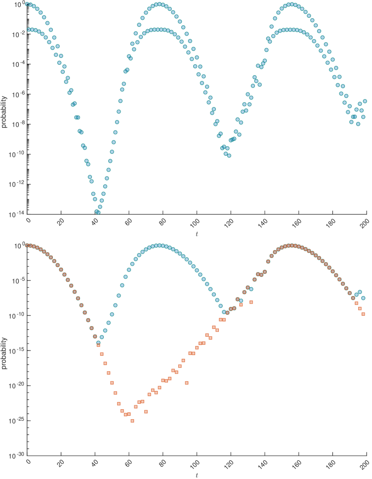
Figure 1: Illustration of the probabilities $\max_{x}P(x,t)$ and $P(0^{50},t)$ for a quantum walk on the 50-dimensional hypercube.
Upper panel. The maximum probability amongst all vertices $\max_{x}P(x,t)$.
Lower panel. Only even steps are shown. The circular markers: the maximum probability amongst all vertices $\max_{x}P(x,t)$ (same as in the upper panel for even $t$). The square markers: the probability at the initial vertex, $P(0^{50},t)$.
The data that support the graphs of this figure are available in the Zenodo repository https://doi.org/10.5281/zenodo.5907185.

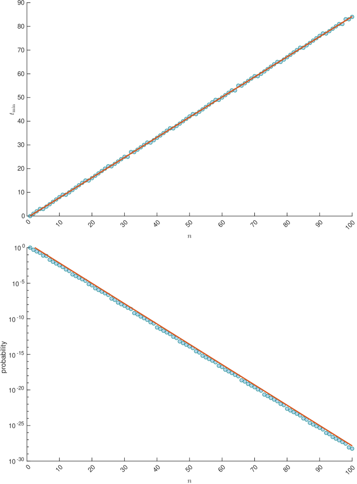
Figure 2: Illustration of $t_{\min}$ and $\max_{x}P(x,t_{\min})$ for various values of $n$.
Upper panel. The circular markers: the number of steps $t_{\min}$ to reach the minimum of $\max_{x}P(x,t)$. The solid line: the graph of the function $-0.754+0.849n$, which approximates $t_{\min}$.
Lower panel. The circular markers: the maximal (over all vertices of the hypercube) probability $\max_{x}P(x,t_{\min})$, at time $t_{\min}\approx 0.849n$. The solid line: the graph of the function $5\cdot 1.93^{-n}$, which is an upper bound on the probability.
The data that support the graphs of this figure are available in the Zenodo repository https://doi.org/10.5281/zenodo.5907185.

We note that $\max_{x}P(x,t)$ fluctuates between odd and even numbered steps, due to the walker being at an odd distance from the starting vertex $0^{n}$ after an odd number of steps and at an even distance from $0^{n}$ after an even number of steps. This effect is particularly pronounced when $\max_{x}P(x,t)$ is large. Then, a large fraction of the probability is concentrated on $0^{n}$ after even steps but, after odd steps, this probability is equally divided among $n$ vertices $x$ with $|x|=1$. As a result, the maximum $\max_{x}P(x,t)$ is visibly larger after an even number of steps. This effect becomes smaller when $\max_{x}P(x,t)$ is small.

The upper panel of Fig. 2 shows that the number of steps $t_{\min}$ required to minimize $\max_{x}P(x,t)$ grows linearly with $n$, and is achieved at approximately $-0.754+0.849n$. The probability $\max_{x}P(x,t_{\min})$ achieved at this $t_{\min}$ is approximately $5\cdot 1.93^{-n}$ (see the lower panel of Fig. 2).

Lastly, for $t\leq t_{\min}$ this maximum is achieved at $x=0^{n}$ (at even numbered steps) or at vertices $x$ with $|x|=1$ (for odd numbered steps). This is shown in the lower panel of Fig. 1 where we plot $\max_{x}P(x,t)$ and $P(0^{n},t)$ for even numbered steps $t$ (as the probability at $0^{n}$ is $0$ at odd steps). The panel shows that the maximum is achieved at $x=0^{n}$ until the moment when the probability $\max_{x}P(x,t)$ starts increasing again.

Rigorously, we can prove a weaker bound:

Theorem 1.

For any integer $t\in\left(0.86628n,0.86632n\right)$, we have $\max_{x}P(x,t)=O(1.4818^{-n})$.

Remark.

Even though we consider the case when the initial state is $\mathinner{\left\lvert\psi_{start}\right\rangle}$, the symmetry of the walk implies a similar result when starting in a state $\sum_{i=1}^{n}\frac{1}{\sqrt{n}}\mathinner{\left\lvert x,i\right\rangle}$, for any hypercube vertex $x$. This gives the following conclusion from Theorem 1: for all $x,y\in\{0,1\}^{n}$ and $t$ as in Theorem 1,

$$\frac{1}{n}\sum_{j=1}^{n}\left|\sum_{i=1}^{n}\mathinner{\left\langle y,j\right\rvert}W^{t}\mathinner{\left\lvert x,i\right\rangle}\right|^{2}=O(1.4818^{-n}).$$ (II.2)

III Proof of the main result

We first describe the strategy of the proof of Theorem 1. Because of the symmetry of the walk, all vertices $x$ with the same $|x|=k$ will have equal probabilities $P(x,t)$, see (III.5) below. Since there are ${\binom{n}{k}}$ vertices $x$, this immediately implies $P(x,t)\leq 1/{\binom{n}{k}}$. If $k$ is such that ${\binom{n}{k}}$ is sufficiently large, we get the desired upper bound on $P(x,t)$.

It remains to handle the case when ${\binom{n}{k}}$ is small. This corresponds to $k$ being either close to 0 ($0\leq k<0.13368n$) or close to $n$ ($(1-0.13368)n<k\leq n$). The second case is trivial: the number of time steps $t$ that we are considering is less than $(1-0.13368)n$, so, vertices $x$ with $|x|>(1-0.13368)n$ cannot be reached in $t$ steps.

For the first case, we show (Lemma 1) that if $P(x,t)$ is large, then $P(0^{n},t^{\prime})$ must also be non-negligible for some $t^{\prime}\in\{t-|x|,\ldots,t+|x|\}$. Therefore, one can show an upper bound on all $P(x,t)$ with $|x|\leq 0.13368n$ by upper bounding $P(0^{n},t^{\prime})$ for all $t^{\prime}:t-0.13368n\leq t^{\prime}\leq t+0.13368n$. This is done by Lemma 3 and Theorem 2, first expressing $P(0^{n},t^{\prime})$ in terms of Chebyshev polynomials and then bounding their asymptotics.

We begin by describing the evolution of the quantum walker in terms of states that utilize the symmetry of the walk. Denote

$$\mathinner{\left\lvert w,\rightarrow\right\rangle} =\frac{1}{\sqrt{{\binom{n}{w}}(n-w)}}\sum_{\begin{subarray}{c}x\\ |x|=w\end{subarray}}\sum_{\begin{subarray}{c}i\\ x_{i}=0\end{subarray}}\mathinner{\left\lvert x,i\right\rangle},$$ (III.1)

$$\mathinner{\left\lvert w,\leftarrow\right\rangle} =\frac{1}{\sqrt{{\binom{n}{w}}w}}\sum_{\begin{subarray}{c}x\\ |x|=w\end{subarray}}\sum_{\begin{subarray}{c}i\\ x_{i}=1\end{subarray}}\mathinner{\left\lvert x,i\right\rangle}.$$ (III.2)

By symmetry, the state of the quantum walk after any number of steps $t$ is of the form

$$\mathinner{\left\lvert\psi^{(t)}\right\rangle}=\sum_{w=0}^{n-1}\alpha^{(t)}_{w,\rightarrow}\mathinner{\left\lvert w,\rightarrow\right\rangle}+\sum_{w=1}^{n}\alpha^{(t)}_{w,\leftarrow}\mathinner{\left\lvert w,\leftarrow\right\rangle}.$$ (III.3)

Let

$$P[w,t]=|\alpha^{(t)}_{w,\rightarrow}|^{2}+|\alpha^{(t)}_{w,\leftarrow}|^{2}$$ (III.4)

be the total probability of the walker being at one of vertices $x$ with $|x|=w$ after $t$ steps. By the symmetry of the quantum walk,

$$P(x,t)=P[w,t]/{\binom{n}{w}}$$ (III.5)

for any $x:|x|=w$. In particular, $P(0^{n},t)=P[0,t]$.

III.1 Relating the probability to be at an arbitrary vertex with the probability to be at the initial vertex

The following Lemma shows that it suffices to bound $P[0,t^{\prime}]$ for a time interval $t^{\prime}\in[t-w^{\prime},t+w^{\prime}]$, as this would imply bounds on $P[w,t]$ for $w\leq w^{\prime}$.

Lemma 1.

Suppose that $n\geq 2$, $t\geq w^{\prime}$ and $P[0,t^{\prime}]\leq p_{0}$ for all $t^{\prime}\in[t-w^{\prime},t+w^{\prime}]$, where $w^{\prime}<n/2$. Then for all $w\in\{0,1,\ldots,w^{\prime}\}$, we have

$$P[w,t]\leq\frac{n^{w}}{w!}p_{0}.$$ (III.6)

Proof.

We prove the contrapositive: suppose that $P[w,t]=p_{w}$ for some $0<w<n/2$; then there exists a $t^{\prime}\in[t-w,t+w]$ such that $P[0,t^{\prime}]\geq\frac{w!p_{w}}{n^{w}}$.

We do this by showing two inequalities:

$$\max\left(|\alpha^{(t)}_{w,\leftarrow}|^{2},|\alpha^{(t+1)}_{w-1,\rightarrow}|^{2}\right)\geq\frac{w}{n-w}|\alpha^{(t)}_{w,\rightarrow}|^{2},$$ (III.7)

$$P[w-1,t-1]\geq|\alpha^{(t)}_{w,\leftarrow}|^{2}.$$ (III.8)

These two inequalities imply that one of $P[w-1,t-1],P[w-1,t+1]$ is at least

$$\min\left(\frac{w}{n-w}|\alpha^{(t)}_{w,\rightarrow}|^{2},|\alpha^{(t)}_{w,\leftarrow}|^{2}\right).$$ (III.9)

Because of (III.4), we must either have $|\alpha^{(t)}_{w,\rightarrow}|^{2}\geq\frac{n-w}{n}P[w,t]$ or $|\alpha^{(t)}_{w,\leftarrow}|^{2}\geq\frac{w}{n}P[w,t]$. In both cases (III.9) is at least $\frac{w}{n}P[w,t]$.

By repeating this argument $w$ times, we get that $P[0,t^{\prime}]$, for some $t^{\prime}\in[t-w,t+w]$ is at least

$$p_{w}\cdot\frac{w}{n}\cdot\frac{w-1}{n}\cdot\ldots\cdot\frac{1}{n}=\frac{w!\,p_{w}}{n^{w}}.$$ (III.10)

We now prove (III.7) and (III.8). To prove (III.7), consider vertices $x\in\{0,1\}^{n}$ for which $|x|=w$. Before the coin flip $D_{n}$, the amplitudes of $\mathinner{\left\lvert x,i\right\rangle}$ with $x_{i}=0$ are equal to $\frac{\alpha^{(t)}_{w,\rightarrow}}{\sqrt{(n-w){\binom{n}{w}}}}$ and the amplitudes of $\mathinner{\left\lvert x,i\right\rangle}$ with $x_{i}=1$ are equal to $\frac{\alpha^{(t)}_{w,\leftarrow}}{\sqrt{w{\binom{n}{w}}}}$. After applying the coin flip $D_{n}$, the amplitudes of $\mathinner{\left\lvert x,i\right\rangle}$ with $x_{i}=1$ become equal to

$$\frac{2(n-w)}{n}\frac{\alpha^{(t)}_{w,\rightarrow}}{\sqrt{(n-w){\binom{n}{w}}}}-\frac{n-2w}{n}\frac{\alpha^{(t)}_{w,\leftarrow}}{\sqrt{w{\binom{n}{w}}}}.$$ (III.11)

After the shift operation, each of those becomes an amplitude of $\mathinner{\left\lvert y,i\right\rangle}$ with $|y|=w-1$ and $y_{i}=0$. Since $\mathinner{\left\lvert w-1,\rightarrow\right\rangle}$ consists of ${\binom{n}{w}-1}(n-w+1)={\binom{n}{w}}w$ such $\mathinner{\left\lvert y,i\right\rangle}$, we have

$$\alpha^{(t+1)}_{w-1,\rightarrow}=\frac{2\sqrt{w(n-w)}}{n}\alpha^{(t)}_{w,\rightarrow}-\frac{n-2w}{n}\alpha^{(t)}_{w,\leftarrow}.$$ (III.12)

Assume that $|\alpha^{(t)}_{w,\leftarrow}|<\frac{\sqrt{w}}{\sqrt{n-w}}|\alpha^{(t)}_{w,\rightarrow}|$. (Otherwise, (III.7) is immediately true.) Then,

$$|\alpha^{(t+1)}_{w-1,\rightarrow}|\geq\left(\frac{2\sqrt{w(n-w)}}{n}-\frac{\sqrt{w}}{\sqrt{n-w}}\frac{n-2w}{n}\right)|\alpha^{(t)}_{w,\rightarrow}|.$$ (III.13)

The equation (III.7) now follows from

$$\frac{2\sqrt{w(n-w)}}{n}-\frac{\sqrt{w}}{\sqrt{n-w}}\frac{n-2w}{n}=\frac{\sqrt{w}}{\sqrt{n-w}}.$$ (III.14)

To prove (III.8), we simply note that $S\mathinner{\left\lvert w-1,\rightarrow\right\rangle}=\mathinner{\left\lvert w,\leftarrow\right\rangle}$. Since coin flip $D_{n}$ moves the amplitudes between $\mathinner{\left\lvert w-1,\leftarrow\right\rangle}$ and $\mathinner{\left\lvert w-1,\rightarrow\right\rangle}$, (III.8) expresses the fact that all the amplitude at $\mathinner{\left\lvert w,\leftarrow\right\rangle}$ after $t$ steps must have been at $\mathinner{\left\lvert w-1,\leftarrow\right\rangle}$ or $\mathinner{\left\lvert w-1,\rightarrow\right\rangle}$ one step earlier. This fact is obviously true. ∎

III.2 Bounding the probability to be at the initial vertex

Previously we demonstrated how the probability at a hypercube vertex is related to the probability at the initial vertex $P[0,t]$. Now we derive an explicit expression of $P[0,t]$ and apply it to upper-bound this probability.

In more details, we express (the square root of) the probability $P[0,t]$ through Chebyshev polynomials, see (III.28); then we apply an integral representation of Chebyshev polynomials (Lemma 2), arriving at an integral representation of the probability $P[0,t]$ (Eq. III.19).

The latter representation involving the integral $\int_{0}^{\infty}x^{-1}J_{t}(x)\cos(xz)\,\mathrm{d}x$ turns out far more suitable (compared to the expression involving Chebyshev’s polynomials) for proving an upper bound.

This is in part due to a clear separation between the oscillating part ($J_{t}$) and the exponential part ($\cos^{n}(x/n)$). This distinction helps to explain how the ratio $t/n$ leads to the oscillating behavior of $P[0,t]$ observed in the lower panel of Fig. 1 (with $n=50$). To illustrate this, examine the interplay between both parts in Fig. 3, for $n=50$ and different values of $t$.

• When $t/n$ is “small” (e.g., see the upper row in Fig. 3 with $n=50$, $t=0.12n$), the Bessel function’s first maximum largely overlaps with the contribution of $\cos^{n}(\cdot)$ in the vicinity of $x=0$. However, the subsequent maxima of $\cos^{n}(\cdot)$ occur where the oscillations of $J_{t}$ cancel out, resulting in an insignificant contribution to the integral. Therefore, the value of the integral is dominated by the values of the integrand near $x=0$ and the probability $P[0,t]$ is large.

• Now consider the case when $t/n$ is “large” (see the middle row in Fig. 3 for the case $n=50$, $t=3.12n$). While the Bessel function’s values near $x=0$ are negligible, the following local maximum greatly overlaps with the next peak of $\cos^{n}(x/n)$ (in the vicinity of $x\approx\pi n$). This results in a large contribution to the integral, which is not canceled out by the following peaks of $\cos^{n}(x/n)$ (where the Bessel function’s fluctuations make the contribution to the integral negligible).

• Finally, when $t/n$ is “just right” (see the lower row in Fig. 3 for the case $n=50$, $t=0.84n$), the first maxima of the Bessel function occur when $\cos^{n}(x/n)$ is near zero. This ensures that the resulting integrand’s oscillations near each peak of $\cos^{n}(x/n)$ largely cancel out. We proceed to quantify the remaining integral’s value and show that it indeed is exponentially small in $n$.

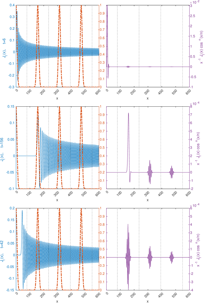
Figure 3: Illustration of the integrand and its factors for $n=50$ and $t=0.12n$ (upper row), $t=3.12n$ (middle row), $t=0.84n$ (lower row). Panels on the left show $J_{t}(x)$, solid line, with units on the left axis and $\cos^{n}(x/n)$, dash-dotted line, with units on the right axis. Panels on the right depict the integrand $x^{-1}J_{t}(x)\cos^{n}\frac{x}{n}$. The dotted gridlines divide the real line into subintervals separating the peaks of $\cos^{n}(x/n)$.

Despite this intuition, at first glance both expressions of $\sqrt{P[0,t]}$ (the discrete sum involving Chebyshev polynomials and the integral) suffer the same drawback (or the advantage) of catastrophic cancellations. Indeed, while the integrand’s extreme values near each peak of $\cos^{n}(x/n)$ are polynomially decaying in $n$, cancellations ensure that the overall contribution is exponentially small! This property prohibits from making simple estimates of $\sqrt{P[0,t]}$ in either case. However, here the main advantage of the integral representation manifests itself: instead of computing integrals over real intervals, we can exploit Cauchy’s integral theorem to transform them to contour integrals in the complex plane. Since the integrand turns out to be non-oscillatory in the complex plane in directions orthogonal to the real axis, this provides an efficient way to estimate the value of $P[0,t]$. This approach leads to the asymptotic estimates in Theorem 2 and the desired upper bound on the probability $P[0,t]$.

The rigorous arguments begin with a proof of the following representation of Chebyshev polynomials of even order, valid for $|z|\leq 1$:

Lemma 2.

Let $t$ be a positive even integer; then the following equality is valid for all $z\in[-1,1]$:

$$T_{t}(z)=(-1)^{t/2}\,t\int_{0}^{\infty}x^{-1}J_{t}(x)\cos(xz)\,\mathrm{d}x,$$ (III.15)

where $T_{t}$ is the $t^{\text{th}}$-degree Chebyshev polynomial of the first kind and $J_{t}$ stands for the Bessel function of the first kind.

Proof.

We start with a special case of the Sonine-Schafheitlin formula(Watson, 1922, p.405, §13.42, Eq. (3))

$$\int_{0}^{\infty}\frac{J_{\mu}(ax)\cos(bx)}{x}\,\mathrm{d}x=\mu^{-1}\cos\left(\mu\arcsin(b/a)\right),\quad 0<b\leq a.$$ (III.16)

Taking $a=1$, $b=z\in(0,1]$ and $\mu=t$ in (III.16) gives

$$\int_{0}^{\infty}\frac{J_{t}(x)\cos(x\,z)}{x}\,\mathrm{d}x =\frac{\cos\left(t\cdot\arcsin z\right)}{t}.$$ (III.17)

It remains to notice that

$$\cos\left(t\cdot\arcsin z\right)=\cos\left(t\left(\frac{\pi}{2}-\arccos z\right)\right)=(-1)^{t/2}\cos(t\arccos{z})=(-1)^{t/2}T_{t}(z).$$ (III.18)

Continuity and evenness of $\cos$ and $T_{t}$ ensures the validity of (III.15) for $z\in[-1,0]$. ∎

The following Lemma allows us to characterize the probability $P[0,t]$ to obtain the vertex $0^{n}$ after $t$ steps as follows:

Lemma 3.

Let $t$ be a positive integer; if $t$ is odd, then $P[0,t]=0$. If $t$ is even, then

$$\sqrt{P[0,t]}=\frac{1}{2^{n}}\sum_{m=0}^{n}\binom{n}{m}T_{t}\left(1-\frac{2m}{n}\right)=t\left|\int_{0}^{\infty}x^{-1}J_{t}(x)\cos^{n}\frac{x}{n}\,\mathrm{d}x\right|\,.$$ (III.19)

Proof.

Due to the symmetry of the walk (w.r.t. permuting the coordinates of the hypercube), the amplitudes of $\mathinner{\left\lvert 0^{n},j\right\rangle}$ for all $j\in[n]$ remain equal after any number of steps. Therefore,

$$P[0,t]=\langle\psi_{start}|W^{t}|\psi_{start}\rangle^{2}.$$ (III.20)

Let $\mathinner{\left\lvert v_{j}\right\rangle}$ be the eigenvectors of $W$, with eigenvalues $\mathrm{e}^{\mathrm{i}\lambda_{j}}$. We can represent $\mathinner{\left\lvert\psi_{start}\right\rangle}$ as a linear combination of the eigenvectors, $\mathinner{\left\lvert\psi_{start}\right\rangle}=\sum_{j}a_{j}\mathinner{\left\lvert v_{j}\right\rangle}$, then

$$\sqrt{P[0,t]}=\langle\psi_{start}|W^{t}|\psi_{start}\rangle=\sum_{j}|a_{j}|^{2}\mathrm{e}^{\mathrm{i}t\lambda_{j}}.$$ (III.21)

As described in Moore and Russell (2002), $W$ has $2^{n+1}$ eigenvectors that have non-zero overlap with the starting state. These eigenvectors can be indexed by $k\in\{0,1\}^{n}$. For each $k\in\{0,1\}^{n}$, we have a pair of eigenvectors $\mathinner{\left\lvert v^{+}_{k}\right\rangle}$ and $\mathinner{\left\lvert v^{-}_{k}\right\rangle}$ with eigenvalues $\mathrm{e}^{\pm\mathrm{i}w_{m}}$ where $m=|k|$ is the Hamming weight of $k$ and $w_{m}$ is such that $\cos w_{m}=1-{2m}/{n}$. Furthermore, all of those eigenvectors have equal overlap with the starting state: $|\langle v^{+}_{k}\mathinner{\left\lvert\psi_{start}\right\rangle}|^{2}=|\langle v^{-}_{k}\mathinner{\left\lvert\psi_{start}\right\rangle}|^{2}=\frac{1}{2^{n+1}}$. Therefore, we get

$$\sqrt{P[0,t]} =\frac{1}{2^{n+1}}\sum_{k\in\{0,1\}^{n}}\left(\mathrm{e}^{\mathrm{i}tw_{m}}+\mathrm{e}^{-\mathrm{i}tw_{m}}\right)$$ (III.22)

$$=\frac{1}{2^{n}}\sum_{k\in\{0,1\}^{n}}\cos w_{m}t$$ (III.23)

$$=\frac{1}{2^{n}}\sum_{m=0}^{n}\binom{n}{m}\cos w_{m}t$$ (III.24)

$$=\frac{1}{2^{n}}\sum_{m=0}^{n}\binom{n}{m}\cos\left(t\cdot\arccos\left(1-2\cdot\frac{m}{n}\right)\right)$$ (III.25)

$$=\frac{1}{2^{n}}\sum_{m=0}^{n}\binom{n}{m}T_{t}\left(1-2\cdot\frac{m}{n}\right).$$ (III.26)

If $t$ is odd, then so is $T_{t}$ and the terms in (III.26) cancel out; otherwise, using (III.15) with $z=(n-2m)/n$ for even integer $t$,

$$\frac{1}{2^{n}}\sum_{m=0}^{n}\binom{n}{m}T_{t}\left(1-\frac{2m}{n}\right) =(-1)^{t/2}t\int_{0}^{\infty}x^{-1}J_{t}(x)\sum_{m=0}^{n}\frac{1}{2^{n}}\binom{n}{m}\cos\left(x-\frac{2x\,m}{n}\right)\,\mathrm{d}x$$ (III.27)

$$=(-1)^{t/2}t\int_{0}^{\infty}x^{-1}J_{t}(x)\cos^{n}\frac{x}{n}\,\mathrm{d}x$$ (III.28)

with the last step following from the binomial expansion of $(\mathrm{e}^{\mathrm{i}x/n}+\mathrm{e}^{-\mathrm{i}x/n})^{n}$. ∎

The most technical contribution of this manuscript is an upper bound of the integral appearing in Lemma 3, provided that $t/n$ is suitably bounded. In what follows, we use $\nu\in\mathbb{R}$ instead of $t$ (since the latter was assumed to be an even integer in our notation before).

Theorem 2.

Denote $a_{k}=(k-0.5)\pi$, $k=1,2,3,\ldots$; let a positive constant $\alpha\in(\frac{\pi}{6},1)$ be fixed.

For $n\geq 2$ and $\nu>1$, satisfying $\nu\in(n\alpha,n)\subset\left(\frac{\pi n}{6},n\right)$, the following estimates hold:

The tail: $$\left|\int_{na_{n}}^{\infty}x^{-1}J_{\nu}(x)\cos^{n}\left(\frac{x}{n}\right)\,\mathrm{d}x\right|<\frac{100\sqrt{n}}{2^{n}};$$ (III.29)

The middle part: $$\left|\int_{na_{1}}^{na_{n}}x^{-1}J_{\nu}(x)\cos^{n}\left(\frac{x}{n}\right)\,\mathrm{d}x\right|<\frac{4000\sqrt{n}}{1.541^{n}};$$ (III.30)

The bulk: $$\left|\int_{0}^{na_{1}}x^{-1}J_{\nu}(x)\cos^{n}\left(\frac{x}{n}\right)\,\mathrm{d}x\right|<\frac{3}{(1+\alpha)^{0.5\alpha n}}.$$ (III.31)

The proof of the Theorem is deferred to Appendix A; below we roughly sketch a reasoning behind the proof.

As Fig. 3 might suggest, it is advantageous to divide the whole integral into a sum of integrals over subintervals of the form ${[(k-0.5)\pi n,(k+0.5)\pi n]}$, separating the individual peaks of $\cos^{n}(x/n)$ and estimating the contribution of each integral separately. It turns out that there are three regimes to consider:

1. When $k\geq n$, the integral over each subinterval $[(k-0.5)\pi n,(k+0.5)\pi n]$ turns out to be of order $2^{-n}n^{1/2}k^{-5/2}$; the series (taking the sum over $k:k\geq n$) converges, leading to the tail estimate (III.29).

2. When $1\leq k<n$, we estimate the integral over each subinterval $[(k-0.5)\pi n,(k+0.5)\pi n]$ as $1.541^{-n}n^{-1/2}$, with the constant $1.541$ coming from an upper bound on a certain auxiliary function. Since there are $n-1$ such subintervals, this leads to the estimate of the middle part (III.30).

3. In both previous cases, the integral is going to be estimated via an excursion into the complex plane. However, for the remaining interval $(0,0.5\pi n)$ this is not a viable option anymore. Instead, here we combine direct bounds on the Bessel function $J_{\nu}$ and the $\cos^{n}(x/n)$ term when $x$ is “small”. These estimates (in particular, the estimate of the integral over the interval $[0,\nu]$) lead to the dominating contribution (“the bulk”) (III.31).

To estimate the integrals of the form $\int_{na_{k}}^{na_{k+1}}x^{-1}J_{\nu}(x)\cos^{n}\left(\frac{x}{n}\right)\,\mathrm{d}x$, we form a rectangle in the complex plane, consisting of the real interval ${[na_{k},na_{k+1}]}$, a parallel interval ${[na_{k}+\mathrm{i}R,na_{k+1}+\mathrm{i}R]}$ for some $R>0$, as well as two segments orthogonal to the real axis forming a closed contour. The Cauchy integral theorem then implies that the integral over the real integral coincides with the integral over the rest of the contour. While the integrand still is oscillatory over the set ${[na_{k}+\mathrm{i}R,na_{k+1}+\mathrm{i}R]}$, its absolute value vanishes as $R\to+\infty$. Thus, taking the limit $R\to+\infty$, we are left with integrals over the rays of the form $[na_{k},na_{k}+\mathrm{i}\infty)$.

For this strategy to work, we need the integrand to be holomorphic (in a domain containing the integration contour). We note that the integrand $x^{-1}J_{\nu}(x)\cos^{n}\left(\frac{x}{n}\right)$ is the real part of the function

$$f(z)=\frac{H^{(1)}_{\nu}(z)\cos^{n}(z/n)}{z},\quad z\in\mathbb{C},\ \left|z\right|>1,$$ (III.32)

where $H^{(1)}_{\nu}$ is the Hankel function of the first kind (and satisfies $\Re H^{(1)}_{\nu}(x)=J_{\nu}(x)$ for real $x$). Now $f$ is holomorphic in the necessary domain, and we make use of the estimate

$$\left|\int_{na_{k}}^{na_{k+1}}x^{-1}J_{\nu}(x)\cos^{n}\left(\frac{x}{n}\right)\,\mathrm{d}x\right|=\left|\Re\int_{na_{k}}^{na_{k+1}}f(x)\,\mathrm{d}x\right|\leq\left|\int_{na_{k}}^{na_{k+1}}f(x)\,\mathrm{d}x\right|.$$ (III.33)

Finally, to bound the values of $f$ on the rays $[na_{k},na_{k}+\mathrm{i}\infty)$, we will employ asymptotic expansions of the Hankel function $H^{(1)}_{\nu}(z)$. The case of large $z$ is straightforward (DLMF, , §10.17(iv)). However, when the argument $z$ and order $\nu$ are of similar magnitude, there is no suitable expansion of the Hankel function with error bounds (to the best of our knowledge). This leads to the most involved argument in this paper, where we relate the Hankel function to the modified Bessel function of the second kind, then consider its asymptotic expansion and bound the relevant error term, as detailed in Section A.6.

III.3 Concluding the proof

Finally, we are ready to show Theorem 1. As explained at the beginning of Section III, the overall strategy for bounding $P(x,t)$ is to consider two cases, depending on the Hamming weight of the vertex $x$. Now we sketch an informal outline of the remaining argument.

Let $c<0.5$ be a constant (its value to be determined); consider two cases: when $\left|x\right|$ is between $cn$ and $(1-c)n$ (then the binomial coefficient $\binom{n}{\left|x\right|}$ is “large”) and when $\left|x\right|<cn$ (then the vertex $x$ is “close” to the initial vertex). We also set $t=(1-c)n$ (thus the case $\left|x\right|>(1-c)n$ need not be considered) and $\alpha=(1-2c)$ (the constant appearing in Theorem 2).

1. In the former case, we apply $P(x,t)\leq 1/{\binom{n}{\left|x\right|}}\leq 1/{\binom{n}{{cn}}}$. The latter quantity is (roughly; for a precise statement, see (III.44)) bounded by

   $$2^{-H(c)n}=\left(c^{c}(1-c)^{(1-c)}\right)^{n}.$$ (III.34)

2. In the latter case, we rely on the already proven relationship between $P(x,t)$ and $P(0^{n},t^{\prime})$ for some $t^{\prime}\in[t-cn,t+cn]\subset[(1-2c)n,n]$; specifically, we apply Lemmas 1 and 3 and intend to upper-bound the integral via (III.31) (which is the dominating term) with $\alpha=(1-2c)$. This (again, roughly; the precise statement is (III.43)) leads to the following upper bound on $P(x,t)$:

   $$\left(\frac{\mathrm{e}(1-c)^{1-c}}{(2-2c)^{(1-2c)}}\right)^{n}=\left(\frac{\mathrm{e}(1-c)^{c}}{2^{(1-2c)}}\right)^{n}.$$ (III.35)

Now by balancing the estimates (III.34) and (III.35), we obtain the equilibrium value $c=0.133682\ldots$. However, the above reasoning is faulty: it ignores the fact that Theorem 2 requires $t^{\prime}$ to be within the open set $(\alpha n,n)$. Also, $1/{\binom{n}{{cn}}}$ is, in fact, not upper-bounded by $2^{-H(c)n}$ (a polynomial factor is missing). To fix these issues, we choose slightly smaller values of $\alpha$ and $t$, leading to a slightly worse overall estimate.

This leads to the following proof of Theorem 1 (restated here for convenience). See 1

Proof.

We assume that $n$ is sufficiently large, i.e., $\left(0.86628n,0.86632n\right)\cap\mathbb{Z}\neq\emptyset$ and $n>\max\{n_{0},1\}$, where $n_{0}$ is described below. Let $t$ be from the indicated range; set $w^{\prime}=0.13368n$ and $\alpha=0.7326$ in Theorem 2. The chosen constants ensure that $[t-w^{\prime},t+w^{\prime}]\subset(0.7326n,n)$.

Then $(1+\alpha)^{0.5\alpha}>1.22302$ and Theorem 2 gives the estimate (for $t^{\prime}\in(\alpha n,n)$)

$$\left|\int_{0}^{\infty}x^{-1}J_{t^{\prime}}(x)\cos^{n}\left(\frac{x}{n}\right)\,\mathrm{d}x\right|<\frac{100\sqrt{n}}{2^{n}}+\frac{4000\sqrt{n}}{1.541^{n}}+\frac{3}{1.22302^{n}}=O\left(1.22302^{-n}\right).$$ (III.36)

This together with Lemma 3 implies that there are positive constants $C_{0},C_{1}$ and a positive integer $n_{0}$ such that for all $n>n_{0}$ and all $t^{\prime}\in(\alpha n,n)=(0.7326n,n)$ the probability $P[0,t^{\prime}]$ can be estimated as

$$P[0,t^{\prime}]<\frac{C_{0}n{t^{\prime}}^{2}}{1.22302^{2n}}\leq\frac{C_{0}n^{3}}{1.49578\ldots^{n}}<\frac{C_{1}}{1.49578^{n}},\quad t^{\prime}\in(0.7326n,n).$$ (III.37)

In particular,

$$P[0,t^{\prime}]<\frac{C_{1}}{1.49578^{n}}\quad\text{for all }t^{\prime}\in[t-w^{\prime},t+w^{\prime}]\subset(0.7326n,n).$$ (III.38)

Fix any $x\in\{0,1\}^{n}$ and let $w=|x|$. If $w>n-w^{\prime}>t$, then the discrete-time quantum walk cannot reach $x$ in $t$ steps, thus $P(x,t)=0$. Therefore there are two possibilities to consider:

1. $w\leq w^{\prime}$, then Eq. III.5 and Lemma 1 with $p_{0}=C_{1}\cdot 1.49578^{-n}$ give

   $$P(x,t)=\frac{P[w,t]}{\binom{n}{w}}\leq p_{0}\frac{n^{w}(n-w)!}{n!}<\frac{C_{1}}{1.49578^{n}}\cdot n^{nc}\cdot\frac{(n-nc)!}{n!}$$ (III.39)

   with $c:=w^{\prime}/n=0.13368$. Lower and upper bounds Robbins (1955) on the factorials yield

   $$n!\geq\left(\frac{n}{\mathrm{e}}\right)^{n}\mathrm{e}^{\frac{1}{12n+1}}\sqrt{2\pi n}\,\text{ and }\,(n-nc)!\leq\left(\frac{n(1-c)}{\mathrm{e}}\right)^{n(1-c)}\mathrm{e}^{\frac{1}{12n(1-c)}}\sqrt{2\pi n(1-c)},$$ (III.40)

   leading to

   $$\frac{(n-nc)!}{n!}\leq\left(\frac{n^{(1-c)}(1-c)^{(1-c)}\cdot\mathrm{e}}{\mathrm{e}^{(1-c)}\cdot n}\right)^{n}\mathrm{e}^{\frac{1}{12n(1-c)}-\frac{1}{12n+1}}\sqrt{(1-c)}.$$ (III.41)

   Now, since $\mathrm{e}^{\frac{1}{12n(1-c)}-\frac{1}{12n+1}}<\mathrm{e}^{\frac{1}{12(1-c)}}<2$ and $\sqrt{(1-c)}<1$, we have

   $$\frac{(n-nc)!}{n!}<2n^{-nc}\mathrm{e}^{nc}(1-c)^{(1-c)n}<2\cdot 0.99068^{-n}n^{-nc},$$ (III.42)

   because $\mathrm{e}^{c}(1-c)^{(1-c)}=0.990681\ldots^{-1}<0.99068^{-1}$. Let $C_{2}=2C_{1}$, then we conclude

   $$P(x,t)<\frac{C_{2}}{(1.49578\cdot 0.99068)^{n}}<\frac{C_{2}}{1.4818^{n}}=O\left(1.4818^{-n}\right).$$ (III.43)

2. $w^{\prime}<w\leq n-w^{\prime}$, then (III.5) and a lower bound (Mitzenmacher and Upfal, 2005, Lemma 9.2) on the binomial coefficient in terms of the binary entropy function $H$ gives

   $$P(x,t)\leq\binom{n}{w^{\prime}}^{-1}\leq(n+1)2^{-nH(w^{\prime}/n)}=(n+1)\left(2^{H(0.13368)}\right)^{-n}.$$ (III.44)

   Since $2^{H(0.13368)}=1.48189\ldots$, we arrive at $P(x,t)=(n+1)\cdot 1.48189\ldots^{-n}=O(1.4818^{-n})$.

∎

IV Summary and outlook

We have shown that quantum walk on the hypercube quickly disperses over vertices so well that no vertex has more than an exponentially small part of the quantum state on it. This dispersion property is significantly stronger than the standard mixing property which requires that the walk has spread almost uniformly over the vertices but allows significant spikes on particular vertices.

Our computer simulations show that, after $O(n)$ steps of the standard discrete time quantum walk on a $n$-dimensional hypercube, the probability of being at any vertex of the hypercube is at most $1.93...^{-n}$. Since the $n$-dimensional hypercube has $2^{n}$ vertices, this dispersion is close to the maximum possible. While there is a number of results about fast mixing of quantum walks Levin and Peres (2017); Randall (2006), such strong dispersion results have been rare. Rigorously, we can show that the probability of the walker being at any vertex is $1.4818...^{-n}$. The proof uses an intricate argument about asymptotics of Bessel and Hankel functions.

All of those results are for a starting state where the walker is localized in one vertex of the hypercube and the initial direction for the walker is the uniform superposition of all $n$ possible directions. For the case when the initial direction of the walker is a basis state corresponding to one direction, the quantum walk shows an oscillatory localization, with a large fraction of the walker’s state staying either in the starting vertex or its neighbouring vertex, depending on the step of the walk Ambainis et al. (2016).

A particular application of our results would be to show an exponential advantage for quantum algorithms in the query model for the case when the main non-query transformation is a quantum walk, along the lines of Brandão and Horodecki (2013); Aaronson and Ambainis (2018). A technical difficulty here is that the dispersion result only holds for starting states where the direction register of the walker is in the uniform superposition. Thus, proving an exponential advantage requires generalizing the conditions from Brandão and Horodecki (2013) for achieving an exponential advantage, which is a subject of future work.

Appendix A Bounding the integral

A.1 Preliminaries

Throughout the proof, we will make use of standard notation of some special functions; $\Gamma$ will stand for the gamma function; $B$ denotes the beta function, satisfying $B(x,y)=\Gamma(x)\Gamma(y)/\Gamma(x,y)$. The Bessel functions of the first and second kind will be denoted as $J_{\nu}(x)$ and $Y_{\nu}(x)$, respectively; and the Hankel function of the first kind is denoted as $H^{(1)}_{\nu}(x)=J_{\nu}(x)+\mathrm{i}Y_{\nu}(x)$. As in the statement of the Theorem, we denote $a_{k}=(k-0.5)\pi$, $k=1,2,3,\ldots$, and let a positive constant $\alpha\in(\frac{\pi}{6},1)$ be fixed. Furthermore, let $\nu>0$ and suppose an integer $n\geq 2$ satisfies

$$n\geq\frac{1}{\alpha}\quad\text{and}\quad\alpha<\frac{\nu}{n}<1.$$

Also, for $a,b\in\mathbb{R}$, with $a<b$, we define $D_{a,b}=\left\{x+\mathrm{i}y\ \vline\ x\in[a,b],\ 0\leq y<\infty\right\}$ (i.e., $D_{a,b}$ stands for an “infinite rectangle” in the complex plane with one side being the real interval $[a;b]$).

A.2 Asymptotic expansions of the Hankel function

The case of large argument.

When $z\in\mathbb{C}$, $\left|\arg z\right|\in[0,\pi-\delta)$ for an arbitrary small positive constant $\delta$, we have (DLMF, , §10.17(iv))

$$H^{(1)}_{\nu}(z)=\sqrt{\frac{2}{\pi z}}\,\mathrm{e}^{\mathrm{i}(z-\nu\pi/2-\pi/4)}\left(1+\rho(\nu,z)\right),$$ (A.1)

where the principal branch of $\sqrt{z}$ is used, and

$$\left|\rho(\nu,z)\right|\leq\left(\nu^{2}-1/4\right)\left|z\right|^{-1}\exp\left(\left(\nu^{2}-1/4\right)\left|z\right|^{-1}\right).$$ (A.2)

For future reference, we note that whenever $z$ additionally satisfies $\left|z\right|\geq n^{2}$, we have (since $\nu<n$)

$$\left|\rho(\nu,z)\right|<\nu^{2}\left|z\right|^{-1}\exp\left(\nu^{2}\left|z\right|^{-1}\right)<\mathrm{e}$$ (A.3)

and

$$\left|H^{(1)}_{\nu}(z)\right|\leq\sqrt{\frac{2}{\pi}}\left(1+\mathrm{e}\right)\left|\mathrm{e}^{\mathrm{i}z}\right|\left|z\right|^{-1/2}<\frac{3\mathrm{e}^{-\Im(z)}}{\left|z\right|^{1/2}}.$$ (A.4)

The case when argument and order are of similar magnitude.

Lemma 4.

When $\arg w\in[0;\pi/2)$ and $\Re w>1$, we have

$$H^{(1)}_{\nu}(\nu w)=-\mathrm{i}\,\sqrt{\frac{2}{\pi\nu}}\,\frac{\mathrm{e}^{\mathrm{i}\nu(\sqrt{w^{2}-1}-\arccos(1/w))}}{(1-w^{2})^{0.25}}\left(1+\eta(\nu,-\mathrm{i}w)\right),$$ (A.5)

where the fractional powers and the logarithm take their principal values on the positive real axis and the term $\eta$ can be bounded as

$$\left|\eta(\nu,-\mathrm{i}w)\right|\leq\exp\left(\frac{2\mathcal{V}_{+\infty,-\mathrm{i}w}}{\nu}\right)\,\frac{2\mathcal{V}_{+\infty,-\mathrm{i}w}}{\nu},$$

and the quantity $\mathcal{V}_{+\infty,-\mathrm{i}w}$ satisfies

$$\mathcal{V}_{+\infty,-\mathrm{i}w}\leq\frac{1}{12}+\frac{1}{6\sqrt{5}}+\left(\frac{4}{27}\right)^{1/4}+\frac{c^{2}(c^{2}+2)}{\sqrt{8}(c^{2}-1)^{2.5}},\qquad c:=\Re w>1,\ \Im w\geq 0.$$

Moreover, when $\nu\geq 1$ and $w\in\mathbb{C}$ satisfies $\Re(w)\geq\pi/2$ and $\Im(w)\geq 0$, we have

$$\left|1+\eta(\nu,-\mathrm{i}w)\right|\leq 430.$$ (A.6)

The proof is postponed until Section A.6.

A.3 Auxiliary lemmata

Here we list a few somewhat disjoint auxiliary results that will be useful in the subsequent analysis.

Lemma 5.

Suppose that $f:D\to\mathbb{C}$ is holomorphic in $D$, where $D$ is a domain containing the region $D_{a,b}:=\left\{x+\mathrm{i}y\ \vline\ x\in[a,b],\ 0\leq y<\infty\right\}$, for some reals $a<b$. Moreover, assume that

1. $\lim\limits_{R\to+\infty}\sup_{x\in[a,b]}\left|f(x+\mathrm{i}R)\right|=0$, and

2. integrals $\int_{0}^{\infty}f(a+\mathrm{i}y)\,\mathrm{d}y$, $\int_{0}^{\infty}f(b+\mathrm{i}y)\,\mathrm{d}y$ converge.

Then

$$\int_{a}^{b}f(x)\,\mathrm{d}x=\mathrm{i}\int_{0}^{\infty}\left(f(a+\mathrm{i}y)-f(b+\mathrm{i}y)\right)\,\mathrm{d}y.$$ (A.7)

Proof.

For every $R>0$ consider the positively oriented rectifiable curve $\gamma_{R}$ consisting of the line segments

$$[a,b]\cup\left\{b+\mathrm{i}y\ \vline\ y\in[0,R]\right\}\cup\left\{x+\mathrm{i}R\ \vline\ x\in[a,b]\right\}\cup\left\{a+\mathrm{i}y\ \vline\ y\in[0,R]\right\}.$$

By Cauchy’s integral theorem we have $\oint_{\gamma_{R}}f(z)\,\mathrm{d}z=0$, i.e.,

$$\int_{a}^{b}f(x)\,\mathrm{d}x+\mathrm{i}\int_{0}^{R}f(b+\mathrm{i}y)\,\mathrm{d}y-\int_{a}^{b}f(x+\mathrm{i}R)\,\mathrm{d}x-\mathrm{i}\int_{0}^{R}f(a+\mathrm{i}y)\,\mathrm{d}y=0.$$

Rearrange this equality as

$$\int_{a}^{b}f(x)\,\mathrm{d}x=\mathrm{i}\left(\int_{0}^{R}f(a+\mathrm{i}y)\,\mathrm{d}y-\int_{0}^{R}f(b+\mathrm{i}y)\,\mathrm{d}y\right)+\int_{a}^{b}f(x+\mathrm{i}R)\,\mathrm{d}x$$

and take the $R\to\infty$ limit. Since

$$\left|\int_{a}^{b}f(x+\mathrm{i}R)\,\mathrm{d}x\right|\leq(b-a)\sup_{x\in[a,b]}\left|f(x+\mathrm{i}R)\right|,$$

which tends to 0 by the assumptions of $f$, we are done. ∎

Lemma 6.

For all $a>0$ the following equalities hold:

$$\int_{0}^{\infty}\frac{\,\mathrm{d}y}{(a^{2}+y^{2})^{3/4}}=\frac{B(0.5,0.25)}{2\sqrt{a}}\approx 2.62206\ldots\cdot a^{-0.5},$$ (A.8)

$$\int_{0}^{\infty}\frac{\,\mathrm{d}y}{(a^{2}+y^{2})^{5/4}}=\frac{B(0.5,0.75)}{2\sqrt{a^{3}}}\approx 1.1984\ldots\cdot a^{-1.5}.$$ (A.9)

Proof.

The first equality can be proven as follows: substitute $t=a^{2}y^{2}$, which gives $\,\mathrm{d}y=0.5at^{-1/2}\,\,\mathrm{d}t$. Then

$$\int_{0}^{\infty}\frac{\,\mathrm{d}y}{(a^{2}+y^{2})^{3/4}}=\frac{a}{2}\cdot\frac{1}{a^{3/2}}\int_{0}^{\infty}\frac{t^{-1/2}\,\mathrm{d}t}{(1+t)^{3/4}}=\frac{1}{2a^{1/2}}\int_{0}^{\infty}\frac{t^{1/2-1}\,\mathrm{d}t}{(1+t)^{1/2+1/4}}.$$

Now from the identity $B(x,y)=\int_{0}^{\infty}\frac{t^{x-1}\,\mathrm{d}t}{(1+t)^{x+y}}$ we recognize the integral on the RHS as the beta function value $B(0.5,0.25)=\Gamma(0.5)\Gamma(0.25)/\Gamma(1.25)\approx 5.24412\ldots$. In a similar manner one shows the second equality. ∎

Lemma 7.

For all $t\in[0;\pi/2)$ the inequality $\cos t\leq\mathrm{e}^{-t^{2}/2}$ holds.

Proof.

Let $h(t)=\ln(\cos(t))+t^{2}/2$ and consider $h^{\prime}(t)=t-\tan(t)$. Since $h^{\prime}(0)=0$ and $h^{\prime}(t)<0$ for $t\in(0;\pi/2)$, $h$ attains its maximum at $t=0$, i.e., $\ln(\cos t)\leq-t^{2}/2$ with equality at $t=0$. Exponentiating gives the desired result. ∎

Lemma 8.

Let $g$ be defined in the set $\left\{z\in\mathbb{C}\ \vline\ \Re z\geq 1,\Im z\geq 0\right\}$ via

$$g(z)=z-\sqrt{z^{2}-1}+\arccos(1/z),$$

where the square root and the inverse cosine functions take their principal values on the positive real axis. Then $\Im(g(z))<0.2607$ for all $z$ with $\Re z\geq 1$, $\Im z\geq 0$.

Proof.

Let $R>0$; we will assume that $R$ is large enough, e.g., $R>1$.

Since $g$ is holomorphic on the domain $\left\{x+\mathrm{i}y\ \vline\ x\in(1,R),\ y\in(0,R)\right\}$ and continuous on its closure, its imaginary part $\Im(g(z))$ is harmonic and attains its maximum on the boundary of this region. Moreover, as $g(z)\in\mathbb{R}$ when $\Im z=0$ and

$$\lim\limits_{\left|z\right|\to\infty}\left|z-\sqrt{z^{2}-1}\right|=0\quad\text{and}\quad\lim\limits_{\left|z\right|\to\infty}\arccos(1/z)=\pi/2,$$

it follows that $\Im(g(z))$ must attain its maximum on the segment with $\Re z=1$, $\Im z\in[0,R]$.

Let us separate the real and imaginary part of $g$, i.e., introduce real-valued bivariate functions $u,v$ satisfying $g(x+\mathrm{i}y)=u(x,y)+\mathrm{i}v(x,y)$. By the arguments above, we need to show that $v(1,y)<0.2607$ for all $y\in[0,R]$, for arbitrarily large $R$. We will show that (for $R>1$) the function $v(1,\cdot)$ has a single local maximum at $y_{0}\approx 0.86883\ldots$ where its value is less than $0.2607$. To calculate the derivative of $y\mapsto v(1,y)$ and show that it is positive on $(0,y_{0})$ and negative on $(y_{0},R)$, we employ Cauchy-Riemann equations.

Consider the derivative of $g(z)$, denoted by $g^{(1)}(z)$:

$$g^{(1)}(z):=\frac{\,\mathrm{d}}{\,\mathrm{d}z}g(z)=1-\frac{z}{\sqrt{z^{2}-1}}+\frac{1}{z^{2}\sqrt{1-z^{-2}}}=1-\frac{\sqrt{z^{2}-1}}{z}.$$

Separate the real and imaginary parts of the derivative, i.e., $g^{(1)}(x+\mathrm{i}y)=u^{(1)}(x,y)+\mathrm{i}v^{(1)}(x,y)$, $x,y\in\mathbb{R}$, then Cauchy-Riemann equations imply

$$\begin{cases}u^{(1)}(x_{0},y_{0})=\frac{\partial u}{\partial x}(x_{0},y_{0})=\frac{\partial v}{\partial y}(x_{0},y_{0}),\\ v^{(1)}(x_{0},y_{0})=-\frac{\partial u}{\partial y}(x_{0},y_{0})=\frac{\partial v}{\partial x}(x_{0},y_{0}),\end{cases}$$

for any $(x_{0},y_{0})\in(1,R)\times(0,R)$. Moreover, these equations remain also true for $x_{0}=1$, $y_{0}>0$ (this follows from the fact that $g$ is holomorphic in a neighborhood of any $z=1+\mathrm{i}y_{0}$ with $y_{0}>0$). Since we are interested in $\frac{\partial v}{\partial y}(1,y)$ for $y\in(0,\infty)$, consider the real part of $g^{(1)}(z)$, where $z=1+\mathrm{i}y$. A direct calculation gives

$$\frac{\partial v}{\partial y}(1,y)=u^{(1)}(1,y)=1-\frac{\sqrt{\frac{y^{2}-1}{{\left(y^{2}+1\right)}^{2}}+\frac{\sqrt{y^{4}+4\,y^{2}}}{y^{2}+1}+1}}{\sqrt{2}}.$$

It is easy to verify that this expression is positive for $y\in(0,y_{0})$ and negative for $y\in(y_{0},0)$, where $y_{0}>0$ is the real solution of

$$\frac{y\,\sqrt{y^{2}+4}+1}{y^{2}+1}-\frac{2}{{\left(y^{2}+1\right)}^{2}}=1.$$

Letting $t=y^{2}$ and simplifying gives the equation $t^{3}+t^{2}=1$, whose only real solution is

$$t_{0}=\frac{{\left(\frac{25}{2}-\frac{3\,\sqrt{69}}{2}\right)}^{1/3}+{\left(\frac{3\,\sqrt{69}}{2}+\frac{25}{2}\right)}^{1/3}-1}{3}\approx 0.7548\ldots,$$

thus $y_{0}=\sqrt{t_{0}}\approx 0.86883\ldots$ and $\Im(g(z))$ attains its maximum value at $z=1+\mathrm{i}y_{0}$. Finally, numerical calculations yield $g(1+\mathrm{i}y_{0})=1.29797\ldots+\mathrm{i}0.26066\ldots$, thus $\Im(g(z))<0.2607$ for the values of $z$ under consideration. ∎

Remark.

See the remark at the end of Section A.6.3 for an interpretation of Lemma 8 in the context of the modified Bessel function of the second kind.

A.4 Properties of the main function

It can be noticed that the integrand $x^{-1}J_{\nu}(x)\cos^{n}\left(\frac{x}{n}\right)$ is the real part of the function $f$ defined by (III.32). Since $H^{(1)}_{\nu}$ is holomorphic throughout the complex plane cut along the negative real axis, $f$ is holomorphic in the domain $\left\{z\in\mathbb{C}\ \vline\ \Re z\geq\epsilon\right\}$, for an arbitrary $\epsilon>0$.

We intend to estimate the integral of $f$ with the help of Lemma 5 by dividing the integration domain into subintervals with endpoints 0, $na_{1}$, $na_{2}$, …; to that end, we will make use of the following properties of $f$.

First we characterize and bound the values of $f$:

Lemma 9.

If $x,y\geq 0$ are nonnegative reals such that $f$ is defined at $x+\mathrm{i}y$, then

$$f(x+\mathrm{i}y)=\left(\cos(x/n)\cosh(y/n)-\mathrm{i}\,\sin(x/n)\sinh(y/n)\vphantom{X^{X^{X}}}\right)^{n}\,\frac{H^{(1)}_{\nu}(x+\mathrm{i}y)}{x+\mathrm{i}y}.$$ (A.10)

Furthermore, if $\max\{x,y\}\geq n^{2}$, then the following inequality is satisfied

$$\left|f(x+\mathrm{i}y)\right|\leq 3\left|x+\mathrm{i}y\right|^{-3/2}.$$ (A.11)

Proof.

The equality in (A.10) follows from the definition of $f$ and the identity

$$\cos(x/n+\mathrm{i}y/n)=\cos(x/n)\cosh(y/n)-\mathrm{i}\,\sin(x/n)\sinh(y/n).$$

To show (A.11), apply (A.4) to bound $H^{(1)}_{\nu}(x+\mathrm{i}y)$ in (A.10) (notice that $\arg(x+\mathrm{i}y)\in[0,\pi/2)$ for the $x,y$ values under the consideration; moreover, $\left|x+\mathrm{i}y\right|\geq\max\{x,y\}\geq n^{2}$), obtaining

$$\left|f(x+\mathrm{i}y)\right|= \left|\cos(x/n)\cosh(y/n)-\mathrm{i}\,\sin(x/n)\sinh(y/n)\vphantom{X^{X^{X}}}\right|^{n}\cdot\left|\frac{3\mathrm{e}^{-y}}{\left(x+\mathrm{i}y\right)^{1.5}}\right|$$

$$\leq \frac{3\mathrm{e}^{-y}\left(\vphantom{X^{X^{X}}}\left|\cos(x/n)\cosh(y/n)\right|+\left|\sin(x/y)\sinh(y/n)\right|\right)^{n}}{\left|x+\mathrm{i}y\right|^{1.5}}$$

$$\leq 3\mathrm{e}^{-y}\left(\vphantom{X^{X^{X}}}\cosh(y/n)+\sinh(y/n)\right)^{n}\,\left|x+\mathrm{i}y\right|^{-1.5}=3\left|x+\mathrm{i}y\right|^{-1.5}.$$

∎

We also characterize the values of $f$ when its argument is of the form $na_{k}+\mathrm{i}y$:

Lemma 10.

For all $y\geq 0$ and integer $k\geq 1$ it holds that

$$f(na_{k}+\mathrm{i}y)=2^{-n}\,\frac{\mathrm{e}^{n\mathrm{i}a_{k+1}}\cdot\left(\mathrm{e}^{y/n}-\mathrm{e}^{-y/n}\right)^{n}H^{(1)}_{\nu}(na_{k}+\mathrm{i}y)}{na_{k}+\mathrm{i}y},$$ (A.12)

and, whenever $\left|na_{k}+\mathrm{i}y\right|\geq n^{2}$,

$$\left|f(na_{k}+\mathrm{i}y)\right|<3\cdot 2^{-n}\,\left|na_{k}+\mathrm{i}y\right|^{-3/2}.$$ (A.13)

Furthermore,

1. if $1\leq k<n$, then for all $y\geq 0$ the following estimate holds:

   $$\left|f(na_{k}+\mathrm{i}y)\right|<860\cdot 1.541^{-n}\,\left|na_{k}+\mathrm{i}y\right|^{-1.5}.$$ (A.14)

2. if $2\leq n\leq k$, then for all $y\geq 0$ the following estimate holds:

   $$\left|f(na_{k}+\mathrm{i}y)-f(na_{k+1}+\mathrm{i}y)\right|<15n^{2}\cdot 2^{-n}\left|na_{k}+\mathrm{i}y\right|^{-2.5}$$ (A.15)

Proof.

Set $x=na_{k}$ in (A.10); since $\cos(a_{k})=0$, $\left(-\mathrm{i}\,\sin(a_{k})\right)^{n}=\mathrm{e}^{-\mathrm{i}na_{k}}=\mathrm{e}^{\mathrm{i}na_{k+1}}$ and

$$\sinh(y/n)=0.5\left(\mathrm{e}^{y/n}-\mathrm{e}^{-y/n}\right),$$

we obtain (A.12). Now, if $\left|na_{k}+\mathrm{i}y\right|\geq n^{2}$, we can apply (A.4) to bound $H^{(1)}_{\nu}(x+\mathrm{i}y)$ in (A.12), obtaining the desired estimate (A.13):

$$\left|f(na_{k}+\mathrm{i}y)\right|\leq 2^{-n}\,\left(\mathrm{e}^{y/n}-\mathrm{e}^{-y/n}\right)^{n}\frac{3\mathrm{e}^{-y}}{\left|na_{k}+\mathrm{i}y\right|^{1.5}}<3\cdot 2^{-n}\,\left|na_{k}+\mathrm{i}y\right|^{-1.5}.$$

Proof of (A.14).

Suppose $1\leq k\leq n-1$. Let $w=na_{k}/\nu+\mathrm{i}y/\nu$ and apply Lemma 4 to rewrite (A.12) as

$$\left|f(na_{k}+\mathrm{i}y)\right|= \frac{\left|\mathrm{e}^{y/n}-\mathrm{e}^{-y/n}\right|^{n}\left|H^{(1)}_{\nu}(\nu w)\right|}{2^{n}\,\left|na_{k}+\mathrm{i}y\right|}$$

$$\leq \frac{\mathrm{e}^{y}\left|\mathrm{e}^{\mathrm{i}\nu\left(\sqrt{w^{2}-1}-\arccos(1/w)\right)}\right|}{2^{n}\,\sqrt{\nu\pi/2}\left|na_{k}+\mathrm{i}y\right|\left|1-w^{2}\right|^{0.25}}\cdot\left|1+\eta(\nu,-\mathrm{i}w)\right|.$$

$$= \frac{\mathrm{e}^{y-\nu\cdot\Im\left(\sqrt{w^{2}-1}-\arccos(1/w)\right)}}{2^{n}\,\sqrt{\nu\pi/2}\left|na_{k}+\mathrm{i}y\right|\left|1-w^{2}\right|^{0.25}}\cdot\left|1+\eta(\nu,-\mathrm{i}w)\right|.$$

Notice that $y-\nu\cdot\Im\left(\sqrt{w^{2}-1}-\arccos(1/w)\right)=\nu\,\Im(g(w))$, where $g$ is defined as in Lemma 8. Moreover, $\Re w\geq na_{1}/\nu>\pi/2$, so (A.6) from Lemma 4 applies; hence we have

$$\left|f(na_{k}+\mathrm{i}y)\right|\leq\frac{430\mathrm{e}^{\nu\,\Im(g(w))}}{2^{n}\,\sqrt{\nu\pi/2}\left|na_{k}+\mathrm{i}y\right|\left|1-w^{2}\right|^{0.25}}.$$ (A.16)

Since $\left|w\right|\geq na_{1}/\nu>\pi/2>1.5$, we have $4/9\left|w\right|^{2}>1$ and by the triangle inequality,

$$\left|w^{2}-1\right|\geq\left|w\right|^{2}-1\geq 5/9\left|w\right|^{2}.$$

Thus

$$\left|w^{2}-1\right|^{0.25}\geq\left(5/9\left|w\right|^{2}\right)^{0.25}>\left|0.5w\right|^{0.5}=\left|na_{k}+\mathrm{i}y\right|^{0.5}\cdot{(2\nu)}^{-0.5}.$$

This allows to estimate

$$\sqrt{\nu\pi/2}\left|na_{k}+\mathrm{i}y\right|\left|w^{2}-1\right|^{0.25}>0.5\left|na_{k}+\mathrm{i}y\right|^{1.5}$$

and simplify (A.16) to

$$\left|f(na_{k}+\mathrm{i}y)\right|<\frac{860\exp\left(\nu\,\Im(g(w))\right)}{2^{n}\left|na_{k}+\mathrm{i}y\right|^{1.5}}.$$ (A.17)

From Lemma 8 we have $\Im(g(w))<0.2607$, since $\Re w\geq\pi/2>1$, $\Im w\geq 0$. From ${\nu<n}$ and $\mathrm{e}^{0.2607}/2<1.541^{-1}$ we obtain

$$\frac{\mathrm{e}^{\nu\Im(g(w))}}{2^{n}}<\left(\mathrm{e}^{0.2607}/2\right)^{n}<1.541^{-n}$$

which together with (A.17) yields the desired bound:

$$\left|f(na_{k}+\mathrm{i}y)\right|<860\cdot 1.541^{-n}\,\left|na_{k}+\mathrm{i}y\right|^{-1.5}.$$

Proof of (A.15).

Suppose, $k\geq n\geq 2$. We utilise (A.1) to rewrite (A.12) as

$$f(na_{k}+\mathrm{i}y)=\frac{2^{-n}\left(1-\mathrm{e}^{-2y/n}\right)^{n}\mathrm{e}^{-i\pi(2\nu+1)/4}}{\sqrt{\pi/2}}\cdot\frac{1+\rho(\nu,na_{k}+\mathrm{i}y)}{(na_{k}+\mathrm{i}y)^{3/2}},$$ (A.18)

since $\mathrm{i}(na_{k}+\mathrm{i}y)=\mathrm{i}na_{k}-y$ and

$$\mathrm{e}^{\mathrm{i}na_{k+1}}\cdot\mathrm{e}^{\mathrm{i}(na_{k}-\nu\pi/2-\pi/4)}=\mathrm{e}^{-i\pi(2\nu+1)/4}\ \text{and}\ \mathrm{e}^{-y}\left(\mathrm{e}^{y/n}-\mathrm{e}^{-y/n}\right)^{n}=\left(1-\mathrm{e}^{-2y/n}\right)^{n}.$$

Now, using (A.18) we can bound

$$\left|f(na_{k}+\mathrm{i}y)-f(na_{k+1}+\mathrm{i}y)\right|\leq 2^{-n}\left|\frac{1+\rho(\nu,na_{k}+\mathrm{i}y)}{(na_{k}+\mathrm{i}y)^{3/2}}-\frac{1+\rho(\nu,na_{k+1}+\mathrm{i}y)}{(na_{k+1}+\mathrm{i}y)^{3/2}}\right|.$$ (A.19)

Since $na_{k}\geq n^{2}$ and $\nu<n$, from (A.3) we have

$$\left|\rho(\nu,na_{k}+\mathrm{i}y)\right|\cdot\left|na_{k}+\mathrm{i}y\right|<n^{2}\mathrm{e};$$

similarly,

$$\left|\rho(\nu,na_{k+1}+\mathrm{i}y)\right|\cdot\left|na_{k+1}+\mathrm{i}y\right|<n^{2}\mathrm{e}.$$

Therefore we can estimate the RHS of (A.19) via

$$\left|\frac{1+\rho(\nu,na_{k}+\mathrm{i}y)}{(na_{k}+\mathrm{i}y)^{3/2}}-\frac{1+\rho(\nu,na_{k+1}+\mathrm{i}y)}{(na_{k+1}+\mathrm{i}y)^{3/2}}\right|$$

$$\leq\left|\frac{1}{(na_{k}+\mathrm{i}y)^{3/2}}-\frac{1}{(na_{k+1}+\mathrm{i}y)^{3/2}}\right|+\left|\frac{\rho(\nu,na_{k}+\mathrm{i}y)}{(na_{k}+\mathrm{i}y)^{3/2}}\right|+\left|\frac{\rho(\nu,na_{k+1}+\mathrm{i}y)}{(na_{k+1}+\mathrm{i}y)^{3/2}}\right|$$

$$<\left|\frac{1}{(na_{k}+\mathrm{i}y)^{3/2}}-\frac{1}{(na_{k+1}+\mathrm{i}y)^{3/2}}\right|+\frac{n^{2}\mathrm{e}}{\left|na_{k}+\mathrm{i}y\right|^{5/2}}+\frac{n^{2}\mathrm{e}}{\left|na_{k+1}+\mathrm{i}y\right|^{5/2}}$$

or (since $na_{k+1}>na_{k}$)

$$2^{n}\left|f(na_{k}+\mathrm{i}y)-f(na_{k+1}+\mathrm{i}y)\right|<\left|(na_{k}+\mathrm{i}y)^{-3/2}-(na_{k+1}+\mathrm{i}y)^{-3/2}\right|+\frac{2n^{2}\mathrm{e}}{\left|na_{k}+\mathrm{i}y\right|^{5/2}}.$$ (A.20)

By the mean value theorem (applied to the function $x\mapsto(x+\mathrm{i}y)^{-3/2}$ ),

$$\frac{1}{(na_{k}+\mathrm{i}y)^{3/2}}-\frac{1}{(na_{k+1}+\mathrm{i}y)^{3/2}}=\frac{3\pi n}{2(\xi+\mathrm{i}y)^{5/2}},$$

for some $\xi\in(na_{k},na_{k+1})$, which gives us

$$\left|\frac{1}{(na_{k}+\mathrm{i}y)^{3/2}}-\frac{1}{(na_{k+1}+\mathrm{i}y)^{3/2}}\right|<\frac{1.5\pi n}{\left|na_{k}+\mathrm{i}y\right|^{5/2}}.$$

Combining this with (A.20) yields (A.15):

$$\left|f(na_{k}+\mathrm{i}y)-f(na_{k+1}+\mathrm{i}y)\right|\leq 2^{-n}\cdot\frac{1.5\pi n+2\mathrm{e}n^{2}}{\left|na_{k}+\mathrm{i}y\right|^{5/2}}<\frac{15n^{2}}{2^{n}\left|na_{k}+\mathrm{i}y\right|^{5/2}}.$$

∎

A.5 Proof of Theorem 2

Now we can prove Theorem 2, restated here for convenience: See 2

Proof of Theorem 2.

Denote

$$I_{0}(n,\nu)=\int_{0}^{na_{1}}x^{-1}J_{\nu}(x)\cos^{n}\left(\frac{x}{n}\right)\,\mathrm{d}x;$$

$$I_{k}(n,\nu)=\int_{na_{k}}^{na_{k+1}}x^{-1}J_{\nu}(x)\cos^{n}\left(\frac{x}{n}\right)\,\mathrm{d}x,\quad k\in\mathbb{N}.$$

The tail integral (proof of (III.29)).

Let $k\geq n\geq 2$ and notice that $I_{k}(n,\nu)$ is the real part of the integral $\int_{na_{k}}^{na_{k+1}}f(x)\,\mathrm{d}x$. The function $f$ is holomorphic in a domain containing $D_{na_{k},na_{k+1}}$; let us verify the other assumptions of Lemma 5.

Since $na_{k}\geq n(n-0.5)\pi>n^{2}$, Eq. A.11 in Lemma 9 implies

$$\sup_{x\in[na_{k},na_{k+1}]}\left|f(x+\mathrm{i}R)\right|\leq\frac{3}{\left|na_{k}+\mathrm{i}R\right|^{1.5}}$$

and therefore the assumption $\lim\limits_{R\to+\infty}\sup_{x\in[a,b]}\left|f(x+\mathrm{i}R)\right|=0$ of Lemma 5 is satisfied.

From (A.13) it follows that $\left|f(na_{k}+\mathrm{i}y)\right|\leq 3\cdot 2^{-n}\left|na_{k}+\mathrm{i}y\right|^{-3/2}$, thus the integral $\int_{0}^{\infty}f(na_{k}+\mathrm{i}y)\,\mathrm{d}y$ converges and its absolute value, by Lemma 6, Eq. A.8, is bounded by

$$\int_{0}^{\infty}\left|f(na_{k}+\mathrm{i}y)\right|\,\mathrm{d}y\leq{3\cdot 2^{-n}\int_{0}^{\infty}\frac{\,\mathrm{d}y}{(n^{2}a_{k}^{2}+y^{2})^{3/4}}<\frac{9\cdot 2^{-n}}{\sqrt{na_{k}}}};$$

similarly, $\int_{0}^{\infty}f(na_{k+1}+\mathrm{i}y)\,\mathrm{d}y$ converges.

Now we see that all assumptions of Lemma 5 are satisfied, therefore we can apply (A.7) to obtain

$$\left|I_{k}(n,\nu)\right|\leq\left|\int_{na_{k}}^{na_{k+1}}f(x)\,\mathrm{d}x\right|\leq\int_{0}^{\infty}\left|f(na_{k}+\mathrm{i}y)-f(na_{k+1}+\mathrm{i}y)\right|\,\mathrm{d}y.$$ (A.21)

Now apply Lemma 10, Eq. A.15 to upper-bound the difference of $f$ values as

$$\left|f(na_{k}+\mathrm{i}y)-f(na_{k+1}+\mathrm{i}y)\right|\leq\frac{15n^{2}}{2^{n}}\,\left|na_{k}+\mathrm{i}y\right|^{-5/2}.$$ (A.22)

By Lemma 6, Eq. A.9 we have

$$\int_{0}^{\infty}\frac{\,\mathrm{d}y}{(n^{2}a_{k}^{2}+y^{2})^{5/4}}<\frac{2}{\sqrt{n^{3}a_{k}^{3}}}<\frac{30\sqrt{n}}{2^{n}k^{3/2}},$$ (A.23)

where the last inequality uses $k\leq a_{k}$.

Now, by combining (A.21)-(A.23), we arrive at

$$\left|\int_{na_{n}}^{\infty}x^{-1}J_{\nu}(x)\cos^{n}\left(\frac{x}{n}\right)\,\mathrm{d}x\right|\leq\sum_{k=n}^{\infty}\left|I_{k}(n,\nu)\right|<\frac{30\sqrt{n}}{2^{n}}\sum_{k=n}^{\infty}k^{-3/2}.$$

Since $30\sum_{k=n}^{\infty}k^{-3/2}<\sum_{k=1}^{\infty}k^{-3/2}\approx 30\cdot 2.6124\ldots<100$, we are done.

The middle part (proof of (III.30)).

Let $k$ satisfy $1\leq k\leq n-1$ and notice that $I_{k}(n,\nu)$ is the real part of the integral $\int_{na_{k}}^{na_{k+1}}f(x)\,\mathrm{d}x$. The function $f$ is holomorphic in a domain containing $D_{na_{k},na_{k+1}}$; let us verify the other assumptions of Lemma 5.

When $R>n^{2}$, Lemma 9 implies

$$\sup_{x\in[na_{k},na_{k+1}]}\left|f(x+\mathrm{i}R)\right|\leq\frac{3}{\left|na_{k}+\mathrm{i}R\right|^{1.5}}$$

and therefore the assumption $\lim\limits_{R\to+\infty}\sup_{x\in[a,b]}\left|f(x+\mathrm{i}R)\right|=0$ of Lemma 5 is satisfied.

Split

$$\int_{0}^{\infty}f(na_{k}+\mathrm{i}y)\,\mathrm{d}y=\int_{0}^{n^{2}}f(na_{k}+\mathrm{i}y)\,\mathrm{d}y+\int_{n^{2}}^{\infty}f(na_{k}+\mathrm{i}y)\,\mathrm{d}y,$$

then from (A.13) in Lemma 10 we conclude that $\int_{n^{2}}^{\infty}f(na_{k}+\mathrm{i}y)\,\mathrm{d}y$ converges and its absolute value is bounded by

$$3\cdot 2^{-n}\int_{0}^{\infty}\frac{\,\mathrm{d}y}{(n^{2}a_{k}^{2}+y^{2})^{3/4}}<9\cdot 2^{-n}\left(na_{k}\right)^{-0.5}.$$

Thus $\int_{0}^{\infty}f(na_{k}+\mathrm{i}y)\,\mathrm{d}y$ converges as well (and so does $\int_{0}^{\infty}f(na_{k+1}+\mathrm{i}y)\,\mathrm{d}y$) and Lemma 5 applies. From (A.7) we now obtain

$$\left|I_{k}(n,\nu)\right|\leq\left|\int_{0}^{\infty}f(na_{k}+\mathrm{i}y)\,\mathrm{d}y\right|+\left|\int_{0}^{\infty}f(na_{k+1}+\mathrm{i}y)\,\mathrm{d}y\right|.$$

Moreover, we also conclude

$$\left|\int_{0}^{\infty}f(na_{k}+\mathrm{i}y)\,\mathrm{d}y\right|<\left|\int_{0}^{n^{2}}f(na_{k}+\mathrm{i}y)\,\mathrm{d}y\right|+\frac{8}{2^{n}\sqrt{n}}.$$ (A.24)

Here we have used $a_{k}\geq a_{1}=\pi/2$ and

$$\left|\int_{n^{2}}^{\infty}f(na_{k}+\mathrm{i}y)\,\mathrm{d}y\right|<\frac{9}{2^{n}\sqrt{na_{1}}}=\frac{9\sqrt{2}/\sqrt{\pi}}{2^{n}\sqrt{n}}<\frac{8}{2^{n}\sqrt{n}}.$$

Due to Lemma 10, Eq. A.14, we can estimate the remaining integral as

$$\left|\int_{0}^{n^{2}}f(na_{k}+\mathrm{i}y)\,\mathrm{d}y\right|<860\cdot 1.541^{-n}\,\int_{0}^{\infty}\left|na_{k}+\mathrm{i}y\right|^{-1.5}\,\mathrm{d}y<\frac{1800}{1.541^{n}\,\sqrt{n}}.$$

The last step applies (A.8) and inequalities

$$860\cdot\frac{B(0.5,0.25)}{2\sqrt{a_{k}}}\leq 860\cdot\frac{B(0.5,0.25)}{\sqrt{2\pi}}<1800.$$

Now (A.24) gives

$$\left|\int_{0}^{\infty}f(na_{k}+\mathrm{i}y)\,\mathrm{d}y\right|<\frac{1800}{1.541^{n}\,\sqrt{n}}+\frac{8}{2^{n}\sqrt{n}}<\frac{2000}{1.541^{n}\,\sqrt{n}},$$

thus

$$\left|I_{k}(n,\nu)\right|\leq\left|\int_{0}^{\infty}f(na_{k}+\mathrm{i}y)\,\mathrm{d}y\right|+\left|\int_{0}^{\infty}f(na_{k+1}+\mathrm{i}y)\,\mathrm{d}y\right|<\frac{4000}{1.541^{n}\,\sqrt{n}}.$$

Finally, (III.30) is obtained as

$$\left|\int_{na_{1}}^{na_{n}}x^{-1}J_{\nu}(x)\cos^{n}\left(\frac{x}{n}\right)\,\mathrm{d}x\right|\leq\sum_{k=1}^{n-1}\left|I_{k}(n,\nu)\right|<\frac{4000\sqrt{n}}{1.541^{n}}.$$

The bulk (proof of (III.31)).

Denote $c=\nu/n\in(\alpha,1)$. We start by splitting

$$I_{0}(n,\nu)=\int_{0}^{\nu}x^{-1}J_{\nu}(x)\cos^{n}\left(\frac{x}{n}\right)\,\mathrm{d}x+\int_{nc}^{n\pi/2}x^{-1}J_{\nu}(x)\cos^{n}\left(\frac{x}{n}\right)\,\mathrm{d}x.$$ (A.25)

The second integral can be bounded by employing the fact that $\cos(x/n)^{n}/x$ is decreasing in $[nc,n\pi/2]$ and noting that (DLMF, , Eq. 10.14.1) the absolute value of the Bessel function $J_{\nu}$ is bounded by 1 for all real arguments, whence

$$\int_{nc}^{n\pi/2}x^{-1}J_{\nu}(x)\cos^{n}\left(\frac{x}{n}\right)\,\mathrm{d}x\leq\frac{\cos^{n}(c)}{nc}\cdot(n\pi/2-nc)<2\cos^{n}(\alpha).$$ (A.26)

The last step relies on the assumption $\alpha>\pi/6$.

For the first integral in the RHS of (A.25), we apply Lemma 7, which gives $\cos^{n}\left(\frac{x}{n}\right)\leq\exp(-\frac{x^{2}}{2n})$, as well as the estimate

$$\left|J_{\nu}(\nu t)\right|\leq J_{\nu}(\nu)\cdot t^{\nu}\exp\left(\frac{\nu^{2}(1-t^{2})}{2\nu+4}\right),$$

valid (Paris, 1984, p.204) for all $t\in(0,1]$ and $\nu>0$. This inequality can be slightly weakened by bounding $\frac{\nu^{2}(1-t^{2})}{2\nu+4}<\frac{\nu(1-t^{2})}{2}$. Those imply that the integral can be bounded as

$$\left|\int_{0}^{\nu}x^{-1}J_{\nu}(x)\cos^{n}\left(\frac{x}{n}\right)\,\mathrm{d}x\right|\leq J_{\nu}(\nu)\nu^{-\nu}\cdot{\int_{0}^{\nu}x^{\nu-1}\exp\left(\frac{\nu}{2}-\frac{x^{2}}{2\nu}-\frac{x^{2}}{2n}\right)\,\mathrm{d}x}$$

$$= J_{\nu}(\nu)\left(\frac{\mathrm{e}}{\nu^{2}}\right)^{\nu/2}\cdot{\int_{0}^{\nu}x^{\nu-1}\exp\left(-\frac{(c+1)x^{2}}{2\nu}\right)\,\mathrm{d}x}$$

$$= J_{\nu}(\nu)\left(\frac{\mathrm{e}}{\nu^{2}}\right)^{\nu/2}\cdot{\int_{0}^{(c+1)\nu/2}\left(\frac{2\nu y}{c+1}\right)^{\nu/2-1}\,\frac{\nu}{(c+1)}\mathrm{e}^{-y}\,\mathrm{d}y}$$

$$= \frac{1}{2}J_{\nu}(\nu)\left(\frac{2\mathrm{e}}{\nu(c+1)}\right)^{\nu/2}\cdot{\int_{0}^{(c+1)\nu/2}y^{\nu/2-1}\mathrm{e}^{-y}\,\mathrm{d}y}$$

$$< 0.5J_{\nu}(\nu)\left(\frac{2\mathrm{e}}{\nu(c+1)}\right)^{\nu/2}\cdot\underbrace{\int_{0}^{\infty}y^{\nu/2-1}\mathrm{e}^{-y}\,\mathrm{d}y}_{\Gamma(\nu/2)}.$$

Now we apply a bound on the gamma function, valid (DLMF, , Eq. 5.6.1) for positive arguments:

$$\Gamma(x)>\sqrt{\frac{2\pi}{x}}x^{x}\exp\left(-x+\frac{1}{12x}\right),\quad x>0.$$

Taking $x=\nu/2$ this implies that

$$\Gamma(\nu/2)>2\sqrt{\frac{\pi}{\nu}}\left(\frac{\nu}{2}\right)^{\nu/2}\exp\left(-\frac{\nu}{2}+\frac{1}{6\nu}\right)$$

and, since $\nu>1$,

$$\left|\int_{0}^{\nu}x^{-1}J_{\nu}(x)\cos^{n}\left(\frac{x}{n}\right)\,\mathrm{d}x\right|<J_{\nu}(\nu)\sqrt{\frac{\pi}{\nu}}\mathrm{e}^{1/{6}}\left({c+1}\right)^{-\nu/2}.$$

By (DLMF, , Eq. 10.14.2),

$$0<J_{\nu}(\nu)<\frac{2^{1/3}}{3^{2/3}\Gamma(2/3)\nu^{1/3}}<\frac{0.45}{\nu^{1/3}}.$$

From $0.45\sqrt{\pi}\mathrm{e}^{1/{6}}<1$ and $\nu>1$ we arrive at

$$\left|\int_{0}^{\nu}x^{-1}J_{\nu}(x)\cos^{n}\left(\frac{x}{n}\right)\,\mathrm{d}x\right|<\frac{0.45\sqrt{\pi}\mathrm{e}^{1/{6}}}{\nu^{5/6}}\exp\left(-\frac{nc\ln(c+1)}{2}\right)<(1+c)^{-cn/2}.$$ (A.27)

We note that $c\mapsto(1+c)^{c/2}$ is increasing in $c$, therefore the bound on the RHS of (A.27) is decreasing in $c$ and attains its maximal value at $\alpha$.

Finally, an application of Lemma 7 gives $\cos^{n}(\alpha)<\exp(-0.5n\alpha^{2})$; since $-\alpha^{2}<-\alpha\ln(\alpha+1)$, we have

$$2\cos^{n}(\alpha)<2(1+\alpha)^{-\alpha n/2},$$

which yields the desired inequality (III.31). ∎

A.6 The Hankel function’s expansion

Proof of Lemma 4.

We proceed to prove the asymptotic expansion of $H^{(1)}_{\nu}(z)$ when the argument and order are of similar magnitude. We relate the Hankel function to $K_{\nu}(z)$, the modified Bessel function of the second kind, via (DLMF, , Eq. 10.27.8)

$$K_{\nu}(z)=0.5\pi\mathrm{e}^{(\nu+1)\pi\mathrm{i}/2}H^{(1)}_{\nu}(\mathrm{i}z),\quad-\pi\leq\arg z\leq\pi/2.$$ (A.28)

In Section A.6.1 we will investigate the expansion of $K_{\nu}(\nu z)$ due to Olver (Olver, 1997, Chapter 10) and sketch a brief overview of the techniques employed. These bounds (A.29)-(A.30) are not yet explicit in the sense that the bound (A.30) depends on an unspecified variational path and has to be estimated. In Section A.6.2 we make the bounds explicit. Finally, in Section A.6.3 we use (A.28) to derive the explicit bounds on the Hankel function.

A.6.1 Error bounds for the modified Bessel function

Denote

$$\xi(z)=(1+z^{2})^{1/2}+\ln\frac{z}{1+\sqrt{1+z^{2}}},$$

where all branches take take their principal values on the positive real axis and are continuous elsewhere. Consider $K_{\nu}(\nu z)$, when $\nu>0$ and $\left|\arg z\right|<\pi/2$. Then (Olver, 1997, Chapter 10, Eq. (7.17) & Eq. (7.15))

$$K_{\nu}(\nu z)=\left(\frac{\pi}{2\nu}\right)^{0.5}\frac{\mathrm{e}^{-\nu\xi(z)}}{(1+z^{2})^{0.25}}\left(1+\eta(\nu,z)\right)$$ (A.29)

$$\left|\eta(\nu,z)\right|\leq\exp\left(\frac{2\mathcal{V}_{+\infty,z}}{\nu}\right)\,\frac{2\mathcal{V}_{+\infty,z}}{\nu},$$ (A.30)

with $\mathcal{V}_{+\infty,z}\in\mathbb{R}$ explained later. These estimates are derived by approximating the solutions of the differential equation (Olver, 1997, Eq. (7.02), p. 374),

$$\frac{\,\mathrm{d}^{2}w}{\,\mathrm{d}z^{2}}=\left(\nu^{2}\frac{1+z^{2}}{z^{2}}-\frac{1}{4z^{2}}\right)w,$$

which is satisfied by $z^{1/2}K_{\nu}(\nu z)$; in the differential equation $z$ is confined to the half-plane $\Re z>0$. In the subsequent analysis, change of variables $z\mapsto\xi(z)$ takes place, mapping the half-plane $\Re z>0$ to a region in the $\xi$ plane consisting of the half-plane $\Re\xi>0$ and the half-strip $\left|\Im\xi\right|<\frac{1}{2}\pi,\Re\xi\leq 0$.

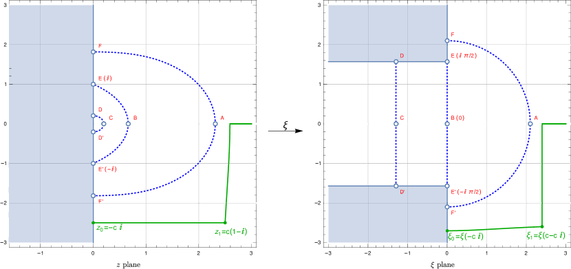
Figure 4: Sketch of the variational path

In Fig. 4 we illustrate both regions; note that Fig. 4 essentially reproduces Figs. 7.1-7.2 from (Olver, 1997, p.376) (except for the variational path). On the left, the $z$ plane and the half-plane $\Re z>0$ is shown; on the right, the $\xi$ plane with the image of $\Re z>0$ is illustrated. In the $\xi$ plane, we depict a few contours and points on them; on the left, the preimages of these contours and points are shown. The shaded regions are the “shadow regions” in Olver’s terminology.

The quantity $\mathcal{V}_{+\infty,z}$ appearing in (A.30) is defined as the total variation of (Olver, 1997, Eq. (7.11), p.376) the function

$$U_{1}(p)=\frac{3p-5p^{3}}{24},\quad p:=(1+z^{2})^{-1/2},$$ (A.31)

along any $\xi$-progressive path connecting $+\infty$ with $z:\Re z>0$. A path $\gamma$ is said to be $\xi$-progressive (Olver, 1997, p.222) if 1) $\gamma$ is a piecewise $C^{2}$-path and 2) $\Re\xi(\gamma)$ is non-increasing as $\gamma$ passes from $+\infty$ to $z$.

The case $\Re z>0$ is not sufficient for us, however, since (A.28) effectively rotates the argument of $H^{(1)}_{\nu}$ in the complex plane by $-\pi/2$. In order to prove (A.5) also for real $w$, we need the expansion of $K_{\nu}(\nu z)$ also when $\arg z=-\pi/2$. Fortunately, the estimates (A.29)-(A.30) remain valid (Olver, 1997, Chapter 10, §8.2) also for $\arg z=-\pi/2$, provided that $\left|z\right|$ is bounded away from 1 and the variational path for $\mathcal{V}_{+\infty,z}$ is correctly constructed (i.e., the path is $\xi$-progressive).

Typically the variational path for $\mathcal{V}_{+\infty,z}$ is chosen so that in the $\xi$ plane the image of the path travels from $\xi(z)$ parallel to the imaginary axis until the real axis is reached, then proceeding along the real axis to $+\infty$, see, e.g., (Olver, 1997, Chapter 10, §7.5), (Setti, 1998, p. 764) or (Bao and Wu, 2006, p. 2133).

However, when $z$ might be of the form $z=-c\mathrm{i}$ for some $c>1$ (as in our setting), this approach is not suitable, since the path must avoid the point $z=-\mathrm{i}$. Instead, for $z=-c\mathrm{i}$ we form a path as follows: travel parallel to the real axis until $z_{1}=c(1-\mathrm{i})$ is reached (satisfying $\arg z_{1}=-\pi/4$), then proceed from $z_{1}$ as described previously. The path is sketched in Fig. 4 (on the left), with its image on the right.

In Section A.6.2 we show that the described path is indeed $\xi$-progressive and estimate the total variation along this path.

A.6.2 Explicit error bounds for the modified Bessel function

Fix any $c>1$ and define $\gamma_{0}(s)=c(s-\mathrm{i})$, $s\in[0,1]$ and $z_{0}=\gamma_{0}(0)=-c\mathrm{i}$, $z_{1}=\gamma_{0}(1)=c(1-\mathrm{i})$. We shall show that

1. $\Re\xi(\gamma_{0}(s))$ is non-decreasing (i.e., the described path from $+\infty$ to $z$ is valid);

2. $\mathcal{V}_{z_{1},z_{0}}\leq\frac{c^{2}(c^{2}+2)}{\sqrt{8}(c^{2}-1)^{2.5}}$, where $\mathcal{V}_{z_{1},z_{0}}$ is the variation of $U_{1}$ along $\gamma_{0}$.

Since the described path connects $z_{0}$ to $z_{1}$ and $z_{1}$ to $+\infty$ with $\Re\xi(z)$ is non-decreasing (and the path is clearly piecewise $C^{2}$), we conclude that the construction ensures a $\xi$-progressive path. Furthermore, the variation $\mathcal{V}_{+\infty,z_{1}}$ can (Bao and Wu, 2006, Eq. (5.13)) be bounded as $\frac{1}{12}+\frac{1}{6\sqrt{5}}+\left(\frac{4}{27}\right)^{1/4}$. Therefore, since $\mathcal{V}_{+\infty,z_{0}}=\mathcal{V}_{+\infty,z_{1}}+\mathcal{V}_{z_{1},z_{0}}$, we can estimate $\mathcal{V}_{+\infty,z_{0}}$ as

$$\mathcal{V}_{+\infty,z_{0}}\leq\frac{1}{12}+\frac{1}{6\sqrt{5}}+\left(\frac{4}{27}\right)^{1/4}+\frac{c^{2}(c^{2}+2)}{\sqrt{8}(c^{2}-1)^{2.5}},\qquad c:=-\Im z_{0}>1.$$ (A.32)

Finally, the estimate (A.32) remains valid when $z_{0}=-c\mathrm{i}$ is replaced by $z=x-c\mathrm{i}$ with any $x>0$:

• If $x\in(0,c]$, then $z$ lies on the described path from $z_{0}$ to $+\infty$, therefore $\mathcal{V}_{+\infty,z}$ is upper-bounded by $\mathcal{V}_{+\infty,z_{0}}$;

• if $x>c$, then $\arg z\in(-\pi/4,0)$ and the bound (Bao and Wu, 2006, Eq. (5.13)) applies; then, $\mathcal{V}_{+\infty,z}$ is upper-bounded by $\frac{1}{12}+\frac{1}{6\sqrt{5}}+\left(\frac{4}{27}\right)^{1/4}$.

The path is $\xi$-progressive.

Since $\xi$ is symmetric around the real axis, i.e., $\xi(\bar{z})=\overline{\xi(z)}$, we have $2\Re\xi(z)=\xi(z)+\xi(\bar{z})$. Define $h(s)=\xi(c(s-\mathrm{i}))+\xi(c(s+\mathrm{i}))$, then $2\Re\xi(\gamma_{0}(s))=h(s)$ and we need to show that $h:[0,1]\to\mathbb{R}$ is non-decreasing.

Let $s\in[0,1]$; denote $z=\gamma(s)=c(s-\mathrm{i})$ and $\omega=\sqrt{1+z^{2}}$. Since $\frac{\,\mathrm{d}\xi}{\,\mathrm{d}z}=\frac{\sqrt{1+z^{2}}}{z}$, we find that

$$h^{\prime}(s) =c\frac{\,\mathrm{d}\xi}{\,\mathrm{d}z}\left(c(s-\mathrm{i})\right)+c\frac{\,\mathrm{d}\xi}{\,\mathrm{d}z}\left(c(s+\mathrm{i})\right)=c\frac{\omega}{z}+c\frac{\bar{\omega}}{\bar{z}}=\frac{\omega\bar{z}+z\bar{\omega}}{c(s^{2}+1)}=\frac{2\Re(\omega\bar{z})}{c(s^{2}+1)}.$$

Since $z=c(s-\mathrm{i})$ satisfies $\arg(z)\in[-\pi/2,-\pi/4]$, it follows that $\arg(z^{2})\in[-\pi,-\pi/2]$ and $\arg(z^{2}+1)\in[-\pi,0)$. Consequently, $\arg(\omega)\in[-\pi/2,0)$. Since $\arg(\bar{z})\in[\pi/4,\pi/2]$, we obtain $\arg(\omega\bar{z})=\arg(\omega)+\arg(z)\in[-\pi/4,\pi/2)$, thus $\Re(\omega\bar{z})>0$. We see that $h^{\prime}(s)$ is positive for $s\in[0,1]$, and $h(s)=2\Re\xi(\gamma_{0}(s))$ is non-decreasing as required.

Estimate of the variation $\mathcal{V}_{z_{1},z_{0}}$.

It is worth recalling that, for a holomorphic function $f$ in a complex domain $D$ containing a piecewise continuously differentiable path $\gamma(s)$, $s\in[s_{0},s_{1}]$, the total variation of $f$ along the path $\gamma$ is defined as

$$\mathcal{V}_{\gamma}(f)=\int_{s_{0}}^{s_{1}}\left|f^{\prime}(\gamma(s))\gamma^{\prime}(s)\right|\,\mathrm{d}s.$$

We have

$$\mathcal{V}_{z_{1},z_{0}}=\int_{0}^{1}\left|\frac{\,\mathrm{d}U_{1}}{\,\mathrm{d}z}\left(p(z)\right)\right|_{z=\gamma_{0}(s)}\left|\gamma_{0}^{\prime}(s)\right|\,\mathrm{d}s.$$

Since

$$\frac{\,\mathrm{d}U_{1}(p)}{\,\mathrm{d}p}=\frac{1-5p^{2}}{8},\quad\frac{\,\mathrm{d}p(z)}{\,\mathrm{d}z}=\frac{-z}{(z^{2}+1)^{3/2}}\quad\text{and}\quad\gamma_{0}^{\prime}(s)=c,$$

the integrand equals

$$\frac{1}{8}\,\left|1-5(1+z^{2})^{-1}\right|\cdot\frac{\left|z\right|}{\left|z^{2}+1\right|^{-3/2}}\cdot c=\frac{c}{8}\cdot\frac{\left|z(z^{2}-4)\right|}{\left|z^{2}+1\right|^{5/2}},\quad z:=c(s-\mathrm{i}).$$

From $\left|z\pm\mathrm{i}\right|=\left|cs-(c\mp 1)\mathrm{i}\right|\geq c\mp 1$ we have $\left|z^{2}+1\right|^{5/2}\geq(c^{2}-1)^{2.5}$. On the other hand, $\left|z\right|\leq c\left|1-\mathrm{i}\right|=c\sqrt{2}$ and $\left|z^{2}-4\right|\leq\left|z\right|^{2}+4\leq 2c^{2}+4$. Since the obtained bound is independent of $z$, the integral satisfies

$$\mathcal{V}_{z_{1},z_{0}}\leq\frac{\sqrt{2}\,c^{2}(2c^{2}+4)}{8(c^{2}-1)^{2.5}}=\frac{c^{2}(c^{2}+2)}{\sqrt{8}(c^{2}-1)^{2.5}},$$

as claimed.

A.6.3 Explicit error bounds for the Hankel function

Let $w\in\mathbb{C}$ be such that $\arg w\in[0;\pi/2)$, then $z=-\mathrm{i}w$ satisfies $\arg z\in[-\pi/2;0)$ and (A.28) with (A.29) imply

$$H^{(1)}_{\nu}(\nu w)=\frac{2}{\pi}\mathrm{e}^{-(\nu+1)\pi\mathrm{i}/2}K_{\nu}(\nu z)=-\mathrm{i}\sqrt{\frac{2}{\pi\nu}}\frac{\mathrm{e}^{-\nu(\xi(-\mathrm{i}w)+\mathrm{i}\pi/2)}}{(1-w^{2})^{0.25}}\left(1+\eta(\nu,-\mathrm{i}w)\right).$$ (A.33)

To see that we can rewrite (A.33) as (A.5), simplify $\xi(-\mathrm{i}w)$ as

$$\xi(-\mathrm{i}w) =(1-w^{2})^{1/2}+\ln\frac{-\mathrm{i}w}{1+\sqrt{1-w^{2}}}=(1-w^{2})^{1/2}-\ln\frac{\mathrm{i}(1+\sqrt{1-w^{2}})}{w}$$

$$=(1-w^{2})^{1/2}-\ln\left(w^{-1}-\mathrm{i}\sqrt{1-w^{-2}}\right)-\pi\mathrm{i}/2$$

$$=(1-w^{2})^{1/2}+\mathrm{i}\arccos(1/w)-\pi\mathrm{i}/2$$

$$=-\mathrm{i}(w^{2}-1)^{1/2}+\mathrm{i}\arccos(1/w)-\pi\mathrm{i}/2.$$

To verify the last equality, notice that $\arg(w^{2}-1)\in[0;\pi)$, thus $\arg(\mathrm{i}(w^{2}-1)^{1/2})\in[\pi/2;\pi)$ and $\arg(\sqrt{1-w^{2}})\in[-\pi/2,0)$, hence $\sqrt{1-w^{2}}=-\mathrm{i}\sqrt{w^{2}-1}$.

Finally, to show (A.6), notice that the function $\frac{1}{12}+\frac{1}{6\sqrt{5}}+\left(\frac{4}{27}\right)^{1/4}+\frac{c^{2}(c^{2}+2)}{\sqrt{8}(c^{2}-1)^{2.5}}$ is decreasing in $c$ for $c>1$ (seen by differentiating with respect to $c$). Since it takes value $2.272365\ldots$ at $c=\pi/2$, for $\nu>1$ and $c=\Re(w)\geq\pi/2$ we have

$$\left|1+\eta(\nu,-\mathrm{i}w)\right|\leq 1+\exp\left(\frac{2\mathcal{V}_{+\infty,-\mathrm{i}w}}{\nu}\right)\,\frac{2\mathcal{V}_{+\infty,-\mathrm{i}w}}{\nu}\leq 1+2\cdot 2.273\mathrm{e}^{2\cdot 2.273}<430.$$

∎

Remark.

The argument above about rewriting $\xi(-\mathrm{i}w)$, in effect, expresses $\xi(z)-z$ as $\mathrm{i}(g(\mathrm{i}z)-\pi/2)$ for $z:\arg z\in[-\pi/2,0)$, with $g$ defined as in Lemma 8. Thus, taking into account the symmetry of $\xi$ around the real axis, Lemma 8 upper bounds the real part of $z-\xi(z)$ for $z:\Re z>0,\,\left|\Im z\right|\geq 1$.

References

- Childs et al. (2003) A. M. Childs, R. Cleve, E. Deotto, E. Farhi, S. Gutmann, and D. A. Spielman, in Proceedings of the 35th Annual ACM Symposium on Theory of Computing, June 9-11, 2003, San Diego, CA, USA, edited by L. L. Larmore and M. X. Goemans (ACM, 2003) pp. 59–68.
- Ambainis (2007) A. Ambainis, SIAM J. Comput. 37, 210 (2007).
- Szegedy (2004) M. Szegedy, in 45th Symposium on Foundations of Computer Science (FOCS 2004), 17-19 October 2004, Rome, Italy, Proceedings (IEEE Computer Society, 2004) pp. 32–41.
- Apers and Sarlette (2019) S. Apers and A. Sarlette, Quantum Inf. Comput. 19, 181 (2019).
- Ambainis et al. (2020) A. Ambainis, A. Gilyén, S. Jeffery, and M. Kokainis, in Proccedings of the 52nd Annual ACM SIGACT Symposium on Theory of Computing, STOC 2020, Chicago, IL, USA, June 22-26, 2020, edited by K. Makarychev, Y. Makarychev, M. Tulsiani, G. Kamath, and J. Chuzhoy (ACM, 2020) pp. 412–424.
- Apers et al. (2021) S. Apers, A. Gilyén, and S. Jeffery, in 38th International Symposium on Theoretical Aspects of Computer Science, STACS 2021, March 16-19, 2021, Saarbrücken, Germany (Virtual Conference), LIPIcs, Vol. 187, edited by M. Bläser and B. Monmege (Schloss Dagstuhl - Leibniz-Zentrum für Informatik, 2021) pp. 6:1–6:13.
- Mohseni et al. (2008) M. Mohseni, P. Rebentrost, S. Lloyd, and A. Aspuru-Guzik, The Journal of Chemical Physics 129, 11B603 (2008).
- Nagaj et al. (2009) D. Nagaj, P. Wocjan, and Y. Zhang, Quantum Information & Computation 9, 1053 (2009).
- Levin and Peres (2017) D. A. Levin and Y. Peres, Markov chains and mixing times, Vol. 107 (American Mathematical Soc., 2017).
- Randall (2006) D. Randall, Computing in Science & Engineering 8, 30 (2006).
- Dyer et al. (1991) M. Dyer, A. Frieze, and R. Kannan, Journal of the ACM (JACM) 38, 1 (1991).
- Lovász and Vempala (2006) L. Lovász and S. Vempala, Journal of Computer and System Sciences 72, 392 (2006).
- Moore and Russell (2002) C. Moore and A. Russell, in International Workshop on Randomization and Approximation Techniques in Computer Science (Springer, 2002) pp. 164–178.
- Aharonov et al. (2001) D. Aharonov, A. Ambainis, J. Kempe, and U. Vazirani, in Proceedings of the thirty-third annual ACM symposium on Theory of computing (2001) pp. 50–59.
- Alagic and Russell (2005) G. Alagic and A. Russell, Physical Review A 72, 062304 (2005).
- Krovi and Brun (2006) H. Krovi and T. A. Brun, Physical Review A 73, 032341 (2006).
- Marquezino et al. (2008) F. L. Marquezino, R. Portugal, G. Abal, and R. Donangelo, Physical Review A 77, 042312 (2008).
- Potoček et al. (2009) V. Potoček, A. Gábris, T. Kiss, and I. Jex, Physical Review A 79, 012325 (2009).
- Shenvi et al. (2003) N. Shenvi, J. Kempe, and K. B. Whaley, Physical Review A 67, 052307 (2003).
- Aaronson and Ambainis (2018) S. Aaronson and A. Ambainis, SIAM J. Comput. 47, 982 (2018).
- Brandão and Horodecki (2013) F. G. S. L. Brandão and M. Horodecki, Quantum Information & Computation 13, 901 (2013).
- Watson (1922) G. N. Watson, A treatise on the theory of Bessel functions (Cambridge University Press, 1922) pp. xviii + 804.
- (23) DLMF, “NIST Digital Library of Mathematical Functions,” http://dlmf.nist.gov/, Release 1.1.4 of 2022-01-15, f. W. J. Olver, A. B. Olde Daalhuis, D. W. Lozier, B. I. Schneider, R. F. Boisvert, C. W. Clark, B. R. Miller, B. V. Saunders, H. S. Cohl, and M. A. McClain, eds.
- Robbins (1955) H. Robbins, The American Mathematical Monthly 62, 26 (1955).
- Mitzenmacher and Upfal (2005) M. Mitzenmacher and E. Upfal, Probability and Computing: Randomized Algorithms and Probabilistic Analysis (Cambridge University Press, 2005).
- Ambainis et al. (2016) A. Ambainis, K. Prūsis, J. Vihrovs, and T. G. Wong, Physical Review A 94, 062324 (2016).
- Paris (1984) R. B. Paris, SIAM Journal on Mathematical Analysis 15, 203 (1984).
- Olver (1997) F. W. J. Olver, Asymptotics and special functions. (A K Peters/CRC Press, 1997) pp. xviii + 572.
- Setti (1998) A. G. Setti, Transactions of the American Mathematical Society 350, 743 (1998).
- Bao and Wu (2006) G. Bao and H. Wu, SIAM Journal on Numerical Analysis 43, 2121 (2006).