Parallel black-box optimization of expensive
high-dimensional multimodal functions via magnitude

Abstract

Building on the recently developed theory of magnitude, we introduce the optimization algorithm EXPLO2 and carefully benchmark it. EXPLO2 advances the state of the art for optimizing high-dimensional ($D\gtrapprox 40$) multimodal functions that are expensive to compute and for which derivatives are not available, such as arise in hyperparameter optimization or via simulations.

1 Introduction

It is a truism that machine learning problems are optimization problems (Sun et al., 2019). Some of the most challenging problems in machine learning involve optimizing multimodal functions without information about derivatives on high-dimensional domains, with hyperparameter optimization (Loshchilov & Hutter, 2016; Koch et al., 2018) an example par excellence. More generally, functions whose values are obtained from complex simulations or experiments are frequently multimodal, and optimizing them is a foundational engineering problem.

Most current optimization algorithms for this regime are not suited for parallel optimization, or have runtime that scales quadratically with dimension; we outline an approach that overcomes both problems simultaneously while outperforming large-scale algorithms (i.e., algorithms that use only sparse linear algebra on any matrices that scale with problem dimension) that do the same. Our EXPLO2 algorithm is a wrapper around an arbitrary large-scale optimizer and serves not least as an initial demonstration of ideas involving the recently developed notion of magnitude (Leinster & Meckes, 2017; Leinster, 2021) that are likely to be more applicable to a wide range of problems in optimization, sampling, machine learning, and other areas.

The paper is structured as follows: §2 introduces the basic concepts of weightings and magnitude that underlie EXPLO2; §3 gives intuition; and §4 gives background on black-box optimization and related work. We describe EXPLO2 in §5 and benchmark it in §6 before making closing remarks in §7. Appendices are after the references.

2 Weightings and magnitude

For background on this section, see §6 of (Leinster, 2021).

A square nonnegative matrix $Z$ is a similarity matrix iff its diagonal is strictly positive. For example, let $t\in(0,\infty)$ and let $d$ be a square matrix whose entries are in $[0,\infty]$ and satisfy the triangle inequality. Then $Z=\exp[-td]$ (where the $[\cdot]$ notation indicates a function applied to the individual entries of a matrix) is a similarity matrix. In this paper, all similarity matrices will be of this form, and $d$ will always be a distance matrix for a finite subset of Euclidean space.

We say that a column vector $w$ is a weighting iff $Zw=1$, where $1$ denotes a vector of all ones. The transpose of a weighting for $Z^{T}$ is called a coweighting. If $Z$ has both a well-defined weighting $w$ and a well-defined coweighting $v$, then its magnitude is $\text{Mag}(Z):=\sum_{j}w_{j}=\sum_{k}v_{k}$.

In the event that $Z=\exp[-td]$ and $d$ is the distance matrix of a finite subset of $\mathbb{R}^{D}$, $Z$ is positive definite (Steinwart & Christmann, 2008), hence invertible, and so its weighting and magnitude are well-defined and unique. More generally, $\text{Mag}(Z)=\sum_{jk}(Z^{-1})_{jk}$ if $Z$ is invertible. The magnitude function $\text{Mag}(t;d)$ is the map $t\mapsto\text{Mag}(\exp[-td])$.

Magnitude is a very general scale-dependent notion of effective size (for finite sets, the effective number of points) that encompasses both cardinality and Euler characteristic, as well as encoding other rich geometrical data (Leinster & Meckes, 2017). Meanwhile, the components of a weighting meaningfully encode a notion of effective size per point (that can be negative “just behind boundaries”) at a given scale (Willerton, 2009; Meckes, 2015; Bunch et al., 2020).

Example 1.

Let $\{x_{j}\}_{j=1}^{3}\subset\mathbb{R}^{2}$ have pairwise distances $d_{jk}:=d(x_{j},x_{k})$ given by $d_{12}=d_{13}=1=d_{21}=d_{31}$ and $d_{23}=\delta=d_{32}$ with $\delta<2$. It turns out that

$$w_{1}=\frac{e^{(\delta+2)t}-2e^{(\delta+1)t}+e^{2t}}{e^{(\delta+2)t}-2e^{\delta t}+e^{2t}};$$

$$w_{2}=w_{3}=\frac{e^{(\delta+2)t}-e^{(\delta+1)t}}{e^{(\delta+2)t}-2e^{\delta t}+e^{2t}}.$$

This is shown in Figure 1 for $\delta=10^{-3}$. At $t=10^{-2}$, the effective sizes of $x_{2}$ and $x_{3}$ are $\approx 0.25$; that of $x_{1}$ is $\approx 0.5$, so the effective number of points is $\approx 1$. At $t=10$, these effective sizes are respectively $\approx 0.5$ and $\approx 1$, so the effective number of points is $\approx 2$. Finally, at $t=10^{4}$, the effective sizes are all $\approx 1$, so the effective number of points is $\approx 3$.

Figure 1: Weighting components for an “isoceles” metric space.

3 Intuition

For large enough values of the scale parameter $t$, the weighting of a finite metric space is proportional to the distribution on the space that maximizes an axiomatically supported notion of diversity (Leinster & Meckes, 2016; Leinster, 2021). Along with this special case, the more general intuition that components of a weighting measure an effective size per point suggests maximizing the differential magnitude due to a new point (which we compute in §C) as a mechanism for efficiently exploring an ambient space.

This idea for “exploration” dovetails with another idea underlying “exploitation.” In $\mathbb{R}^{D}$, $Z=\exp[-td]$ is a radial basis function (RBF) interpolation matrix (Buhmann, 2003) and the equation $Zw=1$ amounts to defining a weighting $w$ as the vector whose components are coefficients for interpolating the unit function. That is, if $\{x_{j}\}_{j=1}^{n}$ are points in $\mathbb{R}^{D}$ with distance matrix $d$ and we have a weighting $w$ satisfying $\sum_{k}w_{k}\exp(-td_{jk})=1$, then in fact $u(x):=\sum_{k}w_{k}\exp(-t|x-x_{k}|)\approx 1$, where $\approx$ indicates an optimal interpolation in the sense of a representer theorem (Schölkopf et al., 2001). In particular, the triangle inequality implies that $u(x_{j}+\delta x_{j})\geq\exp(-t|\delta x_{j}|)$. If now also $f:\mathbb{R}^{D}\rightarrow\mathbb{R}$ and $y_{j}:=f(x_{j})$, then its RBF interpolation is

$$f(x)\approx yZ^{-1}\zeta(x)$$ (1)

where $\zeta_{k}(x):=\exp(-t|x-x_{k}|)$ and we treat $y$ and $\zeta$ respectively as row and column vectors.

We seek to optimize a function by selecting new evaluation points in a way that progressively shifts from exploration (embodied by the differential magnitude due to a new point, for which see Proposition 5.1) to exploitation (embodied by (1), which we obtain at marginal cost). This shift is controlled by an interpretable regularization parameter, and the interpolations are designed to incorporate recent knowledge while requiring constant runtime, even as more points are successively evaluated. For details, see Algorithm 1.

4 Background on black-box optimization

Unconstrained global optimization algorithms can be usefully categorized according to characteristics of the intended objective function. For example, (semi-) differentiable functions are readily optimized using gradient descent or quasi-Newton methods such as L-BFGS (Liu & Nocedal, 1989), whereas if we dispense with any regularity assumptions, a random search is as good an approach as any other.

One intermediate regime of interest is where the objective function is structured and reasonably well behaved (e.g., continuous almost everywhere; Lipschitz continuous, etc.) but only accessible via oracle queries. This regime is referred to in the literature under the terms deriviative-free or black-box optimization (Rios & Sahinidis, 2013; Audet & Hare, 2017). Meanwhile, in an “expensive” regime, the appropriate measure of performance is the current best function value for a given number of function evaluations. For example, the objective function might be defined in terms of a computer simulation that takes a significant amount of time to execute, or an experiment that must be performed.

At a high level of abstraction, global optimization algorithms for expensive black-box functions are about making tradeoffs between exploration of the solution space and exploitation of information that has already been acquired through the course of the algorithm’s execution. A practical and reasonably complete taxonomy of useful techniques is i) metaheuristics such as CMA-ES (Li et al., 2018; Varelas et al., 2018); ii) deterministic algorithms such as DIRECT (Jones & Martins, 2021) or MCS (Huyer & Neumaier, 1999); and iii) surrogate or metamodel-assisted algorithms. In dimension $\lessapprox 5$, metaheuristics and deterministic algorithms are broadly competitive with each other (Sergeyev et al., 2018), but surrogates can yield substantial improvements (Haftka et al., 2016; Vu et al., 2017; Stork et al., 2020; Xia & Shoemaker, 2020).

Surrogate-assisted algorithms can be broadly classified into statistically and geometrically-informed interpolation techniques. The former class of Bayesian optimization (Frazier, 2018) is exemplified by Gaussian process regression (“kriging”); the latter class is exemplified by RBF interpolation.

In Bayesian optimization, a Gaussian process prior is placed on the objective, and after initialization points are selected for evaluation/sampling according to an acquisition function that embodies an explore/exploit tradeoff. While the Bayesian optimization framework is flexible and theoretically appealing, it scales poorly for problems with more than a few tens of dimensions and execution budgets in the thousands. In this regime, statistics are dimensionally cursed, and more geometrically-oriented approaches are needed.

Meanwhile, RBF surrogate techniques for global optimization were introduced in (Gutmann, 2001) and elaborated in (Björkman & Holmström, 2000): here, after initialization, points are selected for evaluation according to the expected “bumpiness” of the resulting surrogate. Subsequent RBF surrogate techniques (Regis & Shoemaker, 2005, 2007) performed exploration by considering distances from previously evaluated points. These RBF surrogate techniques all cycle through a range of distance lower bounds to make exploration/exploitation tradeoffs.

4.1 Related work

Our approach is fairly close to a hybrid of (Regis & Shoemaker, 2005) and (Ulrich & Thiele, 2011). The underlying motivation is that the principled constructs for diversity optimization (“exploration”) and RBF interpolation (to facilitate surrogate “exploitation”) that these approaches respectively build on are actually the same provided only that we use an exponential kernel for the former. Because our notion of diversity optimization is nonlocal, and our unconventional choice of kernel acts as a “gentle funnel,” it is natural to expect that our approach is well-suited to optimizing functions with global structure, as well as multimodal functions, and particularly those functions exhibiting both characteristics.

To keep the runtime per timestep to an acceptably low constant, we borrow an idea of (Booker et al., 1999) to use a “balanced” set of points that includes points with the largest errors for the previous surrogate as well as points with the current most optimal values. For the sake of simplicity, the balancing between these two subsets is determined by the regularizer. Meanwhile, we follow the advice of (Villanueva et al., 2013) for expensive problems by using multiple starting points in conjunction with surrogates.

Work that is only tangentially related but should be mentioned here applies magnitude to primitives in machine learning such as geometry-aware information theory (Posada et al., 2020) and boundary detection (Bunch et al., 2020). These and the present paper indicate that magnitude is fertile ground for growing new ideas in machine learning.

5 Algorithm

The “explore/exploit” (EXPLO2) algorithm described in Algorithm 1 tries to minimize $f:\mathbb{R}^{D}\rightarrow\mathbb{R}$ on $B:=\prod_{j=1}^{D}[\ell_{j},u_{j}]$ with a budget of $N$ function evaluations. EXPLO2 is basically a wrapper around another optimization algorithm (e.g., MATLAB’s default fmincon, which is a large-scale algorithm) that acts on surrogates that gradually shift the balance of a trade between

• exploration, as measured by the differential magnitude of a new point at which to evaluate $f$ relative to the set of points at which $f$ has already been evaluated, and

• exploitation, as measured by an exponential RBF interpolation of $f$ at a mix of points where a previous interpolation had a) the largest errors and b) the most optimal function values.

Both this mix of interpolation points and the tradeoff between exploration and exploitation are controlled by a single regularization term $\lambda:[0,1]\rightarrow\mathbb{R}$, nominally decreasing from $1$ to $0$, e.g. our default choice $\lambda(\tau)=1-\tau$. The course of the algorithm’s execution is shown for the two-dimensional Rastrigin function in Figure 2.

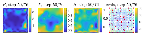
Figure 2: (Top left; center left; center right) Differential magnitude $R$; RBF interpolation $T$; surrogate $S$ after the 25th of 76 function evaluations for the two-dimensional Rastrigin function on $[-5.12,5.12]^{2}$. (Top right) First 25 evaluation points for EXPLO2 overlaid on a contour plot of the objective. (Middle; bottom) As in the top row, but for 50th and 75th of 76 evaluations. Evaluation points ordering is indicated as a transition from red for old points to blue for new points.

The rationale behind an exponential RBF interpolation is simply that this is computed anyway for exploration. That is, the interpolation coefficients are of the form $yZ^{-1}$, where $y$ and $Z=\exp[-td]$ respectively indicate function values and the similarity matrix of evaluation points (see (1) and Algorithm 1). Meanwhile, the limit $t\downarrow 0$ corresponds to an interpolation using very shallow decaying exponentials, which simultaneously avoids degeneracies that arise for $t$ bounded away from zero, mitigates nondifferentiable behavior at interpolation points, and helps make (surrogate) global optima more easily accessible to the internal optimizer.

Algorithm 1 Explore/exploit (EXPLO2) optimizer

0:  Function $f$, lower bounds $\ell$, upper bounds $u$, evaluation budget $N$, optional parameters: number $n_{\parallel}$ of parallel function evaluations (default: $n_{\parallel}=1$), number $n_{\sigma}$ of downsampling points (default: $n_{\sigma}=100$), number $n_{\leftrightarrow}$ of points to estimate exploration range (default: $n_{\leftrightarrow}=100$), number $n_{\downarrow}$ of tries for each surrogate optimization from uniformly random initial points (default: $n_{\downarrow}=3$), explore/exploit regularizer $\lambda$ (default: $\lambda(\tau)=1-\tau$), and initialization strategy (default: uniformly random)

1:  $t\leftarrow\sqrt{\varepsilon}$ // Machine epsilon (see line 13)

2:  Select $N_{0}\leftarrow D+1$ initial points

3:  Evaluate $f$ on the $N_{0}$ initial points

4:  $n\leftarrow N_{0}+1$

5:  while $n<N$ do

6:     if $n>n_{\sigma}$ then

7:        Form $I_{\sigma}$ using $n_{\rho}\approx n_{\sigma}\min(1,\lambda(\frac{n}{N})/\lambda(\frac{1}{N}))$ points with greatest interpolation relative error and $n_{\mu}=n_{\sigma}-n_{\rho}$ points with least function values

8:     else

9:        $I_{\sigma}\leftarrow\{1,2,\dots,n-1\}$

10:     end if

11:     $x_{\sigma}\leftarrow(x_{i})_{i\in I_{\sigma}}$, $y_{\sigma}\leftarrow(y_{i})_{i\in I_{\sigma}}$ // Downsample

12:     $d\leftarrow$ distance matrix for $x_{\sigma}$

13:     $Z\leftarrow\exp[-td]$; // Use $t\downarrow 0$ limit if convenient

14:     $w\leftarrow Z^{-1}1$

15:     $\zeta_{i^{\prime}}(x)\leftarrow\exp(-td(x_{\sigma,i^{\prime}},x))$ // see (1) and Prop. 5.1

16:     $T(x)\leftarrow y_{\sigma}Z^{-1}\zeta(x)$ // RBF exploiTation: see (1)

17:     for $j$ from 1 to $n_{\parallel}$ do

18:        $R\leftarrow\frac{(1-\zeta^{T}w)^{2}}{1-\zeta^{T}Z^{-1}\zeta}$ // exploRation: see Prop. 5.1

19:        $C\leftarrow\min\{2^{D},n_{\leftrightarrow}\}$ corners of bounding box

20:        $R^{\vee}\leftarrow\max_{x\in C}R(x)$

21:        $S\leftarrow\frac{T}{\max y_{\sigma}-\min y_{\sigma}}-\lambda(\frac{n}{N})\frac{R}{R^{\vee}}$ // Surrogate

22:        for $k$ from 1 to $n_{\downarrow}$ do

23:           Minimize $S$ // Using, e.g., fmincon

24:           Keep result iff best so far in current loop

25:        end for

26:        Adjoin best result from line 23 to $x_{\sigma}$

27:        Update $d$, $Z$, $w$ and $\zeta$ as in lines 12-15

28:     end for

29:     Memorialize/evaluate in parallel the $n_{\parallel}$ new points

30:     Get relative errors of RBF interpolation for downsampling per lines 7, 11, and 16

31:     $n\leftarrow n+n_{\parallel}$

32:  end while

32:  $(x_{i},y_{i})_{i=1}^{N}$

The definition of $R(x)$ in Algorithm 1 arises from

Proposition 5.1.

Let $Z$ be positive definite and consider a positive definite matrix of the form $Z[\zeta]:=\left(\begin{smallmatrix}Z&\zeta\\ \zeta^{T}&1\end{smallmatrix}\right)$. Then

$$\text{Mag}(Z[\zeta])=\text{Mag}(Z)+\frac{(1-\zeta^{T}w)^{2}}{1-\zeta^{T}Z^{-1}\zeta}.\qed$$ (2)

EXPLO2 “just” requires a positive definite metric space in the sense of (Meckes, 2013) and a suitable solver for the surrogate functions. In particular, any subset of Euclidean space is positive definite, as is any ultrametric space or weighted tree. In the Euclidean setting, we can always use an extremum of a continuous RBF interpolation to approximate an extremum of the underlying black-box function: while there are no guarantees on the errors that result, in practice such errors can usually be reasonably expected to be tolerably small. EXPLO2 is thus applicable de novo to a wide range of discrete problems.

It is important to note that the runtime of EXPLO2 is not directly affected by the dimension $D$. The impact of dimension is felt mainly through the inner optimizer, which for large-scale algorithms such as fmincon is typically linear. However, while we use the default value $n_{\sigma}=100$ at all times, it is conceivable that one might want $n_{\sigma}=O(D)$, which would nominally introduce a cubic runtime dependence on $D$ (i.e., even worse than CMA-ES). To avoid this, we note that experiments on time series (described in §D) indicate that it is possible to get good approximations to weightings from nearest neighbors alone, even in problems with hundreds of thousands of dimensions. Along similar lines, an efficient approximate nearest neighbor algorithm (Datar et al., 2004; Andoni et al., 2018; Li et al., 2020) could be used to efficiently create a sparse similarity matrix $Z$, yielding a large-scale algorithm, and probably one with little performance penalty.

6 Benchmarking

6.1 Algorithms for comparison

Most black-box optimization algorithms are tailored to problems in dimension $\lessapprox 20$ and/or inexpensive functions. On one hand, many optimization algorithms suitable for higher-dimensional applications (including variants of the popular CMA-ES and L-BFGS algorithms) require thousands or tens of thousands of function evaluations per dimension to yield acceptable results (Varelas et al., 2018; Varelas, 2019). On the other hand, even state-of-the-art Bayesian optimization algorithms such as SMAC-BBOB (Hutter et al., 2013) or (Eriksson et al., 2019) are generally not competitive on problems with more than a few tens of dimensions. In short, the list of candidate algorithms for optimizing high-dimensional expensive functions is not long, and it becomes shorter when considering multimodal functions.

For low evaluation budgets in dimension $\lessapprox 40$, NEWUOA (Powell, 2006; Ros, 2009), MCS, and GLOBAL (Csendes, 1988; Csendes et al., 2008) are the best algorithms on the BBOB testbed (Hansen et al., 2009, 2010). Meanwhile, (Brockhoff, 2015) points out that for expensive black-box optimization using surrogates in dimension $\lessapprox 40$,

the three algorithms SMAC-BBOB (for very low budgets below $\approx 3\cdot D$ function evaluations), NEWUOA (for medium budgets), and lmm-CMA-ES (for relatively large budgets of $\geq 30\cdot D$ evaluations) build a good portfolio that constructs the upper envelope over all compared algorithms for almost all problem groups.

With this in mind, a representative set of algorithms to benchmark against for low-dimensional, expensive, multimodal functions is NEWUOA, MCS, GLOBAL, SMAC-BBOB, and *-CMA-ES with * $\in$ {lmm, DTS, lq}. Of these, only NEWUOA is well-suited to problems with hundreds of dimensions (indeed, most of these algorithms have not even been benchmarked for dimension $40$ in COCO (Hansen et al., 2021) as of this writing, and

• while NEWUOA scales to hundreds of dimensions, its time complexity ranges between quadratic and quintic in dimension–with quadratic or cubic the case in practice and as benchmarked (Ros, 2009);

• MCS is unsuitable for high-dimensional problems as it relies on partitioning the search space;

• GLOBAL is unsuitable for high-dimensional problems because it relies on clustering (Assent, 2012);

• as a Bayesian optimization technique, SMAC-BBOB is not suited to high-dimensional problems;

• for “noisy and multimodal functions, the speedup [of surrogate-assisted variants of CMA-ES relative to CMA-ES] …vanishes with increasing dimension” (Kern et al., 2006); i.e., “lmm- and DTS-CMA-ES become quickly computationally infeasible with increasing dimension, hence their main application domain is in moderate dimension” (Hansen, 2019), where they embody the state of the art for relatively large budgets of $\geq 30\cdot D$ evaluations (Bajer et al., 2019).

Finally, since EXPLO2 is (as benchmarked) a wrapper around fmincon, it also makes sense to compare the performance of these two algorithms.

6.2 Results

Results from experiments according to (Hansen et al., 2016b, a) on the BBOB benchmark functions given in (Hansen et al., 2009) are presented in Figures 3-10 (see also §G-K). The experiments were performed and plots were produced with COCO (Hansen et al., 2021), version 2.4.

Because of the runtime overhead of EXPLO2, our experiments used a fixed budget of 25 function evaluations per dimension. As (Hansen et al., 2016b) points out, algorithms are only comparable up to the smallest budget given to any of them, corresponding in this case to $\log_{10}25\approx 1.40$ on the horizontal axis for Figures 3 and 7. This corresponds in our case exactly to the location of crosses ($\times$), which indicate where bootstrapping of experimental data begins to estimate results for larger numbers of function evaluations. At the same time, we used $n_{\parallel}=32$, and $\log_{10}(25/32)\approx-0.107$. Thus allowing for parallel resources (see §6.3) suggests comparing EXPLO2 at the value $\log_{10}25$ on the horizontal axes with the other algorithms at $\log_{10}(25/32)$, except for *-CMA-ES, which is parallelizable.

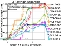
Figure 3: Empirical cumulative distribution of simulated (bootstrapped) runtimes, measured in number of objective function evaluations divided by dimension (FEvals/DIM) in dimension 20 and for those targets in $10^{[-8..2]}$ that have just not been reached by the best algorithm from BBOB 2009 in a given budget of $k$ $\times$ DIM, with $31$ different values of $k$ chosen equidistant in logscale within the interval $\{0.5,\dots,50\}$. Crosses ($\times$) indicate where experimental data ends and bootstrapping begins; algorithms are not comparable after this point. EXPLO2 used default options except for $n_{\parallel}=32$. While *-CMA-ES outperforms EXPLO2 here, in high dimensions only large-scale variants of CMA-ES are appropriate for most purposes, and EXPLO2 outperforms the best of these on structured multimodal functions: see Figures 11-14.

Figure 4: As in Figure 3, but for $f_{7}$ and $f_{15}$.

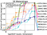
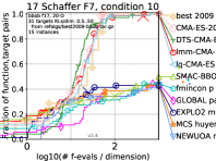
Figure 5: As in Figure 3, but for $f_{16}$ and $f_{17}$.

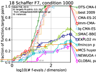
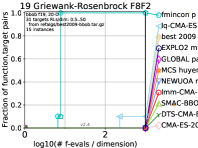
Figure 6: As in Figure 3, but for $f_{18}$ and $f_{19}$. Note that Figures 13 and 14 present an alternative analysis for $f_{19}$ in dimensions 20 and 320, respectively.

Figure 7: As in Figure 3, but for $D=40$. Note that fewer algorithms have benchmark data for $D=40$ than for $D=20$.

Figure 8: As in Figure 3, but for $f_{7}$ and $f_{15}$ and $D=40$.

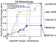
Figure 9: As in Figure 3, but for $f_{16}$ and $f_{17}$ and $D=40$.

Figure 10: As in Figure 3, but for $f_{18}$ and $f_{19}$ and $D=40$.

Our experiments show that EXPLO2 consistently outperforms fmincon on the sorts of problems for which it was designed, viz., multimodal functions with adequate global structure ($\{f_{15},\dots,f_{19}\}$), with the exception of the function $f_{19}$, which has many shallow minima. On the other hand, for most other problems in the BBOB suite (with the notable exceptions of $f_{3}$, $f_{4}$, and $f_{7}$, which respectively gauge the ability to exploit separability, not rely on symmetry, and to avoid getting trapped on plateaux), EXPLO2 does worse than fmincon.

EXPLO2 outperforms NEWUOA on $f_{15}$, $f_{17}$, and $f_{18}$, while the converse is true for $f_{16}$ and $f_{19}$, suggesting that EXPLO2 (as a wrapper around fmincon) is best for multimodal functions with global structure that are not rugged, repetitive, or with many shallow minima. In other words, EXPLO2 is best for problems with fairly structured landscapes. Even without accounting for the benefits of parallelism, EXPLO2 is arguably the best available method besides *-CMA-ES for problems in dimension $\approx 20$ to $40$; once we do account for parallelism and/or in higher dimensions, only certain members of *-CMA-ES perform comparably: see §6.3.

Meanwhile, in high enough dimensions, *-CMA-ES also ceases to be practical, with the exception of large-scale variants. EXPLO2 also tied with or outperformed all of the large-scale algorithms benchmarked in (Varelas, 2019) on the large-scale version of every BBOB function in $\{f_{15},\dots,f_{24}\}$ for dimensions 80, 160, and 320 (Elhara et al., 2019) with a budget of 2 evaluations/dimension. EXPLO2 still performed fairly close to (and sometimes still better than) other algorithms in dimension 640 on the same budget per dimension. Finally, it is reasonable to hypothesize that a relative performance degradation in dimension 640 could be mitigated by replacing the inner fmincon optimization with L-BFGS.

Because these experiments did not facilitate plots that conveyed meaningful information (an “expensive plot” option is not available in COCO for the large-scale BBOB suite), we also performed a more ad hoc comparison of EXPLO2 to VD-CMA-ES (Akimoto et al., 2014), the best performing large-scale algorithm for structured multimodal functions in (Varelas, 2019). As Figures 11-14 show, EXPLO2 performs better, regardless of parallelism.

Figure 11: A comparison of VD-CMA-ES and EXPLO2 on the Rastrigin function (without rotations or shifts, but otherwise corresponding to $f_{15}$ in the BBOB testbed) on $[-5.12,5.12]^{D}$ for $D=20$ and a budget of 500 function evaluations. For VD-CMA-ES, various initial step sizes $\sigma_{init}$ were selected as shown and logging is intermittent; meanwhile, for EXPLO2, we considered $n_{\parallel}\in\{1,32\}$. Each algorithm/parameter pair was run three times, all shown. Note that the initialization phase of VD-CMA-ES is not plotted.

Figure 12: As in Figure 11, but for $D=320$ and a budget of 1600.

Figure 13: As in Figure 11, but for the Griewank-Rosenbrock function F8F2 (without rotations or shifts, but otherwise corresponding to $f_{19}$ in the BBOB testbed) on $[-5,5]^{D}$ for $D=20$. Note that VD-CMA-ES often terminates before the budget is reached.

Finally, in an experiment shown in §K, we found that EXPLO2 outperformed differential evolution and had performance almost indistinguishable from CMA-ES on the mixed-integer version of $f_{15}$ (Tušar et al., 2019) in dimension $D=20$ (the only function/dimension pair we tried among the mixed-integer suite (Tušar et al., 2019)).

To summarize, as the dimension of structured multimodal problems grows, EXPLO2 outperforms NEWUOA, particularly when taking parallelism into account; meanwhile, the quadratic scaling with dimension of non-large-scale *-CMA-ES algorithms puts them at an increasing disadvantage since EXPLO2 has essentially no runtime dependence on dimension other than through its inner solver, which here is the default large-scale interior-point fmincon algorithm. Finally, on structured multimodal functions, EXPLO2 outperforms VD-CMA-ES, which is otherwise the best-performing large-scale algorithm that we are aware of.

6.3 Parallel performance

While EXPLO2 is parallelized (at marginal cost to performance), to the best of our knowledge no competing technique is except for *-CMA-ES. Indeed, as (Gao et al., 2017) points out, most surrogate-based derivative-free optimizers–including NEWUOA–require sequential function evaluations. Though parallel algorithms exist (Haftka et al., 2016; Rehbach et al., 2018; Xia & Shoemaker, 2020), these are relatively few in number outside the context of Bayesian optimization (which is unsuitable for high-dimensional problems), and parallel techniques appropriate for high-dimensional problems have been considered in our design and/or benchmarking.

With this in mind, since our experiments use $n_{\parallel}=32$, exceeding our per-dimension evaluation budget of 25, it is obvious that EXPLO2 can outperform any of the competing algorithms considered here on the number of rounds of parallel function evaluations, except for *-CMA-ES, which becomes (depending on the variant employed) ill-suited for use or less performant than EXPLO2 in high dimensions.

7 Remarks

As mentioned above, it would be interesting–and likely useful–to replace fmincon with, e.g., L-BFGS.

Figure 14: As in Figure 13, but for $D=320$ and a budget of 1600.

Though the runtime overhead of EXPLO2 scales favorably with dimension, it is still high for any given function evaluation: the surrogate is complicated and even a large-scale inner optimizer takes resources. EXPLO2 is therefore only suited for high-dimensional functions that are expensive to evaluate. While as mentioned earlier, hyperparameter optimization or simulation-defined functions are in this vein, it will generally be advisable to evaluate the suitability of *-CMA-ES as well in any particular application.

While EXPLO2 seeks to balance exploration and exploitation through a regularizer, an approach in the vein of (Bischl et al., 2014) (cf. (Xia & Shoemaker, 2020)) is also reasonable and lends itself to parallel execution. The idea here would be to consider the RBF interpolation and the differential magnitude as proxy objectives and evaluate the actual objective function in parallel at points on the Pareto front. This approach is likely to be useful for “illuminating” the search space or providing “quality diversity” (Mouret & Clune, 2015; Pugh et al., 2016; Fontaine et al., 2020; Chatzilygeroudis et al., 2021) in a way that focuses on diversity promotion versus the related idea (Vassiliades et al., 2017) of niching techniques for multimodal optimization.

We have experimented with alternative choices for $t$ in Algorithm 1 besides $\sqrt{\varepsilon}$, but all yielded inferior results (the exact $t=0$ limit caused trouble with fmincon). However, our experiments were not exhaustive or conclusive: it is possible that a more substantial modification of Algorithm 1 that also lets $t$ vary would yield superior results. Nevertheless, we were not able to identify a competitive variant, let alone a clearly superior one.

Finally, while we have already pointed out that differential magnitude is an attractive way to perform exploration for Bayesian optimization, it may also be useful for generating proposals in Markov chain Monte Carlo methods, including fast parallel algorithms such as those in (Huntsman, 2020, 2021). More generally, magnitude-based methods hold promise for many other problems in machine learning.

Appendix A Outline of appendices

This appendices are organized as follows:

• §B discusses the limit $t\downarrow 0$ on (co)weightings;

• §C discusses the differential magnitude of a point;

• §D discusses how to compute (co)weightings in dimension $>10^{5}$ in the context of time series analysis, with an eye towards more general problems of similar scale using similarity search;

• §E discusses the efficient computation of weightings from the perspective of linear algebra;

• §F contains plots generated using IOHAnalyzer;

• §G contains plots generated using COCO for scaling of runtime with dimension;

• §H contains plots generated using COCO for runtime distributions (ECDFs) per function for $D=20$;

• §I contains plots generated using COCO for runtime distributions (ECDFs) per function for $D=40$;

• §J contains plots generated using COCO for the large-scale BBOB suite;

• §K contains a plot generated using COCO for the mixed-integer BBOB suite;

• §L contains MATLAB source code for EXPLO2;

• §M contains MATLAB source code for benchmarking.

Appendix B The scale $t=0$

The limit $t\uparrow\infty$ of (co)weightings and the magnitude function is uninteresting, since the (co)weightings are (co)vectors of all ones, so the limiting value of the magnitude function is just the number of points in the space under consideration. However, the limit $t\downarrow 0$ contains more detailed structural information:

Lemma B.1.

For $d\in GL(n,\mathbb{R})$ the solution to $\exp[-td]w(t)=1$ has the well-defined limit $w(0):=\lim_{t\downarrow 0}w(t)=\frac{d^{-1}1}{1^{T}d^{-1}1}$. Similarly, the solution to $v(t)\exp[-td]=1$ has the limit $v(0)=\frac{1^{T}d^{-1}}{1^{T}d^{-1}1}$.

Proof (sketch).

We have the first-order approximation $(11^{T}-td)w(t)\approx 1$. Applying the Sherman-Morrison-Woodbury formula (Horn & Johnson, 2012) and L’Hôpital’s rule yields the result. ∎

Appendix C The differential magnitude of a point

Define $M:=\left(\begin{smallmatrix}A&B\\ C&D\end{smallmatrix}\right)$. Block inversion yields the formula

$$\begin{pmatrix}A^{-1}+A^{-1}B(M/A)^{-1}CA^{-1}&-A^{-1}B(M/A)^{-1}\\ -(M/A)^{-1}CA^{-1}&(M/A)^{-1}\end{pmatrix}$$

for $M^{-1}$, where the Schur complements are given by $M/D:=A-BD^{-1}C$ and $M/A:=D-CA^{-1}B$, and they satisfy $(M/A)^{-1}=D^{-1}+D^{-1}C(M/D)^{-1}BD^{-1}$ and $(M/D)^{-1}=A^{-1}+A^{-1}B(M/A)^{-1}CA^{-1}$.

If $C=B^{T}$ and $A$, $D$, and $M$ are all positive definite, then Theorem 7.7.7 of (Horn & Johnson, 2012) yields that $M/A$, $M/D$, and $M$ are also all positive definite. With this in mind (and similarly to (Bunch et al., 2020)), let $Z$ be positive definite and consider a positive definite matrix of the form

$$Z[\zeta]:=\begin{pmatrix}Z&\zeta\\ \zeta^{T}&1\end{pmatrix}.$$ (3)

The relevant Schur complement is

$$Z[\zeta]/Z=1-\zeta^{T}Z^{-1}\zeta,$$

so $Z[\zeta]^{-1}$ equals

$$\ \begin{pmatrix}Z^{-1}&0\\ 0&0\end{pmatrix}+\frac{1}{1-\zeta^{T}Z^{-1}\zeta}\begin{pmatrix}Z^{-1}\zeta\zeta^{T}Z^{-1}&-Z^{-1}\zeta\\ \zeta^{T}Z^{-1}&1\end{pmatrix}$$

$$= \ \begin{pmatrix}Z^{-1}&0\\ 0&0\end{pmatrix}+\frac{1}{1-\zeta^{T}Z^{-1}\zeta}\begin{pmatrix}-Z^{-1}\zeta\\ 1\end{pmatrix}\begin{pmatrix}-\zeta^{T}Z^{-1}&1\end{pmatrix}$$

so that if $w=Z^{-1}1$ and $w[\zeta]:=Z[\zeta]^{-1}1$ are respectively the weightings of $Z$ and $Z[\zeta]$, then

$$w[\zeta]=\begin{pmatrix}w\\ 0\end{pmatrix}+\frac{1-\zeta^{T}w}{1-\zeta^{T}Z^{-1}\zeta}\begin{pmatrix}-Z^{-1}\zeta\\ 1\end{pmatrix}.$$ (4)

This yields

Proposition C.1.

$$\text{Mag}(Z[\zeta])=\text{Mag}(Z)+\frac{(1-\zeta^{T}w)^{2}}{1-\zeta^{T}Z^{-1}\zeta}.\qed$$ (5)

It is tempting to try to use this result to try to establish the conjecture of (Yevseyeva et al., 2019) that magnitude is submodular on Euclidean point sets, but there is a simple counterexample:

Example 2.

Let $\Omega=\{(1,0),(0,1),(-1,0),(2,0)\}$ endowed with Euclidean distance; let $X=\{(1,0),(0,1)\}$; let $x_{1}=(-1,0)$, and $x_{2}=(2,0)$. Then (abusing notation) $\text{Mag}(X\cup\{x_{1}\})+\text{Mag}(X\cup\{x_{2}\})\approx 4.1773$ while $\text{Mag}(X\cup\{x_{1},x_{2}\})+\text{Mag}(X)\approx 4.1815$.

Still, for $t\rightarrow\infty$ there is an asymptotic inclusion-exclusion formula for magnitudes of compact convex bodies, as pointed out by (Gimperlein & Goffeng, 2021). In this sense the magnitude is approximately submodular. This suggests using the standard greedy approach for approximate submodular maximization (Nemhauser et al., 1978; Krause & Golovin, 2014) despite the fact that we do not have any theoretical guarantees.

On the other hand, if $Z=\exp[-td]$, $\zeta=\exp[-t\delta]$, and we write $\omega=d^{-1}1$, we have the following:

Lemma C.2.

$$\frac{(1-\zeta^{T}w)^{2}}{1-\zeta^{T}Z^{-1}\zeta}=o(t)+$$

$$t\left(\frac{\delta^{T}\omega-1}{1^{T}\omega-t}\right)^{2}\frac{1^{T}\omega-t}{-1+2\delta^{T}\omega+\delta^{T}[(1^{T}\omega)d^{-1}-\omega\omega^{T}]\delta}.$$ (6)

Proof.

Using $Z\approx 11^{T}-td$, the Sherman-Morrison formula gives $Z^{-1}\approx-\frac{1}{t}\left(d^{-1}+\frac{\omega\omega^{T}}{t-1^{T}\omega}\right)$. A line of algebra yields $w=Z^{-1}1\approx\frac{\omega}{1^{T}\omega-t}$, and similarly $1-\zeta^{T}w\approx t\frac{\delta^{T}\omega-1}{1^{T}\omega-t}$. Now

$$\zeta^{T}Z^{-1}\zeta \approx-\frac{1}{t}(1^{T}-t\delta^{T})\left(d^{-1}+\frac{\omega\omega^{T}}{t-1^{T}\omega}\right)(1-t\delta)$$

$$=\frac{1^{T}\omega}{1^{T}\omega-t}-2t\frac{\delta^{T}\omega}{1^{T}\omega-t}-t\delta^{T}\left(d^{-1}+\frac{\omega\omega^{T}}{t-1^{T}\omega}\right)\delta$$

$$\approx\frac{(1^{T}-2t\delta^{T})\omega-t\delta^{T}[(1^{T}\omega)d^{-1}-\omega\omega^{T}]\delta}{1^{T}\omega-t},$$

so

$$1-\zeta^{T}Z^{-1}\zeta\approx t\frac{-1+2\delta^{T}\omega+\delta^{T}[(1^{T}\omega)d^{-1}-\omega\omega^{T}]\delta}{1^{T}\omega-t},$$

from which the result follows. ∎

Another way to write (C.2) is using the identities

$$(\delta^{T}\omega-1)^{2}=\begin{pmatrix}\delta^{T}&1\end{pmatrix}\begin{pmatrix}\omega\omega^{T}&-\omega\\ -\omega^{T}&1\end{pmatrix}\begin{pmatrix}\delta\\ 1\end{pmatrix}$$

and

$$-1+2\delta^{T}\omega+\delta^{T}[(1^{T}\omega)d^{-1}-\omega\omega^{T}]\delta=$$

$$\begin{pmatrix}\delta^{T}&1\end{pmatrix}\begin{pmatrix}(1^{T}\omega)d^{-1}-\omega\omega^{T}&\omega\\ \omega^{T}&-1\end{pmatrix}\begin{pmatrix}\delta\\ 1\end{pmatrix}.$$

In $\mathbb{R}^{n}$, we have the “far-field” asymptotic $\delta\sim s(\delta)1$, where $s(\cdot)$ is any function on tuples that takes values between the minimum and maximum (e.g., an order statistic or quasi-arithmetic mean). That is, in the limit $t\rightarrow 0$ and $\delta\rightarrow\infty$, (C.2) takes the form (with an obvious but helpful abuse of notation)

$$\frac{(1-\zeta^{T}w)^{2}}{1-\zeta^{T}Z^{-1}\zeta}\sim$$

$$\frac{t}{1^{T}\omega}\cdot\frac{\begin{pmatrix}s1^{T}&1\end{pmatrix}\begin{pmatrix}\omega\omega^{T}&-\omega\\ -\omega^{T}&1\end{pmatrix}\begin{pmatrix}s1\\ 1\end{pmatrix}}{\begin{pmatrix}s1^{T}&1\end{pmatrix}\begin{pmatrix}(1^{T}\omega)d^{-1}-\omega\omega^{T}&\omega\\ \omega^{T}&-1\end{pmatrix}\begin{pmatrix}s1\\ 1\end{pmatrix}}+o(t).$$

Expanding this out, we find that the $s^{2}$ term in the denominator is zero, and we end up with

$$\frac{(1-\zeta^{T}w)^{2}}{1-\zeta^{T}Z^{-1}\zeta}\sim\frac{s(\delta)}{2}t+o(t).$$ (7)

That is, the change in magnitude is asymptotically linear with respect to distance. Among other things, this provides a foundation for building diverse point sets in unbounded regions of Euclidean space by maximizing the ratio of the increase of magnitude and a suitable function $s(\delta)$.

Appendix D Coweightings in dimension $>10^{5}$ and time series analysis

Here we sketch how coweightings can reliably identify “boundary” elements of large datasets in high dimension within the restricted context of time series analysis. Efficient analogues of the construction below can likely be produced in more general settings using similarity search techniques (Zezula et al., 2006), provided they are available.

Consider a reasonably nice time series $\{x_{j}\}_{j=1}^{n+L-1}$ with $x_{j}\in\mathbb{R}$ and $n\gg L\gg 1$. By considering contiguous subsequences of length $L$, we obtain $n$ points $x^{[L]}_{j}:=(x_{j},\dots,x_{j+L-1})\in\mathbb{R}^{L}$. The matrix profile (Yeh et al., 2016) operates on this latter representation to find maximally conserved motifs, anomalous subsequences, etc. In particular, the matrix profile efficiently yields (an anytime approximation of) a sequence of pairs $(d_{j},\mathcal{I}(j))$ such that $x^{[L]}_{\mathcal{I}(j)}$ is the nearest neighbor to $x^{[L]}_{j}$ under $d^{(z)}$, with $d^{(z)}(x^{[L]}_{j},x^{[L]}_{\mathcal{I}(j)})=d_{j}$, and where $d^{(z)}$ is a variant of the $\ell^{2}$ distance obtained by subtracting mean values and normalizing by the standard deviations of arguments. It turns out that the information provided by the matrix profile can efficiently address many if not most problems in basic time series analysis.

In fact, the index alone $\mathcal{I}$ suffices to yield impressive information about time series when coupled with a coweighting. The idea is as follows: let $d$ be a matrix of size $n$ with all entries equal to $\infty$ except for a zero diagonal and $d_{j,\mathcal{I}(j)}:=d_{j}$ (or any other finite number on the right hand side). Then the matrix $Z(0):=\lim_{t\downarrow 0}\exp(-td)$ is a 0-1 matrix with precisely two nonzero entries per row. While this matrix is obviously singular, dividing a row vector of all ones on the left by it generally yields a reasonably nice result: i.e., the number of singular entries is reasonably small if not zero. Setting these to zero (or exploiting the structure of the problem to justify interpolation), the resulting approximate coweighting yields information about motifs which are presumably extremal in some sense.

Figures 15-18 show plots of subsequences with successive highest and lowest coweightings for (slightly smoothed) coordinate data in a localization application (Kaluža et al., 2010) with $n=163861$ and $L=1000$. The figures suggest that these subsequences are near each other and respectively on or “adjacent to” a “boundary” of $\{x^{[L]}_{j}\}_{j=1}^{n}\subset\mathbb{R}^{L}$, since their coweightings are large in absolute value and approximately cancel. Note that in some cases the pairing is not exact, but the coweighting values indicate this and can suggest alternative pairings.

Figure 15: Plots (for the first spatial coordinate of data from (Kaluža et al., 2010)) of $x^{[L]}_{j}$ after subtracting means and normalizing by standard deviations. From right to left, we show pairs of successively largest negative and positive values of the (approximate) coweighting $\hat{v}$ in blue and red, respectively. The legend entries are of the form $(j,\hat{v}_{j})$.

Figure 16: As in Figure 15, but for the second spatial coordinate of data from (Kaluža et al., 2010). Note that the pairing is not exact, but the coweighting values indicate this.

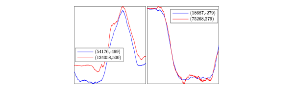
Figure 17: An improved pairing for some of the data in Figure 16. Not shown: $x^{[L]}_{20195}$ in the center left panel of Figure 16 and the data in the leftmost panel of Figure 16 also match decently.

Figure 18: As in Figure 15, but for the third spatial coordinate of data from (Kaluža et al., 2010). Note that the pairing is not exact, but the coweighting values indicate this. It seems likely that in this particular case these points “interfere” with each other since there are obvious structures that are roughly conserved across the plots shown.

To reinforce the geometrical characterization above, we applied the UMAP dimension reduction algorithm (McInnes et al., 2018) to subsets of $\{x^{[L]}_{j}\}_{j=1}^{n}$ for the first spatial coordinate of data from (Kaluža et al., 2010) (the other spatial coordinates yield qualitatively similar results that we do omit for economy). Figure 19 shows how this approach captures salient aspects of the geometry. Figure 20 takes a more structured approach by considering the union of $x^{[L]}_{j}$ with i) large (in absolute value) coweightings; ii) equispaced indices; and iii) a sample stratified by coweighting values (i.e., the lowest decile of coweights corresponds to 10% of the [sub]sample, and so on). Figure 20 also highlights the nine points resulting from an erosion-type procedure as shown in Figure 21. Specifically, we consider the points whose coweighting is above a threshold $\tau$, and exploit the problem structure to isolate points with the largest coweighting within an index range of $\pm L/2$. We then compute the dissimilarity at $t=0$, and check to see if any of its coweighting components are negative. We then take the largest $\tau$ that produces a nonnegative coweighting on these isolated points: in this case $\tau\approx 119.8$. This procedure evidently retains reliable “witnesses” to the geometry.

Figure 19: (L) UMAP applied to $\{x^{[L]}_{j}\}_{j=1}^{n}$ after normalization. Points are colored by (approximate) coweighting components, and sized by the absolute value of these components. While this accurately captures the intrinsic 1-dimensional geometry of the data, this is actually uninformative from the point of view of bulk geometry. (R) UMAP applied to $\{x^{[L]}_{j}\}_{j\equiv 1\text{ mod }10}$ after normalization. Here the colocation of positively and negatively coweighted points is visually apparent, as is their distribution along “ridges” in the data.

Figure 20: UMAP applied to $\{x^{[L]}_{j}\}_{j\in J_{\tau}\cup J_{=}\cup J_{v}}$ after normalization. Here $J_{\tau}$ is the set of indices with (approximate) coweights above $\tau\approx 119.8$, $J_{=}$ is a set of $\approx 5000$ equispaced indices, and $J_{v}$ is a set of $\approx 5000$ indices corresponding to an approximately uniformly stratified random sample according to the coweighting. Here the “boundaryness” of points with large (approximate; in absolute value) coweighting is apparent. Black circles indicate the nine points depicted in the right panel of Figure 21.

Figure 21: (L) Plots of normalized $x^{[L]}_{j}$ for $j$ such that $|\hat{v}_{j}|>\tau$. (R) Plots of the nine $x^{[L]}_{j}$ resulting from an “erosion-like” procedure that repeatedly discards points with negative (co)weighting components. These remaining points evidently capture the bulk behavior of the larger set in the left-hand panel.

Appendix E Efficiently computing weightings

Besides a clever use of inclusion/exclusion to accelerate weighting computations in the cases where a few points are added and/or perturbed (for which see §C and §2 of (Bunch et al., 2020)), we briefly discuss methods for efficiently solving the weighting equation $Zw=1$.

For the usual metric on $\mathbb{R}^{D}$, the similarity matrix $Z$ is positive definite, so we get a reproducing kernel Hilbert space to which Mercer’s theorem applies. In practice this amounts to the existence of a Cholesky decomposition $Z=LL^{T}$ and a positive square root.

However, the ideal method to solve $Zw=1$ at scale is to use efficient solvers that exploit kernel structure in a more detailed way. As (Rebrova et al., 2018) points out, “kernel matrices are good candidates for hierarchical low-rank solvers” like (Rouet et al., 2016; Chenhan et al., 2017) that offer subquadratic performance.

Still, using a special-purpose solver may not be worthwhile at intermediate scales. As an alternative, the system $Zw=1$ can be solved without explicitly forming the entire matrix $Z$ via the the (preconditioned) conjugate gradient method, which has computational complexity $O(\text{nnz}\cdot\sqrt{\kappa})$, where nnz and $\kappa$ respectively denote the number of nonzero entries and the condition number of the matrix (Shewchuk, 1994). Moreover, we can improve on this complexity with a good initial guess for a weighting: this is likely to be of particular relevance for iterative algorithms.

The conjugate gradient approach is not really worthwhile unless we can set small entries of $Z$ to zero (so that $\text{nnz}\ll n^{2}$) while maintaining positive definiteness. Although “hard thresholding” generic positive definite matrices in this way generally does not preserve the property of positive definiteness (Guillot & Rajaratnam, 2012), it does for sufficiently large $t$ (e.g., above the minimal value that ensures a weighting is positive; cf. Example 6.3.27 of (Leinster, 2021)), and probably more generally.

In any event, we can hard-threshold $Z$ and efficiently solve the resulting system, exploiting positive definiteness if we have it by applying the conjugate gradient method. One way to produce such a sparse version of $Z$ de novo without forming the full matrix is to follow the approach of §D and only compute entries for nearby points. Ultimately, hard thresholding requires an efficient similiarity search (Zezula et al., 2006; Leskovec et al., 2020) to achieve subquadratic runtimes. Fortunately, a wide variety of nearest neighbor techniques are available for Euclidean point clouds (Datar et al., 2004; Andoni et al., 2018; Li et al., 2020).

Appendix F IOHAnalyzer plots

Figures 22-70 were produced by IOHanalyzer (Doerr et al., 2018) at https://iohanalyzer.liacs.nl/ to supplement Figures 3-10 (see footnote 10). NB. In these plots, EXPLO2 is indicated by EE.

Figure 22: $f_{3}$, $D=20$. Here EXPLO2 is indicated by EE.

Figure 23: $f_{3}$, $D=20$. Here EXPLO2 is indicated by EE.

Figure 24: $f_{3}$, $D=20$. Here EXPLO2 is indicated by EE.

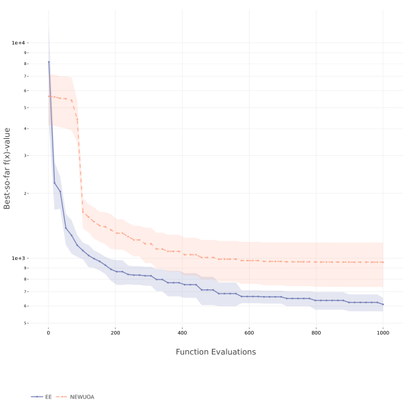
Figure 25: $f_{3}$, $D=40$. Here EXPLO2 is indicated by EE.

Figure 26: $f_{3}$, $D=40$. Here EXPLO2 is indicated by EE.

Figure 27: $f_{3}$, $D=40$. Here EXPLO2 is indicated by EE.

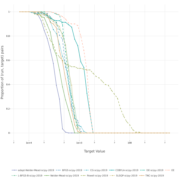
Figure 28: $f_{3}$, $D=40$. Here EXPLO2 is indicated by EE.

Figure 29: $f_{7}$, $D=20$. Here EXPLO2 is indicated by EE.

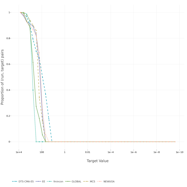
Figure 30: $f_{7}$, $D=20$. Here EXPLO2 is indicated by EE.

Figure 31: $f_{7}$, $D=20$. Here EXPLO2 is indicated by EE.

Figure 32: $f_{7}$, $D=40$. Here EXPLO2 is indicated by EE.

Figure 33: $f_{7}$, $D=40$. Here EXPLO2 is indicated by EE.

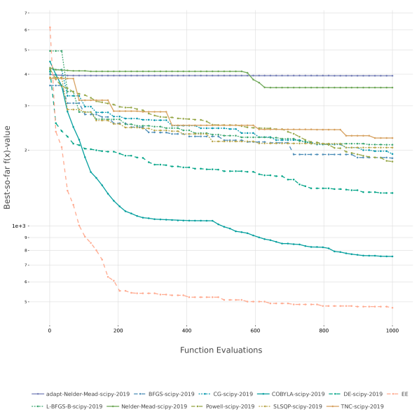
Figure 34: $f_{7}$, $D=40$. Here EXPLO2 is indicated by EE.

Figure 35: $f_{7}$, $D=40$. Here EXPLO2 is indicated by EE.

Figure 36: $f_{15}$, $D=20$. Here EXPLO2 is indicated by EE.

Figure 37: $f_{15}$, $D=20$. Here EXPLO2 is indicated by EE.

Figure 38: $f_{15}$, $D=20$. Here EXPLO2 is indicated by EE.

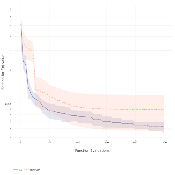
Figure 39: $f_{15}$, $D=40$. Here EXPLO2 is indicated by EE.

Figure 40: $f_{15}$, $D=40$. Here EXPLO2 is indicated by EE.

Figure 41: $f_{15}$, $D=40$. Here EXPLO2 is indicated by EE.

Figure 42: $f_{15}$, $D=40$. Here EXPLO2 is indicated by EE.

Figure 43: $f_{16}$, $D=20$. Here EXPLO2 is indicated by EE.

Figure 44: $f_{16}$, $D=20$. Here EXPLO2 is indicated by EE.

Figure 45: $f_{16}$, $D=20$. Here EXPLO2 is indicated by EE.

Figure 46: $f_{16}$, $D=40$. Here EXPLO2 is indicated by EE.

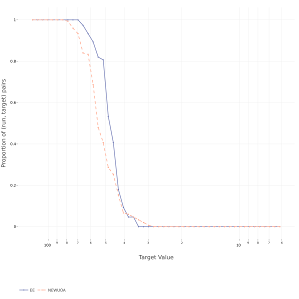
Figure 47: $f_{16}$, $D=40$. Here EXPLO2 is indicated by EE.

Figure 48: $f_{16}$, $D=40$. Here EXPLO2 is indicated by EE.

Figure 49: $f_{16}$, $D=40$. Here EXPLO2 is indicated by EE.

Figure 50: $f_{17}$, $D=20$. Here EXPLO2 is indicated by EE.

Figure 51: $f_{17}$, $D=20$. Here EXPLO2 is indicated by EE.

Figure 52: $f_{17}$, $D=20$. Here EXPLO2 is indicated by EE.

Figure 53: $f_{17}$, $D=40$. Here EXPLO2 is indicated by EE.

Figure 54: $f_{17}$, $D=40$. Here EXPLO2 is indicated by EE.

Figure 55: $f_{17}$, $D=40$. Here EXPLO2 is indicated by EE.

Figure 56: $f_{17}$, $D=40$. Here EXPLO2 is indicated by EE.

Figure 57: $f_{18}$, $D=20$. Here EXPLO2 is indicated by EE.

Figure 58: $f_{18}$, $D=20$. Here EXPLO2 is indicated by EE.

Figure 59: $f_{18}$, $D=20$. Here EXPLO2 is indicated by EE.

Figure 60: $f_{18}$, $D=40$. Here EXPLO2 is indicated by EE.

Figure 61: $f_{18}$, $D=40$. Here EXPLO2 is indicated by EE.

Figure 62: $f_{18}$, $D=40$. Here EXPLO2 is indicated by EE.

Figure 63: $f_{18}$, $D=40$. Here EXPLO2 is indicated by EE.

Figure 64: $f_{19}$, $D=20$. Here EXPLO2 is indicated by EE.

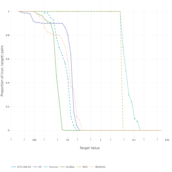
Figure 65: $f_{19}$, $D=20$. Here EXPLO2 is indicated by EE.

Figure 66: $f_{19}$, $D=20$. Here EXPLO2 is indicated by EE.

Figure 67: $f_{19}$, $D=40$

Figure 68: $f_{19}$, $D=40$. Here EXPLO2 is indicated by EE.

Figure 69: $f_{19}$, $D=40$. Here EXPLO2 is indicated by EE.

Figure 70: $f_{19}$, $D=40$. Here EXPLO2 is indicated by EE.

Appendix G Scaling of runtime with dimension

The expected runtime (ERT), used in the figures and tables, depends on a given target function value, $f_{\mathrm{t}}=f_{\mathrm{opt}}+\Delta f$, and is computed over all relevant trials as the number of function evaluations executed during each trial while the best function value did not reach $f_{\mathrm{t}}$, summed over all trials and divided by the number of trials that actually reached $f_{\mathrm{t}}$ (Hansen et al., 2012; Price, 1997). Statistical significance is tested with the rank-sum test for a given target $\Delta f_{\mathrm{t}}$ using, for each trial, either the number of needed function evaluations to reach $\Delta f_{\mathrm{t}}$ (inverted and multiplied by $-1$), or, if the target was not reached, the best $\Delta f$-value achieved, measured only up to the smallest number of overall function evaluations for any unsuccessful trial under consideration.

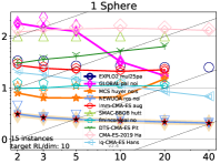
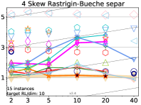
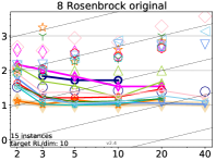
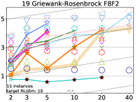
Figure 71: Expected running time ($\mathrm{ERT}$ in number of $f$-evaluations as $\log_{10}$ value) divided by dimension versus dimension. The target function value is chosen such that the best algorithm from BBOB 2009 just failed to achieve an $\mathrm{ERT}$ of $10\times\mathrm{DIM}$. Different symbols correspond to different algorithms given in the legend of $f_{1}$ and $f_{24}$. Light symbols give the maximum number of function evaluations from the longest trial divided by dimension. Black stars indicate a statistically better result compared to all other algorithms with $p<0.01$ and Bonferroni correction number of dimensions (six). Legend: $\circ$: EXPLO2 mul25par32lamLin, $\diamondsuit$: GLOBAL pal noiseless, $\star$: MCS huyer noiseless, $\triangledown$: NEWUOA ros noiseless, $\varhexagon$: lmm-CMA-ES auger noiseless, $\triangle$: SMAC-BBOB hutter noiseless, $\pentagon$: fmincon pal noiseless, $\downY$: DTS-CMA-ES Pitra, $\Diamond$: CMA-ES-2019 Hansen, $\triangleleft$: lq-CMA-ES Hansen

Appendix H Runtime distributions (ECDFs) per function: $D=20$

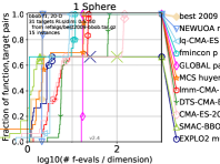
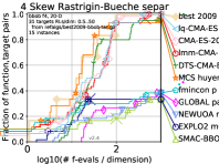
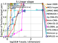
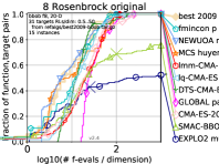
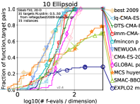
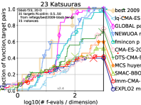
Figure 72: Empirical cumulative distribution of simulated (bootstrapped) runtimes, measured in number of objective function evaluations divided by dimension (FEvals/DIM) in dimension 20 and for those targets in $10^{[-8..2]}$ that have just not been reached by the best algorithm from BBOB 2009 in a given budget of $k$ $\times$ DIM, with $31$ different values of $k$ chosen equidistant in logscale within the interval $\{0.5,\dots,50\}$. Crosses ($\times$) indicate where experimental data ends and bootstrapping begins; algorithms are not comparable after this point. EXPLO2 used default options except for $n_{\parallel}=32$.

Appendix I Runtime distributions (ECDFs) per function: $D=40$

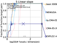
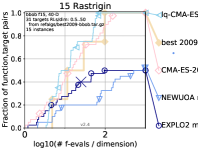
Figure 73: Empirical cumulative distribution of simulated (bootstrapped) runtimes, measured in number of objective function evaluations divided by dimension (FEvals/DIM) in dimension 40 and for those targets in $10^{[-8..2]}$ that have just not been reached by the best algorithm from BBOB 2009 in a given budget of $k$ $\times$ DIM, with $31$ different values of $k$ chosen equidistant in logscale within the interval $\{0.5,\dots,50\}$. Crosses ($\times$) indicate where experimental data ends and bootstrapping begins; algorithms are not comparable after this point. EXPLO2 used default options except for $n_{\parallel}=32$.

Appendix J Results from the large-scale BBOB suite

Figure 74: (Left panels) Bootstrapped empirical cumulative distribution of the number of objective function evaluations divided by dimension $D$ for structured multimodal functions $f_{15},\dots,f_{19}$ for $D\in\{20,40,80\}$. The targets are chosen from $10^{[-8\dots 2]}$ such that the best algorithm from BBOB 2009 just not reached them within a given budget of $k\times D$, with 31 different values of $k$ chosen equidistant in logscale within the interval $\{0.5,\dots,50\}$. As reference algorithm, the best algorithm from BBOB 2009 is shown as light thick line with diamond markers. Crosses ($\times$) indicate where experimental data ends and bootstrapping begins; algorithms are not comparable after this point. EXPLO2 used default options except for $n_{\parallel}=32$. (Right panels) As in the left panels, but for weakly structured multimodal functions $f_{20},\dots,f_{24}$.

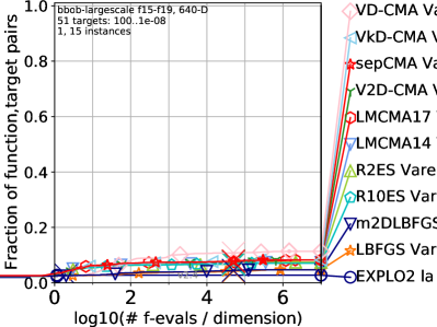
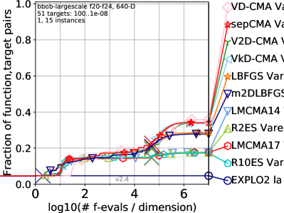
Figure 75: (Left panels) Bootstrapped empirical cumulative distribution of the number of objective function evaluations divided by dimension $D$ for structured multimodal functions $f_{15},\dots,f_{19}$ for $D\in\{160,320,640\}$. The targets are chosen from $10^{[-8\dots 2]}$ such that the best algorithm from BBOB 2009 just not reached them within a given budget of $k\times D$, with 31 different values of $k$ chosen equidistant in logscale within the interval $\{0.5,\dots,50\}$. As reference algorithm, the best algorithm from BBOB 2009 is shown as light thick line with diamond markers. Crosses ($\times$) indicate where experimental data ends and bootstrapping begins; algorithms are not comparable after this point. EXPLO2 used default options except for $n_{\parallel}=32$. (Right panels) As in the left panels, but for weakly structured multimodal functions $f_{20},\dots,f_{24}$.

Appendix K Result from the mixed-integer BBOB suite

Figure 76: Comparison of differential evolution, CMA-ES, and EXPLO2 on the mixed-integer version of the Rastrigin function $f_{15}$ for $D=20$. Crosses ($\times$) indicate where experimental data ends and bootstrapping begins; algorithms are not comparable after this point. EXPLO2 used default options except for $n_{\parallel}=32$.

Appendix L Source code for EXPLO2

NB. parfor loops are commented out in this code and replaced with for loops. This should be changed if not benchmarking.

function [x,y] = explo2(f,lb,ub,N,varargin)

% Optimizer based on a principled tradeoff between exploration (in the
% guise of optimal differential magnitude as diversity proxy) and
% exploitation (in the guise of a convenient radial basis function
% interpolation that is a proxy for the true objective).
%
% This function requires the optimization toolbox and optionally the
% parallel computing toolbox. (However, it should be relatively
% straightforward to port everything to Octave if needed.)
%
% This approach is only appropriate for functions whose evaluation is
% expensive: as such, it seeks to compete with, e.g., metaheuristics,
% deterministic algorithms such as DIRECT, MCS, or ADC; and other
% surrogate-assisted techniques. The key scaling desiderata are low
% function evaluation budget and high dimension.
%
% By default, execution is serial; this and other options can be set in a
% final input (see below) for which defaults are provided.
%
% Inputs:
%     f,    a handle to a scalar function with column input/output. It is
%           assumed that f takes arguments of the same size as lb/ub
%     lb,   a vector of lower bounds on the domain of f (must be finite)
%     ub,   a vector of upper bounds on the domain of f (must be finite)
%     N,Ψthe number of function evaluations
%     (optional),  options structure with fields including
%         n_parallel,Ψnumber of parallel workers
%         n_sample,     number of points for downsampling
%         n_explore,Ψnumber of points for computing exploreRange
%         n_tries,      number of tries for optimizing surrogate
%         lambda,       regularization parameter for explore-exploit trade
%         init,         initial evaluation point selection strategy
%     See the default options for detailed explanations. The init option
%     must be one of ’uniform’, ’near_corners’, or ’corners’.
%
% Outputs:
%     x,Ψevaluation points (array of size [dim,N])
%     y,Ψcorresponding function values
%
% Examples:
%     Rastrigin function
%         f = @(x) 10*numel(x)+x(:)’*x(:)-10*sum(cos(2*pi*x(:)));
%         dim = 2;
%         lb = -5.12*ones(dim,1);
%         ub = 5.12*ones(dim,1);
%     Rosenbrock function
%         f = @(x) sum(100*(x(2:end)-x(1:end-1).^2).^2+(1-x(1:end-1)).^2);
%         dim = 2;
%         lb = -1*ones(dim,1);
%         ub = 3*ones(dim,1);
%     Himmelblau function (dim = 2 only)
%         f = @(x) (x(1)^2+x(2)-11)^2+(x(1)+x(2)^2-7)^2;
%         lb = -5*ones(2,1);
%         ub = 5*ones(2,1);
% NB. Using an anonymous function handle as in these examples causes memory
% to get dragged along during broadcasting. In practice (vs testing),
% however, a function handle should not be anonymous, though likely it
% wouldn’t be anyway for this optimization technique to make sense. See
% https://www.mathworks.com/matlabcentral/answers/339728
%
% AKA eeOptimize.m
%
% Last modified 20210727 by Steve Huntsman
%
% Copyright (c) 2021, 2022, Systems & Technology Research. All rights reserved.


%% %% %% %% %% %% HERE FOLLOW ~130 LINES OF PRELIMINARIES %% %% %% %% %% %%

%% Preliminary checks (except for options, which are treated below)
narginchk(4,5); % at most one extra argument, which must be options
if ~isa(f,’function_handle’), error(’f must be a function handle’); end
% Bounds
if ~ismatrix(lb), error(’lower bound not in matrix form’); end
if ~ismatrix(ub), error(’upper bound not in matrix form’); end
if any(size(lb)~=size(ub)), error(’lower/upper bound size mismatch’); end
if any(~isreal(lb(:))), error(’lower bound not real’); end
if any(~isreal(ub(:))), error(’upper bound not real’); end
if any(~isfinite(lb(:))), error(’lower bound not finite’); end
if any(~isfinite(ub(:))), error(’upper bound not finite’); end
if any(lb>ub), error(’lower bound must be less than upper bound’); end
lb = lb(:);
ub = ub(:);
dim = numel(lb);
% Number of function evaluations
if ~isscalar(N), error(’N must be scalar’); end
if ~isreal(N), error(’N must be real’); end
if ~isfinite(N), error(’N must be finite’); end
if N <= dim, error(’N must be > dim’); end
if N ~= round(N), error(’N must be integral’); end

%% Default options
% Number of parallel workers, set to 1 by default to avoid parfor
defaultOptions.n_parallel = 1;
% Number of points for downsampling. This is necessary to have constant
% runtime per loop iteration. With this in mind, we pick points with
% greatest interpolation error and least values: see main loop.
defaultOptions.n_sample = 100;
% Number of points for computing exploreRange. This is necessary because
% the simple far-field asymptotic behavior does not yield an adequate
% approximation. If n_explore >= 2^dim, then only the corners of the
% bounding box are used below.
defaultOptions.n_explore = 100;
% Number of trials for optimizing surrogate (starting from uniformly random
% location). Quoting [*]:
%     "In problems where the cost of fitting and evaluating a surrogate is
%     much less than the cost of evaluating the true objective function or
%     surrogates is a viable approach to find multiple optima."
% [*] Villanueva, Diane, et al. "Locating multiple candidate designs with
% surrogate-based optimization." WCSMO (2013).
defaultOptions.n_tries = 3;
% Regularization parameter for explore-exploit tradeoff. Alternatives might
% be any sigmoidal function decreasing from 1 at 0 to 0 at 1, e.g.,
%     bf = bumpfun(0,1,0); lambda = arrayfun(bf,linspace(0,1,N));
% The bumpfun function is available from Steve Huntsman.
%
% Here, we use the following decidedly non-sigmoidal function:
% exp(-(log(2)/log(delta))*log(1-t)) takes the value 1/2 at 1-delta. Taking
% delta = 1/2 yields an affine function, which we have used. Assuming that
% N scales like C*dim, taking delta = 1/dim is also natural (and commented
% out).
delta = 1/2;    % corresponds to defaultOptions.lambda = 1-t
% if N/dim > 1
%     delta = 1/dim;
% else
%     delta = 1/sqrt(N);
% end
defaultOptions.lambda = exp(-(log(2)/log(delta))*log(linspace(1,0,N)));
% Initial evaluation point selection strategy
defaultOptions.init = ’uniform’;

%% Set options, using defaults except as specified via input
availableOptions = fieldnames(defaultOptions);  % ignore anything else
if nargin == 5
    options = varargin{end};
    if ~isstruct(options), error(’options must be struct’); end
    if numel(options) > 1
        error(’options must have a single entry (multiple fields are OK)’);
    end
    opts = fieldnames(options);
    % Ignore any fields not in availableOptions; check all options below
    ind = ismember(availableOptions,opts);
    for j = 1:numel(availableOptions)
        opt = availableOptions{j};
        if ind(j)
            % Option is specified via input, so do NOT use the default
            eval([opt,’ = options.’,opt,’;’]);  % tolerable use of eval
        else
            % Option is not specified via input, so use the default
            eval([opt,’ = defaultOptions.’,opt,’;’]);   % tolerable use of eval
        end
    end
else
    % Use default options
    for j = 1:numel(availableOptions)
        opt = availableOptions{j};
        eval([opt,’ = defaultOptions.’,opt,’;’]);   % tolerable use of eval
    end
end

%% Preliminary checks for options--mostly boilerplate
% n_parallel
if ~isscalar(n_parallel), error(’n_parallel must be scalar’); end
if ~isreal(n_parallel), error(’n_parallel must be real’); end
if ~isfinite(n_parallel), error(’n_parallel must be finite’); end
if n_parallel > 128, error(’n_parallel must be <= 128’); end  % ad hoc
if n_parallel ~= round(n_parallel), error(’n_parallel must be integral’); end
% n_sample
if ~isscalar(n_sample), error(’n_sample must be scalar’); end
if ~isreal(n_sample), error(’n_sample must be real’); end
if ~isfinite(n_sample), error(’n_sample must be finite’); end
if n_sample < 16, error(’n_sample must be >= 16’); end  % ad hoc
if n_sample ~= round(n_sample), error(’n_sample must be integral’); end
% n_explore
if ~isscalar(n_explore), error(’n_explore must be scalar’); end
if ~isreal(n_explore), error(’n_explore must be real’); end
if ~isfinite(n_explore), error(’n_explore must be finite’); end
if n_explore < 16, error(’n_explore must be >= 16’); end  % ad hoc
if n_explore ~= round(n_explore), error(’n_explore must be integral’); end
% n_tries
if ~isscalar(n_tries), error(’n_tries must be scalar’); end
if ~isreal(n_tries), error(’n_tries must be real’); end
if ~isfinite(n_tries), error(’n_tries must be finite’); end
if n_tries < 0, error(’n_tries must be >= 0’); end
if n_tries ~= round(n_tries)
    error(’n_tries must be integral’);
end
% lambda
% NB. MATLAB’s static analyzer needlessly worries about this being defined
if ~ismatrix(lambda), error(’lambda not matrix’); end
if numel(lambda) ~= N
    warning(’numel(lambda) ~= N; truncating or padding with zeros’);
    if numel(lambda) < N
        lambda = [lambda(:)’,zeros(1,N-numel(lambda))];
    else
        lambda = lambda(1:N);
    end
end
if ~all(isfinite(lambda)&isreal(lambda))
    error(’lambda must be real and finite’);
end
if any((lambda<0)|(lambda>1))
    warning(’lambda not between 0 and 1’);
end
% initialization
initStrategies = {’uniform’,’near_corners’,’corners’};
if ~ischar(init), error(’init must be a char array’); end
ind = ismember(initStrategies,init);
if nnz(ind) ~= 1
    error(’init must be ’’uniform’’, ’’near_corners’’, or ’’corners’’’);
end

%% %% %% %% %% %% ACTUAL SUBSTANTIVE CODE BEGINS HERE %% %% %% %% %% %%

%% Initial locations for function evaluations
% There are three available strategies:
%     ’uniform’,        uniform random sampling;
%     ’near_corners’,Ψuniform random sampling in small boxes inscribed in
%                       bounding box corners;
%     ’corners’,        deterministic sampling at bounding box corners
% ’uniform’ has all the usual advantages and disadvantages, whereas
% ’corners’ has the advantage of determinism and the feature of quickly
% putting pressure on the interior of the bounding box, i.e., it
% effectively foreshortens the exploration phase. ’near_corners’ has the
% advantage of avoiding degeneracies and artifacts that ’corners’ can
% cause, particularly on test problems with symmetry. Both ’near_corners’
% and ’corners’ take points near/at lb and corners at locations from it
% that are parallel to the coordinate axes.
N0 = dim+1; % we need this many initial points for general position stuff
if strcmp(init,’uniform’)
    x = diag(ub-lb)*rand(dim,N0)+diag(lb)*ones(dim,N0);
    % This assertion fails with measure zero--pretty safe bet...
    ux = unique(x’,’rows’)’;
    assert(size(ux,2)==size(x,2),’duplicate inputs!’);Ψ% ...check anyway
elseif strcmp(init,’near_corners’)
    extent = ub-lb;
    margin = .1;
    x = [lb,lb*ones(1,dim)+diag(extent)*(1-margin)]...
        +margin*diag(extent)*rand(dim,dim+1);
elseif strcmp(init,’corners’)   % deterministic
    extent = ub-lb;
    x = [lb,lb*ones(1,dim)+diag(extent)];
else
    error(’bad init option: this was supposedly already checked!’);
end

%% Finish initializing x and y
x = [x,nan(dim,N-N0)];
y = nan(1,N);
if n_parallel > 1
    for n = 1:N0    % use parfor in practice
        y(n) = f(x(:,n));   % broadcast overhead OK in practice
    end
else
    for n = 1:N0
        y(n) = f(x(:,n));
    end
end

%% Initialize t
% Using t >= [positive cutoff] would be problematic because of clustering
% that drives the cutoff to large values. So we work in the limit t -> 0.
% However, using the analytical results of the limit typically gives
% fmincon problems, so we avoid that below.
t = sqrt(eps);

%% Initialize relative error
relErr = nan(1,N);

%% For estimating range of explore function in main loop
lbub = [lb,ub];
if n_explore >= 2^dim
    bits = double(dec2bin((1:2^dim)-1,dim))’-48;    % ASCII hack
    indCorners = (1:dim)’*ones(1,2^dim)+dim*bits;
end

%% Main loop
n = N0+1;
while n < N
    %%
    disp([’optimizer: function evaluation ’,num2str(n),’/’,num2str(N)]);

    %% Downsample
    % We pick points with greatest interpolation error and least values.
    % Provided that lambda appropriately decreases to move from exploration
    % to exploitation, incorporating it here tends to explore boundaries
    % more at first; later, it avoids "superfluous" minima
    n_err = round(n_sample*min(1,lambda(n)/lambda(1)));
    if n > n_sample
        [~,ind_err] = sort(relErr,’descend’);Ψ% N0 NaNs at first is OK
        topErrors = ind_err(1:n_err);
        % Get indices for least values of y that aren’t in topErrors
        [~,ind_y] = sort(y);
        leastValues = setdiff(ind_y,topErrors,’stable’);
        ind_sample = [topErrors,leastValues(1:(n_sample-n_err))];
    else
        ind_sample = 1:(n-1);
    end
    x_sample = x(:,ind_sample);
    y_sample = y(ind_sample);

    %% Update d, Z, w
    d = squareform(pdist(x_sample’));
    Z = exp(-t*d);
    w = Z\ones(size(Z,1),1);

    %% Exploit using Laplacian RBF interpolation
    interpDist = @(xn) vecnorm(x_sample-xn*ones(1,size(x_sample,2)));
    zeta = @(xn) exp(-t*interpDist(xn))’;
    interpCoeff = y_sample/Z;
    exploit = @(xn) interpCoeff*zeta(xn);   % surrogate (vs proxy below)
    exploitRange = max(y_sample)-min(y_sample);
    exploitRange = exploitRange+(exploitRange==0);  % for safety

    %% Sequentially select n_parallel points for parallel evaluation later
    for j = 1:n_parallel

        %% Explore using change in magnitude
        explore = @(xn) ((1-zeta(xn)’*w)^2)/(1-zeta(xn)’/Z*zeta(xn));

        %% Estimate range of explore by sampling corners
        warning off;    % explore may be inaccurate; don’t remind ourselves
        if n_explore < 2^dim
            % Sample because there are too many corners. Don’t worry about
            % possible duplicates--these are unlikely to matter much
            exploreCorners = nan(1,n_explore);
            for k = 1:n_explore
                exploreCorners(k) = explore(lbub((randi(2,dim,1)-1)*dim+(1:dim)’));
            end
        else
            % No point in sampling: just evaluate at all corners
            exploreCorners = nan(1,2^dim);
            for k = 1:2^dim
                exploreCorners(k) = explore(lbub(indCorners(:,k)));
            end
        end
        exploreRange = max(exploreCorners);
        exploreRange = exploreRange+(exploreRange==0);  % for safety
        warning on;

        %% Well-behaved surrogate that incorporates exploration
        % Normalize explore and exploit to be approximately in unit
        % interval. The minus sign is because we want to minimize both
        % terms.
        surrogate = @(xn) exploit(xn)/exploitRange...
            -lambda(n)*explore(xn)/exploreRange;

        %% New evaluation point is local optimum of proxy objective
        optopt = optimoptions(@fmincon,’Display’,’off’);   % no stdout
        try
            warning off;    % can be inaccurate; don’t remind ourselves
            surrogateOptimum = Inf;
            % Do not bother with parfor on the surrogate
            for k = 1:n_tries
                x0 = diag(ub-lb)*rand(dim,1)+diag(lb)*ones(dim,1);  % uniform
                [x_sur,y_sur] = ...
                    fmincon(surrogate,x0,[],[],[],[],lb,ub,[],optopt);
                if y_sur < surrogateOptimum
                    xn = x_sur;
                    surrogateOptimum = y_sur;
                else
                    break;  % stop trying as soon as there’s no improvement
                end
            end
            warning on;
        catch
            % We don’t expect this to happen...
            disp(’fmincon failed; evaluating at uniformly random point’);
            pause(.01);
            x0 = diag(ub-lb)*rand(dim,1)+diag(lb)*ones(dim,1);  % uniform
            xn = x0;
        end

        %% Update x_sample
        x_sample = [x_sample,xn];

        %% Update d, Z, w
        d = squareform(pdist(x_sample’));
        Z = exp(-t*d);
        w = Z\ones(size(Z,1),1);

        %% Update function handles that feed into explore
        interpDist = @(xn) vecnorm(x_sample-xn*ones(1,size(x_sample,2)));
        zeta = @(xn) exp(-t*interpDist(xn))’;

    end

    %% Memorialize and evaluate new points (in parallel if n_parallel > 1)
    % Unfortunately, running parfor inside a loop is slow, since the
    % parallel pool must be reinitialized on each iteration. There does not
    % seem to be any way around this, though.
    x(:,n-1+(1:n_parallel)) = x_sample(:,(end-n_parallel+1):end);
    temp_y = nan(1,n_parallel);Ψ% this placeholder is needed for parfor
    if n_parallel > 1
        for j = 1:n_parallelΨ% use parfor in practice
            temp_y(j) = f(x(:,n-1+j));Ψ% Broadcast overhead OK in practice
        end
    else
        temp_y = f(x(:,n));
    end
    y(n-1+(1:n_parallel)) = temp_y;

    %% Get relative errors of interpolation for downsampling
    relErr = nan(1,n-1+n_parallel);
    for j = 1:numel(relErr)
        relErr(j) = abs(1-exploit(x(:,j))/y(j));
    end

    %% Update n
    n = n+n_parallel;

end

Appendix M Source code for benchmarking

M.1 EXPLO2 version for COCO interface

function [x,y] = coco_explo2 (problem, ...
    lower_bounds, upper_bounds, num_integer_vars, num_constraints, budget)

% cf. my_optimizer.m

f = @(x) cocoEvaluateFunction(problem,x);
lb = lower_bounds(:);
ub = upper_bounds(:);
N = budget;
%% EXPLO2 options (don’t comment all of these out)
options.n_parallel = 32;             % default: 1
% options.n_sample = 100;             % default: 100
% options.n_explore = 100;            % default: 100
% options.n_tries = 3;                % default: 3
% options.lambda = linspace(1,0,N);   % default: a bit complicated

% dim = cocoProblemGetDimension(problem);
% B = N;
% lam = [];
% while B > dim
%     B = floor(B/2);
%     lam = [lam,linspace(0,1,B)];
% end
% lam = [lam,linspace(0,1,N-numel(lam))];
% lam = fliplr(lam);
% options.lambda = lam;

% NN = double(N);
% lam = -log(linspace(1/NN,1,NN));
% options.lambda = lam;

% dim = cocoProblemGetDimension(problem);
% B = double(N);
% lam = [];
% while B > dim
%     B = floor(B/2);
%     lam = [lam,-log(linspace(1/B,1,B))];
% end
% lam = [lam,-log(linspace(1/(double(N)-numel(lam)),1,double(N)-numel(lam)))];
% options.lambda = double(lam);

dim = cocoProblemGetDimension(problem);
options.lambda = [ones(1,N-dim),linspace(1,0,dim)];

% options.init = ’uniform’;           % default: uniform
%%
[x,y] = explo2(f,lb,ub,N,options);

M.2 Benchmarking script

% COCO benchmarking of EXPLO2
%
% [From COCO documentation: This example experiment allows also for easy
% implementation of independent restarts by simply increasing
% NUM_OF_INDEPENDENT_RESTARTS. To make this effective, the algorithm should
% have at least one more stopping criterion than just a maximal budget.]
%
more off; % to get immediate output in Octave

%%%%%%%%%%%%%%%%%%%%%%%%%
% Experiment Parameters %
%%%%%%%%%%%%%%%%%%%%%%%%%
BUDGET_MULTIPLIER = 25; % algorithm runs for BUDGET_MULTIPLIER*dimension funevals
NUM_OF_INDEPENDENT_RESTARTS = 1e9; % max. number of independent algorithm
% restarts; if >0, make sure that the
% algorithm is not always doing the same thing
% in each run (which is typically trivial for
% randomized algorithms)

%%%%%%%%%%%%%%%%%%%%%%%%%
% Prepare Experiment    %
%%%%%%%%%%%%%%%%%%%%%%%%%

% choose a test suite and a matching logger, for
% example one of the following:
%
% bbob               24 unconstrained noiseless single-objective functions
% bbob-biobj         55 unconstrained noiseless bi-objective functions
% [bbob-biobj-ext     92 unconstrained noiseless bi-objective functions]
% bbob-largescale    24 unconstrained noiseless single-objective functions in large dimensions
% [bbob-constrained* 48 constrained noiseless single-objective functions]
% bbob-mixint        24 unconstrained noiseless single-objective functions with mixed-integer variables
% bbob-biobj-mixint  92 unconstrained noiseless bi-objective functions with mixed-integer variables
%
% Suites with a star are partly implemented but not yet fully supported.
%
suite_name = ’bbob’;
observer_name = ’bbob’;
observer_options = strcat(’result_folder: EXPLO2_on_’, ...
    suite_name, ...
    [’ algorithm_name: EXPLO2 ’...
    ’ algorithm_info: EXPLO2 ’]);

% initialize suite and observer with default options,
% to change the default, see
% http://numbbo.github.io/coco-doc/C/#suite-parameters and
% http://numbbo.github.io/coco-doc/C/#observer-parameters
% for details.
% suite = cocoSuite(suite_name, ’’, ’’);
% observer = cocoObserver(observer_name, observer_options);
    suite_options = [’dimensions: 20 function_indices: 15-19’];
    suite = cocoSuite(suite_name, ’’, suite_options);
    observer = cocoObserver(observer_name, observer_options);

    % set log level depending on how much output you want to see, e.g. ’warning’
    % for fewer output than ’info’.
    cocoSetLogLevel(’info’);

    % keep track of problem dimension and #funevals to print timing information:
    printeddim = 1;
    doneEvalsAfter = 0; % summed function evaluations for a single problem
    doneEvalsTotal = 0; % summed function evaluations per dimension
    printstring = ’\n’; % store strings to be printed until experiment is finished

    %%%%%%%%%%%%%%%%%%%%%%%%%
    % Run Experiment        %
    %%%%%%%%%%%%%%%%%%%%%%%%%
    while true
        % get next problem and dimension from the chosen suite:
        problem = cocoSuiteGetNextProblem(suite, observer);
        if ~cocoProblemIsValid(problem)
            break;
        end
        dimension = cocoProblemGetDimension(problem);

        % printing
        if printeddim < dimension
          if printeddim > 1
            elapsedtime = toc;
            printstring = strcat(printstring, ...
                sprintf(’   COCO TIMING: dimension %d finished in %e seconds/evaluation\n’, ...
                printeddim, elapsedtime/double(doneEvalsTotal)));
            tic;
          end
          doneEvalsTotal = 0;
          printeddim = dimension;
          tic;
        end

        %
        lower_bounds = cocoProblemGetSmallestValuesOfInterest(problem);
        upper_bounds = cocoProblemGetLargestValuesOfInterest(problem);
        num_integer_vars = cocoProblemGetNumberOfIntegerVariables(problem);
        if num_integer_vars, warning(’integer vars’); end
        num_constraints = cocoProblemGetNumberOfConstraints(problem);
        if num_constraints, warning(’constraints’); end
        dimension = cocoProblemGetDimension(problem);
        budget = BUDGET_MULTIPLIER*dimension;

        rng(’default’); % for reproducibility at every stage
        [x,y] = coco_explo2(problem, lower_bounds, upper_bounds, ...
            num_integer_vars, num_constraints, budget);

    doneEvalsTotal = budget;
    end

    elapsedtime = toc;
    printstring = strcat(printstring, ...
        sprintf(’   COCO TIMING: dimension %d finished in %e seconds/evaluation\n’, ...
        printeddim, elapsedtime/double(doneEvalsTotal)));
    fprintf(printstring);

    cocoObserverFree(observer);
    cocoSuiteFree(suite);

References

- Akimoto et al. (2014) Akimoto, Y., Auger, A., and Hansen, N. Comparison-based natural gradient optimization in high dimension. In Proceedings of the 2014 Annual Conference on Genetic and Evolutionary Computation, pp. 373–380, 2014.
- Alaee et al. (2020) Alaee, S., Kamgar, K., and Keogh, E. Matrix profile xxii: exact discovery of time series motifs under dtw. arXiv preprint arXiv:2009.07907, 2020.
- Alpak et al. (2013) Alpak, F. O., Vink, J. C., Gao, G., and Mo, W. Techniques for effective simulation, optimization, and uncertainty quantification of the in-situ upgrading process. Journal of Unconventional Oil and Gas Resources, 3:1–14, 2013.
- Andoni et al. (2018) Andoni, A., Indyk, P., and Razenshteyn, I. Approximate nearest neighbor search in high dimensions. In Proceedings of the International Congress of Mathematicians: Rio de Janeiro 2018, pp. 3287–3318. World Scientific, 2018.
- Assent (2012) Assent, I. Clustering high dimensional data. Wiley Interdisciplinary Reviews: Data Mining and Knowledge Discovery, 2(4):340–350, 2012.
- Audet & Hare (2017) Audet, C. and Hare, W. Derivative-free and blackbox optimization. 2017.
- Auger et al. (2013) Auger, A., Brockhoff, D., and Hansen, N. Benchmarking the local metamodel cma-es on the noiseless bbob’2013 test bed. In Proceedings of the 15th annual conference companion on Genetic and evolutionary computation, pp. 1225–1232, 2013.
- Bajer et al. (2019) Bajer, L., Pitra, Z., Repickỳ, J., and Holeňa, M. Gaussian process surrogate models for the cma evolution strategy. Evolutionary computation, 27(4):665–697, 2019.
- Bischl et al. (2014) Bischl, B., Wessing, S., Bauer, N., Friedrichs, K., and Weihs, C. Moi-mbo: multiobjective infill for parallel model-based optimization. In International Conference on Learning and Intelligent Optimization, pp. 173–186. Springer, 2014.
- Björkman & Holmström (2000) Björkman, M. and Holmström, K. Global optimization of costly nonconvex functions using radial basis functions. Optimization and Engineering, 1(4):373–397, 2000.
- Bonnet et al. (2021) Bonnet, G., Gusakova, A., Thäle, C., and Zaporozhets, D. Sharp inequalities for the mean distance of random points in convex bodies. Advances in Mathematics, 386:107813, 2021.
- Booker et al. (1999) Booker, A. J., Dennis, J. E., Frank, P. D., Serafini, D. B., Torczon, V., and Trosset, M. W. A rigorous framework for optimization of expensive functions by surrogates. Structural optimization, 17(1):1–13, 1999.
- Brockhoff (2015) Brockhoff, D. Comparison of the matsumoto library for expensive optimization on the noiseless black-box optimization benchmarking testbed. In 2015 IEEE Congress on Evolutionary Computation (CEC), pp. 2026–2033. IEEE, 2015.
- Buhmann (2003) Buhmann, M. D. Radial basis functions: theory and implementations, volume 12. Cambridge, 2003.
- Bunch et al. (2020) Bunch, E., Dickinson, D., Kline, J., and Fung, G. Practical applications of metric space magnitude and weighting vectors. arXiv preprint arXiv:2006.14063, 2020.
- Chatzilygeroudis et al. (2021) Chatzilygeroudis, K., Cully, A., Vassiliades, V., and Mouret, J.-B. Quality-diversity optimization: a novel branch of stochastic optimization. In Black Box Optimization, Machine Learning, and No-Free Lunch Theorems, pp. 109–135. Springer, 2021.
- Chenhan et al. (2017) Chenhan, D. Y., March, W. B., and Biros, G. An parallel fast direct solver for kernel matrices. In 2017 IEEE International Parallel and Distributed Processing Symposium (IPDPS), pp. 886–896. IEEE, 2017.
- Clerc (2018) Clerc, M. ITERATIVE OPTIMISATION : THE QUESTIONABLE BALANCE MANTRA. working paper or preprint, November 2018. URL https://hal.archives-ouvertes.fr/hal-01930529.
- Clerc (2019) Clerc, M. Iterative Optimizers: Difficulty Measures and Benchmarks. John Wiley & Sons, 2019.
- Csendes (1988) Csendes, T. Nonlinear parameter estimation by global optimization-efficiency and reliability. Acta Cybernetica, 8(4):361–370, 1988.
- Csendes et al. (2008) Csendes, T., Pál, L., Sendin, J. O. H., and Banga, J. R. The global optimization method revisited. Optimization Letters, 2(4):445–454, 2008.
- Datar et al. (2004) Datar, M., Immorlica, N., Indyk, P., and Mirrokni, V. S. Locality-sensitive hashing scheme based on p-stable distributions. In Proceedings of the twentieth annual symposium on Computational geometry, pp. 253–262, 2004.
- Doerr et al. (2018) Doerr, C., Wang, H., Ye, F., van Rijn, S., and Bäck, T. Iohprofiler: A benchmarking and profiling tool for iterative optimization heuristics. arXiv preprint arXiv:1810.05281, 2018.
- Elhara et al. (2019) Elhara, O., Varelas, K., Nguyen, D., Tusar, T., Brockhoff, D., Hansen, N., and Auger, A. Coco: the large scale black-box optimization benchmarking (bbob-largescale) test suite. arXiv preprint arXiv:1903.06396, 2019.
- Eriksson et al. (2019) Eriksson, D., Pearce, M., Gardner, J., Turner, R. D., and Poloczek, M. Scalable global optimization via local Bayesian optimization. In Advances in Neural Information Processing Systems, pp. 5496–5507, 2019. URL http://papers.nips.cc/paper/8788-scalable-global-optimization-via-local-bayesian-optimization.pdf.
- Fister et al. (2019) Fister, I., Iglesias, A., Galvez, A., Del Ser, J., Osaba, E., Fister Jr, I., Perc, M., and Slavinec, M. Novelty search for global optimization. Applied Mathematics and Computation, 347:865–881, 2019.
- Fontaine et al. (2020) Fontaine, M. C., Togelius, J., Nikolaidis, S., and Hoover, A. K. Covariance matrix adaptation for the rapid illumination of behavior space. In Proceedings of the 2020 genetic and evolutionary computation conference, pp. 94–102, 2020.
- Frazier (2018) Frazier, P. I. Bayesian optimization. In Recent Advances in Optimization and Modeling of Contemporary Problems, pp. 255–278. INFORMS, 2018.
- Gao et al. (2017) Gao, G., Vink, J. C., Chen, C., El Khamra, Y., and Tarrahi, M. Distributed gauss-newton optimization method for history matching problems with multiple best matches. Computational Geosciences, 21(5):1325–1342, 2017.
- Gao et al. (2020) Gao, G., Wang, Y., Vink, J., Wells, T., and Saaf, F. Distributed quasi-newton derivative-free optimization method for optimization problems with multiple local optima. In ECMOR XVII, volume 2020, pp. 1–22. European Association of Geoscientists & Engineers, 2020.
- Gao et al. (2021) Gao, G., Florez, H., Vink, J. C., Wells, T. J., Saaf, F., and Blom, C. P. Performance analysis of trust region subproblem solvers for limited-memory distributed bfgs optimization method. Frontiers in Applied Mathematics and Statistics, 7:673412, 2021.
- Gimperlein & Goffeng (2021) Gimperlein, H. and Goffeng, M. On the magnitude function of domains in euclidean space. American Journal of Mathematics, 143(3):to appear, 2021.
- Guillot & Rajaratnam (2012) Guillot, D. and Rajaratnam, B. Retaining positive definiteness in thresholded matrices. Linear algebra and its applications, 436(11):4143–4160, 2012.
- Gurvich & Vyalyi (2012) Gurvich, V. and Vyalyi, M. Characterizing (quasi-) ultrametric finite spaces in terms of (directed) graphs. Discrete Applied Mathematics, 160(12):1742–1756, 2012.
- Gutmann (2001) Gutmann, H.-M. A radial basis function method for global optimization. Journal of global optimization, 19(3):201–227, 2001.
- Haftka et al. (2016) Haftka, R. T., Villanueva, D., and Chaudhuri, A. Parallel surrogate-assisted global optimization with expensive functions–a survey. Structural and Multidisciplinary Optimization, 54(1):3–13, 2016.
- Hansen (2019) Hansen, N. A global surrogate assisted cma-es. In Proceedings of the Genetic and Evolutionary Computation Conference, pp. 664–672, 2019.
- Hansen et al. (2003) Hansen, N., Müller, S. D., and Koumoutsakos, P. Reducing the time complexity of the derandomized evolution strategy with covariance matrix adaptation (cma-es). Evolutionary computation, 11(1):1–18, 2003.
- Hansen et al. (2009) Hansen, N., Finck, S., Ros, R., and Auger, A. Real-parameter black-box optimization benchmarking 2009: Noiseless functions definitions. Technical Report RR-6829, INRIA, 2009. URL http://coco.lri.fr/downloads/download15.03/bbobdocfunctions.pdf. Updated February 2010.
- Hansen et al. (2010) Hansen, N., Auger, A., Ros, R., Finck, S., and Pošík, P. Comparing results of 31 algorithms from the black-box optimization benchmarking bbob-2009. In Proceedings of the 12th annual conference companion on Genetic and evolutionary computation, pp. 1689–1696, 2010.
- Hansen et al. (2012) Hansen, N., Auger, A., Finck, S., and Ros, R. Real-parameter black-box optimization benchmarking 2012: Experimental setup. Technical report, INRIA, 2012. URL http://coco.gforge.inria.fr/bbob2012-downloads.
- Hansen et al. (2016a) Hansen, N., Auger, A., Brockhoff, D., Tušar, D., and Tušar, T. COCO: Performance assessment. ArXiv e-prints, arXiv:1605.03560, 2016a.
- Hansen et al. (2016b) Hansen, N., Tušar, T., Mersmann, O., Auger, A., and Brockhoff, D. COCO: The experimental procedure. ArXiv e-prints, arXiv:1603.08776, 2016b.
- Hansen et al. (2021) Hansen, N., Auger, A., Ros, R., Mersmann, O., Tušar, T., and Brockhoff, D. Coco: A platform for comparing continuous optimizers in a black-box setting. Optimization Methods and Software, 36(1):114–144, 2021.
- Horn & Johnson (2012) Horn, R. A. and Johnson, C. R. Matrix Analysis. Cambridge, 2012.
- Huntsman (2020) Huntsman, S. Fast markov chain monte carlo algorithms via lie groups. In International Conference on Artificial Intelligence and Statistics, pp. 2841–2851, 2020.
- Huntsman (2021) Huntsman, S. Sampling and statistical physics via symmetry. In Barbaresco, F. and Nielsen, F. (eds.), Joint Structures and Common Foundation of Statistical Physics, Information Geometry and Inference for Learning. Springer, 2021.
- Hutter et al. (2013) Hutter, F., Hoos, H., and Leyton-Brown, K. An evaluation of sequential model-based optimization for expensive blackbox functions. In Proceedings of the 15th annual conference companion on Genetic and evolutionary computation, pp. 1209–1216, 2013.
- Huyer & Neumaier (1999) Huyer, W. and Neumaier, A. Global optimization by multilevel coordinate search. Journal of Global Optimization, 14(4):331–355, 1999.
- Jones & Martins (2021) Jones, D. R. and Martins, J. R. The direct algorithm: 25 years later. Journal of Global Optimization, 79(3):521–566, 2021.
- Kaluža et al. (2010) Kaluža, B., Mirchevska, V., Dovgan, E., Luštrek, M., and Gams, M. An agent-based approach to care in independent living. In International Joint Conference on Ambient Intelligence, pp. 177–186. Springer, 2010.
- Kern et al. (2006) Kern, S., Hansen, N., and Koumoutsakos, P. Local meta-models for optimization using evolution strategies. In Parallel Problem Solving from Nature-PPSN IX, pp. 939–948. Springer, 2006.
- Khan (2018) Khan, N. A parallel implementation of the covariance matrix adaptation evolution strategy. arXiv preprint arXiv:1805.11201, 2018.
- Koch et al. (2018) Koch, P., Golovidov, O., Gardner, S., Wujek, B., Griffin, J., and Xu, Y. Autotune: A derivative-free optimization framework for hyperparameter tuning. In Proceedings of the 24th ACM SIGKDD International Conference on Knowledge Discovery & Data Mining, pp. 443–452, 2018.
- Krause & Golovin (2014) Krause, A. and Golovin, D. Submodular function maximization. Tractability, 3:71–104, 2014.
- Lehman & Stanley (2011) Lehman, J. and Stanley, K. O. Abandoning objectives: Evolution through the search for novelty alone. Evolutionary computation, 19(2):189–223, 2011.
- Leinster (2021) Leinster, T. Entropy and Diversity: the Axiomatic Approach. Cambridge, 2021.
- Leinster & Meckes (2016) Leinster, T. and Meckes, M. W. Maximizing diversity in biology and beyond. Entropy, 18(3):88, 2016.
- Leinster & Meckes (2017) Leinster, T. and Meckes, M. W. The magnitude of a metric space: from category theory to geometric measure theory. In Gigli, N. (ed.), Measure Theory in Non-Smooth Spaces, pp. 156–193. De Gruyter, 2017.
- Leskovec et al. (2020) Leskovec, J., Rajaraman, A., and Ullman, J. D. Mining of massive data sets. Cambridge, 2020.
- Li et al. (2020) Li, W., Zhang, Y., Sun, Y., Wang, W., Li, M., Zhang, W., and Lin, X. Approximate nearest neighbor search on high dimensional data—experiments, analyses, and improvement. IEEE Transactions on Knowledge and Data Engineering, 32(8):1475–1488, 2020.
- Li et al. (2018) Li, Z., Zhang, Q., Lin, X., and Zhen, H.-L. Fast covariance matrix adaptation for large-scale black-box optimization. IEEE transactions on cybernetics, 50(5):2073–2083, 2018.
- Liu & Nocedal (1989) Liu, D. C. and Nocedal, J. On the limited memory bfgs method for large scale optimization. Mathematical programming, 45(1):503–528, 1989.
- Loshchilov & Hutter (2016) Loshchilov, I. and Hutter, F. Cma-es for hyperparameter optimization of deep neural networks. arXiv preprint arXiv:1604.07269, 2016.
- McInnes et al. (2018) McInnes, L., Healy, J., and Melville, J. Umap: Uniform manifold approximation and projection for dimension reduction. arXiv preprint arXiv:1802.03426, 2018.
- Meckes (2013) Meckes, M. W. Positive definite metric spaces. Positivity, 17(3):733–757, 2013.
- Meckes (2015) Meckes, M. W. Magnitude, diversity, capacities, and dimensions of metric spaces. Potential Analysis, 42(2):549–572, 2015.
- Mouret & Clune (2015) Mouret, J.-B. and Clune, J. Illuminating search spaces by mapping elites. arXiv preprint arXiv:1504.04909, 2015.
- Nemhauser et al. (1978) Nemhauser, G. L., Wolsey, L. A., and Fisher, M. L. An analysis of approximations for maximizing submodular set functions—i. Mathematical programming, 14(1):265–294, 1978.
- Pitra et al. (2016) Pitra, Z., Bajer, L., and Holeňa, M. Doubly trained evolution control for the surrogate cma-es. In International Conference on Parallel Problem Solving from Nature, pp. 59–68. Springer, 2016.
- Posada et al. (2020) Posada, J. G., Vani, A., Schwarzer, M., and Lacoste-Julien, S. Gait: A geometric approach to information theory. In International Conference on Artificial Intelligence and Statistics, pp. 2601–2611. PMLR, 2020.
- Powell (2006) Powell, M. J. The newuoa software for unconstrained optimization without derivatives. In Large-scale nonlinear optimization, pp. 255–297. Springer, 2006.
- Price (1997) Price, K. Differential evolution vs. the functions of the second ICEO. In Proceedings of the IEEE International Congress on Evolutionary Computation, pp. 153–157, Piscataway, NJ, USA, 1997. IEEE. doi: 10.1109/ICEC.1997.592287.
- Pugh et al. (2016) Pugh, J. K., Soros, L. B., and Stanley, K. O. Quality diversity: A new frontier for evolutionary computation. Frontiers in Robotics and AI, 3:40, 2016.
- Rebrova et al. (2018) Rebrova, E., Chávez, G., Liu, Y., Ghysels, P., and Li, X. S. A study of clustering techniques and hierarchical matrix formats for kernel ridge regression. In 2018 IEEE International Parallel and Distributed Processing Symposium Workshops (IPDPSW), pp. 883–892. IEEE, 2018.
- Regis & Shoemaker (2005) Regis, R. G. and Shoemaker, C. A. Constrained global optimization of expensive black box functions using radial basis functions. Journal of Global optimization, 31(1):153–171, 2005.
- Regis & Shoemaker (2007) Regis, R. G. and Shoemaker, C. A. Improved strategies for radial basis function methods for global optimization. Journal of Global Optimization, 37(1):113–135, 2007.
- Rehbach et al. (2018) Rehbach, F., Zaefferer, M., Stork, J., and Bartz-Beielstein, T. Comparison of parallel surrogate-assisted optimization approaches. In Proceedings of the Genetic and Evolutionary Computation Conference, pp. 1348–1355, 2018.
- Rios & Sahinidis (2013) Rios, L. M. and Sahinidis, N. V. Derivative-free optimization: a review of algorithms and comparison of software implementations. Journal of Global Optimization, 56(3):1247–1293, 2013.
- Ros (2009) Ros, R. Benchmarking the newuoa on the bbob-2009 function testbed. In Proceedings of the 11th Annual Conference Companion on Genetic and Evolutionary Computation Conference: Late Breaking Papers, pp. 2421–2428, 2009.
- Rouet et al. (2016) Rouet, F.-H., Li, X. S., Ghysels, P., and Napov, A. A distributed-memory package for dense hierarchically semi-separable matrix computations using randomization. ACM Transactions on Mathematical Software (TOMS), 42(4):1–35, 2016.
- Saunders (2015) Saunders, B. D. Matrices with two nonzero entries per row. In Proceedings of the 2015 ACM on International Symposium on Symbolic and Algebraic Computation, pp. 323–330, 2015.
- Schölkopf et al. (2001) Schölkopf, B., Herbrich, R., and Smola, A. J. A generalized representer theorem. In International conference on computational learning theory, pp. 416–426. Springer, 2001.
- Sergeyev et al. (2018) Sergeyev, Y. D., Kvasov, D., and Mukhametzhanov, M. On the efficiency of nature-inspired metaheuristics in expensive global optimization with limited budget. Scientific reports, 8(1):1–9, 2018.
- Shewchuk (1994) Shewchuk, J. R. An introduction to the conjugate gradient method without the agonizing pain, 1994.
- Shrivastava & Li (2014) Shrivastava, A. and Li, P. In defense of MinHash over SimHash. In Artificial Intelligence and Statistics, pp. 886–894. PMLR, 2014.
- Steinwart & Christmann (2008) Steinwart, I. and Christmann, A. Support vector machines. Springer, 2008.
- Stork et al. (2020) Stork, J., Friese, M., Zaefferer, M., Bartz-Beielstein, T., Fischbach, A., Breiderhoff, B., Naujoks, B., and Tušar, T. Open issues in surrogate-assisted optimization. In High-Performance Simulation-Based Optimization, pp. 225–244. Springer, 2020.
- Sun et al. (2019) Sun, S., Cao, Z., Zhu, H., and Zhao, J. A survey of optimization methods from a machine learning perspective. IEEE transactions on cybernetics, 50(8):3668–3681, 2019.
- Tušar et al. (2017) Tušar, T., Hansen, N., and Brockhoff, D. Anytime benchmarking of budget-dependent algorithms with the coco platform. In IS 2017-International multiconference Information Society, pp. 1–4, 2017.
- Tušar et al. (2019) Tušar, T., Brockhoff, D., and Hansen, N. Mixed-integer benchmark problems for single-and bi-objective optimization. In Proceedings of the Genetic and Evolutionary Computation Conference, pp. 718–726, 2019.
- Ulrich & Thiele (2011) Ulrich, T. and Thiele, L. Maximizing population diversity in single-objective optimization. In Proceedings of the 13th Annual Conference on Genetic and Evolutionary Computation, pp. 641–648, 2011.
- Varelas (2019) Varelas, K. Benchmarking large scale variants of cma-es and l-bfgs-b on the bbob-largescale testbed. In Proceedings of the Genetic and Evolutionary Computation Conference Companion, pp. 1937–1945, 2019.
- Varelas et al. (2018) Varelas, K., Auger, A., Brockhoff, D., Hansen, N., ElHara, O. A., Semet, Y., Kassab, R., and Barbaresco, F. A comparative study of large-scale variants of cma-es. In International Conference on Parallel Problem Solving from Nature, pp. 3–15. Springer, 2018.
- Vassiliades et al. (2017) Vassiliades, V., Chatzilygeroudis, K., and Mouret, J.-B. Comparing multimodal optimization and illumination. In Proceedings of the Genetic and Evolutionary Computation Conference Companion, pp. 97–98, 2017.
- Villanueva et al. (2013) Villanueva, D., Haftka, R. T., Le Riche, R., and Picard, G. Locating multiple candidate designs with surrogate-based optimization. In World Congress on Structural and Multidisciplinary Optimization, 2013.
- Vu et al. (2017) Vu, K. K., d’Ambrosio, C., Hamadi, Y., and Liberti, L. Surrogate-based methods for black-box optimization. International Transactions in Operational Research, 24(3):393–424, 2017.
- Willerton (2009) Willerton, S. Heuristic and computer calculations for the magnitude of metric spaces. arXiv preprint arXiv:0910.5500, 2009.
- Wolpert & Macready (1997) Wolpert, D. H. and Macready, W. G. No free lunch theorems for optimization. IEEE transactions on evolutionary computation, 1(1):67–82, 1997.
- Wu et al. (2020) Wu, W., Li, B., Chen, L., Gao, J., and Zhang, C. A review for weighted MinHash algorithms. IEEE Transactions on Knowledge and Data Engineering, 2020.
- Xia & Shoemaker (2020) Xia, W. and Shoemaker, C. Gops: efficient rbf surrogate global optimization algorithm with high dimensions and many parallel processors including application to multimodal water quality pde model calibration. Optimization and Engineering, pp. 1–37, 2020.
- Yeh et al. (2016) Yeh, C.-C. M., Zhu, Y., Ulanova, L., Begum, N., Ding, Y., Dau, H. A., Silva, D. F., Mueen, A., and Keogh, E. Matrix profile i: all pairs similarity joins for time series: a unifying view that includes motifs, discords and shapelets. In 2016 IEEE 16th International Conference on Data Mining (ICDM), pp. 1317–1322. IEEE, 2016.
- Yevseyeva et al. (2019) Yevseyeva, I., Lenselink, E. B., de Vries, A., IJzerman, A. P., Deutz, A. H., and Emmerich, M. T. Application of portfolio optimization to drug discovery. Information Sciences, 475:29–43, 2019.
- Zezula et al. (2006) Zezula, P., Amato, G., Dohnal, V., and Batko, M. Similarity Search: the Metric Space Approach. Springer, 2006.