Two-dimensional Airy waves and three-wave solitons in quadratic media

Abstract

We address the dynamics of two-dimensional (2D) truncated Airy waves and three-component solitons in the system of two fundamental-frequency and second-harmonic fields, coupled by quadratic ($\chi^{(2)}$) terms. The system models second–harmonic-generating optical media and atomic-molecular mixtures in Bose-Einstein condensates. In addition to stable solitons, the system maintains truncated-Airy-waves states in either one of the fundamental-frequency components, represented by exact solutions, which are stable, unlike the Airy waves in the degenerate (two-component) $\chi^{(2)}$ system. It is also possible to imprint vorticity onto the 2D Airy modes. By means of systematic simulations, we examine interactions between truncated Airy waves originally carried by different fundamental-frequency components, which are bending in opposite directions, through the second-harmonic field. The interaction leads to fusion of the input into a pair of narrow solitons. This is opposed to what happens in the 1D system, where the interacting Aity waves split into a large number of solitons. The interaction of truncated Aity waves carrying identical imprinted vorticities creates an additional pair of solitons, while opposite vorticities create a set of small-amplitude “debris” in the output. Slowly moving solitons colliding with a heavy truncated Airy wave bounce back, faster ones are absorbed by it, and collisions are quasi-elastic for fast solitons. Soliton-soliton collisions lead to merger into a single mode, or elastic passage, for lower and higher velocities, respectively.

I Introduction

Airy waves are fundamental modes governed by linear Schrödinger equations, which propagate with self-acceleration along self-bending trajectories, under the action of asymmetry in the intrinsic structure of the modes, while the total momentum of the wave packet may be zero Berry . A problem with physical realization of the Airy wave is that its integral norm (or total power, in terms of optics) diverges. To solve this problem, one can introduce a truncated Airy wave (TAW), which is also represented by an analytical solution of the linear Schrödinger equation, which demonstrates curvilinear propagation similar to that of the full wave Christo . The generation of TAWs has been predicted and observed in diverse settings, including photonics Christo2 -Efremidis , matter waves in Bose-Einstein condensates (BECs) BEC , waves on the surface of water water , plasmonics plasm1 -plasm3 , gas discharge discharge , and electron beams el . Much interest has been drawn to Airy modes due to their robustness and remarkable ability to restore themselves under the action of various perturbations, and pass (or circumvent) obstacles. These properties open perspectives for unique applications, such as transfer of small particles by Airy beams along parabolic trajectories Baumgart .

The propagation of Airy waves distorted by the self-interaction was also studied, under the action of cubic ChrSegev-nonlin -Conti and quadratic (i.e., $\chi^{(2)}$) Ady-3wave -we3 nonlinearities. In the latter case, the TAW launched in the fundamental-frequency (FF) component creates the second-harmonic (SH) one via the quadratic upconversion. The present work addresses dynamics of two-dimensional (2D) TAWs and solitons in a three-wave system coupled by quadratic terms, which is also called the Type-II or nondegenerate $\chi^{(2)}$ system rev1 ; rev2 ; rev3 . It includes two FF components with orthogonal polarizations of light, and a single SH component.

In the two-wave (degenerate) $\chi^{(2)}$ system, which includes a single FF wave, the dynamics of TAWs is intrinsically unstable. Indeed, 1D and 2D TAW solutions can be easily found in the SH component, whose dynamics is linear in the absence of the FF one. Furthermore, it is straightforward to construct 2D TAW vortices, as combinations of products of 1D components with a proper phase shift between them Dai ; Khonina ; Jiang ; el ; Li ; Chen . However, any SH mode is subject to the parametric instability against small FF perturbations. As demonstrated in works we1 and we2 , the instability splits the linear TAW into sets of 1D or 2D solitons (which are stable objects in the 1D and 2D $\chi^{(2)}$ systems alike rev2 ; rev3 ).

As opposed to that, in the three-wave system analytical TAW solutions carried by either one of the FF components are stable. Also stable are solitons, which can be found as numerical solutions of the three-component system. These facts suggest one to consider interactions between originally linear TAWs carried by different FF components, as well as collisions between solitons and TAWs. Results of the systematic numerical studies of the 1D system were reported in we3 . It was found that the TAW-TAW interaction transforms (splits) them into a set of solitons. Furthermore, the TAW absorbs an incident small-power soliton, and vice versa, a high-power soliton absorbs the TAW. Between these limit cases, the collision with a soliton splits the TAW in two solitons, or gives rise to a complex TAW-soliton bound state.

The present work aims to produce systematic results for TAW-TAW and TAW-soliton interactions in the 2D three-component system with the $\chi^{(2)}$ nonlinearity, which is an experimentally relevant setting. The system is formulated in Section II, which also includes the analytical single-component TAW solution and numerical solutions for three-component solitons. Numerical findings for the interactions are presented in Section III. In this section we report results for TAW-TAW interactions, including TAW pairs with identical or opposite embedded vorticities. The same section also addresses soliton-TAW collisions. The paper is concluded by Section IV.

II The three-wave system

II.1 The basic system and TAW solution

The standard $\chi^{(2)}$ system of Type II for amplitudes of the optical waves is written in the scaled form as follows rev2 ; rev3 :

$$iu_{z}+bu+\frac{1}{2}\left(u_{xx}+u_{yy}\right)+v^{\ast}w = 0,$$

$$iv_{z}-bv+\frac{1}{2}\left(v_{xx}+v_{yy}\right)+u^{\ast}w = 0,$$ (1)

$$2iw_{z}-qw+\frac{1}{2}\left(w_{xx}+w_{yy}\right)+uv = 0,$$

where $u$ and $v$ are two components of the FF field, which represent orthogonal optical polarizations, $w$ is the single SH field, $\ast$ stands for the complex conjugate, $z$ is the propagation distance, and $\left(x,y\right)$ are transverse coordinates. The Laplacian which acts on the coordinates represents the paraxial diffraction of light. Further, real constants $b$ and $q$ are the birefringence and $\chi^{(2)}$ mismatch parameter, respectively. Applying additional rescaling to Eq. (1), one can normalize the mismatch, which makes it sufficient to consider three values, $q=+1,0,-1$, while parameter $b$ remains irreducible.

In addition to their realization to the optical media with quadratic nonlinearity, the same equations 1) apply, as coupled Gross-Pitaevskii equations, to a mixed atomic-molecular BEC, with $z$ replaced by time and wave functions $u$ and $v$ representing two different atomic states, while $w$ is the wave function of the molecules built as bound states of the atomic states Drummond . In this case, constants $b$ and $q$ determine, respectively, shifts of chemical potentials of the atomic and molecular components.

The system (1) conserves the total power (norm),

$$P=\int\int\left(|u|^{2}+|v|^{2}+4|w|^{2}\right)dxdy,$$ (2)

total momentum,

$$\mathbf{M}=i\int\int\left(u\nabla u^{\ast}+v\nabla v^{\ast}+2w\nabla w^{\ast}\right)dxdy,$$ (3)

and angular momentum.

$$\Omega=\int\int\left(u\hat{L}u^{\ast}+v\hat{L}v^{\ast}+2w^{\ast}\hat{L}w\right)dxdy,$$ (4)

where the helicity operator is $\hat{L}\equiv i\left(y\partial/\partial x-x\partial/\partial y\right)$. In the simulations presented below, the conservation of the dynamical invariants holds with relative accuracy $\sim 10^{-6}$.

Stationary solutions to Eqs. (1) are looked for in the usual form,

$$u=e^{ik_{1}z}U(x,y),v=e^{ik_{2}z}V(x,y),w=e^{i\left(k_{1}+k_{2}\right)z}W(x,y),$$ (5)

where $k_{1,2}$ are real propagation constants of the FF components (in the BEC system, with $z$ replaced by time, $-k_{1,2}$ are chemical potentials of the atomic states), and complex functions $U\left(x,y\right)$, $V\left(x,y\right)$ and $W\left(x,y\right)$ satisfy the following equations:

$$bU+\frac{1}{2}\left(\frac{\partial^{2}U}{\partial x^{2}}+\frac{\partial^{2}U}{\partial y^{2}}\right)+V^{\ast}W=k_{1}U,$$

$$-bV+\frac{1}{2}\left(\frac{\partial^{2}V}{\partial x^{2}}+\frac{\partial^{2}V}{\partial y^{2}}\right)+U^{\ast}W=k_{2}V,$$ (6)

$$\frac{1}{2}\left(\frac{\partial^{2}W}{\partial x^{2}}+\frac{\partial^{2}W}{\partial y^{2}}\right)+UV=\left[2\left(k_{1}+k_{2}\right)+q\right]W.$$

Numerical solutions of Eq. (6) which represent solitons were found by means of the quantity-conserving squared-operator method (QCSOM) Yang ; Yang2 . The computations were performed in the spatial domain $-256\leq x,y\leq+256$, discretized in each dimension by $2^{11}$ grid points. As seen below, 2D solitons dealt with in this work have much smaller sizes, while the TAWs are broader structures, therefore the use of the large domain is necessary.

The analytical solution for TAW in the single FF component ($u$), with $v=w=0$, is given by the known expression Christo ,

$$u_{\mathrm{TAW}}\left(x,y,z\right)=u_{0}\mathrm{Ai}\left(\alpha x-\frac{\alpha^{4}}{4}z^{2}+i\aleph\alpha^{2}z\right)\mathrm{Ai}\left(\beta y-\frac{\beta^{4}}{4}z^{2}+i\beth\beta^{2}z\right)$$

$$\times\exp\left[-\frac{i}{12}\left(\alpha^{6}+\beta^{6}\right)z^{3}+\frac{i}{2}\left(\alpha^{3}x+\beta^{3}y\right)z\right]$$

$$\times\exp\left[\left(\aleph\alpha x+\beth\beta y\right)-\frac{1}{2}\left(\aleph\alpha^{4}+\beth\beta^{4}\right)z^{2}+\frac{i}{2}\left(\aleph^{2}\alpha^{2}+\beth^{2}\beta^{2}\right)z+ibz\right],$$ (7)

where $\mathrm{Ai}$ is the standard Airy function, while $u_{0}$, $\alpha$,$\beta$ and $\aleph,\beth$ are arbitrary positive constants. In particular, $\aleph$ and $\beth$ determine the truncation of the Airy wave, which makes its integral power (2) convergent,

$$P_{\mathrm{TAW}}=\frac{u_{0}^{2}}{8\pi\sqrt{\aleph\beth}\alpha\beta}\exp\left(\frac{2}{3}\left(\aleph^{3}+\beth^{3}\right)\right),$$ (8)

while the linear and angular momenta, defined as per Eqs. (3) and (4), are equal to zero. The TAW solution (7) is generated by the initial condition

$$u\left(x,y,z=0\right)=u_{0}\mathrm{Ai}\left(\alpha x\right)\mathrm{Ai}\left(\beta y\right)\exp\left(\aleph\alpha x+\beth\beta y\right).$$ (9)

Unlike a similar linear solution in the SH component of the Type-I (two-component, alias degenerate) $\chi^{(2)}$ system we1 ; we2 , solution (8), as well as its counterpart in the $v$ component, with $u=w=0$, are stable against small perturbations appearing in other components.

In addition to 1D and 2D TAWs, Airy waves were recently considered in generalized Schrödinger equations with fractional diffraction, characterized by the corresponding Lévy index fract1 ; fract2 . This direction for the study of Airy waves may be quite promising too.

II.2 Soliton solutions

Equations (6) give rise to exponentially localized spatial solitons, under conditions $k_{1}>b$ and $k_{2}>-b$, in the axially-symmetric form,

$$U_{\mathrm{sol}}\left(x,y\right)=U(r),V_{\mathrm{sol}}(x,y)=V(r),W_{\mathrm{sol}}(x,y)=W(r),$$ (10)

where $r\equiv\sqrt{x^{2}+y^{2}}$. Accordingly, Eq. (6) is transformed into a system of radial equations:

$$-\left(k_{1}-b\right)U+\frac{1}{2}\left(\frac{d^{2}U}{dr^{2}}+\frac{1}{r}\frac{dU}{dr}\right)+V^{\ast}W=0,$$

$$-\left(k_{2}+b\right)V+\frac{1}{2}\left(\frac{d^{2}V}{dr^{2}}+\frac{1}{r}\frac{dV}{dr}\right)+U^{\ast}W=0,$$ (11)

$$-2\left(k_{1}+k_{2}\right)W-qW+\frac{1}{2}\left(\frac{d^{2}W}{dr^{2}}+\frac{1}{r}\frac{dW}{dr}\right)+UV=0.$$

A typical profile of three components of a soliton is displayed in Fig. 1. It was obtained starting from input

$$U\left(x,y\right)=2.5\mathrm{sech}\left(0.8r\right),V(x,y)=2.2\mathrm{sech}(0.8r),W(x,y)=1.9\mathrm{sech}(0.8r).$$ (12)

Stability of this solution has been verified by direct simulations of its perturbed evolution, using the split-step algorithm. While we did not aim to develop the stability analysis for the full family, all the solitons dealt with in this work are completely stable objects.

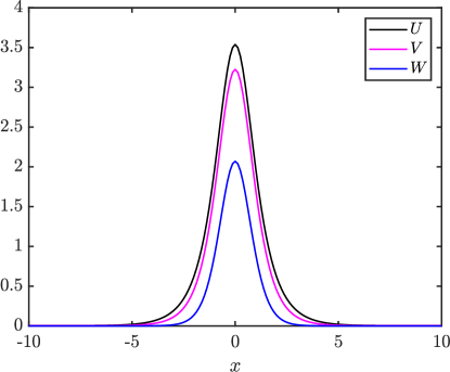
Figure 1: Profiles $U(x)$, $V(x)$, and $W(x)$ of a stable axisymmetric soliton in cross section $y=0$, obtained as a numerical solution of Eq. (11) with $k_{1}=0.6444,k_{2}=1.0763$, $b=0,q=+1$. The total power of this soliton, defined as per Eq. (2), is $P=100$.

Families of stable soliton solutions are characterized by the dependence of the total power, $P$, on the propagation constants, $k_{1,2}$, which is displayed in Fig. 2, for fixed values of the mismatch: (a) $q=0$; (b) $q=+1$; (c) $q=-1$. In each panel, colors represent different values of the birefringence: blue for $b=0$, red for $b=+0.5$, and green for $b=-0.5$.

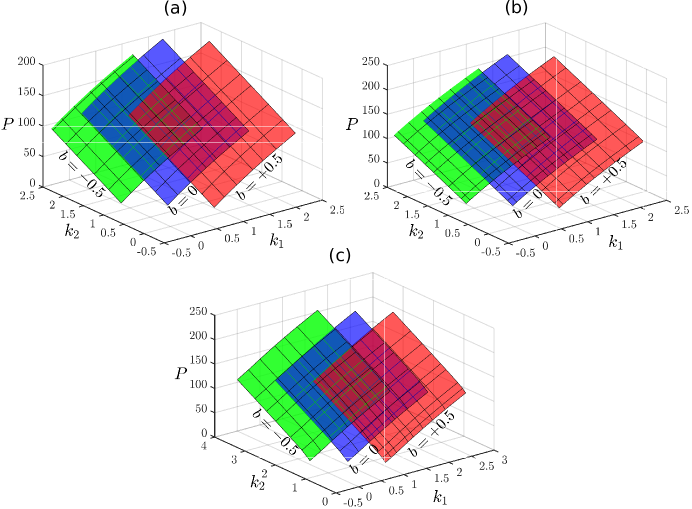
Figure 2: The total power (2) of solitons, $P(k_{1},k_{2})$, produced by the numerical solution of Eqs. (11), for different values of birefringence $b$, as indicated in the panels, and different values of the mismatch: (a) $q=0$, (b) $q=+1$, and (c) $q=-1$.

Two-dimensional solitons of the three-wave system with embedded vorticity are available too, but they all were found to be unstable against spontaneous splitting into fundamental (zero-vorticity) modes. The latter result, which may be construed as the modulational instability of a vortex ring against transverse perturbations, is not reproduced here, as it was demonstrated for $\chi^{(2)}$ systems previously Torner ; Mihalache .

Because the underlying equations (1) maintain the Galilean invariance, tilted solitons can be obtained from the straight ones by the application of the Galilean boost with components $\left(c,d\right)$:

$$u(x,y,z) = u_{\mathrm{sol}}(x-x_{0}-cz,y-y_{0}-dy)\exp\left[i\left(cx+dy\right)-\frac{i}{2}\left(c^{2}+d^{2}\right)z\right],~{}$$

$$v(x,y,z) = v_{\mathrm{sol}}(x-x_{0}-cz,y-y_{0}-dy)\exp\left[i\left(cx+dy\right)-\frac{i}{2}\left(c^{2}+d^{2}\right)z\right],~{}$$ (13)

$$w(x,y,z) = w_{\mathrm{sol}}(x-x_{0}-cz,y-y_{0}-dy)\exp\left[2i\left(cx+dy\right)-i\left(c^{2}+d^{2}\right)z\right].$$

In these expressions, $\left(x_{0},y_{0}\right)$ is the position of the soliton’s center at $z=0$.

It is relevant to attempt constructing a rotating bound state of two identical solitons, or three ones in the form of a rotating equilateral triangle, assuming that attraction between in-phase solitons attraction is in balance with the centrifugal force. This can be done looking for stationary two- and three-soliton solutions in the reference frame rotating with angular velocity $\omega$. The result is that such states with $\omega$ small enough can be produced, but they all are unstable. These results are illustrated by Figs. 3 and 4, respectively. The two- and three-soliton rotating bound states with parameters corresponding to Figs. 3 and 4 are found with the equilibrium distance between solitons being, respectively,

$$\left(l_{\mathrm{eq}}\right)_{\mathrm{2-sol}}\approx 5.926;~{}\left(l_{\mathrm{eq}}\right)_{\mathrm{3-sol}}\approx 11.936,$$ (14)

as shown in panels (a) of the figures. If the perturbation makes the distance slightly smaller than $l_{\mathrm{eq}}$, the solitons merge into a single one, while the perturbation which makes the distance slightly larger than $l_{\mathrm{eq}}$ splits the bound state into sets of gradually separating solitons, as seen in panels (b) and (c), respectively, of Figs. 3 and 4.

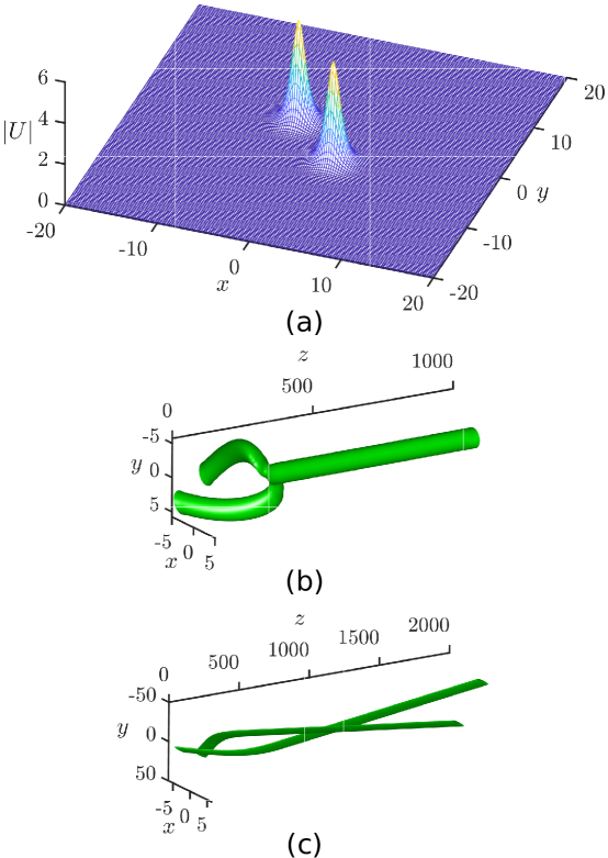
Figure 3: (a) The two-soliton stationary bound state, numerically found in the reference frame rotating with angular velocity $\omega=0.01$. This solution corresponds to propagation constants $k_{1}=0.7304$, $k_{2}=1.2773$ of the two FF components, while the total power is $P=227.14$. The mismatch and birefringence parameters are $q=+1$ and $b=0$. Panels (b) and (c) demonstrate instability of the two-soliton bound state by means of isosurfaces of $|u\left(x,y;z\right)|$, produced by direct simulations in the case when the distance between the two solitons is made, respectively, slightly smaller or larger than the equilibrium value given by Eq. (14).

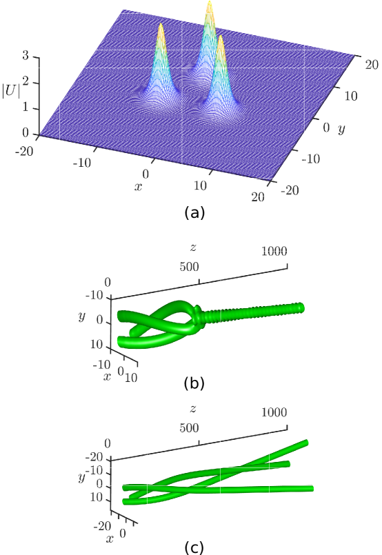
Figure 4: (a) The three-soliton stationary bound state, numerically found in the reference frame rotating with angular velocity $\omega=0.01$. This solution corresponds to propagation constants $k_{1}=0.40083$, $k_{2}=0.7139$ of the two FF components, while the total power is $P=211.12$. The mismatch and birefringence parameters are $q=+1$ and $b=0$. Panels (b) and (c) demonstrate instability of the three-soliton bound state by means of isosurfaces of $|u\left(x,y;z\right)|$, produced by direct simulations in the case when the distance between the two solitons is made, respectively, slightly smaller or larger than the equilibrium value given by Eq. (14).

III Collisional dynamics in the three-wave system

III.1 Soliton-soliton collisions

First, it is relevant to examine interactions between stable solitons in the three-component system. Here we focus on head-on collisions between identical solitons, generated by Eq. (13) under conditions

$$\left(x_{0}=y_{0}\right)_{1}=-\left(x_{0}=y_{0}\right)_{2}>0,\left(d=c\right)_{1}=-\left(d=c\right)_{2}>0,$$ (15)

where subscripts $1$ and $2$ pertain to the two solitons.

Systematic simulations of Eqs. (1) have demonstrated that slowly colliding solitons merge into a single quiescent one, while fast solitons collide quasi-elastically, separating with the original values of the tilt (with an “attempt” to create an additional quiescent soliton, which, however, decays). Typical examples of the merger and quasi-elastic collisions are displayed, severally, in Figs. 5(a) and (b).

The results are summarized in Fig. 6, which shows boundaries between the merger and quasi-elasticity regimes in the plane of $\left(P,c\right)$, assuming that the tilt parameters in Eq. (15) are taken as $c_{1,2}=d_{1,2}=\pm c$. The chart in Fig. 6 demonstrates essential dependence of the character of the collisions on the system’s mismatch, $q$, and weak dependence on the birefringence, $b$.

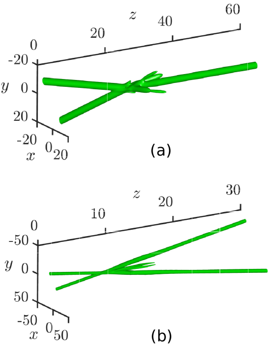
Figure 5: Isosurface plots of $\left|u\left(x,y;z\right)\right|$ illustrating head-on collisions of identical solitons solitons, with the total power $P=100$, as produced by simulations of Eq. (1) with $q=1,b=0.5$. The solitons are set in motion (in fact, tilted in the spatial domain) as per Eq. (15) with $c_{1,2}=\pm 0.5$ (a), and $c_{1,2}=\pm 1.5$ (b).

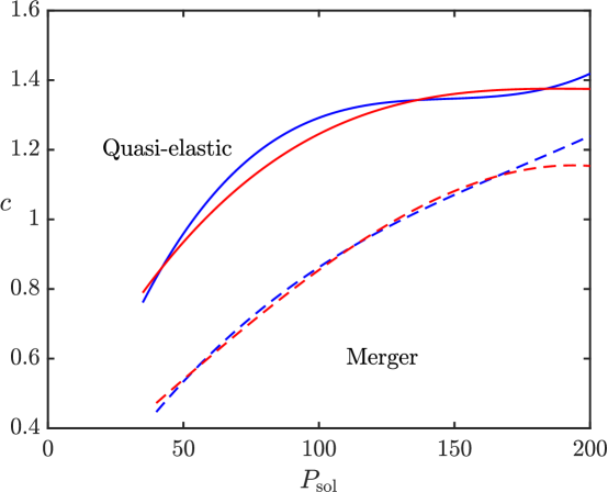
Figure 6: The border in the plane of the total power, $P_{\mathrm{sol}}$, and kick strength $c$ (see Eq. (15), between quasi-elastic collisions and collision-induced merger of the three-component solitons. The results are shown for two values of the mismatch, $q=+1$ and $-1$ (continuous and dashed lines, respectively), at two values of the birefringence coefficint, $b=0$ and and $0.5$ (blue and red lines, respectively).

III.2 Airy – Airy collisions

To simulate collisions between two TAWs carried by the $u$- and $v$-components of the FF field, initial conditions were taken as two mirror copies of the wave form (7), with equal amplitudes $u_{0}$ and opposite values of $\alpha$ and $\beta$. The waves are initially separated by distances $2x_{0}$ and $2y_{0}$ along the $x$ and $y$ axes (we set $x_{0}=y_{0}$):

$$u\left(x,y,z=0\right) = u_{0}\mathrm{Ai}\left(\alpha(x+x_{0})\right)\mathrm{Ai}\left(\beta(y+y_{0})\right)\exp\left(\aleph\alpha(x+x_{0})+\beth\beta(y+y_{0})\right),$$

$$v\left(x,y,z=0\right) = u_{0}\mathrm{Ai}\left(-\alpha(x-x_{0})\right)\mathrm{Ai}\left(-\beta(y-y_{0})\right)\exp\left(-\aleph\alpha(x-x_{0})-\beth\beta(y-y_{0})\right),$$ (16)

$$w\left(x,y,z=0\right) = 0,$$

cf. Eq. (9). While each wave form in isolation is an exact solution, the overlapping between them initiates nonlinear interaction through term $uv$ in the third equation of system (1). The opposite signs of $\alpha$ and $\beta$ imply that the two initial TAWs bend in opposite directions, as can be seen in Fig. 7 (the bend is small in the figure, as displaying it in a more pronounced form would require to run the simulations in a huge domain, while the size of the bend does not strongly affect the result of the collision).

A typical overall picture of the interaction in the space of $\left(x,y;z\right)$ and the corresponding final configuration are displayed, respectively, in Figs. 7 and 8. The outcome of the interaction is relatively simple: fusion of the colliding broad TAWs into a pair of well-separated narrow solitons with equal powers, accompanied by generation of conspicuous “debris”. It is relevant to mention that, in the 1D $\chi^{(2)}$ system, considered in work we3 , collision of TAWs also lead to creation of a set of solitons, but the number of emerging solitons was much larger – typically, between $7$ and $12$, with different powers of individual solitons. In fact, in the 1D setting the collision splits the colliding multi-peak Airy waves, each major peak giving rise to a soliton. On the contrary, in the 2D case the simulations actually reveal not splitting but fusion of the field into just two solitons. This observation is naturally explained by the stronger self-focusing effect in 2D. Indeed, in the cascading limit, which corresponds to large mismatch rev3 , the three-wave $\chi^{(2)}$ system may be reduced to a system of coupled nonlinear Schrödinger equations with the cubic self-focusing nonlinearity, which, by itself, leads to the 2D collapse Berge ; Sulem ; Fibich . Of course, the collapse is not eventually reached, as the cascading approximation eventually breaks down, but the trend to strong self-focusing is obvious in the 2D setting.

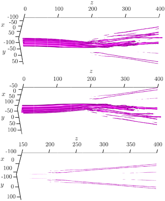
Figure 7: Isosurface plots of $\left|u\left(x,y;z\right)\right|$, $\left|v\left(x,y;z\right)\right|$, and $\left|w\left(x,y;z\right)\right|$ illustrating the collision of the TAWs, initiated by input (16) with $u_{0}=10$, $\alpha=\beta=-0.12$, $\aleph=\beth=0.125$, and separation distance $2x_{0}=2y_{0}=20$. The top, middle, and bottom panels represent the $u$-, $v$- and $w$-components, respectively. The collision leads to fusion of the three-component wave field into two separated narrow solitons, to which some “debris” is added. This outcome is additionally illustrated by Fig. 8.

Figure 8: Final amplitude profiles of the fields at $z=400$, corresponding to Fig. 7. The top, middle and bottom panels represent the $u$-, $v$- and $w$-components, respectively.

III.3 Collisions between Airy vortices

To consider the dynamics including TAW with imprinted vorticity (helicity), the simplest possibility is to add helical factors, $\exp\left(im_{u,v}\theta\right)$, with integer winding numbers $m_{u.v}$, to the input given by Eq. (16) ($\theta$ is the angular coordinate in the $\left(x,y\right)$ plane). Thus, the accordingly modified input is

$$u\left(x,y,z=0\right) = u_{0}\mathrm{Ai}\left(\alpha(x+x_{0})\right)\mathrm{Ai}\left(\beta(y+y_{0})\right)\exp\left(\aleph\alpha(x+x_{0})+\beth\beta(y+y_{0})\right)\exp\left(im_{u}\theta\right),$$

$$v\left(x,y,z=0\right) = u_{0}\mathrm{Ai}\left(-\alpha(x-x_{0})\right)\mathrm{Ai}\left(-\beta(y-y_{0})\right)\exp\left(-\aleph\alpha(x-x_{0})-\beth\beta(y-y_{0})\right)\exp\left(im_{v}\theta\right),$$ (17)

$$w\left(x,y,z=0\right) = 0.$$

Strictly speaking, this ansatz does not represent an exact TAW-vortex solution, but it corresponds to the experimentally relevant situation, in which vorticity is imparted to an available beam, such as TAW, by passing it through an appropriately designed helical phase plate plate ; plate2 or computer-generated hologram holo ; KH .

The nonlinear interaction between colliding helical TAWs is affected by the above-mentioned splitting instability of vortex solitons Torner ; Mihalache , which acts, as a transient effect, on the helical Airy modes as well. As a result, the collision converts the interacting vortical TAWs into a pair of well-separated narrow solitons, similar to what is demonstrated above in Figs. 7 and 8, to which additional solitons some “debris” are added. A typical example of the collision of the pair of mirror-symmetric TAWs with identical winding numbers, $m_{u}=m_{v}=1$, is displayed in Figs. 9 and 10.

Figure 9: The same as in Fig. 7, but for the collision of TAWs with superimposed vorticity, initiated by input (17) with equal winding numbers, $m_{u}=m_{v}=1$. The parameters are $u_{0}=10$, $\alpha=\beta=-0.12$, $\aleph=\beth=0.125$, and $2x_{0}=2y_{0}=20$.

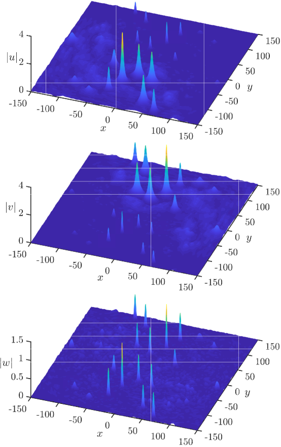
Figure 10: The final amplitude profiles at $z=500$ corresponding to Fig. 9. The top, middle and bottom panels display the $u$-, $v$- and $w$-components, respectively.

Further, a typical example of the collision between TAWs carrying opposite vorticities, i.e., $m_{u}=-m_{v}=1$, is presented by Figs. 11 and 12. In this case, the dominant dynamical factor is not the splitting instability of vortex rings, but the Kelvin-Helmholtz instability of counterpropagating azimuthal flows. Manifestations of this instability for optical vortices are known in nonlinear photonic media KH . It tends to produce a larger number of separated fragments. Accordingly, Figs. 11 and 12 demonstrate the creation of a pair of main narrow solitons, along with a cluster of small-amplitude fragments.

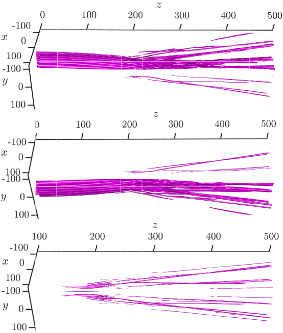
Figure 11: The same as in Fig. 9, but for the collision of Airy vortices with opposite vorticities, viz., $\left(m_{u},m_{v}\right)=(+1,-1)$ in Eq. (17). The parameters are $u_{0}=10$, $\alpha=\beta=0.12$, $\aleph=\beth=0.125$, and $x_{0}=y_{0}=50$.

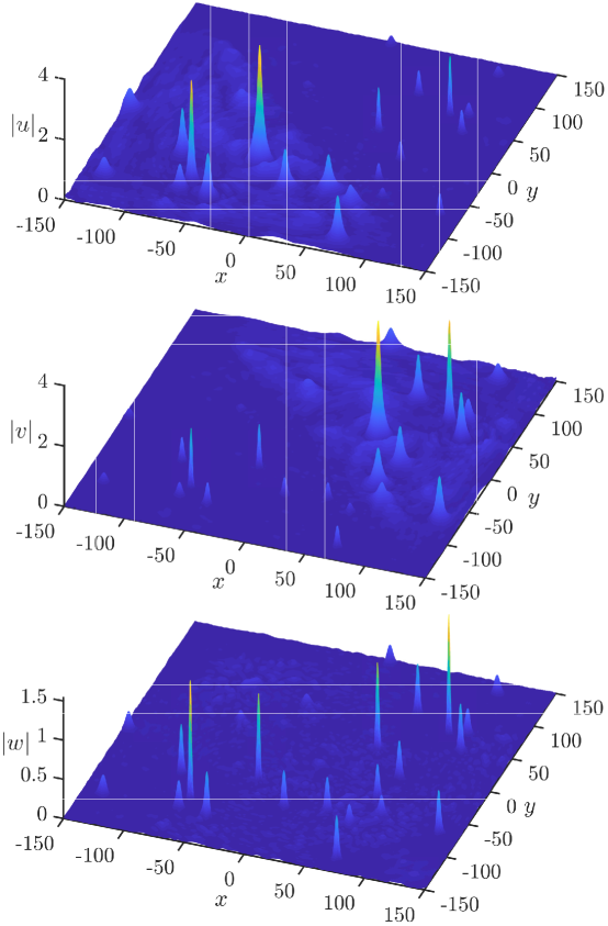
Figure 12: Final amplitude profiles at $z=400$ corresponding to Fig. 11. The top, middle and bottom panels display the $u$-, $v$- and $w$-components, respectively.

IV Airy – soliton collisions

Proceeding to collisions of solitons with TAWs, it is natural to consider the case when a relatively light soliton impinges upon a heavy Airy wave. Here, we present results for fixed parameters of the TAW,

$$\alpha=\beta=0.12,\aleph=\beth=0.125,$$ (18)

whose center is placed at $x_{0}=y_{0}=-50$, see the first line in Eq. (16). The amplitude of the incident soliton was taken to be equal to the TAW’s amplitude:

$$\left(\left|u_{\mathrm{sol}}\right|\right)_{\max}=u_{0}.$$ (19)

The soliton’s center was originally placed at $\left(x_{0}\right)_{\mathrm{sol}}=\left(y_{0}\right)_{\mathrm{sol}}=-70$, and tilt $c$ was applied to it as per Eq. (13). Data of the simulations were collected by varying $|c|$ from $0$ to $\approx 3.5$, and varying the soliton’s power between $P_{\mathrm{sol}}=50$ and $200$.

As shown in Fig. 13(a), relatively slow solitons, with $|c|\leq 1.4$, bounce back from the TAW. Note that rebound of the incident soliton was not observed in the 1D three-component system we3 , where a light soliton was always absorbed by the TAW. In the present system, the absorption takes place in an interval of $1.4\leq|c|\leq 2.6$, see Fig. 13(b). The soliton bouncing from the TAW or merging into it produces a visible perturbation, which, however, does not destroy the TAW. Finally, at $|c|\geq 2.6$, the fast soliton quickly passes the TAW, as seen in Fig. 13(c).

The results for the soliton-TAW collisions are summarized in Fig. 14, in the plane of $\left(P_{\mathrm{sol}},|c|\right)$. The general dependence of the critical value of the tilt constant, which is the boundary between the rebound and merger, on the power can be easily explained by the scaling relation between the tilt and total power, following from Eq. (1), if the birefringence and mismatch terms are neglected (i.e., the scaling is relevant for sufficient large values of the power): $c\sim\sqrt{P}$.

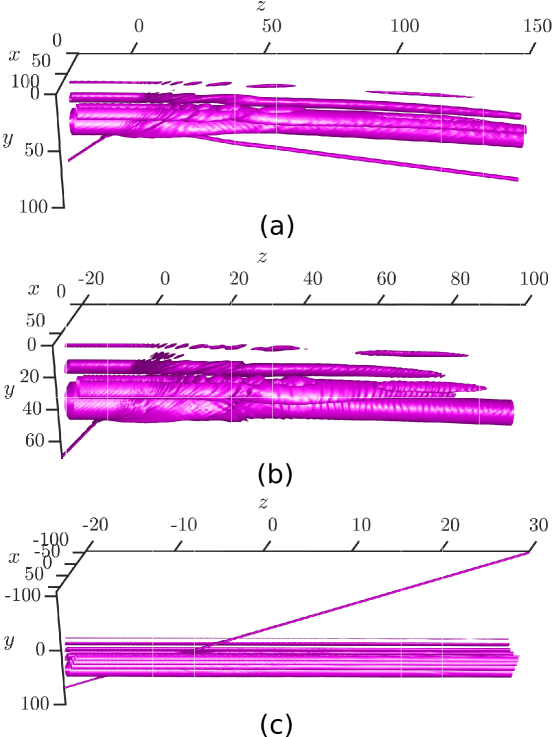
Figure 13: Isosurface plots of $\left|u\left(x,y;z\right)\right|$ illustrating collisions between the soliton with power $P_{\mathrm{sol}}=100$, corresponding to $k_{1}=1.1765$ and $k_{2}=0.5829$, and TAW with parameters fixed as per Eqs. (18) and (19), other constants being $q=1$ and $b=0.5$. The tilt is $c=-1.2$ in (a), $c=-2.0$ in (b), and $c=-3.5$ in (c). In panel (c) self-bending of the Airy wave is not visible, as the displayed interval of the propagation distance is too small for that.

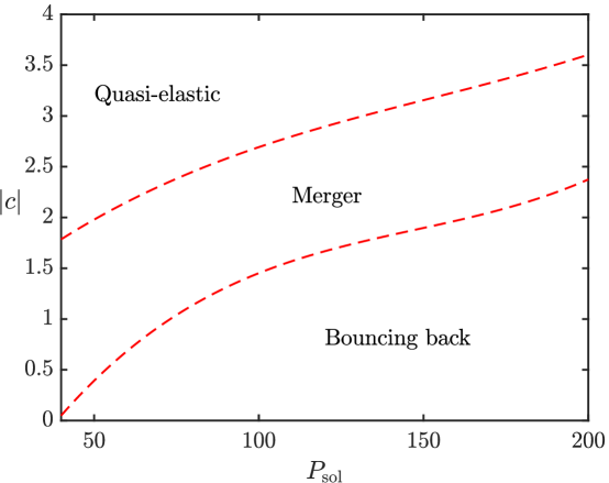
Figure 14: Borders in the plane of $\left(P_{\mathrm{sol}},|c|\right)$ separating different outcomes of the soliton-TAW collisions. TAW parameters are fixed as per Eqs. (18) and (19), other constants being $q=1$ and $b=0.5$.

Simulations of the collision of the incident soliton with the vortical TAW, generated as per input (17), produce results which are not essentially different from those displayed in Figs. 13 and 14.

V Conclusion

The present work aims to address specific dynamical effects demonstrated by TAWs (truncated Airy waves) and solitons in the 2D three-wave system of two FF (fundamental-frequency) and SH (second-harmonic) fields coupled by the $\chi^{(2)}$ terms in the optical medium. A unique peculiarity of the system is that TAW states, carried by a single FF component, which are represented by exact analytical solutions, are stable against small perturbations in the form of seeds of the other components. The same system give rise to stable three-component solitons, which can be found in the numerical form. These facts suggest possibilities to consider interactions between TAWs carried by the different FF components (they interact nonlinearly through the SH field), as well as collisions between solitons and TAWs. Previously, these possibilities were explored in the 1D system, while the present work addresses the 2D setting. In particular, the present system makes it possible to consider interactions involving TAWs onto which vorticity is imprinted.

First, the interaction of two TAWs, originally created as mirror images of each other in the different FF components, leads to the fusion of the fields into a pair of well-separated narrow solitons. The character of the interaction is opposite to that in the 1D three-wave system, where, instead of the fusion, the interaction leads to fission of the colliding TAWs into a large number of secondary solitons. The interaction of 2D TAWs with imprinted vorticity is affected by the transient splitting instability of vortex rings, in the case when both TAWs carry the identical vorticity. In this case, the interaction generates an additional pair of solitons. In the case of opposite vorticities of the interacting TAWs, there appears a cluster of fragments, produced by the transient Kelvin-Helmholtz instability of the counter-rotating vortices. Further, the systematic numerical study of collisions of relatively light solitons with a heavy TAW demonstrates that a slowly moving soliton bounces back, a faster one is absorbed by the TAW, while fast collision is quasi-elastic. As concerns soliton-soliton collisions, it is shown here that they lead to merger of slow solitons into a single one, or quasi-elastic passage of fast solitons.

A challenging possibility for the development of the analysis is to extend it to the three-dimensional system governing the spatiotemporal propagation of waves in $\chi^{(2)}$ media, where solitons may be stable too Rub ; HH . In particular, one may expect that the interaction of 3D Airy waves may be more violent because the cubic nonlinear Schrödinger equations, to which the $\chi^{(2)}$ system reduces in the cascading limit gives rise to the supercritical collapse Berge ; Sulem ; Fibich .

References

- (1) Berry M V and Balazs N L 1979 Non-spreading wave packets Am. J. Phys. 47 264-267
- (2) G. A. Siviloglou and D. N. Christodoulides 2007 Accelerating finite energy Airy beams Opt. Lett. 32, 979
- (3) G. A. Siviloglou, J. Broky, A. Dogariu, and D. N. Christodoulides 2007 Observation of Accelerating Airy Beams Phys. Rev. Lett. 99, 213901
- (4) P. Polynkin, M. Kolesik, J. V. Moloney, G. A. Siviloglou, and D. N. Christodoulides 2009 Curved plasma channel generation using ultraintense Airy beams Science 324, 229-232
- (5) P. Rose, F. Diebel, M. Boguslawski, and C. Denz 2013 Airy beam induced optical routing Appl. Phys. Lett. 102, 101101
- (6) R. Driben, Y. Hu, Z. Chen, B. A. Malomed, and R. Morandotti 2013 Inversion and tight focusing of Airy pulses under the action of third-order dispersion Opt. Lett. 38, 2499-2501
- (7) C. Hang and G. Huang 2014 Guiding ultraslow weak-light bullets with Airy beams in a coherent atomic system Phys. Rev. A 89, 013821
- (8) N. K. Efremidis 2014 Accelerating beam propagation in refractive-index potentials”, Phys. Rev. A 98, 023841
- (9) N. K. Efremidis, V. Paltoglou, and W. von Klitzig 2013 Accelerating and abruptly autofocusing matter waves Phys. Rev. A 87, 043637
- (10) Rozenman G G, Fu S H, Arie A, Shemer L 2019 Quantum mechanical and optical analogies in surface gravity water waves Fluids 4 96
- (11) A. Minovich, A. E. Klein, N. Janunts, T. Pertsch, D. N. Neshev, and Y. S. Kivshar 2011 Generation and near-field imaging of Airy surface plasmons Phys. Rev. Lett. 107, 116802
- (12) L. Li, T. Li, S. M. Wang, C. Zhang, and S. N. Zhu 2011 Plasmonic Airy Beam Generated by In-Plane Diffraction Phys. Rev. Lett. 107, 126804
- (13) I. Epstein and A. Arie 2014 Arbitrary Bending Plasmonic Light Waves Phys. Rev. Lett. 112, 023903
- (14) M. Clerici, Y. Hu, P. Lassonde, C. Milián, A. Couairon, D. N. Christodoulides, Z. Chen, L. Razzari, F. Vidal, F. Légaré, D. Faccio, R. Morandotti 2015 Laser-assisted guiding of electric discharges around objects Sci. Adv. 1, e140011
- (15) J. Baumgartl, M. Mazilu, and K. Dholakia 2008 Optically mediated particle clearing using Airy wavepackets Nature Photonics 2, 675-678
- (16) N. Voloch-Bloch, Y. Lereah, Y. Lilach, A. Gover, and A. Arie 2013 Generation of electron Airy beams Nature 494, 331-335
- (17) I. Kaminer, M. Segev, and D. N. Christodoulides 2011 Self-accelerating self-trapped optical beams Phys. Rev. Lett. 106, 213903
- (18) Y. Fattal, A. Rudnick, and D. M. Marom 2011 Soliton shedding from Airy pulses in Kerr media Opt. Exp. 19, 17298-17307
- (19) A. Rudnick and D. M. Marom 2011 Airy-soliton interactions in Kerr media Opt. Exp. 19, 25570-25582.
- (20) Y. Hu, Z. Sun, D. Bongiovanni, D. Song, C. Lou, J. Xu, Z. Chen, and R. Morandotti 2012 Reshaping the trajectory and spectrum of nonlinear Airy beams Opt. Lett. 37, 3201-3203
- (21) Y. Zhang, M. Belić, Z. Wu, H. Zheng, K. Lu, Y. Li, and Y. Zhang 2013 Soliton pair generation in the interactions of Airy and nonlinear accelerating beams Opt. Lett. 38, 4585-4588
- (22) I. M. Allayarov and E. N. Tsoy 2014 Dynamics of Airy beams in nonlinear media Phys. Rev. A 90, 023852
- (23) C. Ruiz-Jiménez, K. Z. Nóbrega, and M. A. Porras 2015 On the dynamics of Airy beams in nonlinear media with nonlinear losses Opt. Exp. 23, 8918-8928
- (24) M. Shen, W. Li, and R.-K. Lee 2016 Control on the anomalous interactions of Airy beams in nematic liquid crystals Opt. Exp. 24, 8501
- (25) L. Zhang, P. Huang, C. Conti, Z. Wang, Y. Hu, D. Lei, Y. Li, and D. Fan 2017 Decelerating Airy pulse propagation in highly non-instantaneous cubic media Opt. Exp.. 25, 1856-1866
- (26) T. Ellenbogen, N. Voloch-Bloch, A. Ganany-Padowicz, and A. Arie 2009 Nonlinear generation and manipulation of Airy beams Nature Phot. 3, 395-398
- (27) I. Dolev, T. Ellenbogen, and A. Arie 2010 Switching the acceleration direction of Airy beams by a nonlinear optical process Opt. Lett. 35, 1581-1583
- (28) I. Dolev, I. Kaminer, A. Shapira, M. Segev, and A. Arie 2012 Experimental Observation of Self-Accelerating Beams in Quadratic Nonlinear Media Phys. Rev. Lett. 108, 113803
- (29) T. Mayteevarunyoo and B. A. Malomed 2015 Generation of solitons from the Airy wave through the parametric instability Opt. Lett. 40, 4947-4950
- (30) T. Mayteevarunyoo and B. A. Malomed 2016 Two-dimensional solitons generated by the downconversion of Airy waves Opt. Lett. 41, 2919-2922
- (31) Mayteevarunyoo T and Malomed B A 2017 The interaction of Airy waves and solitons in the three-wave system J. Optics 19 085501
- (32) G. I. Stegeman, D. J. Hagan, and L. Torner 1996 Cascading phenomena and their applications to all-optical signal processing, mode-locking, pulse compression and solitons Opt. Quant. Elect. 28, 1691-1740
- (33) C. Etrich, F. Lederer, B. A. Malomed, T. Peschel, and U. Peschel 2000 Optical solitons in media with a quadratic nonlinearity Prog. Opt. 41, 483-568
- (34) A. V. Buryak, P. Di Trapani, D. V. Skryabin, and S. Trillo 2002 Optical solitons due to quadratic nonlinearities: from basic physics to futuristic applications Phys. Rep. 370, 63-235
- (35) Dai H T, Liu Y J, Luo D and Sun X W 2010, Propagation dynamics of an optical vortex imposed on an Airy beam Opt Lett 35 4075-4077
- (36) Khonina S N 2011 Specular and vortical Airy beams Opt. Commun. 284 4263-4271
- (37) Jiang Y F, Huang K K and Lu X H 2012 Propagation dynamics of abruptly autofocusing Airy beams with optical vortices Opt. Exp. 20 18579-18584
- (38) Li P, Liu S, Peng T, Xie, G F, Gan X T, Zhao, J L 2014 Spiral autofocusing Airy beams carrying power-exponent-phase vortices Opt. Exp. 22 7598-7606
- (39) Chen B, Chen, C D, Peng X, Peng, Y L, Zhou M L, Deng D M 2015 Propagation of sharply autofocused ring Airy Gaussian vortex beams Opt. Exp. 23 19288-19298
- (40) Drummond P D, Kheruntsyan K V and He H 1998 Coherent molecular solitons in Bose-Einstein condensates Phys. Rev. Lett. 81 3055-3058
- (41) Yang J K and Lakoba T I 2007 Universally-convergent squared-operator iteration methods for solitary waves in general nonlinear wave equations Stud. Appl. Math. 118 153-197
- (42) Yang J K 2008 Iteration methods for stability spectra of solitary waves J. Comp. Phys. 227 6862-6876
- (43) Malomed B A 1998 Potential of interaction between two- and three-dimensional solitons Phys. Rev. E 58 7928-7933
- (44) Torres P, Soto-Crespo J M, Torner L, and Petrov D V 1998 Solitary-wave vortices in type II second-harmonic generation Opt. Commun. 149, 77-83
- (45) He S, Malomed B A, Mihalache D, Peng X, Yu X, He Y, and Deng D 2021 Propagation dynamics of abruptly autofocusing circular Airy Gaussian vortex beams in the fractional Schrödinger equation Chaos, Solitons & Fractals 142 110470
- (46) He S, Malomed B A, Mihalache D, Peng X, He Y, and Deng D 2021 Propagation dynamics of radially polarized symmetric Airy beams in the fractional Schrödinger equation Phys. Lett. A 404 127403
- (47) Mihalache D, Mazilu D, Crasovan L-C, Towers I, Malomed B A, Buryak A V, Torner L, and Lederer F 2002 Stable three-dimensional spinning optical solitons supported by competing quadratic and cubic nonlinearities Phys. Rev. E 66 016613
- (48) Bergé L 1998 Wave collapse in physics: principles and applications to light and plasma waves Phys. Rep. 303, 259-370
- (49) Sulem C and Sulem P-L The Nonlinear Schrödinger Equation: Self-Focusing and Wave Collapse (Springer, New York, 1999)
- (50) Fibich G The Nonlinear Schrödinger Equation: Singular Solutions and Optical Collapse (Springer, Heidelberg, 2015)
- (51) Kotlyar V V, Almazov A A, Khonina S N, Soifer V A, Elfstrom H and Turunen 2005 Generation of phase singularity through diffracting a plane or Gaussian beam by a spiral phase plate J. Opt. Soc. Am. A 22 849-861
- (52) Wang X W, Nie Z Q, Liang Y, Wang J, Li T and Jia B H 2018 Recent advances on optical vortex generation Nanophotonics 7 1533-1556
- (53) Rozas D, Law C T and Swartzlander G A Propagation dynamics of optical vortices 1997 J. Opt. Soc. Am. B 14 3054-3065
- (54) Carpentier A V, Michinel H Salgueiro J 2008 Making optical vortices with computer-generated holograms Am. J. Phys. 76 916-921
- (55) Kanashov A A and Rubenchik A M 1981 On diffraction and dispersion effect on three wave interaction Physica D 4 122-134
- (56) Malomed B A, Drummond P, He H, Berntson A, Anderson D and Lisak M 1997 Spatio-temporal solitons in optical media with a quadratic nonlinearity Phys. Rev. E 56 4725-4735