Data-driven and constrained optimization of semi-local exchange and non-local correlation functionals for materials and surface chemistry

Abstract

Reliable predictions of surface chemical reaction energetics require an accurate description of both chemisorption and physisorption. Here, we present an empirical approach to simultaneously optimize semi-local exchange and non-local correlation of a density functional approximation to improve these energetics. A combination of reference data for solid bulk, surface, and gas-phase chemistry and physical exchange-correlation model constraints leads to the VCML-rVV10 exchange-correlation functional. Owing to the variety of training data, the applicability of VCML-rVV10 extends beyond surface chemistry simulations. It provides optimized gas phase reaction energetics and an accurate description of bulk lattice constants and elastic properties.

VCML-rVV10 is a meta-GGA exchange-correlation functional which has been derived from a simultaneous optimization of semi-local exchange and non-local, i.e., van der Waals correlation. Training the functional on a variety of physical and chemical data as well as enforcing a number of constraints of the exact functional makes VCML-rVV10 accurate for surface chemistry without compromising on the prediction of bulk lattice constants and molecular interactions.

I Introduction

Kohn-Sham (KS) density functional theory (DFT)^{1, 2} is one of the most widely used electronic structure theories. It provides reasonable accuracy for many physical properties of atoms, molecules, surfaces, and solids.³ For the practical use of KS DFT, approximations to electronic exchange and correlation (XC) are needed. These so-called XC functionals have been developed for decades.^{4, 5} There is a variety of both empirical^{6, 7, 8, 9} and non-empirical functionals.^{10, 11, 12, 13, 14} In the latter approaches it was established that fulfilling analytical constraints¹⁵ leads to functionals with improved predictions of molecular and bulk properties.^{12, 16, 17} Typically, empirical as well as non-empirical functionals describe some physical and chemical properties with improved accuracy at the price of worse predictions of other properties.

To obtain an XC functional that accurately describes a wide range of physical properties, strategies from the empirical and non-empirical XC functional development approaches can be combined. Constraints from the latter can be imposed while fitting a multi-parameter empirical XC functional form to experimental and quantum chemistry reference data.

There are several approaches combining constraints and data for XC functionals.^{18, 19, 20} Recently, our group has applied such a combined approach to construct a multi-purpose, constrained and machine learned (MCML) XC functional. MCML shows improved predictions of surface and gas phase reactions without sacrificing the good description of bulk properties.¹⁸ The MCML functional is a so-called semi-local functional, lacking an explicit description of non-local, i.e., van der Waals (vdW) type correlation. Supplementing a semi-local functional with vdW correlation does not only affect the performance for vdW-dominated interactions. For example, some semi-local approximations tend to overbind chemisorbed systems.^{21, 22} Adding attractive dispersion forces can increase this tendency even further. The semi-local part of a functional can be optimized to compensate for effects of overbinding or lattice spacing contraction from the attractive vdW terms.^{23, 24} On the other hand, the vdW part can be optimized using, e.g., the parameterized, semi-empirical rVV10 non-local vdW term.^{25, 26, 27} With that, performance on dispersion-dominated benchmark data is optimized while fixing the underlying semi-local functional.

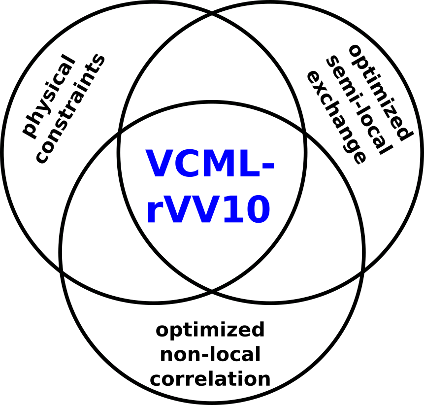
Figure 1: Basic outline of the VCML-rVV10 optimization.

In the present work, we optimize the semi-local exchange and non-local correlation parts of a vdW XC functional simultaneously for several bulk, surface, and gas phase property predictions. This simultaneous optimization of the semi-local exchange functional form and an rVV10 non-local term enables us to construct a functional that is accurate for a range of materials properties governed by different types of chemical bonds. There is no compromise between the accuracy for the description of ionic, covalent or metallic bonds and dispersive interactions, or vice versa. Incorporating physical constraints into this empirical approach leads to the VCML-rVV10 functional (vdW functional using constraints and machine learning, employing the rVV10 formalism), see Fig. 1. This name shall clearly separate our functional from MCML. The semi-local exchange functional parts of MCML and VCML(-rVV10) are different, and the latter is not simply a vdW-supplemented form of MCML. While we optimize the semi-local exchange as well as the non-local correlation part of our functional, for semi-local correlation we employ REGTPSS,²⁸ in analogy to Brown et al.¹⁸

This article is structured as follows. In Section II, a brief introduction of the theoretical background including the rVV10 formalism is given. The used computational parameters are shown in Section III. All employed data sets are described in Section IV. Thereafter, our functional optimization approach is presented in Section V. The main results are discussed in Section VI. A conclusion is presented in Section VII.

II Theoretical background

Atomic units are being used throughout this section. In the KS formulation of DFT, the total energy of a system with total electron density

$$n(\textbf{r})=n^{\uparrow}(\textbf{r})+n^{\downarrow}(\textbf{r}),$$ (1)

where $n^{\uparrow}$ and $n^{\downarrow}$ are the spin densities of a system with collinear spins, can be expressed as

$$E^{\text{KS}}=T_{\text{S}}[n^{\uparrow},n^{\downarrow}]+E_{\text{ext}}[n]+E_{\text{H}}[n]+E_{\text{XC}}[n^{\uparrow},n^{\downarrow}].$$ (2)

Here, $T_{\text{S}}$ is the non-interacting kinetic energy, $E_{\text{ext}}$ is the energy of the interaction with an external potential, and $E_{\text{H}}$ is the Hartree energy of the electrons. Exchange and correlation effects are treated via the exchange-correlation functional $E_{\text{XC}}$.

The electron density is the fundamental building block of DFT. It determines the energy as well as any other property. While DFT is in principle exact, the $E_{\text{XC}}$ needs to be approximated. Such approximations can be categorized according to their ingredients in the functional form. This is known as the Jacob’s ladder of DFT.²⁹ The lowest rung is given by the local (spin) density approximation (LSDA). Only the density itself is taken as a parameter. Additionally including the density gradient characterizes generalized gradient approximations (GGAs). Meta-GGAs also include a dependence on the kinetic energy density of the occupied orbitals.

The exchange energy for meta-GGAs is defined as an integral of the exchange energy density per electron of the homogeneous electron gas (HEG) at density $n(\textbf{r})$

$$\epsilon^{\rm HEG}_{\text{X}}[n(\textbf{r})]=-\frac{3}{4}(3/\pi)^{1/3}n(\textbf{r})^{1/3},$$ (3)

multiplied by an exchange enhancement factor $F_{\text{X}}$

$$E_{\text{X}}[n(\textbf{r})]=\int\text{d}^{3}rn(\textbf{r})\epsilon^{\text{HEG}}_{\text{X}}[n(\textbf{r})]F_{\text{X}}(s(\textbf{r}),\alpha(\textbf{r})).$$ (4)

Here,

$$s(\textbf{r})=\frac{|\bm{\nabla}n(\textbf{r})|}{2k_{\text{F}}(\textbf{r})n(\textbf{r})}$$ (5)

is the reduced density gradient with the Fermi wave vector

$$k_{\text{F}}(\textbf{r})=\sqrt[3]{3\pi^{2}n(\textbf{r})}.$$ (6)

The dependence on the kinetic energy density can be described as

$$\alpha(\textbf{r})=\frac{\tau^{\text{KS}}(\textbf{r})-\tau^{\text{Weizs\"{a}cker}}(\textbf{r})}{\tau^{\text{HEG}}(\textbf{r})},$$ (7)

with

$$\tau^{\text{KS}}(\textbf{r}) =\frac{1}{2}\sum_{i}f_{i}|\bm{\nabla}\phi_{i}(\textbf{r})|^{2},$$ (8)

$$\tau^{\text{Weizs\"{a}cker}}(\textbf{r}) =|\bm{\nabla}n(\textbf{r})|^{2}/(8n(\textbf{r})),$$ (9)

$$\tau^{\text{HEG}}(\textbf{r}) =\frac{3}{10}(3\pi^{2})^{2/3}n(\textbf{r})^{5/3}$$ (10)

being the kinetic energy density based on the KS orbitals $\phi_{i}(\textbf{r})$ with occupation $f_{i}$, the von Weizsäcker kinetic energy density describing the single orbital limit, and the non-interacting kinetic energy density of a HEG at density $n(\textbf{r})$, respectively. The term $\tau^{\text{Weizs\"{a}cker}}(\textbf{r})$ vanishes for zero charge density gradient and equals $\tau^{\text{KS}}(\textbf{r})$ for a single orbital density. Accordingly, Eq. (7) approaches zero in the single orbital limit and one in the homogeneous limit where $\bm{\nabla}n(\textbf{r})=0$ and $\tau^{\text{KS}}(\textbf{r})=\tau^{\text{HEG}}(\textbf{r})$. With that, the parameter $\alpha$ can characterize the type of bonding in a system.

For spin-polarized systems, $E_{\text{X}}$ is obtained via the spin scaling relation

$$E_{\text{X}}[n^{\uparrow}(\textbf{r}),n^{\downarrow}(\textbf{r})]=\frac{E_{\text{X}}[2n^{\uparrow}(\textbf{r})]+E_{\text{X}}[2n^{\downarrow}(\textbf{r})]}{2}.$$ (11)

The exchange-enhancement factor $F_{\text{X}}$ is optimized in this work by training against reference data, see Section V for more details.

In the rVV10^{25, 26} methodology, a non-local correlation energy is introduced as

$$E_{\text{c,nl}}=\frac{1}{2}\int\int\text{d}^{3}r\text{d}^{3}r^{\prime}n(\textbf{r})\Theta(n(\textbf{r}),n(\textbf{r}^{\prime}))n(\textbf{r}^{\prime}).$$ (12)

The non-local kernel as described by Sabatini et al. ²⁶ is given by

$$\Theta(n(\textbf{r}),n(\textbf{r}^{\prime}))^{\text{rVV10}}=-\frac{3}{2}\frac{1}{(q(\textbf{r})R^{2}+1)(q^{\prime}(\textbf{r}^{\prime})R^{2}+1)(q(\textbf{r})R^{2}+q^{\prime}(\textbf{r}^{\prime})R^{2}+2)},$$ (13)

in which

$$q(\textbf{r})=\frac{\omega_{0}(n(\textbf{r}),|\bm{\nabla}n(\textbf{r})|)}{k(\textbf{r})}$$ (14)

and $R=|\textbf{r}-\textbf{r}^{\prime}|$. The same expression is obtained for $q^{\prime}$ by replacing r with $\textbf{r}^{\prime}$. The term $\omega_{0}$ depends on the local band gap as well as the plasma frequency. For more information, see Sabatini et al. ²⁶ as well as the supporting information (SI), Sec. 1. Importantly for further discussion, the term

$$k(\textbf{r})=3\pi b\left(\frac{n(\textbf{r})}{9\pi}\right)^{\frac{1}{6}}$$ (15)

determines the short-range damping of the $R^{-6}$ divergence of the non-local kernel. The parameter $b$ needs to be optimized for any functional $E_{\text{XC}}$ that $E_{\text{c,nl}}$ is added to. Simply speaking, the larger the $b$ parameter, the weaker the vdW interaction. The optimization of this parameter is discussed in Section V. For additional details we refer to the original works of Vydrov and Van Voorhis ²⁵ and Sabatini et al.²⁶

III Computational details

In this work, the Vienna ab initio Simulation Package (VASP)³⁰ was employed. The DFT calculations were carried out using projector-augmented wave³¹ pseudopotentials³² which are based on PBE¹⁰ all-electron atomic calculations, and a plane wave basis set. An energy cutoff of 1000 eV (73.50 Ry or 36.75 $E_{\text{h}}$) was used together with an electronic SCF tolerance of 10^-7 eV. For geometry optimizations, forces were converged such that the maximum force per atom is at most 10^-2 eV/Å. Note that in the ADS41 set (see SI, Tab. ST25), {H₂O,CH₃OH}@Pt111 using SCAN¹² and {H₂O,CH₃OH,C₃H₈,C₄H₁₀}@Pt111 using SCAN-rVV10²⁷ required a looser criterion of $2\cdot 10^{-2}$ eV/Å  because of numerical instabilities, which are absent in r²SCAN.¹⁴ The k-point spacing for the surface (in 2 dimensions) and bulk (in 3 dimensions) calculations was at most 0.018 Å^-1. A Gaussian smearing of KS occupation numbers with a width of $2\cdot 10^{-2}$ eV was used for surfaces and bulk systems.

For data sets involving molecules, the unit cell has been prepared as follows. Around the largest system in the set, a box was constructed such that there is at least 20 Å in between periodic images in all directions. This box was employed for all molecules in the corresponding data set. For atoms, a cell of 23 Å was used.

To compare the performance of the VCML-rVV10 functional, calculations were also performed with PBE,¹⁰ PBE-D3,^{10, 33} MS2,³⁴ SCAN,¹² r²SCAN,¹⁴ SCAN-rVV10,²⁷ MCML,¹⁸ and MCML-rVV10 (introduced in this work). For the error analysis, the mean error (ME) and mean absolute error (MAE) are computed

ME $$=\frac{1}{N}\sum_{i=1}^{N}x_{i}^{\text{calc}}-x_{i}^{\text{ref}}$$ (16)

MAE $$=\frac{1}{N}\sum_{i=1}^{N}\left|x_{i}^{\text{calc}}-x_{i}^{\text{ref}}\right|,$$ (17)

where $x_{i}^{\text{calc}}$ is the calculated value and $x_{i}^{\text{ref}}$ the corresponding reference value. These values are provided in the SI, Tab. ST7, 9, 11-20, 22-25 and 27. All individual errors for any system of a data set are computed by $x_{i}^{\text{calc}}-x_{i}^{\text{ref}}$.

IV Benchmark data sets

To obtain a multi-purpose XC functional from the proposed methodology, see Section V, a variety of training data is required. Our training data consists of molecular, surface as well as bulk properties, as described below. The systems of each data set and all calculated properties are provided in the SI, Tab. ST6-27.

The DBH24 set³⁵

consists of 12 forward and 12 reverse reaction barrier heights of small molecules. Reference values are the best estimates, consisting of quantum chemical and experimental data, according to Zheng et al.³⁶ Total energies were computed on the reference structures; no structural optimizations were carried out.

The RE42 set²³

contains 42 reaction energies involving 45 molecules of the G2/97³⁷ test set. Experimental reference values are taken from Wellendorff et al.²³ The geometries of all molecules were fully optimized before their total energy was used to calculate the reaction energies.

The S66x8 set³⁸

has 66 molecular complexes at eight distances, the interaction of which is dominated by non-covalent bonding. Reference values are the recommended dissociation energies, calculated by MP2-F12 energies at the basis set limit combined with CCSD(Tc${}_{\text{sc}}$)-F12 correlation, according to Brauer et al.³⁹ Total energies were computed at the reference geometries, thus no geometry optimizations were carried out.

The W4-11 set⁴⁰

contains 140 atomization energies of small to medium sized molecules. Reference values are taken from Karton et al.,⁴⁰ which are based on the Weizmann-4 (W4) computational thermochemistry method. No structural optimizations were carried out, and total energies were computed on the reference structures.

The SOL62 set

is based on a set of 64 solids proposed by Zhang et al.¹⁷ Of that set we removed all elements heavier than Au, as for those systems (Pb, Th) the predicted errors will typically be very large due to strong relativistic effects.²³ The reference values are taken from the supplemental information of Zhang et al.,¹⁷ where zero-point energy corrections of PBE were subtracted from the experimental values. All unit cells were fully optimized. Afterwards, the lattice constants $a_{\text{lat}}$ and bulk moduli $B$ were computed using an equation of state (EOS) fit⁴¹ from five energies around and at the minimum volume. Further, cohesive energies $E_{\text{coh}}$ were computed with respect to the isolated atoms in their energetically preferred magnetic ground state. This data set is split into the three subset $a_{\text{lat}}$@SOL62, $E_{\text{coh}}$@SOL62, and $B$@SOL62.

The ADS41 set^{42, 22}

consists of 41 surface reaction energies. Experimental reference values are taken from the collection in Sharada et al.²² The atomic positions of the isolated molecules, the isolated surfaces as well as the combined systems were optimized. For the clean surfaces and the combined systems, the cell was constrained to the bulk lattice dimensions, while introducing at least 15 Å of vacuum in the out-of-plane direction. The vacuum layer is the same for the isolated surface and the combined system, ensuring consistent results. The surfaces are constructed to have 4 layers. The lower two are fixed at the bulk lattice positions, while the top two layers (and the adsorbed molecule) are optimized. Adsorption energies are computed per adsorbate, thus the total adsorption energy is divided by the number of adsorbates in the computational cell. Because ADS41 contains Co and Ru surfaces, we additionally optimized the unit cells of either hcp solid to obtain the corresponding lattice constants. These solids are not part of the SOL62 set, and were only optimized for ADS41. The ADS41 data set is subdivided into physisorption-dominated reactions (15 reaction energies, denoted as $E_{\text{ads}}^{\text{phy}}$@ADS41) and chemisorption-dominated reactions (26 reaction energies, denoted as $E_{\text{ads}}^{\text{che}}$@ADS41).

V Functional fitting approach

V.1 General outline

In the following, the meta-GGA as well as the vdW fitting procedure is presented. The procedure to obtain the meta-GGA functional form has been outlined in Brown et al. ¹⁸ for the MCML functional. We will briefly discuss its main components here. Our exchange enhancement factor is expanded in a series of Legrendre polynomials $P$ for $s$ and $\alpha$ as

$$F_{\text{X}}(s(\textbf{r}),\alpha(\textbf{r}))=\sum_{i=0}^{7}\sum_{j=0}^{7}c_{ij}P_{i}\left(\hat{s}(\textbf{{r}})\right)P_{j}\left(\hat{\alpha}(\textbf{r})\right),$$ (18)

where

$$\hat{s}(\textbf{r})=\frac{2s(\textbf{r})^{2}}{\eta+s(\textbf{r})^{2}}-1$$ (19)

maps the semi-infinite interval of reduced density gradients $s$ to the interval spanned by the Legrendre polynomials, $[-1,1]$. Here, $\eta=\kappa/\mu^{\rm GE}$ is used to represent the exchange enhancement of PBEsol¹¹ by the first two Legendre polynomials $P_{0}\!\left(\hat{s}(\textbf{{r}})\right)$ and $P_{1}\!\left(\hat{s}(\textbf{{r}})\right)$. Further, $1+\kappa=1.804$ is the local Lieb-Oxford bound,^{43, 44} and $\mu^{\rm GE}=10/81$ is the lowest-order coefficient of the gradient correction to the free electron gas exchange energy.⁴⁵ Similarly,

$$\hat{\alpha}(\textbf{r})=\frac{(1-\alpha(\textbf{r})^{2})^{3}}{1+\alpha(\textbf{r})^{3}+4\alpha(\textbf{r})^{6}}$$ (20)

maps the semi-infinite interval of $\alpha$ to the interval $[-0.25,1]$. This form of $\hat{\alpha}$ coincides with the GGA-weighting function of the MS2 functional.³⁴ The transformations of $s$ and $\alpha$ are visualized in the SI, Fig. SF1. Optimizing the 64 coefficients $c_{ij}$ in Eq. (18), as described in the next sections, delivers an optimal semi-local meta-GGA functional. The physical constraints introduced for MCML are also applied to our functional, i.e., the LDA limit with $F_{\text{X}}=1$ for $s=0$ and $\alpha=1$, the exchange gradient expansion for $s\approx 0$ at $\alpha=1$, and the cancellation of the spurious Hartree energy in the H atom for $\alpha=0$. The LDA limit is enforced via

$$\sum_{i=0}^{7}\sum_{k=0}^{3}(-1)^{i+k}\frac{(2k)!}{2^{2k}(k!)^{2}}\,c_{i,2k}=1,$$ (21)

while the exchange gradient expansion is described with a curvature of $2\mu^{\rm GE}$ for $s\approx 0$ at $\alpha=1$

$$\sum_{i=0}^{7}\sum_{k=0}^{3}-(-1)^{i+k}\frac{(2k)!}{2^{2k}(k!)^{2}}\frac{2i(i+1)}{\eta}\,c_{i,2k}=2\mu^{\rm GE}.$$ (22)

The spurious Hartree energy of the hydrogen atom of $\frac{5}{16}$ $E_{\text{h}}$ is cancelled with

$$\left(\frac{162}{\pi^{2}}\right)^{\frac{1}{3}}\sum_{i=0}^{7}\sum_{j=0}^{7}\int\limits_{0}^{\infty}{\rm d}r\,r^{2}y^{2}P_{i}\big{(}\hat{s}^{\text{H}}\big{)}\,c_{ij}=\frac{5}{16},$$ (23)

where $y=\exp(-4r/3)$, $\hat{s}^{\text{H}}=2p/[\eta+p]-1$, and $p=s^{2}=(6\pi)^{-2/3}/y$ is the square of the reduced density gradient of the $1s$ hydrogen atom ground state.

Besides PBE, the functionals considered in this study fulfill all three constraints Eqs. (21), (22), and (23).

V.2 Regularized optimization of $F_{\text{X}}$

We extend the approach introduced in Brown et al. ¹⁸ by including the vdW description via rVV10. The vdW description is optimized based on the functional form, after which our exchange functional is optimized based on a given vdW parameterization. MCML is used a starting point for the optimization. We took the product of the non-self-consistent (nonSCF) MAEs for all data sets as the cost function for the optimization. These nonSCF predictions are explained in Brown et al.,¹⁸ and are briefly outlined in the SI, Sec. 3. The cost function

$$\theta=\prod_{i}\left(\text{MAE}_{i}\right)^{w_{i}}$$ (24)

was minimized using the Nelder-Mead simplex algorithm,^{46, 47, 48} raising each MAE to a weight $w_{i}$. Adjusting the weights results in different fits, see Section V.3. This enables tuning trade-offs in performance for different data sets against each other.

V.3 Choosing weights

The weights were chosen according to Fig. 2.

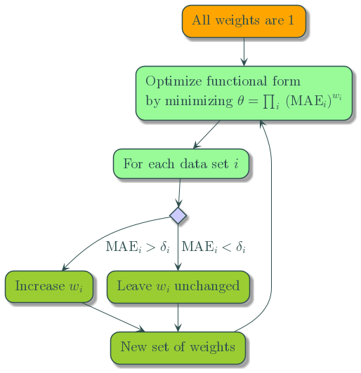
Figure 2: Adjustment of the weights in the functional optimization, see Eq. (24). Here, $\delta_{i}$ are thresholds for each data set, while $w_{i}$ are the corresponding weights. The evaluation was done 100 times and the best weights, i.e., the best compromise for all nonSCF MAEs, was taken for further evaluation.

As a starting point, all weights were set to 1. The functional form is optimized, and the nonSCF predictions of the MAE for each data set are computed. If an MAE is beyond a predefined threshold, the weight for the data set is increased (see SI, Tab. ST1 for values). After this modification, the functional is optimized once again and the process starts anew. This optimization route was performed 100 times. The best possible weights, i.e., the best compromise between all predicted MAEs, were adjusted to minimize the errors further. The final weights (see SI, Tab. ST2) were then taken to obtain the optimal $c_{ij}$ (see SI, Tab. ST3).

V.4 Enforce smoothness

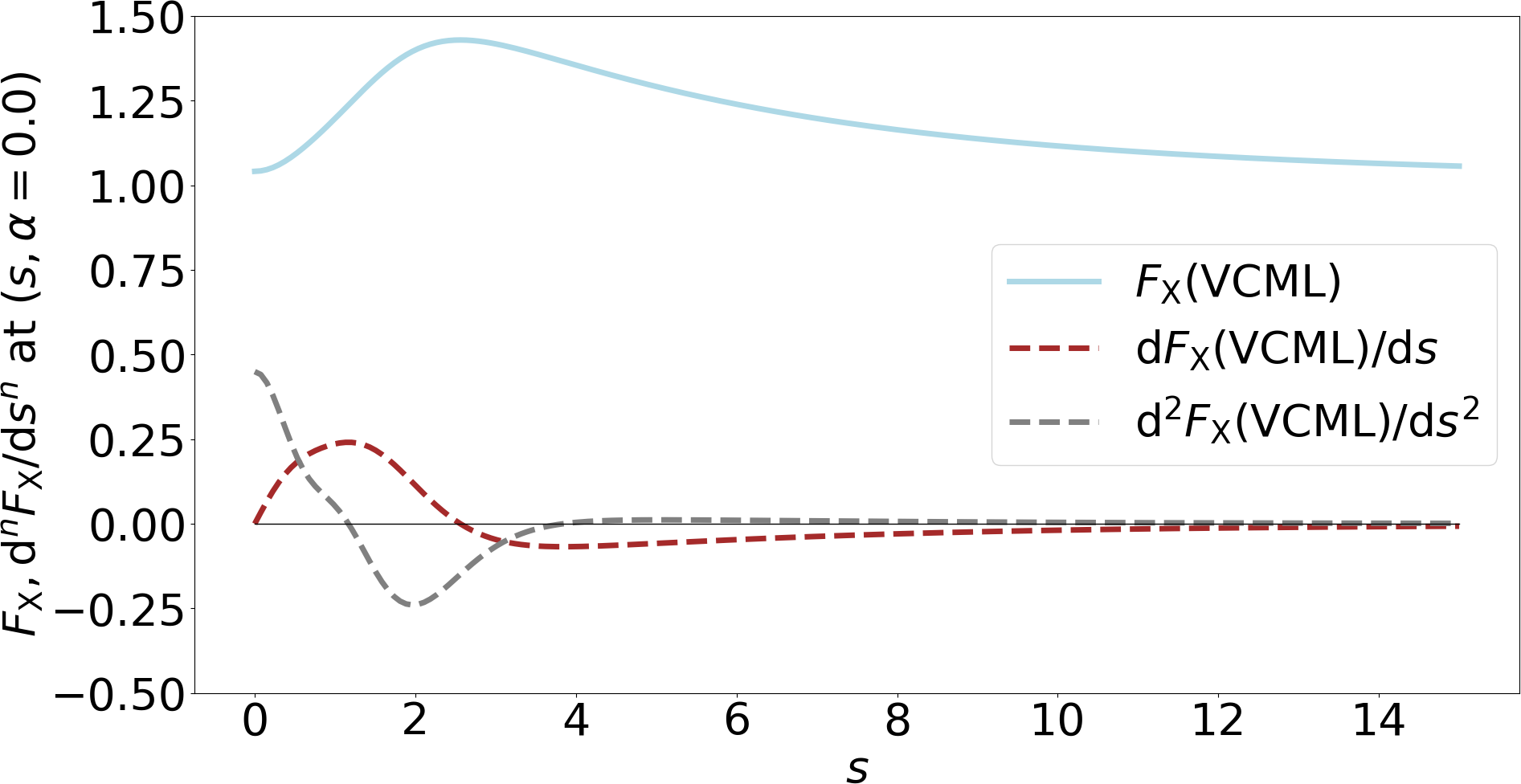
Figure 3: $F_{\text{X}}$ as well as the first and second derivative of $F_{\text{X}}$ with respect to the reduced density gradient $s$ at $\alpha=0$ for VCML, which is the semilocal exchange part of VCML-rVV10. While $\text{d}F_{\text{X}}/\text{d}s$ shows exactly one sign change, $\text{d}^{2}F_{\text{X}}/\text{d}s^{2}$ shows two. As such, the regularizations regarding the sign changes of derivatives of $F_{\text{X}}$ work as intended. This enforces a certain smoothness of the functional.

To avoid oscillatory behavior of high-order polynomial fits, the $F_{\text{X}}$ is enforced to be smooth. The number of sign changes beyond given thresholds in the first and second derivatives of $F_{\text{X}}$ with respect to $s$ and $\alpha$ is penalized. A penalty is added if there is more than one sign change in the first derivatives. This allows the exchange enhancement factor to have one extremum in $s$ for a given $\alpha$. Further, a penalty is applied if there are more than two sign changes in the second derivatives. With that, the functional should go smoothly towards and away from the extremum. Derivatives of the Legendre polynomials used to expand $F_{\text{X}}$ are efficiently computed via recursion. The zeros of the resulting polynomials corresponding to the first and second derivatives are obtained as the eigenvalues of the companion matrices. This sign-change penalty technique enables us to enforce smoothness of $F_{\text{X}}$ in a computationally straightforward way. As an example, the first and second derivative of $F_{\text{X}}$ with respect to $s$ at $\alpha=0$ (single orbital limit) for VCML, the semilocal exchange part of VCML-rVV10, are shown in Fig. 3. As one can see, the proposed regularizations work as intended in making the functional smooth. Note that there are different mathematical forms of $F_{\text{X}}$ not based on polynomial expansions allowing for other techniques to enforce constraints and smoothness.¹⁹

V.5 Summary of entire procedure to obtain VCML

Fig. 4 summarizes the fitting procedure.

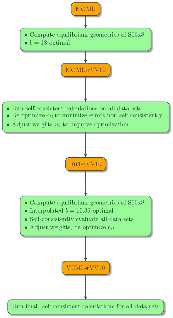
Figure 4: Procedure to arrive at the VCML-rVV10 functional form. Starting from MCML, the optimal $b$ parameter of the rVV10 methodology is determined. The resulting MCML-rVV10 functional is used to compute all data sets self-consistently. Based on these results, the functional form was adjusted according to the minimization of Eq. (24). The adjustment of the weights is illustrated in Fig. 2. This results in an intermediate functional form, called Fit1-rVV10. For this functional, the $b$ parameter was re-optimized, and all data sets were re-calculated self-consistently. Finally, the functional form was re-optimized once again, resulting in VCML-rVV10. Due to careful consideration of the errors in S66x8 as described in the SI, Sec. 3, the $b$ parameter needed no further optimization.

It starts by taking the MCML functional. An optimal $b$ parameter for rVV10 is determined. For this, the equilibrium structures of S66x8 and their resulting errors were used. Various $b$ values were analyzed, ranging from 3 to 25 with a stepsize of 1. The optimal value, $b=18$, defines MCML-rVV10. After calculating all data sets (see Section IV) with MCML-rVV10, the functional form was re-optimized using the methodology outlined above. This led to an intermediate functional form, Fit1-rVV10.

For Fit1-rVV10, the $b$ value was re-optimized, using a range of $b$ values between 13 and 21 and a smaller stepsize of 0.25. From this search, an optimal $b$ value of 15.35 was interpolated. After that, all properties of all data sets were recalculated self-consistently. The resulting data is used once again to re-optimize the functional form. For this final optimization, we made sure that the nonSCF errors for the S66x8 remain small, see SI, Sec. 3 for further details. This avoids re-optimizing the $b$ parameter. Accordingly, the $b$ parameter for the final VCML-rVV10 functional is also 15.35.

In summary, the $b$ parameter as well as the functional form were optimized twice, starting from MCML. Given an overall good performance of VCML-rVV10 in comparison to MCML-rVV10 and other functionals (see Sec. VI), we terminate the functional optimization loop here.

VI Results and discussion

VI.1 Comparing $F_{\text{X}}$ to other functionals

The $F_{\text{X}}$ of MS2, SCAN, MCML as well as the new VCML are plotted in Fig. 5. In certain regions of $s$ and $\alpha$, VCML is similar to MS2, e.g., $F_{\text{X}}(s=0,\alpha>0.5)$. On the other hand, VCML is similar to SCAN for $F_{\text{X}}(s>8,\alpha=1)$. While the VCML and MCML exchange enhancement factor are similar for low reduced density gradients, the VCML exchange enhancement is markedly larger at reduced density gradients $s\gtrsim 2$. The maximum value of VCML’s $F_{\text{X}}$ is 1.432, which is well below the Lieb-Oxford bound of 1.804.¹⁵ Note that remaining below this bound was not explicitly enforced, nor was the decaying behavior with increasing $s$.

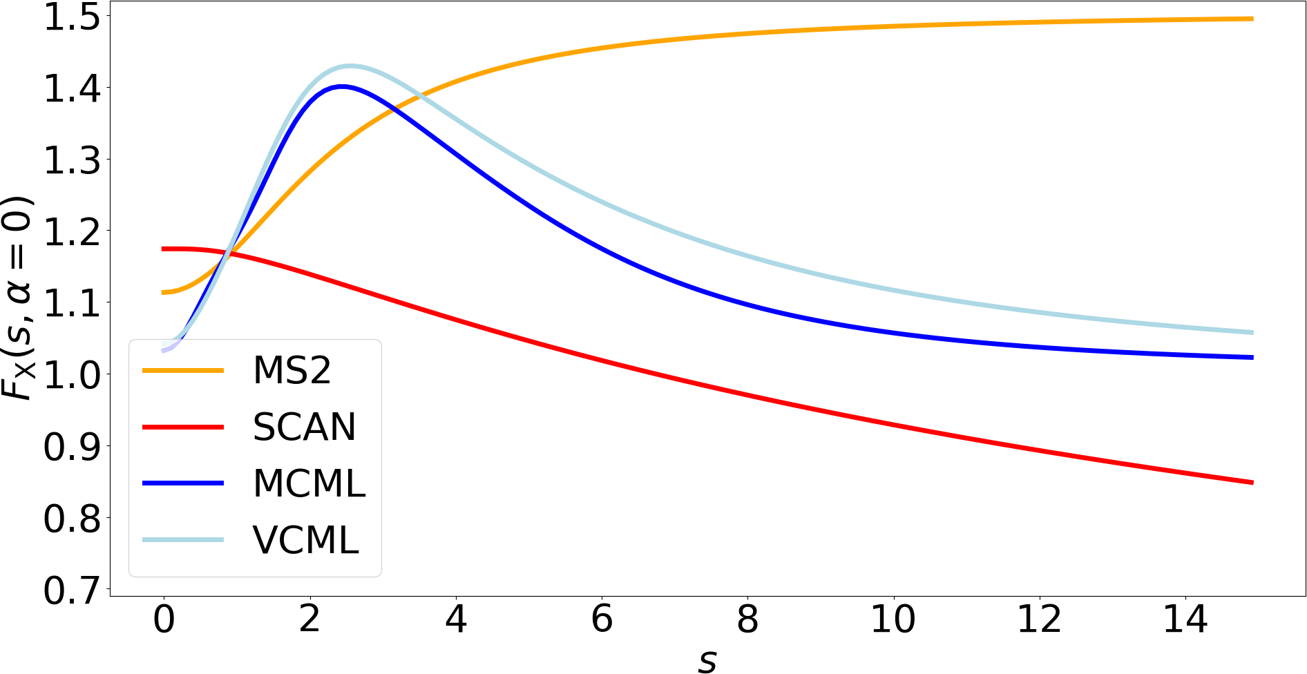
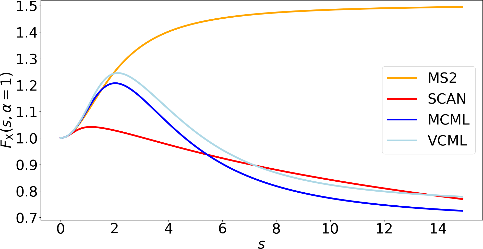
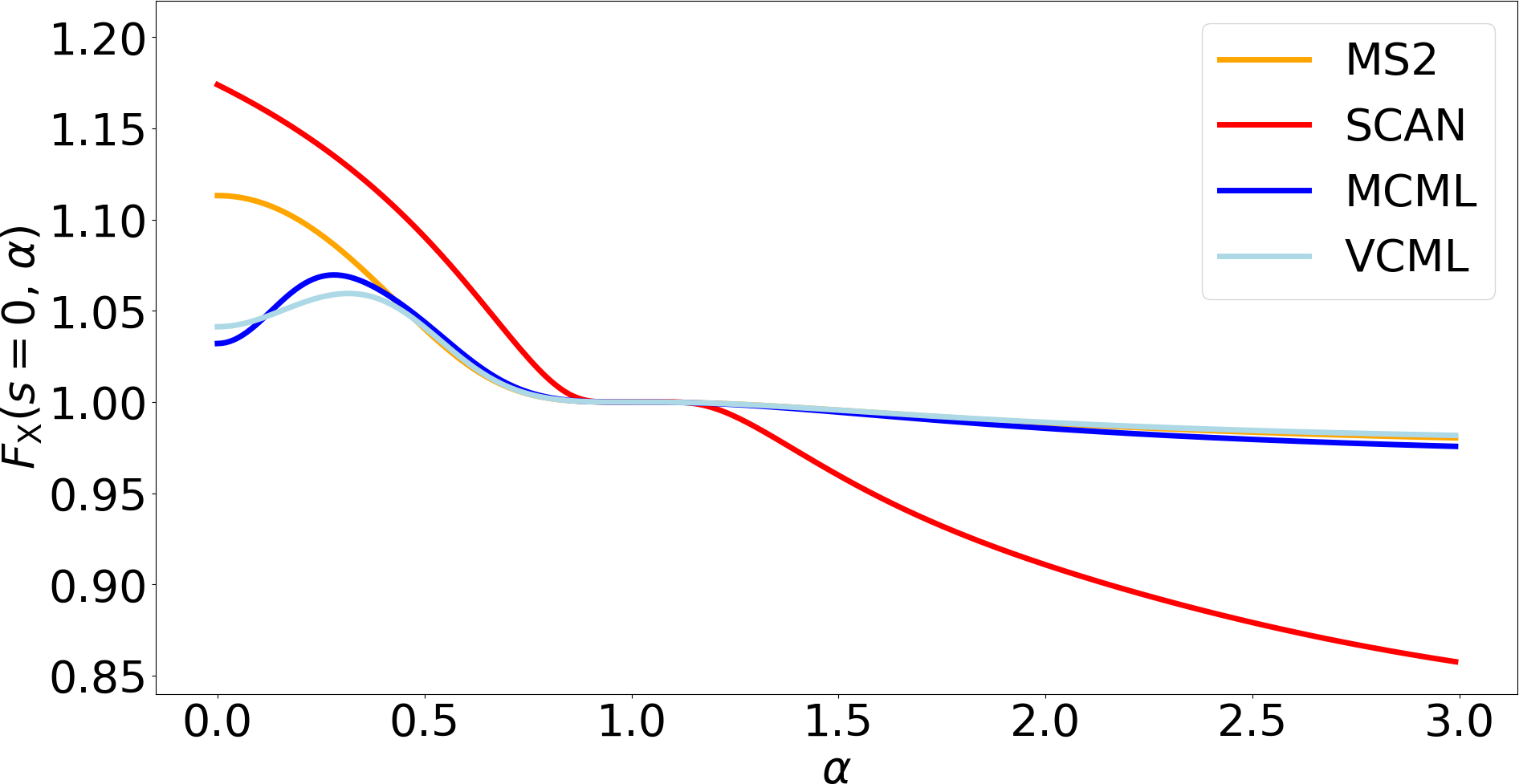
Figure 5: Exchange enhancement factor for different regimes of $s$ and $\alpha$ for MS2, SCAN, MCML and VCML. Top: $F_{\text{X}}$ for $\alpha=0$ over a range of $s$. Middle: $F_{\text{X}}$ for $\alpha=1$ over a range of $s$. Bottom: $F_{\text{X}}$ for $s=0$ over a range of $\alpha$. One can clearly see that $F_{\text{X}}(s=0,\alpha=1)=1$; this is the LDA limit that is fulfilled by all the presented functionals, as is the curvature in this point given by the exchange gradient expansion.

VI.2 Performance on data sets

A summary of the MAEs for all data sets using the functionals described in the main text is shown in Fig. 6. For all values of MEs and MAEs see SI, Tab. ST4 and ST5.

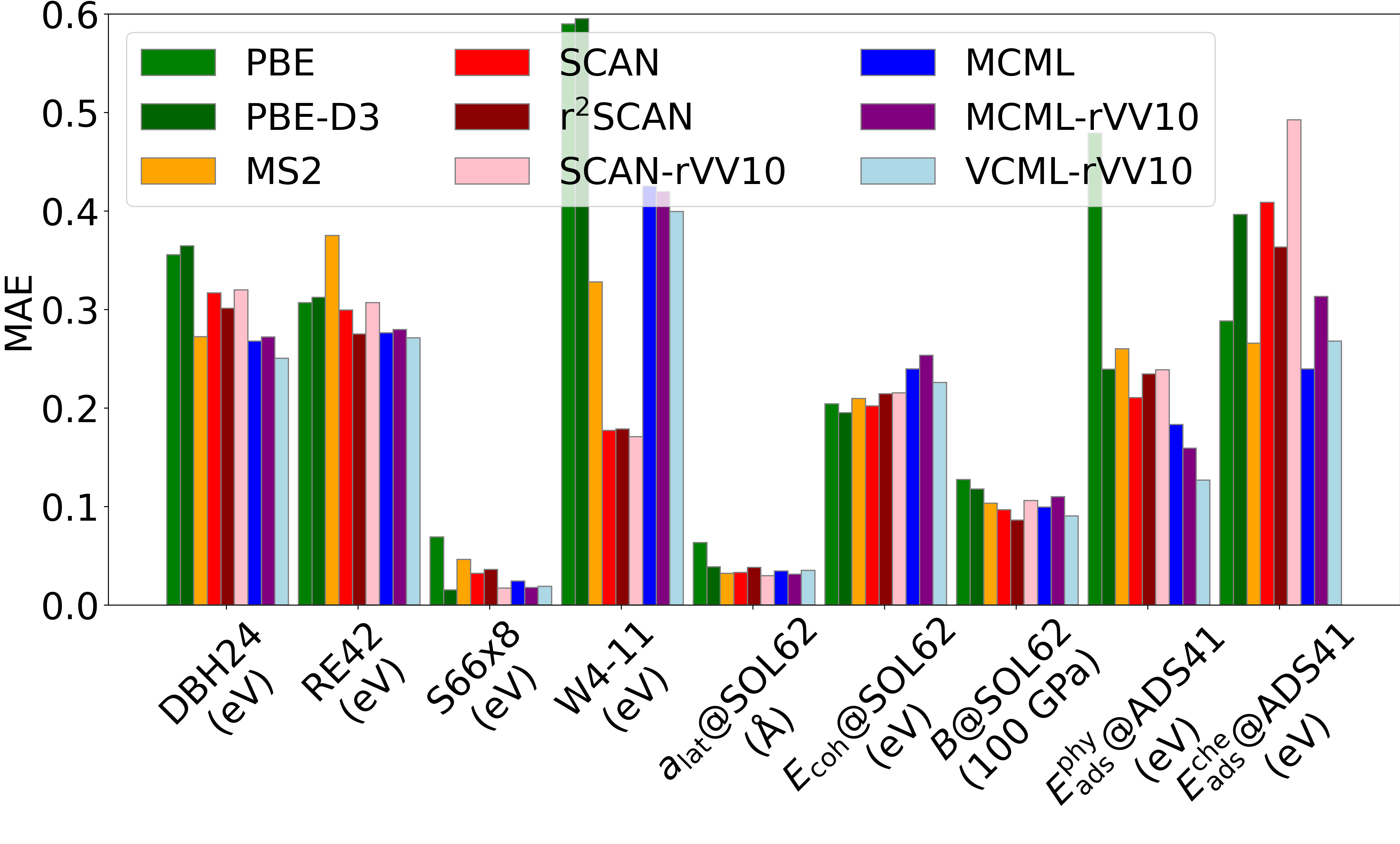
Figure 6: Comparison of the mean absolute errors (MAEs) in the different data sets for all employed functionals. The units per data set are provided. Detailed plots with all errors per data set of all functionals can be found in the SI, Fig. SF2-13.

Overall, our VCML-rVV10 functional shows small errors for a range of physical properties. This confirms that we have created a multi-purpose functional. It should be noted that our fitting approach favors errors of certain data sets over others. There is always a compromise between making a specific error better, while making some other error(s) worse. Accordingly, the improvements seen for VCML-rVV10 over, e.g., MCML is the best overall compromise we found. For a more detailed analysis of the resulting errors, see below.

For DBH24

VCML-rVV10 performs best, followed by MCML. Barrier heights are poorly described in DFT approximations based on semi-local exchange; all functionals produce a relatively large error for the barriers due to large self-interaction error in the regime of stretched bonds.⁴⁹

For RE42

again VCML-rVV10 performs best, followed by r²SCAN. Thus, the description of the reaction between molecules is described well by VCML-rVV10.

For S66x8

SCAN-rVV10, MCML-rVV10 and VCML-rVV10 perform similarly, and clearly outperform any functional that does not include any vdW correction. This is a proof of concept that the rVV10 methodology works as intended. It furthermore shows that refitting the functional form from MCML to VCML did not diminish the prediction of these non-covalent interactions.

For W4-11

we find a poor performance of VCML-rVV10. As noted in Brown et al.,¹⁸ MCML performs worse on atomization energies than other tested functionals. This is confirmed as seen in Fig. 6. With VCML-rVV10, we actually improve the MAE by about 20 meV. However, we find there is a trade-off especially between $E_{\textrm{ads}}^{\textrm{che}}$@ADS41 and $E_{\textrm{coh}}$@SOL62. Atomization energies of solids and molecules cannot be improved further here without deteriorating the description of surface chemistry.

For SOL62

VCML-rVV10 performs very similar for $a_{\text{lat}}$@SOL62 compared to the other meta-GGAs. All of them perform well on lattice constants, with differences in their MAE of at most 0.005 Å.

Furthermore, VCML-rVV10 outperforms MCML as well as MCML-rVV10 for $E_{\text{coh}}$@SOL62. MCML is not an optimal functional for the description of cohesive energies;¹⁸ adding rVV10 on-top makes matters worse. Due to the fact that we reshaped the functional form, we arrive at an MAE which is only about 10 meV worse than SCAN-rVV10, but already 15 meV better than MCML.

For $B$@SOL62, VCML-rVV10 is the second best functional after r²SCAN, clearly outperforming the other functionals that employ vdW-corrections in the form of rVV10.

Overall, VCML-rVV10 performs well for solids regarding the three properties studied here. We do not diminish the performance on the solid properties and thus maintain the multi-purpose character of VCML-rVV10.

For ADS41

we obtain the smallest errors in the physisorption-dominated systems using VCML-rVV10, outperforming MCML-rVV10 and SCAN-rVV10. All functionals without rVV10 have, unsurprisingly, larger errors.

For chemisorption-dominated systems, VCML-rVV10 performs significantly better than all other vdW-supplemented functionals considered here; the resulting MAE is a good as MS2. As such, VCML-rVV10 is the second best functional (together with MS2) for these systems. Only MCML gives smaller errors, at the price of not explicitly accounting for dispersion forces.

For all data sets it is clear that only adding rVV10 on-top of MCML, i.e., MCML-rVV10, does not provide a good vdW-meta-GGA functional. Reshaping the functional form based on a given vdW correction drastically improves the performance of the functional, making it applicable to a wide range of physical properties while also treating non-local interactions via the rVV10 methodology.

VI.3 Graphene on Ni

To test VCML-rVV10 outside of the training data shown in Fig. 6, we calculated the interaction energy of graphene on a Ni(111) surface. Previous theoretical investigations found that there likely are two distinct minima.^{50, 51} These minima can be characterized as a chemisorption minimum at a smaller distance between graphene and Ni, and a physisorption minimum at a larger distance. In experiments, usually only the first minimum is found.⁵¹ In the literature, reference calculations have been carried out using the random phase approximation (RPA).⁵² It has been noted that the RPA is likely to underestimate the chemisorption minimum.^{50, 51} This can be seen when comparing to experimental estimates,⁵¹ which are shown as the grey cross in Fig. 7. The second minimum, on the other hand, is likely captured well by the RPA.

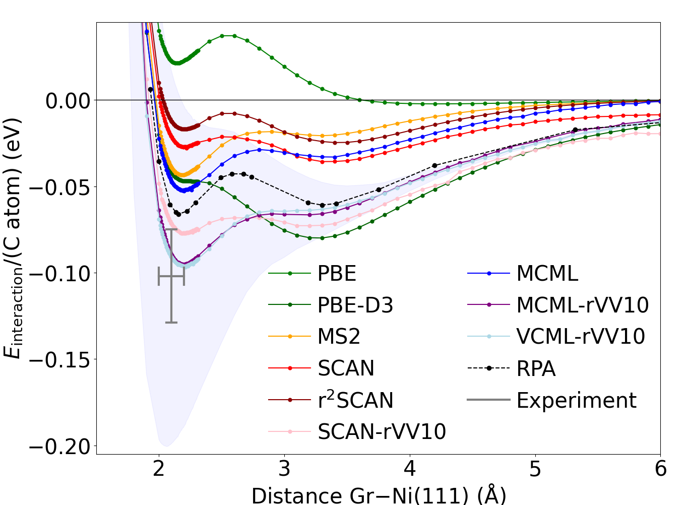
Figure 7: Interaction energy of graphene on Ni(111) at several distances using different functionals. Only MCML-rVV10 and VCML-rVV10 capture the experimental value of the first minimum⁵¹ correctly. VCML-rVV10 is also energetically very close to the RPA⁵² for the second, physisorption-dominated minimum. The shaded area indicates $\pm 1$ standard deviation calculated from a Bayesian ensemble of 5000 perturbations to the VCML exchange enhancement.

In Fig. 7, we compare the interaction energy per C atom calculated with all functionals considered in this article. As a note, the optimal lattice constant for Ni for each functional was employed. Of all the functionals, only MCML-rVV10 and VCML-rVV10 describe the energy of the first minimum accurately, with VCML-rVV10 being within 6 meV of the average estimate of the experimental chemisorption energy.⁵¹ All other functionals underestimate this minimum or predict it to be as strongly bound as the physisorbed case. Further, VCML-rVV10 is energetically closest to RPA for the second minimum. As a note, VCML-rVV10 and MCML-rVV10 are the only functionals that are very close, within 5 meV, to the RPA values at larger distances. As such, VCML-rVV10 describes both chemisorption and physisorption accurately, indicating a well-balanced functional.

The decomposition of $E_{\text{X}}$ into contributions from the different Legendre polynomial products in the expansion of the exchange-enhancement factor $F_{\text{X}}$ allows for efficient non-self-consistent estimates of changes in $E_{\text{X}}$ due to perturbations of $F_{\text{X}}$. Following the strategy outlined in Refs. ¹⁸ and ⁵³, we use such perturbations to estimate the uncertainty in the interaction energy of graphene with Ni(111) in the example above using Bayesian inference. Perturbations to $F_{\text{X}}$ are drawn randomly with a probability $\propto\exp(-\text{Loss}_{2}(\theta)/\tau)$. $\text{Loss}_{2}(\theta)$ is the squared error with respect to the reference fitting data as a function of the parameters $\theta$ defining $F_{\text{X}}$ under fulfillment of the constraints Eqs. (21), (22), and (23). For the computation of $\text{Loss}_{2}(\theta)$, the energies in each data set are normalized such that the MAE of each data set is one. The fictitious temperature $\tau$ is determined such that the residual fitting error of VCML-rVV10 is reproduced (see Ref. ¹⁸ for further details on the implementation of the error estimates). The predicted uncertainty for the interaction of graphene with Ni(111) is shown as the shaded area in Fig. 7. The Bayesian error estimate for the chemisorption energy is about 0.2 eV, which is consistent with the residual error on the chemisorption benchmark data, see Fig. 6. The ensemble error covers all stable adsorption minima. The predicted error vanishes at larger distances, where VCML-rVV10 and RPA agree very well.

VII Conclusion

In this work, a new meta-GGA van der Waals (vdW) exchange-correlation (XC) functional called VCML-rVV10 is introduced. This functional is obtained from a simultaneous optimization of both semi-local exchange via a multi-parameter model and non-local correlation of rVV10-type. VCML-rVV10 was trained on a number of data sets representing several chemical and physical properties. This enables the multi-purpose character of the functional. In addition, several constraints of the exact XC functional were enforced for physicality of the VCML-rVV10 model.

The newly introduced functional shows good performance in comparison to all other functionals tested, some of which also employing the rVV10 methodology. It also performs very well on the description of graphene on Ni(111), which was not included in the training data. This benchmark system requires a balanced, accurate description of surface physisorption as well as chemisorption.

In the future, the introduced methodology of simultaneous, regularized optimization of several parts of an XC functional could be extended to hybrid functionals, where a to-be-fitted amount of screened exact exchange would be admixed to the to-be-optimized density functional.

VIII Acknowledgement

This research was supported by the U.S. Department of Energy, Office of Science, Office of Basic Energy Sciences, Chemical Sciences, Geosciences, and Biosciences Division, Catalysis Science Program to the SUNCAT Center for Interface Science and Catalysis. We greatly appreciate the help of James Furness for providing a patch for VASP making r²SCAN available.

IX Supporting Information

• Further details for rVV10

• Visualization of transformation of $s$ and $\alpha$

• Details of the functional fitting procedure

• Fitting weights

• Final coefficients $c_{ij}$

• Tables for mean and mean absolute errors

• Tables with all calculated values

• Figures with all evaluated errors

X Data availability statement

All data, including the VASP inputs/outputs as well as all calculated values, is available at GitLab https://gitlab.com/kaitrepte/vcml_data. The ADS41 adsorbate system structures can also be found on catalysis-hub,⁵⁴ see https://www.catalysis-hub.org/publications/KaiData-driven2022. VCML-rVV10 is available in libXC,⁵⁵ see https://github.com/ElectronicStructureLibrary/libxc. An alternative FORTRAN routine for evaluation of the VCML exchange energy can be found at https://github.com/vossgroup/CML.

References

- Hohenberg and Kohn 1964 P. Hohenberg and W. Kohn. Inhomogeneous Electron Gas. Phys. Rev., 136:B864–B871, 1964. doi: 10.1103/PhysRev.136.B864.
- Kohn and Sham 1965 W. Kohn and L. J. Sham. Self-Consistent Equations Including Exchange and Correlation Effects. Phys. Rev., 140:A1133, 1965. doi: 10.1103/PhysRev.140.A1133.
- Kohn et al. 1996 W. Kohn, A. D. Becke, and R. G. Parr. Density Functional Theory of Electronic Structure. J. Phys. Chem., 100:12974, 1996. doi: 10.1021/jp960669l.
- Burke 2012 K. Burke. Perspective on density functional theory. J. Chem. Phys., 136:150901, 2012. doi: 10.1063/1.4704546.
- Mardirossian and Head-Gordon 2017 N. Mardirossian and M. Head-Gordon. Thirty years of density functional theory in computational chemistry: an overview and extensive assessment of 200 density functionals. Mol. Phys., 115:2315–2372, 2017. doi: 10.1080/00268976.2017.1333644.
- Becke 1993 A. D. Becke. Density‐functional thermochemistry. III. The role of exact exchange. J. Chem. Phys., 98:5648–5652, 1993. doi: 10.1063/1.464913.
- Zhao et al. 2005 Y. Zhao, N. E. Schultz, and D. G. Truhlar. Exchange-correlation functional with broad accuracy for metallic and nonmetallic compounds, kinetics, and noncovalent interactions. J. Chem. Phys., 123:161103, 2005. doi: 10.1063/1.2126975.
- Peverati and Truhlar 2014 R. Peverati and D. G. Truhlar. Quest for a universal density functional: the accuracy of density functionals across a broad spectrum of databases in chemistry and physics. Philos. Trans. R. Soc. A, 372:20120476, 2014. doi: 10.1098/rsta.2012.0476.
- Mardirossian and Head-Gordon 2014 N. Mardirossian and M. Head-Gordon. B97X-V: A 10-parameter, range-separated hybrid, generalized gradient approximation density functional with nonlocal correlation, designed by a survival-of-the-fittest strategy. Phys. Chem. Chem. Phys., 16:9904–9924, 2014. doi: 10.1039/C3CP54374A.
- Perdew et al. 1996 J. P. Perdew, K. Burke, and M. Ernzerhof. Generalized Gradient Approximation Made Simple. Phys. Rev. Lett., 77:3865–3868, 1996. doi: 10.1103/PhysRevLett.77.3865.
- Perdew et al. 2008 J. P. Perdew, A. Ruzsinszky, G. I. Csonka, O. A. Vydrov, G. E. Scuseria, L. A. Constantin, X. Zhou, and K. Burke. Restoring the Density-Gradient Expansion for Exchange in Solids and Surfaces. Phys. Rev. Lett., 100:136406, 2008. doi: 10.1103/PhysRevLett.100.136406.
- Sun et al. 2015 J. Sun, A. Ruzsinszky, and J. P. Perdew. Strongly Constrained and Appropriately Normed Semilocal Density Functional. Phys. Rev. Lett., 115:036402, 2015. doi: 10.1103/PhysRevLett.115.036402.
- Garza et al. 2018 A. J. Garza, A. T. Bell, and M. Head-Gordon. Nonempirical Meta-Generalized Gradient Approximations for Modeling Chemisorption at Metal Surfaces. J. Chem. Theory Comput., 14:3083–3090, 2018. doi: 10.1021/acs.jctc.8b00288.
- Furness et al. 2020 J. W. Furness, A. D. Kaplan, J. Ning, J. P. Perdew, and J. Sun. Accurate and Numerically Efficient r2SCAN Meta-Generalized Gradient Approximation. J. Phys. Chem. Lett., 11:8208–8215, 2020. doi: 10.1021/acs.jpclett.0c02405.
- Perdew et al. 2014 J. P. Perdew, A. Ruzsinszky, J. Sun, and K. Burke. Gedanken densities and exact constraints in density functional theory. J. Chem. Phys., 140:18A533, 2014. doi: 10.1063/1.4870763.
- Bokdam et al. 2017 M. Bokdam, J. Lahnsteiner, B. Ramberger, T. Schäfer, and G. Kresse. Assessing Density Functionals Using Many Body Theory for Hybrid Perovskites. Phys. Rev. Lett., 119:145501, 2017. doi: 10.1103/PhysRevLett.119.145501.
- Zhang et al. 2018 G.-X. Zhang, A. M. Reilly, A. Tkatchenko, and M. Scheffler. Performance of various density-functional approximations for cohesive properties of 64 bulk solids. New J. Phys., 20:063020, 2018. doi: 10.1088/1367-2630/aac7f0.
- Brown et al. 2021 K. Brown, Y. Maimaiti, K. Trepte, T. Bligaard, and J. Voss. MCML: Combining physical constraints with experimental data for a multi-purpose meta-generalized gradient approximation. J. Comput. Chem., 42:2004–2013, 2021. doi: https://doi.org/10.1002/jcc.26732.
- Sparrow et al. 2021 Z. M. Sparrow, B. G. Ernst, T. K. Quady, and R. A. DiStasio Jr. CASE21: Uniting Non-Empirical and Semi-Empirical Density Functional Approximation Strategies using Constraint-Based Regularization. arXiv, 2109.12560, 2021.
- Zhao et al. 2006 Y. Zhao, N. E. Schultz, and D. G. Truhlar. Design of Density Functionals by Combining the Method of Constraint Satisfaction with Parametrization for Thermochemistry, Thermochemical Kinetics, and Noncovalent Interactions. J. Chem. Theory Comput., 2:364–382, 2006. doi: 10.1021/ct0502763.
- Duanmu and Truhlar 2017 K. Duanmu and D. G. Truhlar. Validation of Density Functionals for Adsorption Energies on Transition Metal Surfaces. J. Chem. Theory Comput., 13:835–842, 2017. doi: 10.1021/acs.jctc.6b01156.
- Sharada et al. 2019 S. M. Sharada, R. K. B. Karlsson, Y. Maimaiti, J. Voss, and T. Bligaard. Adsorption on transition metal surfaces: Transferability and accuracy of DFT using the ADS41 dataset. Phys. Rev. B, 100:035439, 2019. doi: 10.1103/PhysRevB.100.035439.
- Wellendorff et al. 2012 J. Wellendorff, K. T. Lundgaard, A. Møgelhøj, V. Petzold, D. D. Landis, J. K. Nørskov, T. Bligaard, and K. W. Jacobsen. Density functionals for surface science: Exchange-correlation model development with Bayesian error estimation. Phys. Rev. B, 85:235149, 2012. doi: 10.1103/PhysRevB.85.235149.
- Klimeš et al. 2009 J. Klimeš, D. R. Bowler, and A. Michaelides. Chemical accuracy for the van der Waals density functional. J. Phys.: Condens. Matter, 22:022201, 2009. doi: 10.1088/0953-8984/22/2/022201.
- Vydrov and Van Voorhis 2010 O. A. Vydrov and T. Van Voorhis. Nonlocal van der Waals density functional: The simpler the better. J. Chem. Phys., 133:244103, 2010. doi: 10.1063/1.3521275.
- Sabatini et al. 2013 R. Sabatini, T. Gorni, and S. de Gironcoli. Nonlocal van der Waals density functional made simple and efficient. Phys. Rev. B, 87:041108, 2013. doi: 10.1103/PhysRevB.87.041108.
- Peng et al. 2016 H. Peng, Z.-H. Yang, J. P. Perdew, and J. Sun. Versatile van der Waals Density Functional Based on a Meta-Generalized Gradient Approximation. Phys. Rev. X, 6:041005, 2016. doi: 10.1103/PhysRevX.6.041005.
- Perdew et al. 2009 J. P. Perdew, A. Ruzsinszky, G. I. Csonka, L. A. Constantin, and J. Sun. Workhorse Semilocal Density Functional for Condensed Matter Physics and Quantum Chemistry. Phys. Rev. Lett., 103:026403, 2009. doi: 10.1103/PhysRevLett.103.026403.
- Perdew and Schmidt 2001 J. P. Perdew and K. Schmidt. Jacob’s ladder of density functional approximations for the exchange-correlation energy. AIP Conf. Proc., 577:1–20, 2001. doi: 10.1063/1.1390175.
- Kresse and Furthmüller 1993 G. Kresse and J. Furthmüller. Efficient iterative schemes for ab initio total-energy calculations using a plane-wave basis set. Phys. Rev. B, 54:11169, 1993. doi: 10.1103/PhysRevB.54.11169.
- Blöchl 1994 P. E. Blöchl. Projector augmented-wave method. Phys. Rev. B, 50:17953, 1994. doi: 10.1103/PhysRevB.50.17953.
- Kresse and Joubert 1999 G. Kresse and D. Joubert. From ultrasoft pseudopotentials to the projector augmented-wave method. Phys. Rev. B, 59:1758, 1999. doi: 10.1103/PhysRevB.59.1758.
- Grimme et al. 2010 S. Grimme, J. Antony, S. Ehrlich, and H. Krieg. A consistent and accurate ab initio parametrization of density functional dispersion correction (DFT-D) for the 94 elements H-Pu. J. Chem. Phys., 132:154104, 2010. doi: 10.1063/1.3382344.
- Sun et al. 2013 J. Sun, R. Haunschild, B. Xiao, I. W. Bulik, G. E. Scuseria, and J. P. Perdew. Semilocal and hybrid meta-generalized gradient approximations based on the understanding of the kinetic-energy-density dependence. J. Chem. Phys., 138:044113, 2013. doi: 10.1063/1.4789414.
- Zheng et al. 2007 J. Zheng, Y. Zhao, and D. G. Truhlar. Representative Benchmark Suites for Barrier Heights of Diverse Reaction Types and Assessment of Electronic Structure Methods for Thermochemical Kinetics. J. Chem. Theory Comput., 3:569, 2007. doi: 10.1021/ct600281g.
- Zheng et al. 2009 J. Zheng, Y. Zhao, and D. G. Truhlar. The DBH24/08 Database and Its Use to Assess Electronic Structure Model Chemistries for Chemical Reaction Barrier Heights. J. Chem. Theory Comput., 5:808–821, 2009. doi: 10.1021/ct800568m.
- Curtiss et al. 1997 L. A. Curtiss, K. Raghavachari, P. C. Redfern, and J. A. Pople. Assessment of Gaussian-2 and density functional theories for the computation of enthalpies of formation. J. Chem. Phys., 106:1063–1079, 1997. doi: 10.1063/1.473182.
- Rezac et al. 2011 J. Rezac, K. E. Riley, and P. Hobza. S66: A Well-balanced Database of Benchmark Interaction Energies Relevant to Biomolecular Structures. J. Chem. Theory Comput., 7:2427–2438, 2011. doi: 10.1021/ct2002946.
- Brauer et al. 2016 B. Brauer, M. K. Kesharwani, S. Kozuch, and J. M. L. Martin. The S66x8 benchmark for noncovalent interactions revisited: explicitly correlated ab initio methods and density functional theory. Phys. Chem. Chem. Phys., 18:20905–20925, 2016. doi: 10.1039/C6CP00688D.
- Karton et al. 2011 A. Karton, S. Daon, and J. M. L. Martin. W4-11: A high-confidence benchmark dataset for computational thermochemistry derived from first-principles W4 data. Chem. Phys. Lett., 510:165–178, 2011. doi: https://doi.org/10.1016/j.cplett.2011.05.007.
- Alchagirov et al. 2001 A. B. Alchagirov, J. P. Perdew, J. C. Boettger, R. C. Albers, and C. Fiolhais. Energy and pressure versus volume: Equations of state motivated by the stabilized jellium model. Phys. Rev. B, 63:224115, 2001. doi: 10.1103/PhysRevB.63.224115.
- Wellendorff et al. 2015 J. Wellendorff, T. L. Silbaugh, D. Garcia-Pintos, J. K. Nørskov, T. Bligaard, F. Studt, and C. T. Campbell. A benchmark database for adsorption bond energies to transition metal surfaces and comparison to selected DFT functionals. Surf. Sci., 640:36–44, 2015. doi: https://doi.org/10.1016/j.susc.2015.03.023.
- Lieb and Oxford 1981 E. H. Lieb and S. Oxford. Improved lower bound on the indirect Coulomb energy. Int. J. Quantum Chem., 19:427, 1981. doi: https://doi.org/10.1002/qua.560190306.
- Perdew 1991 J. P Perdew. Unified theory of exchange and correlation beyond the local density approximation. In P. Ziesche and H. Eschrig, editors, Electronic Structure of Solids ’91, volume 17 of Physical Research, pages 11–20, Berlin, 1991. Akademie Verlag.
- Antoniewicz and Kleinman 1985 P. R. Antoniewicz and L. Kleinman. Kohn-Sham exchange potential exact to first order in (K)/. Phys. Rev. B, 31:6779, 1985. doi: 10.1103/PhysRevB.31.6779.
- Nelder and Mead 1965 J. A. Nelder and R. Mead. A Simplex Method for Function Minimization. Comput. J., 7:308, 1965. doi: 10.1093/comjnl/7.4.308.
- Gao and Han 2012 F. Gao and L. Han. Implementing the Nelder-Mead simplex algorithm with adaptive parameters. Comput. Optim. Appl., 51:259, 2012. doi: 10.1007/s10589-010-9329-3.
- Virtanen et al. 2020 P. Virtanen, R. Gommers, T. E. Oliphant, M. Haberland, T. Reddy, D. Cournapeau, E. Burovski, P. Peterson, W. Weckesser, J. Bright, S. J. van der Walt, M. Brett, J. Wilson, K. J. Millman, N. Mayorov, A. R. J. Nelson, E. Jones, R. Kern, E. Larson, C. J. Carey, İ. Polat, Y. Feng, E. W. Moore, J. VanderPlas, D. Laxalde, J. Perktold, R. Cimrman, I. Henriksen, E. A. Quintero, C. R. Harris, A. M. Archibald, A. H. Ribeiro, F. Pedregosa, P. van Mulbregt, and SciPy 1.0 Contributors. SciPy 1.0: Fundamental algorithms for scientific computing in Python. Nat. Methods, 17:261, 2020. doi: 10.1038/s41592-019-0686-2.
- Shahi et al. 2019 C. Shahi, P. Bhattarai, K. Wagle, B. Santra, S. Schwalbe, T. Hahn, J. Kortus, K. A. Jackson, J. E. Peralta, K. Trepte, S. Lehtola, N. K. Nepal, H. Myneni, B. Neupane, S. Adhikari, A. Ruzsinszky, Y. Yamamoto, T. Baruah, R. R. Zope, and J. P. Perdew. Stretched or noded orbital densities and self-interaction correction in density functional theory. J. Chem. Phys., 150:174102, 2019. doi: 10.1063/1.5087065.
- Olsen and Thygesen 2013 T. Olsen and K. S. Thygesen. Random phase approximation applied to solids, molecules, and graphene-metal interfaces: From van der Waals to covalent bonding. Phys. Rev. B, 87:075111, 2013. doi: 10.1103/PhysRevB.87.075111.
- Shepard and Smeu 2019 S. Shepard and M. Smeu. First principles study of graphene on metals with the SCAN and SCAN+rVV10 functionals. J. Chem. Phys., 150:154702, 2019. doi: 10.1063/1.5046855.
- Mittendorfer et al. 2011 F. Mittendorfer, A. Garhofer, J. Redinger, J. Klimeš, J. Harl, and G. Kresse. Graphene on Ni(111): Strong interaction and weak adsorption. Phys. Rev. B, 84:201401, 2011. doi: 10.1103/PhysRevB.84.201401.
- Mortensen et al. 2005 J. J. Mortensen, K. Kaasbjerg, S. L. Frederiksen, J. K. Nørskov, J. P. Sethna, and K. W. Jacobsen. Bayesian error estimation in density-functional theory. Phys. Rev. Lett., 95:216401, 2005. doi: 10.1103/PhysRevLett.95.216401.
- Winther et al. 2019 K. T. Winther, M. J. Hoffmann, J. R. Boes, O. Mamun, M. Bajdich, and T. Bligaard. Catalysis-hub. org, an open electronic structure database for surface reactions. Sci. data, 6(1):1–10, 2019. doi: 10.1038/s41597-019-0081-y.
- Lehtola et al. 2018 S. Lehtola, C. Steigemann, M. J. T. Oliveira, and M. A. L. Marques. Recent developments in LIBXC – A comprehensive library of functionals for density functional theory. SoftwareX, 7:1, 2018. doi: 10.1016/j.softx.2017.11.002.