ALIVE

Stochastic dendrites enable online learning in mixed-signal neuromorphic processing systems

Abstract

The stringent memory and power constraints required in edge-computing sensory-processing applications have made event-driven neuromorphic systems a promising technology. On-chip online learning provides such systems the ability to learn the statistics of the incoming data and to adapt to their changes. Implementing online learning on event driven-neuromorphic systems requires (i) a spike-based learning algorithm that calculates the weight updates using only local information from streaming data, (ii) mapping these weight updates onto limited bit precision memory and (iii) doing so in a robust manner that does not lead to unnecessary updates as the system is reaching its optimal output. Recent neuroscience studies have shown how dendritic compartments of cortical neurons can solve these problems in biological neural networks. Inspired by these studies we propose spike-based learning circuits to implement stochastic dendritic online learning. The circuits are embedded in a prototype spiking neural network fabricated using a 180 nm process. Following an algorithm-circuits co-design approach we present circuits and behavioral simulation results that demonstrate the learning rule features. We validate the proposed method using behavioral simulations of a single-layer network with 4-bit precision weights applied to the MNIST benchmark, and demonstrating results that reach accuracy levels above 85%.

I Introduction

Our society is shifting to an era of pervasive specialized “edge computing” for a wide variety of tasks. Artificial Intelligence (AI) is fueling this trend by achieving remarkable results in pattern recognition. However, the conventional computing technology used to run AI algorithms is not ideal for edge-computing tasks that require minimal power consumption and always-on real-time processing. Inspired by the computational principles of neural processing systems, neuromorphic technologies have the potential to satisfy the power-efficient and real-time processing requirements of edge-computing applications [1]. The power efficiency of neuromorphic computing systems is enabled by co-locating memory and processing [2] and by implementing fine-grain parallelism strategies that remove the need to time-multiplex data processing. This is achieved by instantiating multiple copies of the processing elements (i.e., synapses and neurons) which have temporal dynamics that are well-matched to those of the sensory signals of interest and which operate in continuous physical time [3, 4]. Following this approach several mixed-signal neuromorphic processing systems have been proposed that implement spiking neural networks [5]. However, endowing these systems with online learning abilities remains an open challenge.

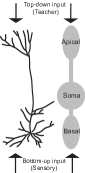
Figure 1: Depiction of a pyramidal cortical neuron (left) and its multi-compartment model used in artificial neural networks (right). Adapted from [6].

Since providing a top-down error signal has been very successful in deep learning[7, 8], some neuromorphic implementations have recently focused on using errors for online learning [9, 10]. Moreover, many neuroscientific studies have recently focused on error-based learning in the brain [11, 12]. In these studies, an error at the output units is assessed by comparing the self-generated activity of the neurons with a target activity. This error is then sent to the neurons as a feedback signal. Neurons are modeled with multiple compartments with several active dendritic branches, each directly linked to a somatic compartment (Fig. 1). The feedback signals arrive on the distal Apical dendrites, while proximal Basal dendrites receive feed-forward sensory information. Such types of models have been shown to implement error-backpropagation using biologically-plausible plasticity mechanisms [11, 12, 6].

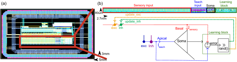
Figure 2: (a) A layout-view of the 3x5 $mm^{2}$ design. The circuits proposed are highlighted in the image and are composed of 4 individual neurons. (b) A close-up of a single neuron. The dendritic branches, the soma, and the learning block are all highlighted both in the schematic view and in the physical layout. The Sensory input is made up of 40 excitatory and 16 inhibitory plastic synapses. The Teach input is made up of 3 excitatory and 5 inhibitory non-plastic synapses.

Inspired by these studies, we developed mixed-signal electronic circuits that implement power-efficient online plasticity mechanisms that can be interfaced to neuromorphic synapse and neuron circuits. Specifically, since the synaptic weight precision is limited by the area of the memory that can be implemented on-chip, an interface circuitry is required to translate the analog weight updates to these low-bit precision memories. To solve this, we implement stochastic rounding on chip, which converts the analog weight updates to a probability of synaptic weight change  [13, 14]. Additionally, this mechanism provides robustness to the weight update process by reducing the probability of updates as the error decreases to near-zero values.

We describe the software-hardware co-design approach that validated the circuit designs with behavioral simulations, and that led to the fabrication of the circuits using a standard 180 nm Complementary Metal-Oxide-Semiconductor (CMOS) process (Fig. 2). In the next sections we present the learning algorithm, the circuits implementations, and finally, the results from the hardware and software simulations.

II The algorithm

II-A The multi-compartment neuron model

The selected neuron model used is a multi-compartment Leaky Integrate and Fire (LIF) neuron in which currents from two dendritic branches, the bottom-up Sensory branch ($I_{Sensory}$) and the top-down Teacher branch ($I_{Teach}$), get integrated into a somatic compartment ($I_{Soma}$). This is summarized in Eq. 1.

$$\tau_{Soma}\cfrac{dI_{Soma}}{dt}+I_{Soma}(t)={{I_{Sensory}(t)}+{I_{Teach}(t)}}$$ (1)

where $\tau_{Soma}$ is the neuron’s time constant.

The Sensory and Teach dendritric dynamics are modeled by Eq.  2 and 3 respectively.

$$\tau_{Sensory}\cfrac{d{I_{Sensory_{j}}}}{dt}+{I_{Sensory_{j}}}=\sum\limits_{i}\sum\limits_{n}{I_{w_{ij}}}\delta_{i,s}(t-t_{n})$$ (2)

$$\tau_{Teach}\cfrac{d{I_{Teach_{j}}}}{dt}+{I_{Teach_{j}}}=\sum\limits_{n}{I_{w_{Teach}}}\delta_{i,t}(t-t_{n})$$ (3)

where $i,j$ represents the input and output neurons respectively, and $n$ is the time at which the input neurons spike. The $\delta_{i,s}$ and $\delta_{i,t}$ function describes the input spike trains at the Sensory and Teach branches, respectively. $\tau_{Sensory}$ and $\tau_{Teach}$ represent the respective Sensory and Teach dendritic time constants, $I_{w_{ij}}$ is the plastic synaptic strength between Sensory input $i$ and output neuron $j$ (Basal input), and ${I_{w_{Teach}}}$ is the non-plastic constant teacher current (Apical input).

II-B The learning rule

The learning rule follows a dendritic-based prediction learning [15] which resembles Delta rule. The Delta rule is the simplest form of gradient-descent learning, minimizing a single-layer neural network’s Least Mean Square (LMS) error. Here, the error is defined as the difference between the Sensory and Teach dendritic branches as is described in Eq. 4.

$${err_{ij}}=\alpha({I_{Teach_{j}}}-{I_{Sensory_{j}}})x_{i}|I_{Teach_{j}}|$$ (4)

where $\alpha$ is the learning rate and the error is calculated every time a pre-synaptic spike occurs ($x_{i}$). This error is scaled by the absolute value of$(I_{Teach_{j}}$, which is in case of a true targets, is positive and negative otherwise. In this way if the teaching signal is not present (i.e., $I_{Teach_{j}}=0$) the learning will stop.

To manage the changes on the limited-bit precision synaptic memory (here 4 bits) with the analog weight updates, that are proportional to the error signal, we employed a stochastic rounding mechanism [13, 14, 16]. This is implemented by comparing the magnitude of the error to a random number (here 6 bits), and if greater, incrementing or decrementing the weight depending on the sign of the error. Otherwise, no weights are updated. Therefore, the probability of weight update is proportional to the error in the network. This is summarized in Eq. 5.

$$\Delta w_{ij}(@x_{i})=\begin{cases}\pm 1\quad\text{if}\quad|err_{ij}|>rand()\\ 0\quad\text{otherwise}\end{cases}$$ (5)

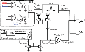
Figure 3: Block diagram of the online learning mechanism. It consists of error generation and stochastic rounding.

III The neuromorphic system

III-A The network architecture

The circuits have been fabricated in a prototype chip using a 180 nm CMOS technology. The network occupies an area of $15mm^{2}$ ($5\,mm$ x $3mm$). The total area occupied by the neural core presented here is $1.01mm^{2}$. The physical layout of the network is shown in Fig. 2a.
The neural core can be broken down into four identical rows, where each row has one neuron and 64 plastic and non-plastic synapses (Fig. 2b). The total synaptic activity consists of two main dendritic branches. The Sensory branch (Basal, ${I_{Sensory}}$) has 56 independent excitatory and inhibitory plastic synapses (4 bit resolution), while the Teach branch (Apical, ${I_{Teach}}$), has 8 excitatory and inhibitory non-plastic synapses. The excitatory synapses inject a positive current into the dendrite, while the inhibitory ones takes current away from it. Therefore, the total current in both dendritic branches is the subtraction between the excitatory and inhibitory currents.

Upon the arrival of any input event on the Sensory dendritic branch, the Soma integrates the weighted input, and if it reaches a threshold, it generates an output spike. Moreover, the Sensory input event activates the learning block which computes the error, generates a random number, and sends update signals if the former is greater than the latter.

III-B The learning circuits

Figure 3 illustrates the block diagram of the learning mechanism, which consists of the error-generation and stochastic rounding blocks.

III-B1 Error generation

The error generation implements Eq. 4, getting ${I_{Teach}}$ and ${I_{Sensory}}$ as inputs. The magnitude and the direction of weight update are determined by the absolute value ($abs$), and Winner-Takes-All (WTA) circuit, respectively.

The $abs$ circuit calculates the error by subtracting ${I_{Teach}}$ and ${I_{Sensory}}$ from each other in two directions, using $G_{1}$ and $G_{2}$ transconductance amplifiers, giving rise to the positive (${V_{PosErr}}$) and negative (${V_{NegErr}}$) errors. Depending on which input is greater, either the $M_{1}$ or the $M_{2}$ transistor is on, whose current flows in $I_{AbsErr}$ giving rise to the absolute value of the error [17]. The $abs$ circuit is biased with ${I_{Teach}}$ to gate the generation of the error signals only when the teacher is presented. If the teacher is not present (${I_{Teach}}$ = 0), the $abs$ circuit is OFF. The Teach input can be either positive or negative, however the $abs$ circuit is biased always with the unsigned ${I_{Teach}}$. The learning block is designed to distinguish between a positive and a negative Teach input and change the synaptic weights accordingly.

The WTA decides the direction of update ($UP$ or $DOWN$) depending on which one of ${V_{PosErr}}$ and ${V_{NegErr}}$ is higher [18]. If ${V_{PosErr}}$ and ${V_{NegErr}}$ are equal, $UP$ and $DOWN$ output of the WTA circuit are both set to low, and thus no update signal is generated. This makes the learning more robust by avoiding unnecessary updates as the system is reaching its optimal output.

III-B2 Stochastic rounding circuits

The stochastic rounding block implements Eq. 5. Every time a pre-synaptic spike is generated, a 6-bit pseudo-random number is generated from an on-chip Linear Feedback Shift Register (LFSR) and is converted into an analog current (${I_{random}}$) using a 6-bit current Digital to Analog Converter (DAC). The ${I_{random}}$ current is then compared to the error current, $I_{absolute}$, generated by the error generation block (see III-B1). The comparison happens through a modified version of Traff’s current comparator (CC) proposed in [19]. Traff’s comparator input voltage is determined by the difference between ${I_{absolute}}$ and ${I_{random}}$ and is initially around ${Vdd/2}$. As soon as ${I_{absolute}}$ and ${I_{random}}$ are not equal, the input voltage increases or decreases and the change is amplified by the CC. The output ${OktoUpdate}$ is set to high/low if $I_{absolute}$ is larger/less than $I_{random}$. The ${OktoUpdate}$ signal allows the weight update signals ($UP$ and $DOWN$) to pass through, only when it is high.

Since the probability of generating ${OktoUpdate}$ is proportional to the error, as the error is reduced, the probability of generating an update is also reduced. This leads to less weight updates as the system is reaching the optimal output which makes the learning more robust and power efficient.

It is worth noting that the event-driven nature of the input allows us to use a single stochastic rounding block for the entire row and generate an update signal on the arrival of any pre-synaptic sensory input events.

IV Results

IV-A Circuit simulations

To validate the learning rule at a schematic-level, we show the simulation results from one of the four identical rows of the chip (Figure 4). Initially, a positive teacher (dotted blue in Fig. 4a) is presented, which causes the weights of the excitatory synapses (dashdotted in orange in Fig. 4a) to strengthen and minimize the error between the teacher and the sensory branch (shown in red in Fig. 4a). At t = 0.3s, a negative teacher is shown to the network, which causes the strengthened excitatory synapses to weaken, and the inhibitory synapses (dashdotted in green in Fig. 4b) to strengthen and minimize the error between the two dendritic branches.

Table I shows a direct comparison with previous works using on-chip on-line error-based learning [16, 20]. The area in  [16] has been normalized to a 180 nm technology node to allow for a better comparison with our work. The energy per update in  [20] is not directly comparable to our work, since the weight update is calculated in a microcontroller, and the reported figure does not take that into account. The 720 pJ reported in this work, is the total energy in one row consumed to calculate and update one bit of synaptic memory.

Feature	[16]	[20]	This work
Resources	C5×5@10	Re-configurable	4 neurons
or topology	–FC128–FC10		64 synapse
Implementation	Digital	Digital	Mixed-signal
Learning	on-line	on-line	on-line
	error-based	re-configurable	error-based
Synaptic
resolution	8-bit	1-9 bits	4-bit
Static power	61$\mu{W}$	not-applicable	455 nW
consumption			per neuron
Energy metric	N/A	120  pJ	720 pJ
		per weight update	per weight update
Technology node	28 nm FDSOI	14  nm FinFET	180 nm CMOS
Power supply	0.6 V	0.75 V	1.8 V
Area	$13.2\,mm^{2}$	not-applicable	$15\,mm^{2}$

[1]The learning block is implemented using a micro controller: area and power figures are not directly comparable.
[2]Design normalized to a 180 nm technology node.

TABLE I: Comparison with previous works using on-chip on-line error-based learning.

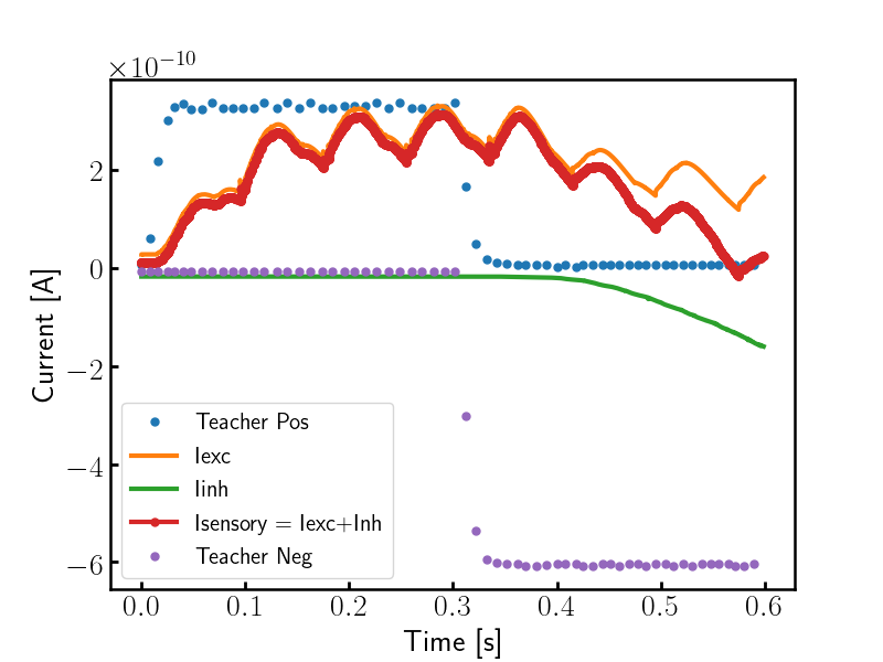
(a)

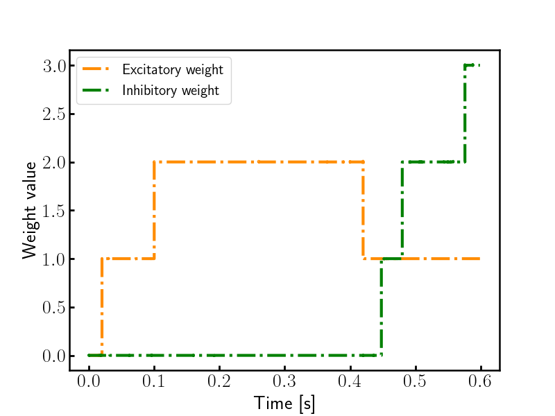
(b)

Figure 4: Cadence simulations of the learning signals of a single neuron; (a) example of the signals involved in the learning process. The sensory dendritic current (in red) is the sum of the excitatory (in orange) and inhibitory currents (in green). A positive teacher signal (dotted in blue) is presented until t = 0.3s. A negative teacher signal (dotted in purple) is presented after that. (b) weight changes associated with the learning of (a). The weights change their value to minimize the error between the sensory current and the teacher current. An excitatory (dashdotted in orange) and an inhibitory (dashdotted in green) weight are shown.

IV-B System

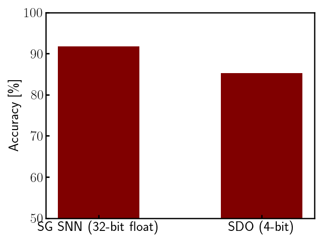
(a)

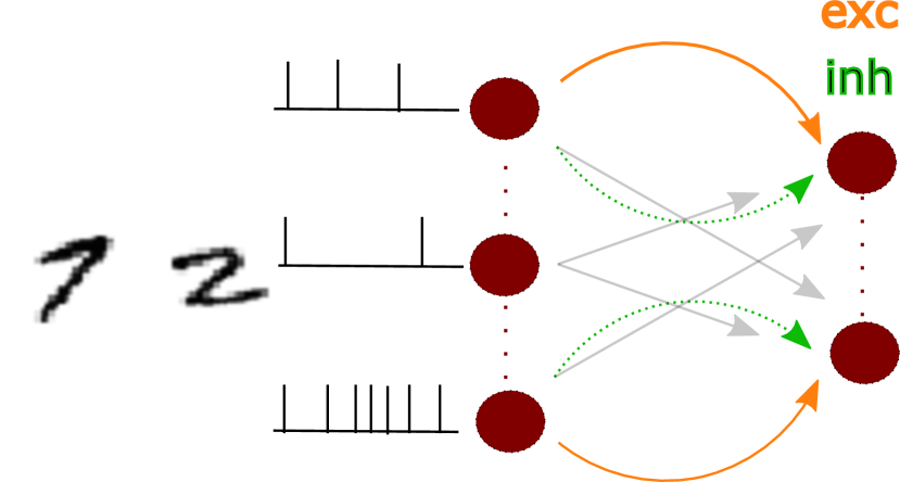
(b)

Figure 5: MNIST benchmarking results. (a) Accuracy comparison of a 784-10 SNN network trained using surrogate gradients (SG) versus the same network trained using the proposed stochastic dendritic online (SDO) rule. 80-20 randomized division was used between training and testing. (b) Topology of the network in the SDO simulations: input pixels are connected to the output layer with excitatory (in orange) and inhibitory (in green) connections.

The proposed learning rule and system were fully modeled using the BRIAN2 simulator [21]. Fig. 5 shows the results of a shallow network (with topology 784-10 neurons) on the MNIST handwritten digit dataset. It shows a direct comparison with a Spiking Neural Network (SNN) trained with surrogate gradient descent [22] using 32-bit floating point (SG SNN), while the proposed implementation uses 4-bit weights. The SG SNN reaches 91% accuracy while the stochastic dendritic online implementation reaches above 85%. Interestingly [23] achieves similar results with the same network topology.

Although both are SNNs, the difference in performance can be attributed to that (i) the hardware network implements weight updates on streaming data, with a batch size of one, compared to a batch size of 256 in SG SNN, and (ii) the hardware uses only 4 bits of precision compared to the floating point resolution in the SG SNN case.

V Discussion and Conclusion

We presented a prototype neuromorphic chip designed and fabricated in 180 nm technology which implements stochastic dendritic-based online learning. We proposed an algorithm–circuits co-design approach and validated it with circuit simulations that demonstrate the proper operation of the learning rule.

We benchmarked our system via system-level simulations, and obtained above 85% accuracy on the MNIST dataset using only a one-layer network with 4-bit weight precision.

As our circuits show that single neurons can adapt based on their incoming activity, they represent a valid candidate for adaptive “edge computing” applications that require online learning. To this end, future work will include interfacing the chip with signals that need to be classified at the edge, such as biomedical or industrial signals.

References

- [1] G. Indiveri and S.-C. Liu. Memory and information processing in neuromorphic systems. Proceedings of the IEEE, 103(8):1379–1397, 2015.
- [2] Abu Sebastian, Manuel Le Gallo, Riduan Khaddam-Aljameh, and Evangelos Eleftheriou. Memory devices and applications for in-memory computing. Nature nanotechnology, 15(7):529–544, 2020.
- [3] Arianna Rubino, Can Livanelioglu, Ning Qiao, Melika Payvand, and Giacomo Indiveri. Ultra-low-power FDSOI neural circuits for extreme-edge neuromorphic intelligence. IEEE Transactions on Circuits and Systems I: Regular Papers, 68(1):45–56, 2020.
- [4] Giacomo Indiveri and Yulia Sandamirskaya. The importance of space and time for signal processing in neuromorphic agents. IEEE Signal Processing Magazine, 36(6):16–28, 2019.
- [5] Chetan Singh Thakur, Jamal Lottier Molin, Gert Cauwenberghs, Giacomo Indiveri, Kundan Kumar, Ning Qiao, Johannes Schemmel, Runchun Wang, Elisabetta Chicca, Jennifer Olson Hasler, Jae-sun Seo, Shimeng Yu, Yu Cao, André van Schaik, and Ralph Etienne-Cummings. Large-scale neuromorphic spiking array processors: A quest to mimic the brain. Frontiers in Neuroscience, 12:891, 2018.
- [6] Jordan Guerguiev, Timothy P Lillicrap, and Blake A Richards. Towards deep learning with segregated dendrites. Elife, 6:e22901, 2017.
- [7] Brian Crafton, Abhinav Parihar, Evan Gebhardt, and Arijit Raychowdhury. Direct feedback alignment with sparse connections for local learning. arXiv, pages 1–13, 2019.
- [8] Friedemann Zenke and Emre O Neftci. Brain-Inspired Learning on Neuromorphic Substrates. Proceedings of the IEEE, pages 1–16, 2021.
- [9] Melika Payvand, Mohammed E. Fouda, Fadi Kurdahi, Ahmed M. Eltawil, and Emre O. Neftci. On-Chip Error-Triggered Learning of Multi-Layer Memristive Spiking Neural Networks. IEEE Journal on Emerging and Selected Topics in Circuits and Systems, 10(4):522–535, 2020.
- [10] Matteo Cartiglia, Germain Haessig, and Giacomo Indiveri. An error-propagation spiking neural network compatible with neuromorphic processors. In 2nd IEEE International Conference on Artificial Intelligence Circuits and Systems (AICAS), pages 84–88. IEEE, 2020.
- [11] João Sacramento, Rui Ponte Costa, Yoshua Bengio, and Walter Senn. Dendritic cortical microcircuits approximate the backpropagation algorithm. In Advances in Neural Information Processing Systems, pages 8721–8732, 2018.
- [12] James CR Whittington and Rafal Bogacz. An approximation of the error backpropagation algorithm in a predictive coding network with local hebbian synaptic plasticity. Neural computation, 29(5):1229–1262, 2017.
- [13] Lorenz K Muller and Giacomo Indiveri. Rounding methods for neural networks with low resolution synaptic weights. arXiv preprint arXiv:1504.05767, 2015.
- [14] Matthieu Courbariaux, Yoshua Bengio, and Jean-Pierre David. Binaryconnect: Training deep neural networks with binary weights during propagations. In Advances in neural information processing systems, pages 3123–3131, 2015.
- [15] Robert Urbanczik and Walter Senn. Learning by the dendritic prediction of somatic spiking. Neuron, 81(3):521–528, 2014.
- [16] Charlotte Frenkel, Jean-Didier Legat, and David Bol. A 28-nm convolutional neuromorphic processor enabling online learning with spike-based retinas. In 2020 IEEE International Symposium on Circuits and Systems (ISCAS), pages 1–5. IEEE, 2020.
- [17] Melika Payvand, Manu V Nair, Lorenz K Müller, and Giacomo Indiveri. A neuromorphic systems approach to in-memory computing with non-ideal memristive devices: From mitigation to exploitation. Faraday Discussions, 213:487–510, 2019.
- [18] M. Payvand and G. Indiveri. Spike-based plasticity circuits for always-on on-line learning in neuromorphic systems. In IEEE International Symposium on Circuits and Systems (ISCAS), pages 1–5. IEEE, 2019.
- [19] H. Träff. Novel approach to high speed cmos current comparators. Electronics Letters, 28:310–311(1), January 1992.
- [20] Mike Davies, Narayan Srinivasa, Tsung-Han Lin, Gautham Chinya, Yongqiang Cao, Sri Harsha Choday, Georgios Dimou, Prasad Joshi, Nabil Imam, Shweta Jain, Yuyun Liao, Chit-Kwan Lin, Andrew Lines, Ruokun Liu, Deepak Mathaikutty, Steven McCoy, Arnab Paul, Jonathan Tse, Guruguhanathan Venkataramanan, Yi-Hsin Weng, Andreas Wild, Yoonseok Yang, and Hong Wang. Loihi: A neuromorphic manycore processor with on-chip learning. IEEE Micro, 38(1):82–99, 2018.
- [21] D. Goodman and R. Brette. Brian: a simulator for spiking neural networks in Python. Frontiers in Neuroinformatics, 2, 2008.
- [22] Emre O Neftci, Hesham Mostafa, and Friedemann Zenke. Surrogate gradient learning in spiking neural networks: Bringing the power of gradient-based optimization to spiking neural networks. IEEE Signal Processing Magazine, 36(6):51–63, 2019.
- [23] Charlotte Frenkel, Martin Lefebvre, Jean-Didier Legat, and David Bol. A 0.086-mm2 12.7-pj/SOP 64k-synapse 256-neuron online-learning digital spiking neuromorphic processor in 28-nm CMOS. IEEE Transactions on Biomedical Circuits and Systems, 13(1):145–158, 2019.