Combining Commonsense Reasoning and Knowledge Acquisition to Guide Deep Learning in Robotics

Abstract

Algorithms based on deep network models are being used for many pattern recognition and decision-making tasks in robotics and AI. Training these models requires a large labeled dataset and considerable computational resources, which are not readily available in many domains. Also, it is difficult to explore the internal representations and reasoning mechanisms of these models. As a step towards addressing the underlying knowledge representation, reasoning, and learning challenges, the architecture described in this paper draws inspiration from research in cognitive systems. As a motivating example, we consider an assistive robot trying to reduce clutter in any given scene by reasoning about the occlusion of objects and stability of object configurations in an image of the scene. In this context, our architecture incrementally learns and revises a grounding of the spatial relations between objects and uses this grounding to extract spatial information from input images. Non-monotonic logical reasoning with this information and incomplete commonsense domain knowledge is used to make decisions about stability and occlusion. For images that cannot be processed by such reasoning, regions relevant to the tasks at hand are automatically identified and used to train deep network models to make the desired decisions. Image regions used to train the deep networks are also used to incrementally acquire previously unknown state constraints that are merged with the existing knowledge for subsequent reasoning. Experimental evaluation performed using simulated and real-world images indicates that in comparison with baselines based just on deep networks, our architecture improves reliability of decision making and reduces the effort involved in training data-driven deep network models.

1 Introduction

Imagine an assistive robot that has to clear away toys and objects that children have (mis)placed in different configurations in different rooms of a home. Figure 1 shows an example simulated scene of toys in a room. The robot’s task poses knowledge representation, reasoning, and learning challenges because it is difficult to provide labeled training examples of all possible arrangements of objects or of all combinations of object attributes. Also, the robot has to reason with different descriptions of incomplete domain knowledge and the associated uncertainty. This may include qualitative descriptions of commonsense knowledge about the domain objects, e.g., default statements such as “structures with a large object placed on a small object are typically unstable” that hold in all but a few exceptional circumstances, and an initial grounding of the relations between objects, e.g., meaning in the physical world for “left of” and “behind”. The robot may also obtain quantitative descriptions of knowledge and uncertainty, e.g., from algorithms for sensing and navigation that provide information such as “I am 90% certain the big red box is stable”. Furthermore, human participants are unlikely to have the time and expertise to interpret raw sensor data or to provide comprehensive feedback, and the robots’ decisions may be incorrect or sub-optimal if they are based on incomplete or incorrect domain knowledge.

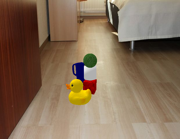
Figure 1: A simulated scene with toys on the ground. The robot has to reason about occlusion of objects and stability of object configurations to reduce clutter.

We use the robot assistant (RA) domain described above as a motivating example to describe the capabilities of an architecture that is a step towards addressing the underlying knowledge representation, reasoning, and learning challenges. In particular, we consider the scene understanding tasks of estimating the partial occlusion of objects and the stability of object configurations. State of the art methods for such tasks are based on deep network architectures. Although these methods often provide high accuracy, they require a large number of labeled training examples, are computationally expensive, and make it difficult to understand the decisions made. Research in cognitive systems has demonstrated the benefits of considering different representations and reasoning methods, and of coupling representation, reasoning, and learning such that they inform and guide each other. Drawing inspiration from such systems, our architecture exploits the complementary strengths of non-monotonic logical reasoning based on incomplete commonsense domain knowledge, deep learning, and incremental inductive learning of constraints governing domain states.

In the context of the RA domain, a robot equipped with our architecture obtains 3D point clouds of the scenes of interest. The robot is also provided incomplete domain knowledge in the form of the type and attributes (e.g., color, size) of some domain objects; an initial qualitative grounding (i.e., meaning in the physical world) of prepositional words (e.g., “above”, “left_of”, and “near”) describing spatial relations between objects in the scene; and some axioms (i.e., rules) governing actions, states, and change in the domain, including default statements such as “any object configuration with a large object placed on a small object is typically unstable” that is true in all but a few exceptional circumstances. The architecture enables the robot to:

1. Interactively and cumulatively learn and revise a quantitative (i.e., metric) grounding of the spatial relations between objects, using the qualitative grounding, point cloud data of objects in a small number of input (RGB-D) images, and limited feedback from humans.

2. Use non-monotonic logical reasoning to perform the estimation tasks on any given input image using a relational representation of the information extracted from the image (e.g., object attributes, spatial relations between objects) and the incomplete (prior) domain knowledge.

3. Automatically identify regions of interest (ROIs) in images for which the estimation tasks cannot be completed using non-monotonic logical reasoning. These ROIs and the corresponding (occlusion, stability) labels are used to guide the construction of deep networks during training, and the ROIs are processed by the trained networks during testing, for the estimation tasks.

4. Incrementally learn previously unknown relational constraints using the information used to train the deep networks, i.e., the relational information extracted from the ROIs and the corresponding labels. A heuristic approach inspired by human forgetting helps merge and update the learned and existing knowledge for subsequent reasoning.

We use CR-Prolog, an extension of Answer Set Prolog (ASP) [4, 21], for non-monotonic logical reasoning with incomplete commonsense domain knowledge. We also adapt existing network architectures for the deep learning component of our architecture. The design and evaluation of our architecture is subject to two caveats:

• State of the art scene understanding methods often focus on generalizing across different tasks and domains using a large number of labeled training examples. Our focus, on the other hand, is on enabling a robot to use a small number of images and to automatically limit learning to previously unknown information relevant to the tasks at hand in any given domain. We thus do not use existing benchmark datasets for experimental comparison. Instead, we use a small set of real world and simulated images of scenes in the robot assistant domain described above.

• Given our focus on exploring the interplay between representation, reasoning, and learning, we do not compare our architecture’s performance against existing methods for just the reasoning or learning components. Instead, we run ablation studies and compare against data-driven baselines that use deep networks to perform the estimation tasks of interest. For ease of understanding, we also limit perceptual processing to that of 3D point clouds of scenes, and limit previously unknown domain knowledge to state constraints. We have explored the learning of other types of axioms, and the use of these axioms to interpret the behavior of deep networks, in other work [42, 55].

Some components of this architecture have been described in conference papers, e.g., the incremental learning of a quantitative grounding of spatial relations [38] and the incremental learning of state constraints [39, 49]. Here, we describe these components in detail, highlight recent revisions to these components, and explore the capabilities supported by the interplay between these components. We also provide additional experimental results to demonstrate a marked increase in the accuracy of decision-making and a reduction in the computational effort in comparison with architectures that only use deep networks.

The remainder of this paper is organized as follows. First, Section 2 discusses related work to motivate our architecture, whose components are described in Section 3. The experimental setup and results are described in Section 4. Finally, the conclusions and directions for further research are discussed in Section 5.

2 Related Work

The scene understanding tasks in the motivating RA domain considered in this paper are representative of a wide range of estimation and prediction problems that pose the knowledge representation, reasoning, and learning problems of interest. Deep networks provide state of the art performance for these problems and for many other computer vision and control problems. For instance, a Convolutional Neural Network (CNN) has been used to predict the stability of a tower of blocks [34, 35], the movement of an object sliding down an inclined surface and colliding with another object [61], and the trajectory of an object after bouncing against a surface [47]. However, CNNs and other deep networks require a large number of labeled examples and considerable computational resources to learn the mapping from inputs to outputs. In addition, it is difficult to understand the operation of the learned networks, which also makes it challenging to transfer knowledge learned in one scenario or task to a related scenario or task [57, 66].

Since labeled training examples are not readily available in many domains, researchers have explored approaches that simulate labeled data or use prior knowledge to constrain learning. For instance, physics engines have been used to generate labeled data for training deep networks that predict the movement of objects in response to external forces [17, 43, 60], or for understanding the physics of scenes [5]. A recurrent neural network (RNN) architecture augmented by arithmetic and logical operations has been used to answer questions about scenes [44], but it used textual information instead of the more informative visual data and did not support reasoning with commonsense knowledge. Another example is the use of prior knowledge to encode state constraints in the CNN loss function; this reduces the effort in labeling training images, but it requires the constraints to be encoded manually as loss functions for each task [56]. The structure of deep networks has also been used to constrain learning, e.g., by using relational frameworks for visual question answering (VQA) that consider pairs of objects and related questions to learn the relations between objects [51]. This approach, however, only makes limited use of the available knowledge, and does not revise the constraints over time.

For many problems in robotics and AI, prior domain knowledge often includes the grounding, i.e., an interpretation in the physical world, of words such as in, behind, and above representing spatial relations between objects. Many systems for grounding such relations are based on manually encoded descriptions, or on learning algorithms. Methods using the former typically rely on Qualitative Spatial Representations (QSR) of spatial relations [12, 62, 65], whereas in the latter case, it is more common to use Metric Spatial Representations (MSR), i.e., measures based on distances and angles [6, 37]. QSR-based approaches often approximate objects as points and establish static boundaries between spatial relations, whereas the grounding of spatial relations is likely to change over time in dynamic domains. MSR-based systems often learn the grounding of spatial relations offline or in a separate training phase. Specific instances of QSR and MSR have been used for different tasks in robotics and computer vision, e.g., QSR relations have been extracted from videos [19], MSR and kd-trees have been used to infer spatial relations between objects [67], QSR and MSR have been compared for scene understanding on robots [58], the relative position of objects has been used to predict successful action execution [16], and methods have been developed to reason about and learn spatial relations between objects [26, 28]. Specialized meetings have explored the use of natural language to describe spatial relationships between objects [11, 59]. Deep networks have also been used to infer spatial relations between objects using images and natural language expressions, for manipulation [45], navigation [46], and human-robot interaction [52]. Our approach for learning the grounding of spatial relations starts with a manually-encoded generic (QSR) grounding, and interactively learns a specialized (MSR) grounding from experience and human feedback [38].

There is an established literature on generic methods for learning domain knowledge. Examples include the incremental revision of a first-order logic representation of action operators [22], the use of inductive logic programming to learn domain knowledge represented as an Answer Set Prolog (ASP) program [31, 32], and work in our group on coupling of non-monotonic logical reasoning, inductive learning, and relational reinforcement learning to incrementally acquire actions and axioms [55]. Our approach for learning domain axioms is inspired by work in interactive task learning, a general framework for acquiring domain knowledge using labeled examples or reinforcement signals obtained from domain observations, demonstrations, or human instructions [9, 30]. However, unlike approaches that learn from many training examples, our approach seeks to incrementally acquire and revise domain knowledge from limited, partially-defined, training examples. It can be viewed as building on early work on heuristic search through the space of hypotheses and observations [53], but such methods have rarely been explored for scene understanding.

Studies in neural-symbolic learning and reasoning have explored the benefits and limitations of interleaving statistical learning and symbolic reasoning [7, 50]. For example, the probabilistic logic programming language ProbLog has been extended to DeepProbLog, which supports symbolic and sub-symbolic inference, program induction, and deep (neural) learning from examples based on neural predicates [36]. Another example is a neural-symbolic visual question answering system that uses deep networks to infer structural object-based scene representation from images, and to generate a hierarchical (symbolic) program of functional modules from the question. Running the program on the representation answers the desired question [64]. Many of these methods rely on classical first-order logic [25] that is not expressive enough for reasoning with commonsense knowledge, use simplified neural architectures corresponding to specific symbolic representations [18], associate probability values with all logic statements which is not always meaningful, or do not clearly establish the link between reasoning and learning. In addition, although retracting imperfect or incorrect beliefs has long been considered as important as learning new knowledge [10, 24], existing neural-symbolic approaches rarely support the automatic detection and correction of errors in learned knowledge. In parallel, there has been much work on interpreting the operation of deep networks, e.g., by computing gradients and decompositions at different layers of the network, and providing heatmaps that indicate the features most relevant to the observed output(s) of deep network [2, 50]. However, these approaches do not exploit the incomplete commonsense domain knowledge for reliable and efficient reasoning and learning, and for generating explanations in the form of relational descriptions.

A recent evaluation of state of the art computational models for reasoning (and understanding) on a diagnostic video dataset revealed that existing methods are able to answer descriptive questions about the scene, but perform poorly on explanatory, predictive, and counterfactual questions [63]. The results indicate that causal reasoning methods need an understanding of the domain dynamics and causal relations. This understanding can be provided using models of domain physics, as described above. Work in our research group, on the other hand, is inspired by research in cognitive systems, which indicates that coupling knowledge representation, reasoning, and interactive learning, can help address the limitations described above [23, 42, 49, 55, 54]. The architecture described in this paper combines the complementary strengths of deep learning, reasoning with incomplete commonsense knowledge, and inductive learning. It explores the interplay between our prior work on incrementally learning a grounding of spatial relations between objects [38] and on learning constraints that govern domain states [39, 49], introduces a heuristic approach inspired by human forgetting [13] to detect and correct errors while merging the learned knowledge with existing knowledge, and describes detailed results of ablation studies and other experiments evaluating the capabilities of our architecture.

3 Reasoning and Learning Architecture

Figure 2 is an overview of our reasoning and learning architecture whose components are adapted and described in this paper in the context of estimating the occlusion of objects and stability of object configurations in the RA domain. An object is considered to be occluded if the view of any minimal fraction of its frontal face is hidden by another object, and a configuration (or structure), i.e., a stack of objects, is unstable if any object in the structure is unstable. This architecture takes as input RGB-D images of scenes with different object configurations. During training, the inputs also include the occlusion labels of objects and the stability labels of object configurations in these images. Also, a static qualitative representation is provided for the grounding of the prepositional words encoding spatial relations between objects; this grounding is used to learn and revise a histogram-based metric representation of the grounding.

For any given image, our architecture first attempts to assign the desired (occlusion and stability) labels to scene objects using ASP-based non-monotonic logical reasoning. This reasoning considers the incomplete commonsense domain knowledge and the relational (i.e., logic-based) representation of the noisy information extracted from the RGB-D image, i.e., object attributes and spatial relations between objects. If such reasoning is able to complete the estimation tasks, i.e., provide correct labels during training and estimate labels during testing, no further analysis of this image is performed. Otherwise, an “attention mechanism” reasons with existing knowledge (of task and domain) to automatically identify Regions of Interest (ROIs) in the image relevant to the tasks to be performed, with each ROI containing one or more objects. A CNN is trained with image ROIs and the corresponding ground truth labels, and used (during testing) to map these ROIs to the desired labels. In addition, ROIs used to train the CNN are also used as input to a decision tree induction algorithm that maps object attributes and spatial relations to the target labels. Branches in the tree that have sufficient support among the training examples are used to construct axioms representing state constraints. The learned constraints are automatically and heuristically merged with the existing domain knowledge by adding or removing axioms as appropriate, and used for subsequent reasoning. We will use the following illustrative domain to describe the components of our architecture in more detail.

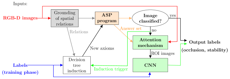
Figure 2: Architecture combines the complementary strengths of deep learning, non-monotonic logical reasoning with incomplete commonsense domain knowledge, and decision tree induction; architecture illustrated here in the context of estimating occlusion of objects and stability of object structures.

Example 1

[Robot Assistant (RA) Domain]
A simulated robot analyzes images of scenes containing objects in different configurations. The goal is to estimate occlusion of objects and stability of object structures, and to rearrange object structures so as to minimize clutter. Domain knowledge includes incomplete information about the object’s attributes such as $size$ (small, medium, large), $surface$ (flat, irregular), and $shape$ (cube, cylinder, duck), and the spatial (i.e., geometric) $relation$ between objects (above, below, front, behind, right, left, close). The robot can move objects to achieve the desired goals. Domain knowledge also includes some axioms governing domain dynamics (i.e., states and actions) but some other axioms may be unknown, e.g.:

• Placing an object on top of an object with an irregular surface causes instability;

• An object is not occluded if all objects in front of it are moved away.

In addition to learning the previously unknown axioms, the existing axioms may also need to be revised over time based on observations, e.g., the robot may find that it is possible to place an object on another with an irregular surface under certain conditions.

Using this domain as a running example, Section 3.1 first describes the approach for incremental and interactive grounding of the spatial relations between objects. Section 3.2 describes the approach for representing and reasoning with incomplete commonsense domain knowledge and the information extracted from images to assign the desired labels. Next, Section 3.3 describes the identification of the relevant ROIs in images for which ASP-based reasoning could not assign (correct) labels, and the learning of CNNs that map features from these ROIs to the desired labels. Finally, Section 3.4 describes the incremental decision-tree induction of previously unknown domain axioms, and the heuristic approach to merge and revise the new axioms and existing knowledge.

3.1 Grounding of Spatial Relations

Our architecture includes a hybrid approach, which combines a Qualitative Spatial Representation (QSR) and a Metric Spatial Representation (MSR), for grounding (i.e., assigning meaning in the physical world for) the prepositional words encoding the spatial relations between scene objects. Figure 3 presents an overview of our approach. We consider seven position-based prepositions (in, above, below, front, behind, right, left) and three distance-based prepositions (touching, not-touching, far). These prepositions are used to encode spatial relations between specific scene objects as logic statements in an ASP program. The QSR module provides an initial, manually-encoded, generic grounding of spatial relations, which is used to extract spatial relations between pairs of 3D point clouds in any given input scene. Human feedback, when available, is in the form of labels for the spatial relations between pair(s) of point clouds in a scene. Both the QSR-based output and human feedback are transmitted by the control node to the MSR module, which incrementally acquires and revises a histogram-based grounding of the prepositions for spatial relations. Assuming human feedback to be accurate, the control node also computes the relative trust in the two groundings (QSR, MSR). The more reliable grounding is used to extract spatial relations between scene objects in subsequent images. This information is translated to logic statements that are added to the ASP program for inference. The individual modules of this approach are described below.

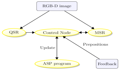
Figure 3: Overview of approach for grounding spatial relations between objects. A static QSR-based grounding and human input (if available) are used to incrementally learn and revise a MSR-based grounding.

3.1.1 Qualitative Spatial Representation

Our QSR model is based on an established approach described in [65]. For each 3D point cloud in any given image, a bounding box containing it (i.e., a convex cuboid around the object) is created—see Figure 4(a). If this point cloud is considered the reference object, the space around this object is divided into non-overlapping pyramids representing the relations left, right, front, behind, above and below—see Figure 4(b). In our implementation, the spatial relation of an object with respect to a reference object is determined by the non-overlapping pyramid around the reference that has most of the point cloud of the object under consideration. Also, any object with most of its point cloud located inside the bounding box of the reference object is said to be “in” the reference object. In this paper, we disregard the fact that this definition of in can lead to errors, especially in domains with non-convex objects, e.g., a book that is actually under a large table may be classified (incorrectly) as being in the table because the bounding box of the table envelopes most of the point cloud of the book.

(a)

(b)

Figure 4: QSR representation: (a) Bounding box for point cloud of a particular object; and (b) Pyramids delimiting space around the bounding box.

For ease of representation, our approach differs from [65] in the definition of the distance-related prepositions: touching, not-touching and far. For a pair of point cloud clusters, the $10\%$ closest distances between pairs of points drawn from the point clouds are computed, and the following heuristics are used to determine if the two objects are touching, not touching, or far (i.e., distinctly separated) from each other:

$$touching\ \Rightarrow\ distance(10\%)\ \leq\ 0.01$$ (1)

$$not\textnormal{-}touching\ \Rightarrow\ 0.01<distance(10\%)\ <1.0$$

$$far\ \Rightarrow\ distance(10\%)\ \geq\ 1.0$$

where distances are measured in meters. In other words, two objects are touching if the $10\%$ closest distances are less than or equal to $1cm$. The generic, manually-encoded grounding based on this QSR model does not change over time, whereas changes in factors such as camera pose may require the grounding to be revised. However, based on the reasonable assumption that the robot’s initial estimate of spatial relations is based on its view of the scene, our approach has the robot use the QSR-based grounding to identify spatial relations between objects in the initial stages. This grounding and human input of spatial relations between object pairs (when available) are used to incrementally learn and revise a specialized, quantitative grounding of spatial relations between objects, which we describe next.

3.1.2 Metric Spatial Representation

Unlike the QSR-based grounding, the MSR-based grounding model supports incremental and continuous updates from observations and human feedback. Assume temporarily that the MSR module receives a pair of point cloud clusters corresponding to two objects, and the prepositions of the spatial relations between the objects, e.g., from QSR or humans. Our MSR module grounds each preposition using histograms, also referred to as “visual words”, which are created by considering the point cloud data in a spherical coordinate system. Specifically, each point is represented by its distance to a reference point and two angles: $\theta\in[0\degree,180\degree]$ and $\varphi\in[-180\degree,180\degree]$. On a robot, the coordinate frame for grounding is defined with respect to the robot’s coordinate frame, its camera, and/or reference objects—information in one coordinate frame can be transformed to other coordinate frames as needed. Also, although processing the sensor input(s) can introduce noise, the non-monotonic logical reasoning and incremental learning abilities of our architecture support recovery from associated errors, as described later.

In our MSR-based representation, each of the seven position-based prepositions (in, left, right, front, behind, above, below) are ground using 2D histograms of angles $\theta$ and $\varphi$, whereas each of the three distance-based prepositions (touching, not-touching, far) are ground using 1D histograms of the $10\%$ closest distances between points in pairs of objects. Figures 5(a) and 5(b) show one illustrative example (each) of a histogram grounding a distance-based and position-based preposition. All histograms are normalized to ensure that large objects with many points do not have any undue influence on the grounding of relations.

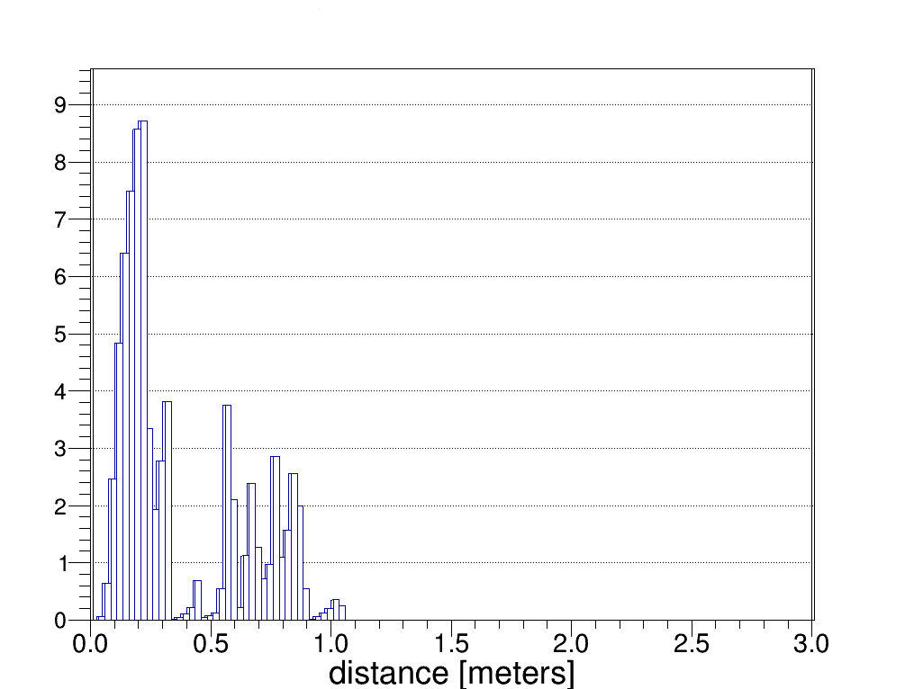
(a) 1D histogram for “not-touching”.

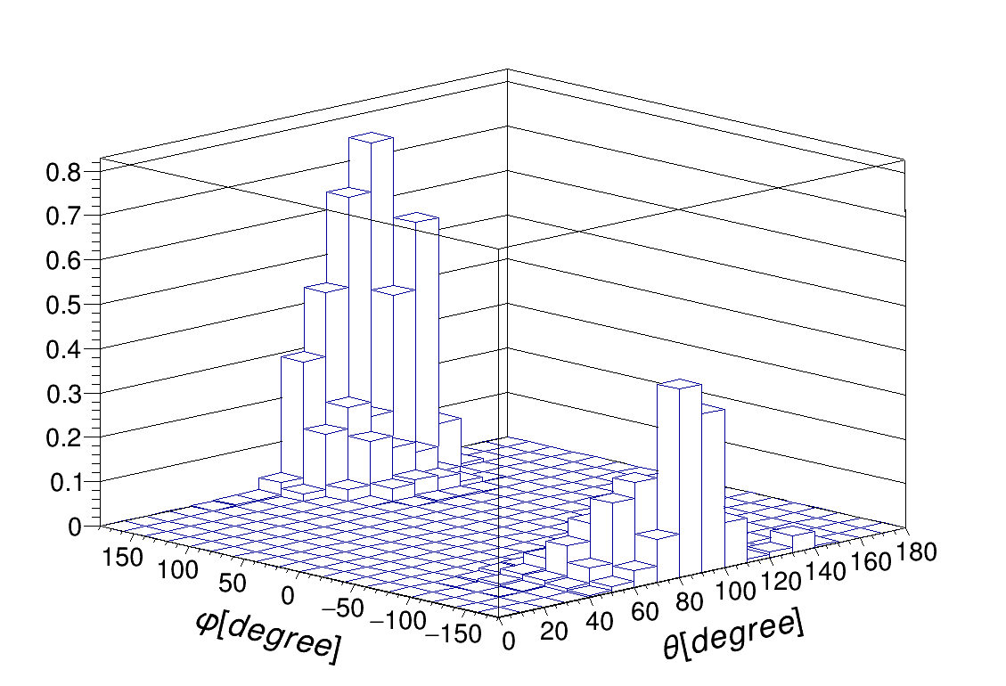
(b) 2D histogram for “left”.

Figure 5: Illustrative examples of MSR-based grounding: (a) 1D histogram grounding distance-based preposition “not-touching”; (b) 2D histogram grounding position-based preposition “left”.

Any learned MSR-based groundings are used for the subsequent new scenes. For any given pair of point cloud clusters in a new scene, the corresponding 2D and 1D histograms (i.e., visual words) are constructed. The learned visual words that are most similar to the extracted visual words are used to assign the distance-based and position-based spatial relations between the corresponding scene objects, e.g., “$object_{1}$ is below $object_{2}$ and not touching it”. These inferred spatial relations are automatically translated to logic statements that are added to the ASP program, e.g., $obj\_relation(below,~{}obj_{1},~{}obj_{2})$. Since axioms in the ASP program are applied recursively for inference, each point cloud cluster only needs to be considered once.

The similarity between visual words is computed using the standard intersection measure for 1D (distance) histograms. For computing the similarity between 2D (position) histograms, we use the $\chi^{2}$ measure, i.e., for two histograms $H$ and $G$:

$$D_{\chi^{2}}(H,G)=\sum\limits_{i}\dfrac{|h_{i}-g_{i}|^{2}}{2(h_{i}+g_{i})}$$ (2)

where $h_{i}$ and $g_{i}$ are bins in $H$ and $G$ respectively. Smaller values of this measure denote greater similarity. We only use this measure for 2D histograms because the boundaries between position-based relations are more difficult to define than those between distance-based relations. Once the spatial relations between a pair of point cloud clusters have been determined in a new scene, the learned visual words are updated using a standard normalized histogram merging approach, i.e., the MSR-based grounding is updated continuously. Next, we consider the use of human feedback when it is available.

3.1.3 Combined QSR-MSR Model

Recall that we are focusing on applications where many training examples and human supervision are not readily available. However, we do want to use the rich information encoded in human feedback when it is available. While the QSR-based grounding remains unchanged, the MSR-based grounding changes as new scenes are processed. Since the QSR-based and MSR-based groundings may disagree on the relation between some pairs of objects, the control node initially assigns high (low) confidence to the QSR-based (MSR-based) grounding. The relative confidence in each grounding is then updated based on the number of times the output from the grounding matches human input—the more reliable grounding is then used for processing the subsequent scenes. Note that this approach assumes that human input of spatial relations between point cloud clusters is accurate most of the time, i.e., each human participant providing feedback is expected to interpret spatial relations correctly. Incorrect human annotation can affect the confidence in a grounding and the subsequent grounding of spatial relations between objects, but our approach ensures that this only happens if the number of such incorrect annotations is comparable to the number of correct annotations.

Object shapes and sizes may also influence spatial relations depending on the viewpoint. However, since the MSR-based grounding is based on histograms of relative distances and angles, it can be used to infer spatial relations over a range of viewpoints. Also, the architecture has two mechanisms to limit and recover from errors. First, if the QSR-based grounding is applicable, e.g., viewpoint has not changed substantially from the initial view, the system can use it to obtain an initial estimate of spatial relations and incrementally acquire the MSR-based grounding. Second, if the QSR-based grounding is not applicable, it is still possible to acquire an MSR-based grounding from a small number of images and limited human input, and to use it for subsequent inference.

There are some caveats related to the proposed approach. First, the QSR-based grounding is assumed to be reasonably accurate initially. If this assumption does not hold and no human input is available, an inaccurate MSR-based grounding may be acquired, resulting in incorrect estimates of spatial relations. Also, it is possible to use an accurate MSR-based grounding or human input to revise the QSR-based grounding; we do not pursue that option in this paper in order to simplify the process of understanding the two different groundings. Second, human feedback improves the specialized MSR-based grounding and overall accuracy, but it is not essential for estimating spatial relations. Third, the encoded prepositions (with learned grounding) are translated to logic statements (i.e., observation literals) in an ASP program. These observations and the commonsense knowledge encoded in the ASP program limit possible relations between scene objects and help infer composite relations (e.g., on, close to, next to etc). For instance, the spatial relation $on$ may be defined by the following axiom:

$$obj\_relation(on,O_{1},O_{2})\ \leftarrow \ obj\_relation(above,O_{1},O_{2}),~{}obj\_relation(touching,O_{1},O_{2})$$ (3)

which states that if object $O_{1}$ is above $O_{2}$ and touching it, then $O_{1}$ is on $O_{2}$; the syntax and semantics of axioms are described in the next section. However, all axioms need not be defined in advance; our overall architecture supports reasoning with incomplete knowledge and incremental learning of these axioms as described later in this paper. Finally, we currently assume that each pair of objects is related through one position-based and one distance-based spatial relation, but not all the prepositions are (or need to be) mutually exclusive.

3.2 Knowledge Representation and Reasoning

This section describes our approach for representing and reasoning with incomplete domain knowledge. First, Section 3.2.1 introduces the action language used in our architecture. Next, Section 3.2.2 describes the use of the action language to represent a dynamic domain, and the translation of this domain representation to an ASP program for non-monotonic logical inference.

3.2.1 Action Language

Action languages are formal models of part of a natural language used for describing transition diagrams of dynamic domains. Our architecture uses the action language $\mathcal{AL}$ [20], which has a sorted signature with three types of sorts: statics, which are domain attributes whose values do not change over time; fluents, which are domain attributes that can be changed; and actions. Fluents can be inertial, which can be directly modified by actions and obey the laws of inertia, or defined, which are not directly changed by actions and do not obey inertia laws. A domain literal is a domain attribute p or its negation $\lnot$p. $\mathcal{AL}$ allows three types of statements:

$$\emph{l}~{}~{}\textbf{if}~{}~{}\emph{p}_{0},\ldots,\emph{p}_{m}~{}~{}~{}~{}~{}~{}~{}~{}$$ State Constraints

$$\emph{a}~{}~{}\textbf{causes}\ ~{}~{}\emph{l}_{in}~{}~{}\textbf{if}~{}~{}\emph{p}_{0},\ldots,\emph{p}_{m}~{}~{}~{}~{}~{}~{}~{}~{}$$ Causal Laws

$$\textbf{impossible}~{}~{}\emph{a}_{0},\ldots,\emph{a}_{k}~{}~{}\textbf{if}~{}~{}\emph{p}_{0},\ldots,\emph{p}_{m}~{}~{}~{}~{}~{}~{}~{}~{}$$ Executability Conditions

where a is an action, l is a literal, $\emph{l}_{in}$ is an inertial literal, and $\emph{p}_{0},\ldots,\emph{p}_{m}$ are domain literals. Our architecture uses $\mathcal{AL}$ to describe the transition diagram of any given domain, as described below.

3.2.2 Knowledge Representation and Reasoning in ASP

A domain’s description in $\mathcal{AL}$ comprises a system description $\mathcal{D}$ and a history $\mathcal{H}$. $\mathcal{D}$ comprises a sorted signature $\Sigma$ and axioms. $\Sigma$ includes the basic sorts arranged hierarchically, domain attributes (i.e., statics and fluents), and actions. In the RA domain, sorts include $object$, $robot$, $entity$, $size$, $relation$, and $surface$, and the sort $step$ for temporal reasoning, with $object$ and $robot$ being subsorts of $entity$. Statics include some object attributes such as $obj\_size(object,size)$ and $obj\_surface(obj,surface)$. Fluents of the form $obj\_relation(relation,object,object)$ model relations between objects in terms of their arguments’ sorts, e.g., $obj\_relation(above,A,B)$ implies object $A$ is above object $B$—the last argument in these relations is the reference object for the spatial relation under consideration. Fluents also describe other aspects of the domain such as: $in\_hand(robot,object)$ and $stable(object)$, which describe whether a robot is holding a particular object, and whether a particular object is stable (respectively). Actions of the domain include $pickup(robot,object)$ and $putdown(robot,object,location)$. A state of the domain is then a collection of ground literals, i.e., statics, fluents, actions, and relations with values assigned to their arguments.

The axioms of $\mathcal{D}$ are defined in terms of the signature $\Sigma$ and govern domain dynamics. These axioms include a distributed representation of the constraints related to domain actions, i.e., causal laws and executability conditions that define the preconditions and effects of actions, and constraints related to states, i.e., state constraints. The axioms of the RA domain include statements such as:

$$pickup(robot,object)~{}~{}\textbf{causes}~{}~{}in\_hand(robot,object)$$ (4a)

$$obj\_relation(below,B,A)~{}~{}\textbf{if}~{}~{}obj\_relation(above,A,B)$$ (4b)

$$obj\_relation(behind,B,A)~{}~{}\textbf{if}~{}~{}obj\_relation(infront,A,B)$$ (4c)

$$\textbf{impossible}~{}~{}pickup(robot,object)~{}~{}\textbf{if}~{}~{}in\_hand(robot,object)$$ (4d)

$$\textbf{impossible}~{}~{}putdown(robot,object,location)~{}~{}\textbf{if}~{}~{}not~{}in\_hand(robot,object)$$ (4e)

where Statement 4(a) is a causal law which states that if the robot executes the $pickup$ action on an object, it ends up holding the object. Statements 4(b-c) describe state constraints regarding some spatial relations between two objects. Statement 4(d) describes an executability condition which indicates that a robot cannot pick up an object that it is already holding. Statement 4(e) describes an executability condition that uses default negation (i.e., $not$) in the body of the axiom. This encodes a stronger constraint than the use of classical negation (i.e., $\lnot$). This statement implies that it is impossible for a robot to put a particular object down in a particular location if it does not know whether the object is in its hand or not, and not just when it is sure that it is not in its hand.

A history $\mathcal{H}$ of a dynamic domain typically includes records of observations of fluents at particular time steps, i.e., $obs(fluent,boolean,step)$, and actions actually executed by the robot at particular time steps, i.e., $hpd(action,step)$. In robotics domains, it is common to have some default knowledge that holds in all but a few exceptional circumstances. In other work from our research group, we expanded the notion of history to include default statements describing the values of fluents in the initial state [54]. For example, we may encode in the RA domain that “structures with four or more blocks are usually unstable”.

To reason with the encoded domain knowledge, we construct the CR-Prolog/ASP program $\Pi(\mathcal{D},\mathcal{H})$ from the system description $\mathcal{D}$ in $\mathcal{AL}$ and the history $\mathcal{H}$. ASP is a declarative language that can represent recursive definitions, defaults, causal relations, special forms of self-reference, and language constructs that occur frequently in non-mathematical domains, and are difficult to express in classical logic formalisms. ASP is based on stable model semantics [21] and supports concepts such as default negation (negation by failure) and epistemic disjunction, e.g., unlike “$\lnot$a”, which implies that “a is believed to be false”, “not a” only implies “a is not believed to be true”. Each literal can be true, false, or unknown and the robot only believes that which it is forced to believe. Unlike classical first order logic, ASP supports non-monotonic logical reasoning, i.e., adding a statement can reduce the set of inferred consequences, aiding in the recovery from errors and situations in which observations do not match expectations due to reasoning with incomplete knowledge; this is an essential capability in robotics. ASP and other knowledge-based reasoning paradigms are often criticized for requiring considerable prior knowledge, and for being unwieldy in large, complex domains. However, modern ASP solvers support reasoning with incomplete knowledge and efficient reasoning in large knowledge bases. These solvers and related reasoning systems are used by an international research community in robotics [15] and other applications [14].

A custom-built script is used to automate the translation of $\mathcal{D}$ and $\mathcal{H}$ to $\Pi(\mathcal{D},\mathcal{H})$. The program $\Pi$ includes the signature and axioms of $\mathcal{D}$, inertia axioms, reality checks (to ensure observations are consistent with current beliefs), closed world assumptions for defined fluents and actions, and observations, actions, and defaults from $\mathcal{H}$. For instance, Statements 4(a-e) of $\mathcal{AL}$ are translated to:

$$holds(in\_hand(robot,object),I+1) ~{}\leftarrow~{}occurs(pickup(robot,object),I)$$ (5a)

$$holds(obj\_relation(above,A,B),I) ~{}\leftarrow~{}holds(obj\_relation(below,B,A),I)$$ (5b)

$$holds(obj\_relation(infront,A,B),I) ~{}\leftarrow~{}holds(obj\_relation(behind,B,A),I)$$ (5c)

$$\lnot occurs(pickup(robot,object),I) ~{}\leftarrow~{}holds(in\_hand(robot,object),I)$$ (5d)

$$\lnot occurs(putdown(robot,object,location),I) ~{}\leftarrow~{}not~{}holds(in\_hand(robot,object),I)$$ (5e)

where the predicate $holds(fluent,step)$ implies that a particular fluent holds true at a particular timestep, and the predicate $occurs(action,step)$ implies that a particular action is supposed to be executed at a particular time step in a plan. In the context of the scene understanding tasks in the RA domain, the program encodes prior knowledge about stability using axioms such as:

$$\neg holds(stable(A),I)\leftarrow ~{}holds(obj\_relation(above,A,B),I),~{}size(A,large),$$

$$~{}size(B,small),~{}not~{}holds(stable(A),I)$$ (6)

which states that larger objects on smaller objects are unstable unless there is evidence to the contrary. The spatial relations extracted from RGB-D images are also automatically converted to statements in ASP program that describe the current domain state. Please see [21] for further examples of translating a system description in $\mathcal{AL}$ to ASP. An illustrative example of a complete program for the RA domain is in our open source repository [40].

Once $\Pi(\mathcal{D},\mathcal{H})$ is constructed, all reasoning, i.e., planning, diagnostics, and inference can be reduced to computing answer sets of $\Pi$. These answer sets of $\Pi$ represent beliefs of the robot associated with $\Pi$; this would include inferred beliefs, plans, and results of diagnostics, as appropriate. In the RA domain, an answer set could include beliefs about the occlusion of individual objects and the stability of object structures, and a plan to reduce clutter. To compute the answer set(s) of any given ASP program, we use the SPARC system [3], which is based on a SAT solver. The computation of answer set for planning or diagnostics also requires us to introduce some helper axioms, which would include a goal definition and the following for planning:

$$success\leftarrow goal(I)$$ (7a)

$$\leftarrow not~{}~{}success$$ (7b)

$$occurs(A,I)~{}~{}|~{}~{}\lnot occurs(A,I)\leftarrow not~{}~{}goal(I)$$ (7c)

$$\leftarrow occurs(A_{1},I),~{}occurs(A_{2},I),~{}A_{1}\neq A_{2}$$ (7d)

$$something\_happened(I)\leftarrow occurs(A,I)$$ (7e)

$$\leftarrow goal(I),~{}goal(I-1),~{}J<I,~{}not~{}~{}something\_happened(J)$$ (7f)

which force the robot to search for actions until the goal is achieved and prevent the robot from executing multiple actions concurrently. Some axioms are also introduced such that unexpected observations result in an inconsistency that the robot resolves using Consistency Restoring (CR) rules [4]. We do not include all these axioms here but the ASP program for the RA domain is in our code repository [40].

Since the robot only believes that which it is forced to believe, the inability to compute an answer set indicates an unresolved inconsistency that is considered to be due to incomplete knowledge or an error in the encoding that needs to be probed further. In the context of the scene understanding tasks under consideration, the robot would either be unable to make a decision regarding occlusion and stability, or provide an incorrect inference (when ground truth is available). This situation is addressed in our architecture using the attention mechanism and deep networks as described below.

3.3 Attention Mechanism and Deep Learning

The attention mechanism module is used when ASP-based reasoning is unable to assign (occlusion and stability) labels to objects in the input image, or when it assigns an incorrect label (for training data). In each such image, this module automatically directs attention to regions of interest (ROIs) that contain information relevant to the task at hand. To do so, it identifies each axiom in the ASP program whose head corresponds to a relation relevant to the task at hand. The relations in the body of each such selected axiom are then used to identify image ROIs to be processed further; the remaining image regions are unlikely to provide relevant information and are not analyzed further. Note that our formulation of “attention” draws on early work in computer vision, AI, and psychology; it is not based on how this concept has been modeled in the deep learning literature.

(a)

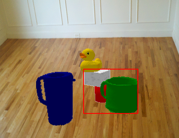
(b)

Figure 6: Examples of ROIs automatically identified by the attention mechanism for further analysis in the context of estimating: (a) stability of object structures; and (b) occlusion of objects.

As an example, consider the task of determining the stability of object structures in the image in Figure 6(a). Axioms that define conditions under which a particular object is considered to be stable, and those that define conditions under which an object is considered to be unstable, are relevant to this task. These axioms would have $stable(A)$ or $\lnot stable(A)$ in the head of the axiom, e.g., Statement 8(a) and Statement 9 respectively in Section 3.4 below. The head of any such axiom holds true in any state in which all the relations in the body of the axioms are satisfied. In the case of Statement 8(a) and Statement 9, the body of the axiom contains the spatial relation $above$, leading the attention mechanism to consider the stack comprising the duck, the red can, and the white cube, as indicated by the red rectangle in Figure 6(a), because they satisfy the relevant relation. While this ROI is analyzed further, other image regions and objects (e.g., mug, pitcher) are disregarded. Note that the process of selecting axioms in the knowledge base relevant to any given task, and extracting image ROIs satisfying the body of these axioms, is fully automated; there is no manual intervention.

As another example, consider the task of identifying occluded objects in Figure 6(b). Statement 8(b) in Section 3.4, which defines conditions under which an object is not considered to be occluded (as indicated by the axiom’s head), is relevant to the task. This axiom’s body indicates that the relation $behind$ is relevant for decisions about occlusion of objects, and the attention mechanism will only consider pairs of objects in Figure 6(b) that satisfy this relation. The red rectangle in Figure 6(b) indicates the relevant image region comprising the mug, the red can, and the white cube. This region is analyzed further, whereas the other image regions are disregarded. As before, this selection of the ROI is achieved without any manual supervision.

Once the attention mechanism identifies image ROIs enveloping objects that could not be assigned stability and occlusion labels using ASP-based reasoning, pixels of each such ROI are considered to provide information that is relevant to the estimation tasks but is not captured by the existing knowledge base (i.e., ASP program). The pixels in these ROIs and the target labels to be assigned to objects (and structures) in the ROIs are provided as inputs to a CNN. The CNN learns the mapping between the image pixels and target labels, and then assigns these labels to ROIs in previously unseen test images that ASP-based reasoning is unable to process.

A CNN has many parameters based on size, number of layers, activation functions, and the connections within and between layers, but the basic building blocks are convolutional, pooling, and fully-connected layers. The convolutional and pooling layers are used in the initial or intermediate stages of the network, whereas the fully-connected layer is typically one of the final layers. In a convolutional layer, a filter (or kernel) is convolved with the original input (to the network) or the output of the previous layer. One or more convolutional layers are usually followed by a pooling layer. Common pooling strategies such as max-pooling and average-pooling are used to reduce the dimensions of the input data, limit the number of parameters, and control overfitting. The fully-connected layers are equivalent to feed-forward neural networks in which all neurons between adjacent layers are connected—they often provide the target outputs. In the context of images, convolutional layers extract useful attributes to model the mapping from inputs to outputs, e.g., the initial layers may extract lines and arcs, whereas the subsequent layers may compose more complex geometric shapes. While estimating the stability of object configurations, the CNN’s layers may implicitly represent attributes such as whether: (i) a tower of blocks is aligned; (ii) an object with an uneven surface is under another object; or (iii) a tower has a small base.

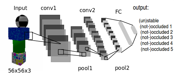
Figure 7: Lenet architecture.

In this paper, we adapt and use two established CNN architectures: (i) Lenet [33], initially proposed for recognizing hand-written digits; and (ii) Alexnet [29], which has been used widely since it provided very good results on the Imagenet benchmark dataset. The Lenet has two convolutional layers, each one followed by a max-pooling layer and an activation layer. Two fully connected layers are placed at the end. Unlike the $28\times 28$ gray-scale input images and the ten-class softmax output layer used in the original implementation, we consider $56\times 56$ RGB images as the input. Note that each such input to the network corresponds to an image ROI under consideration. The input vector size was chosen experimentally using validation sets and ROIs were scaled appropriately; the minimal improvement in performance provided by longer input vectors did not justify the significant increase in computational effort. The network’s outputs estimate the occlusion of each object and the stability of object structure(s) in the ROI under consideration. As described later in Section 4.1, we consider ROIs with up to five objects, and we use the sigmoid activation function. Figure 7 is a pictorial representation of this network. The Alexnet architecture, on the other hand, contains five convolutional layers, each followed by max-pooling and activation layers, along with three fully connected layers at the end. In our experiments, each input vector is a $227\times 227$ RGB image. The size of the output vector and the activation function are the same as those for the Lenet architecture.

With both CNN architectures, we used the Adam optimizer [27] in TensorFlow [1] with a learning rate of $0.0002$ and $0.0001$ for Lenet and Alexnet respectively; the initial weights were initialized randomly. The number of training iterations varied depending on the network and the number of training examples. For example, the Lenet network using $100$ ($5000$) image samples was trained for $10000$ ($40000$) iterations, whereas the Alexnet with $100$ ($5000$) training samples was trained for $8000$ ($20000$) iterations. The learning rate and number of iterations were chosen experimentally using validation sets. The number of epochs was chosen as the stopping criteria, instead of the training error, in order to allow the comparison between networks learned with and without the attention mechanism. The code for training the deep networks is in our open source repository [40]. Note that other, potentially more sophisticated, deep network models could be used in our overall architecture (instead of Lenet or Alexnet), but this is beyond the scope of this work. Also, the chosen CNN architectures are sufficient for the learning task when it is informed by reasoning with commonsense knowledge.

Recall that a CNN is only trained on ROIs from images for which ASP-based reasoning provides an incorrect outcome or is unable to provide an outcome. We consider any such trained CNN to represent previously unknown knowledge not encoded, or encoded incorrectly, in the ASP program. In other words, the observed incorrect outcome or lack of any outcome is considered to be a consequence of reasoning with incomplete or incorrect knowledge, which (in turn) can be because the knowledge was incomplete or incorrect when it was encoded initially, or because of changes in the domain over time. The next component of our architecture supports the incremental acquisition of previously unknown state constraints from the ROIs (used to train the deep networks), and the merging of this information with the existing knowledge. This process also (indirectly) helps understand the behavior of the trained deep networks.

3.4 Decision Tree Induction and Axiom Merging

In our architecture, previously unknown domain knowledge is learned incrementally using decision tree induction, and a heuristic approach inspired by human forgetting merges the learned knowledge with the existing knowledge for subsequent reasoning. As stated in Section 1, we illustrate this capability in this paper by learning axioms that represent previously unknown state constraints. In other work, we have demonstrated the use of the inductive learning approach, without the heuristic merging strategy, to learn other kinds of axioms [41].

We adapt the well-known ID3 algorithm [48] to construct the desired decision trees, using entropy minimization as the criterion to select the attribute to split the nodes. Building on the underlying distributed, relational representation of axioms, we learn separate decision trees for each estimation task, e.g., in the RA domain, we learn separate decision trees for stability estimation and occlusion estimation. The difference in the construction of these decision trees is in the use of the relational descriptions based on prior knowledge and the observations as the attributes. Specifically, relational domain attributes are extracted automatically from the image ROIs used for training the deep networks; recall that these attributes include the spatial relations between pairs of objects and the attributes of the objects in each such ROI. This relational information and the corresponding occlusion and stability labels are used as the labeled training examples to build the decisions trees for the estimation tasks under consideration. For the illustrative example domain considered in this paper, each tree’s nodes encode splits based on the domain attributes, and the labels of the leaf nodes are stable, unstable, occluded, and not occluded.

Once the decision trees are constructed, our approach automatically extracts candidate axioms from the trees. Consider, for example, the branches highlighted in gray in Figures 8 and 9, which show part of the decision trees learned in the RA domain. These branches can be translated to the axioms:

$$holds(stable(A),I)\leftarrow\ not~{}holds(obj\_relation(above,A,B),I)$$ (8a)

$$\neg holds(occluded(A),I)\leftarrow\ not~{}holds(obj\_relation(behind,A,B),I)$$ (8b)

where Statement 8(a) implies that any object that is not known to be above any other object is considered to be stable, whereas Statement 8(b) says that an object is not occluded if it is not known to be behind any other object. Note that this translation from the decision tree to axioms uses default negation to model the use of quantifiers with specific negated literals in the body of axioms. As another example, the branch highlighted in gray and blue in Figure 8 translates to the following axiom:

$$\neg holds(stable(A),I)~{}\leftarrow~{} holds(obj\_relation(above,A,B),I),\ obj\_surface(B,irregular)$$ (9)

which states that an object is unstable if it is located above another object with an irregular surface.

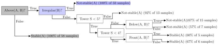
Figure 8: Example of a decision tree constructed for stability estimation using some labeled examples. Highlighted branches are used to construct previously unknown axioms.

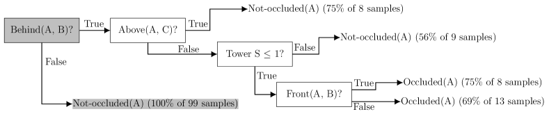
Figure 9: Example of a decision tree constructed for occlusion estimation using some labeled examples. Highlighted branch is used to construct previously unknown axiom.

1

Input : Relational domain attributes from image ROIs; occlusion and stability labels of objects in ROIs; thresholds $th_{1}$ ($95\%$, purity threshold), $th_{2}$ ($5\%$, support threshold), $th_{3}$ ($40\%$, tree support threshold), $th_{4}$ ($10\%$, axiom strength threshold); ensemble_count ($100$).

2

Output : Learned axioms.

3

4while true do

5      

6      if labeled_samples then

7            

8            for $j=1:ensemble\_count$ do

                   // Split training samples for learning and validation

9                   training_set, validation_set = random_split(labeled_samples)

10                  

                  // Decision tree induction

11                   learned_tree = tree_induction(training_set)

12                  

                  // Create candidate axioms

13                   candidate_axioms = select(learned_tree, $th_{1}$, $th_{2}$)

14                  

                  // Validate axioms

15                   validated_axioms = validate(candidate_axioms, validation_set, $th_{2}$)

16                  

17             end for

            // Choose validated axioms with sufficient support

18             axioms $=$ select(validated_axioms, $th_{3}$)

19            

            // Add validated axioms and merge similar axioms

20             add_merge(axioms)

21            

22       end if

23      

      // Update strength of axioms

24       update_strength(axioms)

25      

      // Remove axioms with low strength

26       remove(axioms, $th_{4}$)

27      

28 end while

Algorithm 1 Learning and merging axioms

Algorithm 1 describes the steps for automatically constructing the decisions trees, extracting and validating candidate axioms, and merging the valid new axioms with the existing knowledge. The algorithm first checks for suitable labeled training examples, i.e., image ROIs for which the stability and occlusion labels could not be determined correctly using ASP-based reasoning; these are used to induce new state constraints (lines 2-11). Specifically, a training set is created by randomly selecting $50\%$ of the labeled examples, with the remaining examples making up the validation set (line 4). As stated earlier, the construction of the tree is based on the ID3 algorithm [48]; it considers the relational attributes extracted from the image ROIs under consideration to split nodes, and assigns the known labels to the leaves. During the construction of the tree, the algorithm computes the potential change in entropy (i.e., information gain) that would occur if a split is introduced at a node in the tree based on each attribute that has not yet been used (line 5); the attribute that is likely to provide the highest reduction in entropy is selected to split the examples at a node.

Given any such tree, the branches of the tree (from root to leaves) that satisfy certain minimum requirements are selected to construct candidate axioms (line 6). These minimum requirements include thresholds on purity of samples at any given leaf, and on the support from the labeled examples, e.g., $\geq 95\%$ examples at the leaf belong to a particular (correct) label, and a branch under consideration has support from $\geq 5\%$ of the training samples. The selected branches of the learned decision trees represent previously unknown candidate constraints, and the thresholds are set to construct such candidate axioms cautiously, i.e., small changes in the value of these thresholds do not cause any significant change in the branches of the tree selected to construct axioms. The values of these thresholds can also be revised intentionally to achieve different desired behavior. For instance, to identify default constraints that hold in all but a few exceptional circumstances (see Section 3.2.2), we lower the threshold for selecting a branch of a tree to construct candidate axioms (from $95\%$ to $70\%$). As we will discuss later, lowering the thresholds results in the discovery of additional axioms, but also introduces noise. In addition, in this paper, learning of axioms containing default negation literals is restricted to default constraints such as Equation 3.2.2. In other words, the default negation is only associated with a literal in the body that is the negation of the literal in the head. This restriction is imposed primarily for computational efficiency because associating default negation with all literals would significantly increase the search space. Also, in any particular domain, the default negation is only applicable to certain literals, and this knowledge can be used during axiom learning. So, we demonstrate the capabilities of our approach with this restriction.

Once the candidate axioms are constructed, each one is validated using the other half of the labeled examples that have (so far) not been seen by the algorithm (line 7). The validation process removes axioms without a minimum level of support (e.g., $5\%$) from the labeled examples. Since the number of labeled examples available for training is often small, we reduce the effect of noise through a homogeneous ensemble learning approach (lines 3-8), i.e., we repeat the learning and validation steps a number of times (e.g., $100$) and only the axioms identified in more than a minimum number of iterations (e.g., $40\%$, line 9) are retained. Adding all retained axioms can lead to the ASP program including different versions of the same axiom over time. For instance, two axioms may have identical heads with one axiom’s body containing all the literals of the other, or two ground axioms may include sorts that are subsorts of a more general sort. To address this issue the algorithm reasons with the existing knowledge to identify the axioms to be added to the knowledge base ($add\_merge(axioms)$, line 10). First, axioms with the same head and overlap in the body are grouped together. Each possible combination of axioms from different groups (one from each group at a time) is then encoded in an ASP program along with the axioms that do not belong to any such group. The resulting program is used to classify ten labeled scenes chosen randomly. Axioms in the program that results in the highest accuracy are retained whereas the other axioms in each group are discarded.

The axiom learning approach described so far is based on a small number of labeled examples in a dynamic domain. The learned axioms may be incorrect (e.g., incorrect negation in the head, or incorrect literals in the body), incomplete (e.g., one or more missing literals in the body), or over-specified (e.g., one or more irrelevant literals in the body). Reasoning with these axioms can lead to sub-optimal or incorrect behavior. To address this issue, we incorporated a heuristic approach inspired by the human forgetting behavior [13]. This approach associates a “strength” values to each axiom. An axiom’s strength is revised over time based on a decay factor using an exponential relation: $axiom\_relevance=e^{-\alpha.n}$, where $\alpha$ represents the decay factor (initially $1$), and $n$ is the number of time steps since the axiom was learned. In each time step, irrespective of whether any new axioms are learned, the strength of all learned axioms are updated (line 12). If an axiom is reinforced, i.e., learned again or used, its strength is elevated to the maximum value (i.e., $1$) again, and its decay factor is divided by $\sqrt[n]{2}$, a value chosen experimentally such that it varies between 2 (for $n=1$) and 1 (for $n\rightarrow\infty$). Any axiom whose strength value falls below a threshold (e.g., $0.1$) is removed from further consideration (line 13).

4 Experimental Setup and Results

In this section, we first describe the experimental setup for evaluating our architecture (Section 4.1). We also specify the hypotheses to be evaluated for the: (a) incremental grounding of spatial relations; and (b) the estimation of object occlusion and the stability of object structures. Section 4.2 describes some execution traces and Section 4.3 discusses the results of experimental evaluation.

As stated in Section 1, our focus is on exploring the interplay between reasoning and learning for reliable and efficient operation in any given dynamic domain with a limited number of labeled training examples. Benchmark datasets that include a large number of images from different domains and approaches that do not support the desired coupling between representation, reasoning, and learning are thus not used for experimental evaluation. Instead, our experimental evaluation uses a limited number of real-world and simulated images from the domain under consideration, and considers ablation studies and architectures based just on deep networks as baselines for experimental evaluation.

4.1 Experimental Setup

We first describe the experimental set up, datasets, and the hypotheses for experimental evaluation. We do so separately for the incremental grounding of spatial relations (Section 4.1.1) and the estimation of object occlusion and stability (Section 4.1.2).

4.1.1 Incremental Grounding

For evaluating the grounding of spatial relations, we used the Table Object Scene Database (TOSD), with $111$ scenes for training and $131$ scenes for testing. TOSD contains scenes of real objects on a tabletop for evaluating segmentation algorithms. Many scenes include complex object configurations, e.g., Figure 10(b), while some scenes have only two objects, e.g., Figure 10(a). We chose this dataset because it provides a good combination of simple and complex scenes, and has been used as a benchmark in other work on segmentation and grounding of spatial relations. Since TOSD does not include spatial relation labels, we manually labeled the relations between objects in $200$ scenes. We then experimentally evaluated the following hypothesis:

1. The combination of manually-encoded QSR grounding and incrementally-learned MSR grounding performs better than each grounding used individually, and enables more effective use of human feedback.

The performance measure for evaluating this hypothesis was the accuracy of the labels assigned to the spatial relations between objects in the scene under consideration. Note that the labels assigned manually before the experimental evaluation provided the ground truth, and the human feedback provided during the experiments was in the form of labels for spatial relations between pairs of objects.

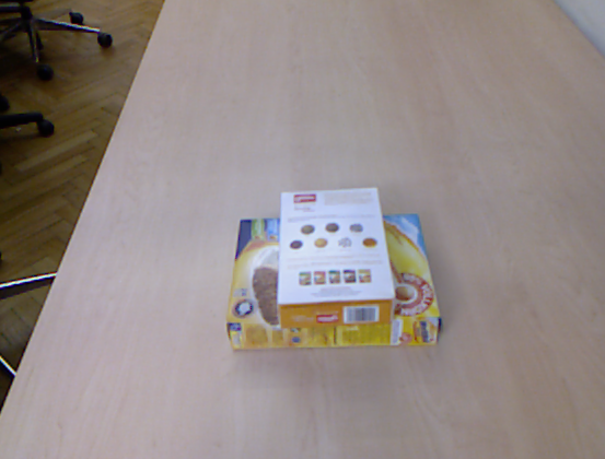
(a) Scene with two objects.

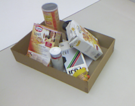
(b) Complex scene with multiple objects.

Figure 10: Examples of images from the TOSD dataset.

4.1.2 Occlusion and Stability Estimation

For evaluating the assignment of occlusion and stability labels to objects and object structures, we used a real-time physics engine (Bullet physics library) to generate $6000$ images. The objects we simulated included cylinders, spheres, cubes, a duck, and five objects from the Yale-CMU-Berkeley dataset (apple, pitcher, mustard bottle, mug, and cracker box) [8]. Objects were characterized by different colors, textures, and shapes. We considered three different arrangements of these objects:

• Towers: images containing $2-5$ objects stacked on top of each other;

• Spread: images with five objects placed in different relative positions on a flat surface; and

• Intersection: images with $2-4$ objects stacked on each other, with the rest ($1-3$ objects) on a flat surface.

The vertical alignment of stacked objects was randomized creating either a stable or an unstable arrangement. The horizontal distance between objects was also randomized, creating scenes with complex, partial, or no occlusion. Lighting, orientation, camera distance, camera orientation, and background, were also randomized. An additional $600$ labeled simulated scenes were also created and used for evaluation, e.g., for the approach to update the strength of the learned axioms. In addition, in the experimental trials summarized below, the ASP program was initially missing three state constraints (each) related to stability estimation and occlusion estimation.

A second dataset was derived from the dataset described above to represent information about ROIs in the input images. Recall from Section 3.3 that the attention mechanism module automatically extracts ROIs from input images that could not be labeled using ASP-based reasoning, by identifying relevant axioms and relations in the ASP program. Given the object arrangements described above, any ROI in any given image can have up to five objects. The second dataset automatically assigned labels to different possible ROIs in the images, which is used as the ground truth. During experimental evaluation, the application of the attention mechanism on any given image identified objects of interest in this image. The corresponding ROI from the second dataset was identified and the information from this ROI was analyzed instead of information from the entire image.

As baselines, the CNN architectures (Alexnet, Lenet) were trained and evaluated on the first dataset without our reasoning and attention mechanism modules. These were compared against the performance of our architecture for different number of training samples. Recall that occlusion is estimated for each object (i.e., maximum of five outputs for a ROI) and stability is estimated for each object structure (i.e., one output for each structure/ROI). The following hypotheses were evaluated experimentally:

1. Reasoning with commonsense domain knowledge and the attention mechanism to guide deep learning improves accuracy in comparison with the baselines.

2. Reasoning with commonsense domain knowledge and the attention mechanism to guide deep learning reduces sample complexity and thus the computational effort in comparison with the baselines.

3. Our architecture is able to incrementally learn previously unknown axioms, and using these axioms improves the accuracy of decision making in comparison with reasoning without the learned axioms.

4. Our approach for revising the strength of axioms and merging similar axioms is able to identify and remove incorrect axioms.

The main performance measures were the accuracy of the labels assigned to objects and objects structures, and correctness of the axioms learned and retained in the ASP program. Unless stated otherwise, all claims are statistically significant at $95\%$ significance level. Before we discuss the quantitative experimental results, we first describe the working of our architecture using execution traces.

4.2 Execution Trace

The following two execution traces illustrate the reasoning, axiom learning, and axiom merging capabilities of our architecture.

Execution Example 1

[Planning and learning]
Consider the scenario showed in Figure 6. The robot is given the goal of placing the red can on top of the white block, i.e., holds(relation(on, red_can, white_block), I). The agent initially does not know that an object placed on another object with an irregular surface is unstable, i.e, Statement 9, and creates the following plan:

1. Pick up the duck in step 0;

2. Put down the duck on the table in step 1;

3. Pick up the white cube in step 2;

4. Put down the white cube on the duck in step 3;

5. Pick up the red can in step 4;

6. Put down the red can on the white cube in step 5.

Since the robot is unaware of the state constraint represented by Statement 9, it observes the unexpected outcome of not having the white cube on the top of the duck after put it there, requiring a new plan after step 4. However, the robot learns from the unexpected observation and induces the previously unknown axiom (from the corresponding decision tree based on the relational representation). When asked to achieve the same goal from the same initial conditions, the robot computes the following plan:

1. Pick up the duck in step 0;

2. Put down the duck on the table in step 1;

3. Pick up the white cube in step 2;

4. Put down the white cube on the table in step 3;

5. Pick up the red can in step 4;

6. Put down the red can on the white cube in step 5.

The robot now avoids putting down the white cube (and thus the red can) on top of the duck that has irregular surface; executing this plan results in the goal being achieved. This example illustrates how learning previously unknown state constraints can help agents creating better plans. Table 6 shows quantitative results, which were obtained by considering multiple different scenarios and goals, to further support this conclusion.

Execution Example 2

[Axiom merging and generalization]
Consider an agent with the following rule in its knowledge base:

$$\neg occluded(A)\leftarrow\ not~{}obj\_relation(behind,A,B),obj\_relation(above,A,C)$$ (10)

This axiom is an over-specification of the axiom encoded by Statement 8(b); specifically, it contains the unnecessary literal $obj\_relation(above,A,C)$. Now, consider the situation in which the axiom learning approach has managed to extract a correct (ground) version of this axiom encoded by Statement 8(b). This invokes the axiom merging approach described in Section 3.4, which proceeds as follows.

• The robot compares the newly discovered axiom with the existing over-specified version (in Statement 10) to recognize that they are different version of the same axiom.

• The two axioms are placed in different ASP programs and tested (along with other axioms) in a number of different (artificially constructed) scenarios.

• The more general (i.e., concise) version of the axiom achieves better accuracy in these scenarios and the over-specified version is discarded.

• Recall that the axiom merging approach attributes an initial strength to learned axioms that decreases over time. If this strength falls bellow a threshold, the corresponding axiom is discarded. This helps retain only the relevant axioms for subsequent reasoning.

This example illustrates the working of Algorithm 1, and shows how it leverages the existing knowledge to learn and revise axioms.

4.3 Experimental Results

We next describe and discuss quantitative results corresponding to the evaluation of the hypotheses described in Section 4.1. The first set of experiments was designed to test the incremental grounding of spatial relations (i.e., hypothesis H1) as follows, using the setup procedure from Section 4.1.1, with the results summarized in Table 1:

1. Pairs of objects extracted from the training set of the TOSD were randomly divided into $10$ subsets.

2. Seven pairs of objects from each subset were used to train the MSR-based grounding with human feedback. Each pair represents one of the position-based spatial relations under consideration (i.e., in, left, right, front, behind, above, below).

3. Seven pairs of objects from each subset labeled with human feedback, and $200$ pairs with relations labeled using the QSR-based grounding, were used to train the MSR-based grounding.

4. The control node chose either the QSR-based grounding or the MSR-based grounding trained using the QSR-based grounding and human feedback.

The three schemes (in Steps 2-4 above) were evaluated on $200$ object pairs in test scenes of varying complexity. Table 1 indicates that the MSR-based grounding acquired using the QSR-based grounding makes better use of human feedback than the MSR-based grounding acquired using just human feedback, which supports hypothesis H1. Note that the same amount of human feedback is provided with the scheme in Step-2 and the scheme in Step-3. The difference is that the latter scheme bootstraps off the generic knowledge encoded in the QSR-based grounding. These results indicate that performance is improved by using prior knowledge, experience, and human feedback, and an appropriate representation for knowledge. Also, the control node-based combination of the two groundings (scheme in Step-4) provides better accuracy than just using the QSR-based approach (with accuracy of $70\%$ not shown in Table 1) or just using the MSR-based approach (scheme in Step-2). These results also support hypothesis H1.

	Accuracy of labels over test set of $200$ object pairs
Training sets	MSR (feedback)	MSR (QSR + feedback)	Combined model
Sets 1	65%	77%	84%
Sets 2	82%	80%	94%
Sets 3	68%	80%	85%
Sets 4	66%	83%	87%
Sets 5	65%	74%	82%
Sets 6	68%	77%	86%
Sets 7	64%	87%	90%
Sets 8	64%	84%	91%
Sets 9	62%	82%	87%
Sets 10	52%	72%	81%
Mean	65%	79%	87%
Std Dev	7.2%	4.6%	8.3%

Table 1: Comparison of three schemes (1) MSR-based grounding trained with just human feedback; (2) MSR-based grounding trained with 200 pairs labeled by the QSR-based grounding and seven pairs labeled with human feedback; and (3) the use of a control node to choose between the MSR-based grounding trained as in #2 and QSR-based grounding. The combined model supported by the third scheme provides significantly better performance than the other two schemes.

The subsequent experiments evaluated the ability of our architecture to assign occlusion and stability labels to objects and object structures in images, following the setup described in Section 4.1.2. Specifically, the second set of experiments was designed as follows, with results summarized in Figure 11:

1. Training datasets of different sizes ($100$, $200$, $1000$, and $5000$ images) were used to train the Lenet and Alexnet networks. The remaining images were used to test the learned models. Recall that the baseline CNNs do not use the attention mechanism or commonsense reasoning; the corresponding results are plotted as “Lenet” and “Alexnet” in Figure 11;

2. Another instance of the Lenet and Alexnet networks were trained and tested as part of our architecture, i.e., as directed by the reasoning module and the attention mechanism module. This training and testing considered the same images as in Step-1 but automatically identified the relevant ROIs and extracted the corresponding data from the second dataset described in Section 4.1.2. The corresponding results are plotted as “Lenet(Att)” and “Alexnet(Att)” in Figure 11.

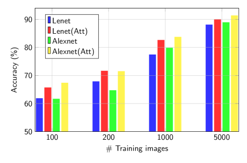
Figure 11: Accuracy of Lenet and Alexnet with and without commonsense reasoning and attention mechanism. Number of background images were $100$. Our architecture improves accuracy in comparison with the baselines.

Figure 11 indicates that reasoning with commonsense knowledge and using the attention mechanism to guide deep learning improves accuracy in comparison with the baselines (based on deep networks) for the estimation of stability and occlusion. Training and testing the deep networks with only relevant ROIs of images that cannot be processed by commonsense reasoning simplifies and directs the learning process. This approach helps learn an accurate mapping between inputs and outputs, resulting in higher accuracy than the baselines for any given number of training images. The improvement is more pronounced when the training set is smaller, but there is improvement at all training dataset sizes considered in our experiments. These results support hypothesis H2.

(a)

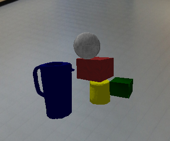
(b)

Figure 12: Test images for Lenet and Lenet(Att) architectures: (a) both networks detected the occlusion of the red cube by green mug, but only the latter correctly estimated the tower’s instability; and (b) both networks predicted the instability of the tower, but only Lenet(Att) detected the obstruction of green cube by yellow cylinder.

Figure 12 shows two specific instances of scenes in which the inclusion of commonsense reasoning and the attention mechanism improves performance. In Figure 12(a), both Lenet and Lenet(Att) were able to recognize the occlusion of the red cube caused by the green mug, but only the latter, which uses the attention mechanism and commonsense reasoning, was able to estimate the instability of the tower. In Figure 12(b), both networks correctly predicted the instability of the tower. However, only Lenet(Att) was able to identify the occlusion of the green cube by the yellow can. The classification errors of baselines architectures are primarily because a similar example had not been observed during training—this is a known limitation of deep network architectures. The attention mechanism eliminates the analysis of unnecessary parts of images and focuses only on the relevant parts, resulting in a more targeted network that provides better classification accuracy. For these experiments, the CNNs were trained with $1000$ images.

The number of different backgrounds (selected randomly) was fixed at $100$ for the experimental results in Figure 11. The effect of the background on the observed performance varies depending on the number of training examples. For instance, we had (on average) one image that used each background image when the training data had $100$ training samples, and we had $50$ images per background for the training dataset with $5000$ training examples. However, in real scenarios, it is unlikely that we will get a uniform distribution of backgrounds; other factors such as lighting, viewpoint, and orientation will be different in different images. To analyze the effect of different backgrounds, we explored the use of the Lenet architecture with different number of training examples ($100$ and $5000$) and different number of backgrounds ($30$, $50$, and $100$). As shown in Figure 13, varying the background did have an impact on accuracy, which degraded from $\approx 65\%$ for one background per $10$ images to $\approx 62\%$ when we had one background per image (i.e., $100$ backgrounds for $100$ images). The degradation was smaller, i.e., $\approx 1\%$, for $5000$ training examples with number of backgrounds varying from $10-100$; however, for $1000$ backgrounds (one background per five training images) the accuracy was reduced by $\approx 2\%$. These results indicate that a network trained with a larger number of images is less sensitive to variations in background, and that the inclusion of different backgrounds has a negative effect on the performance of the baseline (e.g., Lenet) architecture. On the other hand, with the inclusion of commonsense reasoning and the attention mechanisms, i.e., with Lenet(Att), classification accuracy similar over a range of the number of backgrounds, which indicates that our architecture provides some robustness to background variations.

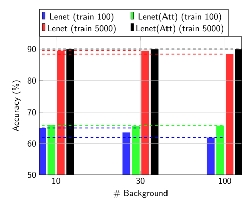
Figure 13: Effect of changing the number of backgrounds on the accuracy of the Lenet and Lenet(Att) networks for $100$ and $5000$ training images. Without the commonsense reasoning and attention mechanism, variations in the background influence the classification accuracy.

The third set of experiments was designed as follows to evaluate hypothesis H3 on the computational effort of training the deep networks in our architecture, with the corresponding results summarized in Figure 14:

1. The Lenet and Alexnet networks were trained with training datasets containing between $100-1000$ images, in step-sizes of $100$. Separate datasets were created for testing. Recall that the baseline deep networks do not include commonsense reasoning or the attention mechanism;

2. Another instance of the Lenet and Alexnet networks were trained and tested as part of our architecture, i.e., as directed by the reasoning module and the attention mechanism module. This training and testing considered the same images as in Step-1 but automatically identified the relevant ROIs and extracted the corresponding data from the second dataset described in Section 4.1.2. The corresponding results are plotted as “Lenet(Att)” and “Alexnet(Att)” in Figure 14.

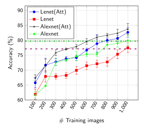
Figure 14: Accuracy of Lenet and Alexnet with and without the attention mechanism and commonsense reasoning. The number of background images was fixed at $100$. Any desired accuracy is achieved with a smaller training set when commonsense reasoning and the attention mechanism are used.

Figure 14 shows that using the attention mechanism and reasoning with commonsense knowledge helps achieve any desired level of accuracy with much fewer training examples. The purple dashed line in Figure 14 indicates that the baseline Lenet needs $\approx 1000$ images to reach an accuracy of $77\%$, whereas our architecture reduces this number to $\approx 600$. The experiments indicates a similar difference between the Alexnet and Alexnet(Att) for $79.5\%$ accuracy—see the dark green dash-dotted line in Figure 14. In other words, the use of commonsense knowledge helps train deep networks with fewer examples, reducing both the computational requirements and storage requirements. These results support hypothesis H3.

The fourth set of experiments was designed as follows to evaluate hypothesis H4, i.e., the ability to incrementally learn previously unknown axioms, with the corresponding results summarized in Table 2:

1. Ten sets of $50$ labeled images were created, as described in Section 4.1.2;

2. The axiom learning algorithm was trained with each set three times, using thresholds of $95\%$ and $70\%$ at the leaf nodes of the decision trees. These are the values assigned to threshold $th_{1}$ in the algorithm described in Table 1 in Section 3.4;

3. The precision and recall were computed for learning previously unknown axioms, e.g., Statements 8(a),  8(b), and 9, but excluding defaults and with threshold of $th_{1}=95\%$. The corresponding results are summarized as “unknown (normal)” in Table 2;

4. The precision and recall were computed for learning the unknown default statements, e.g., Statement 3.2.2 with threshold of $th_{1}=70\%$. The results are summarized as “unknown (default)” in Table 2.

In the results summarized in Table 2, errors were predominantly variants of the target axioms that were not in the most generic form, i.e., they had irrelevant literals but were not actually wrong. The lower precision and recall with defaults is understandable because it is challenging to distinguish between defaults and their exceptions. Although we do not describe it here, other studies indicated that reasoning with commonsense knowledge and decision trees can also be used to provide relational descriptions as (at least partial) explanations for the decisions made by the architecture [42].

Table 2: Precision and recall for learning previously unknown domain axioms (normal, default) using decision tree induction. It is possible to learn default constraints, but that also introduces errors.

Axiom type	Precision	Recall
Unknown (normal)	98%	100%
Unknown (default)	78%	62%

The fifth set of experiments were designed as follows to evaluate hypothesis H5 on revising and merging axioms, with results summarized in Figures 15 and 16 for non-default axioms and default axioms respectively:

1. Ten sets of $60$ labeled scenes were created, as described in Section 4.1.2. Each set was used in one run of ensemble learning (see Algorithm 1);

2. In each cycle, $50$ images were used for decision tree induction and axioms extraction. The other $10$ images supported the choice of the best version of similar axioms;

3. The decay factor and axiom strengths were updated, and the axioms with strength below $10\%$ were eliminated (orange dashed line in the figures below); and

4. Steps 2 and 3 were repeated for $10$ learning cycles.

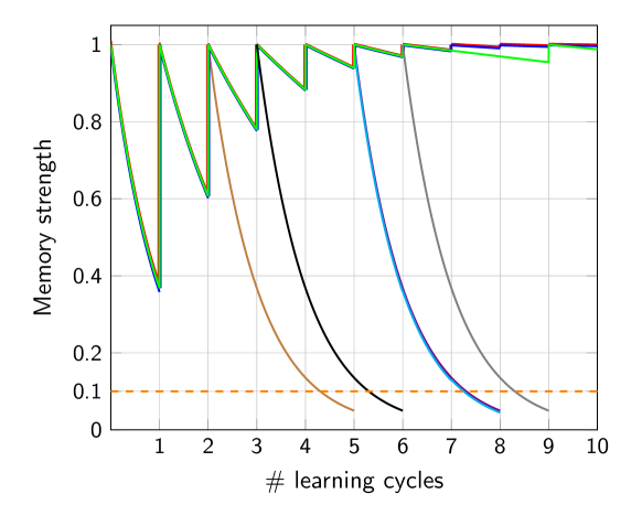
Figure 15: Evolution of the strengths of learned axioms (excluding defaults) over time.

Table 3: Learned axioms (excluding defaults) whose strengths are revised over time, as shown in Figure 15; ”obj_rel” is used as a short form of the relation ”obj_relation”, and each fluent $F$ is short form for $holds(F,I)$.

Color	Axiom	Discarded?
——	stable(A) :-  not  obj_rel(above,A,B),  $\lnot$ has_surface(A, irregular).	No
——	$\lnot$ occluded(A) :-  not  obj_rel(behind,A,B).	No
——	$\lnot$  stable(A) :-  irregular_below(A).	No
——	$\lnot$  occluded(A) :-  obj_rel(above,A,B).	Cycle 8
——	$\lnot$  stable(A) :-  obj_rel(above,A,B),  tower_height(A,N),  N$>$4.	Cycle 5
——	$\lnot$  stable(A) :-  small_base(A),  tower_height(A,N),  N$>$4.	Cycle 8
——	stable(A) :-  not  obj_rel(above,A,B),  obj_rel(behind,A,C).	Cycle 6
——	stable(A) :-  tower_height(A,N),  N$<=$1.	Cycle 9

Figure 15 shows how the strength of the eight axioms in Table 3 behaved over $10$ cycles. The top three axioms are shown in green, red, and blue; they are learned or reinforced in almost every cycle. Note that the first axiom corresponding to the green-colored plot is a variant of the axiom in Statement 8(a); it states that any object that is not above another object and does not have an irregular surface is stable. Although this axiom was not re-learned in learning cycles $7$ and $8$, it was able to maintain a high value of strength. This is because it was reinforced in all previous cycles, resulting in a small decay factor. In contrast, the other five axioms in Table 3 were not learned or used frequently. The strength of each of these axioms decreased over time and eventually fell below a threshold, causing the corresponding axiom to be removed. Figure 15 shows that our approach was able to identify and retain the correct axioms, and Figure 16 shows similar results for $10$ learned axioms (that included default statements) in Table 4. Note that among the learned axioms shown in Table 4, those on lines $4$ and $5$ (represented by brown and lime green-colored plots in Figure 16) are different versions of the same axiom. Specifically, the axiom on line $4$ has an extra (unnecessary) literal (holds(obj_relation(front, A, D), I)). When the similarity was identified, the axioms were merged by retaining the more general version, and the brown-colored plot stops after cycle $5$ in Figure 16. These results support hypothesis H5.

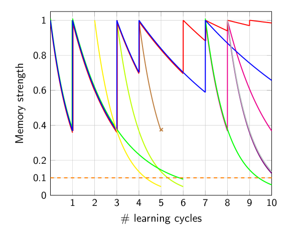
Figure 16: Evolution of the strengths of learned axioms (including defaults) over time.

Table 4: Learned axioms (including defaults) whose strengths are revised over time, as shown in Figure 16; ”obj_rel” is used as a short form of the relation ”obj_relation”, and each fluent $F$ is short form for $holds(F,I)$.

Color	Axioms	Discarded?
——	$\lnot$ stable(A) :-  small_base(A).	No
——	$\lnot$ stable(A) :-  obj_rel(above,A,B).	No
——	$\lnot$ stable(A) :-  tower_height(A,N), N$>$4.	No
——	occluded(A) :-  obj_rel(behind,A,B),  not obj_rel(above,A,C),  not obj_rel(front,A,D).	Cycle 5
——	occluded(A) :- obj_rel(behind,A,B),  not obj_rel(above, A, C).	Cycle 6
——	$\lnot$ occluded(A) :-  obj_rel(above,A,B).	Cycles 6, 10
——	stable(A) :-  not obj_rel(above,A,B).	No
——	stable(A) :-  obj_rel(behind,A,B).	No
——	stable(A) :-  obj_rel(front,A,B).	No
——	stable(A) :-  $\lnot$ small_base(A).	Cycle 5

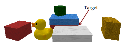
Figure 17: Illustrative image from the planning experiments with and without the learned axioms.

Table 5: Number of plans and planning time with the learned axioms expressed as a fraction of the values without the learned axioms. Reasoning with the learned axioms improves performance.

Measures	Ratio (with/without)
Number of plans	0.33
Planning time	0.89

Table 6: Number of optimal, sub-optimal, and incorrect plans expressed as a fraction of the total number of plans. Reasoning with the learned axioms improves performance.

Plans	Without	With
Optimal	0.15	0.49
Sub-optimal	0.31	0.51
Incorrect	0.54	0

The final set of experiments was designed as follows to evaluate the second part of hypothesis H4:

1. Forty initial object configurations were arranged; Figure 17 shows an illustrative example;

2. For each initial state, five goals were randomly chosen and encoded in the ASP program. The robot reasoned with the existing knowledge to create plans for these $200$ combinations ($40$ initial states, five goals);

3. The plans were evaluated in terms of the number of optimal, sub-optimal and incorrect plans, and the time taken to compute the plan; and

4. Experiments were repeated with and without the learned axioms.

Since the number of plans and planning time vary depending on the initial conditions and the goal, we conducted paired trials with and without the learned constraints included in the ASP program used for reasoning. The initial conditions and goal were identical in each paired trial, and differed between different paired trials. Then, we expressed the number of plans and the planning time with the learned constraints as a fraction of the corresponding values obtained by reasoning without the learned constraints. The average of these fractions over all the trials is reported in Table 5. In addition, we computed the number of optimal, sub-optimal, and incorrect plans in each trial as a fraction of the total number of plans in the trial; we did this separately with and without using the learned axioms for reasoning, and the average over all trials is summarized in Table 6. These results indicate that using the learned axioms for reasoning significantly reduced the search space, resulting in a much smaller number of plans and a substantial reduction in the planning time. In addition, when the robot used the learned axioms for reasoning, it resulted in a much smaller number of sub-optimal plans and eliminated all incorrect plans. Also, each such sub-optimal plan was created only when the corresponding goal could not be achieved without creating an exception to a default, e.g., stacking an object on a small base. Without the learned axioms, a larger fraction of the plans are sub-optimal or incorrect. These results support hypothesis H4.

As a specific example of the planning trials, the goal in one trial was to move the large red box partially hidden behind the white box and the duck in Figure 17 such that it is no longer occluded. With all the axioms the robot found eight plans (all of which were correct); however, with some axioms missing, the robot found as many as $90$ plans, many of which were incorrect. A plan was considered to be correct if executing it (in simulation) resulted in the corresponding goal being achieved.

5 Conclusions

Deep network architectures and algorithms represent the state of the art for many tasks in robotics and AI. However, they require large labeled training datasets and considerable computational resources, and it is difficult to understand the decisions made by the learned networks. The architecture described in this paper draws inspiration from research in cognitive systems to address these limitations. Instead of focusing of generalizing across domains, our architecture integrates the complementary principles of deep learning, non-monotonic logical reasoning with commonsense knowledge, and decision tree induction of knowledge for reliable and efficient reasoning and learning for any given domain. The underlying intuition is that commonsense knowledge is available in almost every application domain—in fact, some such knowledge is often used implicitly or explicitly to optimize the parameters of deep networks. Our architecture seeks to fully exploit this knowledge. Reasoning with domain knowledge simplifies learning—the robot only needs to learn aspects of the domain not already encoded, or encoded incorrectly, by the existing knowledge. A more accurate mapping is thus learned between the desired inputs and outputs using a smaller set of labeled examples and based on fewer attributes. We have experimentally validated our intuition in the context of estimating the occlusion of objects and the stability of object structures in simulated and real-world images. Our architecture improves accuracy, and reduces storage and computation requirements, especially when large labeled training datasets are not available.

The architecture described here opens up multiple directions for future research. First, we will consider more complex scenes with more objects and clutter, e.g., by including more complex real-world images from the TOSD dataset similar to the image in Figure 10(b), in our experiments on estimating occlusion and stability. We hypothesize that our architecture will scale to such scenes because it reasons with, and learns from, only the relevant information in the scene. Second, we will further explore the interplay between reasoning and learning to better understand the operation of deep network models. We have already shown in other work that the use of relational logical structures makes it easier to explain the decisions, the underlying knowledge and beliefs, and the experiences that informed these beliefs [42]. We will now explore the use of different deep network architectures, and use the corresponding learned axioms to better understand the behavior of the deep networks. Note that our architecture’s ability to selectively train the deep networks on a subset of images also simplifies the process of exploring the behavior of these networks. Third, we will expand the learning capabilities of our architecture to learn other kinds of axioms. Recall that we have only discussed the learning of state constraints in this paper, although the underlying representation supports other kinds of axioms as well. Other work in our group has demonstrated the use of relational reinforcement learning, inductive learning, and limited human feedback for learning different types of axioms [41, 55]. Incorporating the ability to learn different axioms in our architecture will significantly enhance our ability to reason accurately and better explore the behavior of the deep networks. Furthermore, we will explore the use of this architecture on robots assisting humans in complex domains, reasoning with relevant information at different resolutions [54], and providing relational descriptions as explanations for their decisions and beliefs during reasoning and learning.

Declarations

Funding: This work was supported in part by the Asian Office of Aerospace Research and Development award FA2386-16-1-4071. All opinions and conclusions described in this paper are those of the authors.

Conflict of interest/Competing interests: Not applicable.

Availability of data and material: The entire dataset of images used in our experiments is $\geq 100MB$ and point cloud data is $\geq 3GB$ in size. A link to most of the data is provided with our code repository (see below); we will make all the data available online after review.

Code availability: Please see [40].

Author contributions: TM and MS contributed to the design of the architecture and algorithms; TM implemented the algorithms; TM and MS designed the experiments; TM conducted the experiments and gathered experimental results; TM and MS analyzed the results; MS and TM wrote the paper.

References

- [1] M Abadi, A Agarwal, P Barham, E Brevdo, Z Chen, C Citro, GS Corrado, A Davis, J Dean, M Devin, et al. TensorFlow: large-scale machine learning on heterogeneous distributed systems. arXiv preprint arXiv:1603.04467, 2016.
- [2] Roy Assaf and Anika Schumann. Explainable Deep Neural Networks for Multivariate Time Series Predictions. In International Joint Conference on Artificial Intelligence, 2019.
- [3] Evgenii Balai, Michael Gelfond, and Yuanlin Zhang. Towards Answer Set Programming with Sorts. In International Conference on Logic Programming and Nonmonotonic Reasoning, Corunna, Spain, September 15-19, 2013.
- [4] Marcello Balduccini and Michael Gelfond. Logic Programs with Consistency-Restoring Rules. In AAAI Spring Symposium on Logical Formalization of Commonsense Reasoning, pages 9–18, 2003.
- [5] Peter W Battaglia, Jessica B Hamrick, and Joshua B Tenenbaum. Simulation as an engine of physical scene understanding. Proceedings of the National Academy of Sciences, pages 18327–18332, 2013.
- [6] Anja Belz, Adrian Muscat, Maxime Aberton, and Sami Benjelloun. Describing spatial relationships between objects in images in english and french. Proceedings of the 2015 Workshop on Vision and Language, 15:104–113, September 2015.
- [7] Tarek R Besold, Artur d’Avila Garcez, Sebastian Bader, Howard Bowman, Pedro Domingos, Pascal Hitzler, Kai-Uwe Kühnberger, Luis C Lamb, Daniel Lowd, Priscila Machado Vieira Lima, et al. Neural-symbolic learning and reasoning: A survey and interpretation. arXiv preprint arXiv:1711.03902, 2017.
- [8] Berk Calli, Aaron Wallsman, Arjun Singfh, and Siddhartha S. Srinivasa. Benchmarking in Manipulation Research. IEEE Robotics and Automation Magazine, pages 36–52, 2015.
- [9] J. Y. Chai, Q. Gao, L. She, S. Yang, S. Saba-Sadiya, and G. Xu. Language to Action: Towards Interactive Task Learning with Physical Agents. In International Joint Conference on Artificial Intelligence (IJCAI), Stockholm, Sweden, July 13-19, 2018.
- [10] Eugene Charniak. On the use of framed knowledge in language comprehension. Artificial Intelligence, 11(3):225–265, 1978.
- [11] Simon Dobnik, Mehdi Ghanimifard, and John Kelleher. Exploring the functional and geometric bias of spatial relations using neural language models. In Proceedings of the Combined Workshop on Spatial Language Understanding (SpLU) and Grounded Communication for Robotics (RoboNLP), pages 1–11, 2018.
- [12] Desmond Elliott and Arjen P De Vries. Describing Images using Inferred Visual Dependency Representations. Acl, pages 42–52, 2015.
- [13] Thomas Ellwart and Annette Kluge. Psychological perspectives on intentional forgetting: An overview of concepts and literature. KI-Künstliche Intelligenz, 33(1):79–84, 2019.
- [14] Esra Erdem, Michael Gelfond, and Nicola Leone. Applications of Answer Set Programming. AI Magazine, 37(3):53–68, 2016.
- [15] Esra Erdem and Volkan Patoglu. Applications of ASP in Robotics. Kunstliche Intelligenz, 32(2-3):143–149, 2018.
- [16] Severin Fichtl, Dirk Kraft, Norbert Krüger, and Frank Guerin. Using relational histogram features and action labelled data to learn preconditions for means-end actions. In IEEE/RSJ International Conference on Intelligent Robots and Systems (Workshop on Sensorimotor Contingencies for Robotics), Hamburg. Citeseer, 2015.
- [17] Katerina Fragkiadaki, Pulkit Agrawal, Sergey Levine, and Jitendra Malik. Learning visual predictive models of physics for playing billiards. arXiv preprint arXiv:1511.07404, 2015.
- [18] Artur S. d’Avila Garcez, Luis C Lamb, and Dov M Gabbay. Connectionist modal logic: Representing modalities in neural networks. Theoretical Computer Science, 371(1-2):34–53, 2007.
- [19] Yiannis Gatsoulis, Muhannad Alomari, Chris Burbridge, Christian Dondrup, Paul Duckworth, Peter Lightbody, Marc Hanheide, Nick Hawes, DC Hogg, and AG Cohn. Qsrlib: a software library for online acquisition of qualitative spatial relations from video. In International Workshop on Qualitative Reasoning at IJCAI, New York, USA, July 2016.
- [20] Michael Gelfond and Daniela Inclezan. Some Properties of System Descriptions of . Journal of Applied Non-Classical Logics, Special Issue on Equilibrium Logic and Answer Set Programming, 23(1-2):105–120, 2013.
- [21] Michael Gelfond and Yulia Kahl. Knowledge Representation, Reasoning and the Design of Intelligent Agents. Cambridge University Press, 2014.
- [22] Yolanda Gil. Learning by Experimentation: Incremental Refinement of Incomplete Planning Domains. In International Conference on Machine Learning, pages 87–95, New Brunswick, USA, July 10-13, 1994.
- [23] Rocio Gomez, Mohan Sridharan, and Heather Riley. What do you really want to do? Towards a Theory of Intentions for Human-Robot Collaboration. Annals of Mathematics and Artificial Intelligence, special issue on commonsense reasoning, 89:179–208, Februray 2021.
- [24] R. H. J. Granger. Adaptive Understanding: Correcting Erroneous Inferences. PhD thesis, Yale University. Computer Science Department, 1980.
- [25] Mathieu Guillame-Bert, Krysia Broda, and Artur d’Avila Garcez. First-order logic learning in artificial neural networks. In The 2010 International Joint Conference on Neural Networks (IJCNN), pages 1–8. IEEE, 2010.
- [26] Philipp Jund, Andreas Eitel, Nichola Abdo, and Wolfram Burgard. Optimization Beyond the Convolution: Generalizing Spatial Relations with End-to-End Metric Learning. In ICRA, 2018.
- [27] Diederik P Kingma and Jimmy Ba. Adam: A method for stochastic optimization. arXiv preprint arXiv:1412.6980, 2014.
- [28] Nikhil Krishnaswamy, Scott Friedman, and James Pustejovsky. Combining deep learning and qualitative spatial reasoning to learn complex structures from sparse examples with noise. In AAAI Conference on Artificial Intelligence, volume 33, pages 2911–2918, 2019.
- [29] Alex Krizhevsky, Ilya Sutskever, and Geoffrey E Hinton. Imagenet classification with deep convolutional neural networks. In Advances in neural information processing systems, pages 1097–1105, 2012.
- [30] John E. Laird, Kevin Gluck, John Anderson, Kenneth D. Forbus, Odest Chadwicke Jenkins, Christian Lebiere, Dario Salvucci, Matthias Scheutz, Andrea Thomaz, Greg Trafton, Robert E. Wray, Shiwali Mohan, and James R. Kirk. Interactive Task Learning. IEEE Intelligent Systems, 32(4):6–21, 2017.
- [31] Mark Law, Alessandra Russo, and Kysia Broda. The Complexity and Generality of Learning Answer Set Programs. Artificial Intelligence, 259:110–146, 2018.
- [32] Mark Law, Alessandra Russo, and Kysia Broda. The ILASP System for Inductive Learning of Answer Set Program. Association for Logic Programming Newsletter, 2020.
- [33] Yann LeCun, Léon Bottou, Yoshua Bengio, and Patrick Haffner. Gradient-based learning applied to document recognition. Proceedings of the IEEE, 86(11):2278–2324, 1998.
- [34] Adam Lerer, Sam Gross, and Rob Fergus. Learning physical intuition of block towers by example. arXiv preprint arXiv:1603.01312, 2016.
- [35] Wenbin Li, Aleš Leonardis, and Mario Fritz. Visual stability prediction and its application to manipulation. arXiv preprint arXiv:1609.04861, 2016.
- [36] Robin Manhaeve, Sebastijan Dumancic, Angelika Kimmig, Thomas Demeester, and Luc De Raedt. DeepProbLog: Neural Probabilistic Logic Programming. In Advances in Neural Information Processing Systems (NeurIPS), Montreal, Canada, December 3-8, 2018.
- [37] Oier Mees, Nichola Abdo, Mladen Mazuran, and Wolfram Burgard. Metric learning for generalizing spatial relations to new objects. In IEEE/RSJ International Conference on Intelligent Robots and Systems, pages 3175–3182, 2017.
- [38] Tiago Mota and Mohan Sridharan. Incrementally Grounding Expressions for Spatial Relations between Objects. In International Joint Conference on Artificial Intelligence, Stockholm, Sweden, July 13-19, 2018.
- [39] Tiago Mota and Mohan Sridharan. Commonsense Reasoning and Knowledge Acquisition to Guide Deep Learning on Robots. In Robotics Science and Systems, Freiburg, Germany, June 22-26, 2019.
- [40] Tiago Mota and Mohan Sridharan. Software related to the paper, 2019. https://github.com/tmot987/Scenes-Understanding.
- [41] Tiago Mota and Mohan Sridharan. Axiom Learning and Belief Tracing for Transparent Decision Making in Robotics. In AAAI Fall Symposium on Artificial Intelligence for Human-Robot Interaction: Trust and Explainability in Artificial Intelligence for Human-Robot Interaction, November 13-14, 2020.
- [42] Tiago Mota, Mohan Sridharan, and Ales Leonardis. Integrated Commonsense Reasoning and Deep Learning for Transparent Decision Making in Robotics. Springer Nature Computer Science, 2(242):1–18, 2021.
- [43] Roozbeh Mottaghi, Mohammad Rastegari, Abhinav Gupta, and Ali Farhadi. ”What happens if..” Learning to Predict the Effect of Forces in Images. In European Conference on Computer Vision, pages 269–285. Springer, 2016.
- [44] Arvind Neelakantan, Quoc V Le, and Ilya Sutskever. Neural programmer: Inducing latent programs with gradient descent. arXiv preprint arXiv:1511.04834, 2015.
- [45] Rohan Paul, Jacob Arkin, Derya Aksaray, Nicholas Roy, and Thomas M Howard. Efficient grounding of abstract spatial concepts for natural language interaction with robot platforms. The International Journal of Robotics Research, 37(10):1269–1299, 2018.
- [46] Andrzej Pronobis and Rajesh Rao. Learning Deep Generative Spatial Models for Mobile Robots. In RSS Workshop on Spatial-Semantic Representations in Robotics, Cambridge, USA, July 16, 2017.
- [47] Senthil Purushwalkam, Abhinav Gupta, Danny Kaufman, and Bryan Russell. Bounce and learn: Modeling scene dynamics with real-world bounces. In International Conference on Learning Representations, 2019.
- [48] J. Ross Quinlan. Induction of decision trees. Machine learning, 1(1):81–106, 1986.
- [49] Heather Riley and Mohan Sridharan. Integrating Non-monotonic Logical Reasoning and Inductive Learning With Deep Learning for Explainable Visual Question Answering. Frontiers in Robotics and AI, special issue on Combining Symbolic Reasoning and Data-Driven Learning for Decision-Making, 6:20, December 2019.
- [50] Wojciech Samek, Thomas Wiegand, and Klaus-Robert Muller. Explainable Artificial Intelligence: Understanding, Visualizing and Interpreting Deep Learning Models. ITU Journal: ICT Discoveries: The Impact of Artificial Intelligence on Communication Networks and Services, 1:1–10, 2017.
- [51] Adam Santoro, David Raposo, David G Barrett, Mateusz Malinowski, Razvan Pascanu, Peter Battaglia, and Tim Lillicrap. A simple neural network module for relational reasoning. In Advances in neural information processing systems, pages 4967–4976, 2017.
- [52] Mohit Shridhar and David Hsu. Grounding Spatio-Semantic Referring Expressions for Human-Robot Interaction. In RSS Workshop on Spatial-Semantic Representations in Robotics, July 2017.
- [53] Herbert A. Simon and Glenn Lea. Problem Solving and Rule Induction: A Unified View. In Knowledge and Cognition, pages 15–26. Lawrence Eribaum, Oxford, UK, 1974.
- [54] Mohan Sridharan, Michael Gelfond, Shiqi Zhang, and Jeremy Wyatt. REBA: A Refinement-Based Architecture for Knowledge Representation and Reasoning in Robotics. Journal of Artificial Intelligence Research, 65:87–180, May 2019.
- [55] Mohan Sridharan and Ben Meadows. Knowledge Representation and Interactive Learning of Domain Knowledge for Human-Robot Collaboration. Advances in Cognitive Systems, 7:77–96, December 2018.
- [56] Russell Stewart and Stefano Ermon. Label-free supervision of neural networks with physics and domain knowledge. In Thirty-First AAAI Conference on Artificial Intelligence, 2017.
- [57] Niko Sünderhauf, Oliver Brock, Walter Scheirer, Raia Hadsell, Dieter Fox, Jürgen Leitner, Ben Upcroft, Pieter Abbeel, Wolfram Burgard, Michael Milford, et al. The limits and potentials of deep learning for robotics. The International Journal of Robotics Research, 37(4-5):405–420, 2018.
- [58] Akshaya Thippur, Chris Burbridge, Lars Kunze, Marina Alberti, John Folkesson, Patric Jensfelt, and Nick Hawes. A Comparison of Qualitative and Metric Spatial Relation Models for Scene Understanding. Aaai, (Section 4):1632–1640, 2015.
- [59] Morgan Ulinski, Bob Coyne, and Julia Hirschberg. Spatialnet: A declarative resource for spatial relations. In Proceedings of the Combined Workshop on Spatial Language Understanding (SpLU) and Grounded Communication for Robotics (RoboNLP), pages 61–70, 2019.
- [60] Misha Wagner, Hector Basevi, Rakshith Shetty, Wenbin Li, Mateusz Malinowski, Mario Fritz, and Ales Leonardis. Answering Visual What-If Questions: From Actions to Predicted Scene Descriptions. In Visual Learning and Embodied Agents in Simulation Environments (VLEASE) Workshop at ECCV, Munich, Germany, September 9, 2018.
- [61] Jiajun Wu, Ilker Yildirim, Joseph J Lim, Bill Freeman, and Josh Tenenbaum. Galileo: Perceiving physical object properties by integrating a physics engine with deep learning. In Advances in neural information processing systems, pages 127–135, 2015.
- [62] Jun Ye and Kien A Hua. Exploiting depth camera for 3D spatial relationship interpretation. Proceedings of the 4th ACM Multimedia Systems Conference on - MMSys ’13, pages 151–161, 2013.
- [63] Kexin Yi, Chuang Gan, Yunzhu Li, Pushmeet Kohli, Jiajun Wu, Antonio Torralba, and Joshua B. Tenenbaum. CLEVRER: CoLlision Events for Video REpresentation and Reasoning. In International Conference on Learning Representations, April 26 - May 1, 2020.
- [64] Kexin Yi, Jiajun Wu, Chuang Gan, Antonio Torralba, Pushmeet Kohli, and Joshua B. Tenenbaum. Neural-Symbolic VQA: Disentangling Reasoning from Vision and Language Understanding. In Neural Information Processing Systems, Montreal, Canada, December 3-8, 2018.
- [65] Konstantinos Zampogiannis, Yezhou Yang, Cornelia Ferm, and Yiannis Aloimonos. Learning the Spatial Semantics of Manipulation Actions through Preposition Grounding. In International Conference on Robotics and Automation, pages 1389–1396, May 2015.
- [66] Renqiao Zhang, Jiajun Wu, Chengkai Zhang, William T Freeman, and Joshua B Tenenbaum. A comparative evaluation of approximate probabilistic simulation and deep neural networks as accounts of human physical scene understanding. arXiv preprint arXiv:1605.01138, 2016.
- [67] Fatemeh Ziaeetabar, Eren Erdal Aksoy, Florentin Wörgötter, and Minija Tamosiunaite. Semantic Analysis of Manipulation Actions Using Spatial Relations. In International Conference on Robotics and Automation, pages 4612–4619, 2017.