A Nested Error Regression Model with High Dimensional Parameter for Small Area Estimation

Abstract

In this paper we propose a flexible nested error regression small area model with high dimensional parameter that incorporates heterogeneity in regression coefficients and variance components. We develop a new robust small area specific estimating equations method that allows appropriate pooling of a large number of areas in estimating small area specific model parameters. We propose a parametric bootstrap and jackknife method to estimate not only the mean squared errors but also other commonly used uncertainty measures such as standard errors and coefficients of variation. We conduct both model-based and design-based simulation experiments and real-life data analysis to evaluate the proposed methodology.

Keywords: design consistency; M-estimation; root mean squared error estimation; AAGIS data; EMAP data.

1 Introduction

Planning and evaluation of government programs require access to a wide range of national and sub-national socio-economic, environment, health, and other statistics. For this reason, there is a growing need for reliable statistics relating to much smaller geographical areas where data are too sparse to support the sort of standard estimation methods typically employed at the national level. These small area official statistics are routinely used for a variety of purposes, including assessing economic well-being of a nation, making public policies, and allocating funds at the federal, state and local levels.

The main idea behind small area estimation is to borrow strength from related sources through statistical models that connect different alternative databases. In much of the small area literature, mixed models are generally employed because such models can account for uncertainties from different sources and thereby can produce accurate estimates and associated uncertainty measures at granular levels compared to the corresponding fixed effects models. M-quantile regression can be considered as an alternative class of models for the same purpose relaxing some of the conventional modelling assumptions such as the normality of the random components and obtaining estimators that are robust against outlying values. We refer to the well-cited Wiley book by Rao and Molina, (2015) and papers by Jiang and Lahiri, (2006), Pfeffermann, (2013), Chambers et al., (2014), Ghosh, (2020), and Salvati et al., (2021) for a detailed account of different small area models and methods.

Battese et al., (1988) proposed an empirical best linear unbiased prediction (EBLUP) method, using a nested error regression (NER) model, in order to estimate acreage under corn and soybeans for 12 counties in north-central Iowa, USA. The nested error regression model, a special case of linear mixed model, can be viewed as an extension of a regression model where the intercept term is allowed to vary across counties (or small areas), but, in order to make the method efficient, the county specific intercepts are assumed to be generated from the same underlying distribution. This random area specific intercept term is introduced in order to capture a part of the leftover between county variation that is not explained by the area specific auxiliary variables included in the model. The associated EBLUP method borrows strength from the known auxiliary variable means for the area population.

The NER model has played an important role in small area estimation since the publication of Battese et al., (1988). However, such a model is likely to fail when the number of small areas to be combined is large. This is because the assumption of the same regression coefficients and/or variance components in the nested error regression model may not be tenable for all the small areas. Random area specific regression coefficients models, which extend the nested error model by treating regression coefficients as random effects, have been suggested in the literature; see Prasad and Rao, (1990), Hobza and Morales, (2013), Rao and Molina, (2015) for empirical best prediction (EBP) approach and Hoff, (2009) for the Bayesian approach. Such modeling, though useful in some applications, needs more nontrivial assumptions on the joint distribution on the random regression coefficients. Jiang and Nguyen, (2012) considered a heteroscedastic nested error regression model by allowing different fixed sampling variances. They showed that all the parameters, except the area specific sampling variances, of their model can be consistently estimated. Interestingly, their EBP does not involve area specific sampling variances because of the assumption that the variances of the random effects are proportional to the corresponding sampling variances. Thus, their EBP well approximates the corresponding best predictor (BP) when the number of areas is large. However, the model does not allow second-order unbiased MSE estimator since MSE involves sampling variances, which cannot be consistently estimated. Moreover, random area specific sampling variance models have been also proposed in order to incorporate the leftover between area heteroscedasticity of the sampling variances across areas not captured by the available auxiliary variables. Early examples of such models can be found in Otto and Bell, (1995) and Arora et al., (1997). For more recent research in modeling sampling variances as a way to incorporate heteroscedastic variances, see Liu et al., (2014), Kubokawa et al., (2016), Sugasawa et al., (2017), Naves et al., (2020), among others. Though not used, one can envision a random area specific regression coefficients model in conjunction with random area specific sampling variance model to capture variations in both regression coefficients and sampling variances.

The random area specific regression coefficients models and/or random area specific sampling variances models involve specifications of distributions of a large number of random effects. On the other hand, fixed effects assumptions on the area specific regression coefficients and sampling variances generally lead to unstable estimates of these fixed effects due to small area specific sample sizes (Jiang and Nguyen,, 2012). In this paper, we introduce a new approach that is not considered in the literature. Specifically, we assume fixed effects for both regression coefficients and sampling variances, but use area specific estimating equations applied to data from all areas in estimating these area specific regression coefficients and then use appropriately constructed residuals for estimation of variance components. The proposed model can be called a nested error regression with high dimensional parameter.

When area specific tuning parameters of the system of estimating equations are known, we have shown that parameters of our proposed nested error regression model with high dimensional parameter can be consistently estimated. This is because we use data from all areas in estimating any area specific model parameter. When the tuning parameters are unknown, we have suggested two different estimators of these parameters. However, for obtaining consistent estimators of the tuning parameters, a basic requirement would be large area specific sample sizes. However, like most papers in small area estimation, our emphasize here is small area specific sample sizes. Our extensive model-based and design-based simulation results demonstrate that our proposed estimation method performs well under a variety of simulation conditions.

Estimation of mean squared error (MSE) of EBLUP has been a topic of extensive research for more than the last three decades. The pioneering work of Prasad and Rao, (1990) inspired many in considering various extensions; see Datta and Lahiri, (2000), Das et al., (2004), Jiang et al., (2002) Hall and Maiti, (2006). In all these papers, the focus has been to derive second-order unbiased MSE estimators. In this paper, we are not requiring the second-order unbiasedness of MSE estimators for a couple of reasons. First, our goal here is to cover a wide range of uncertainty measures (e.g., Root MSE, CV, Relative RMSE) – not just MSE. What is second-order unbiased is not necessarily second-order unbiased for a nonlinear function of MSE. Second, existing second-order unbiased MSE estimates do not necessarily ensure strictly positive MSE estimates. As pointed out in Jiang et al., (2018) there is no paper in small area estimation that proves simultaneous properties of positivity and second-order unbiasedness of parametric bootstrap MSE estimates. The McJack method ensures both properties but only in estimating a known monotone function of MSE (e.g., logarithm of MSE) – not MSE. For these reasons, we have not attempted to develop second-order unbiased MSE estimators in this paper. We propose a simple general parametric bootstrap and a jackknife estimators of a wide range of uncertainty measures. We evaluate different uncertainty measures under different situations through extensive simulations. For known area specific tuning parameters, our estimators of uncertainty measures (not necessarily MSE) tend to the corresponding true uncertainty measures in probability.

The outline of the paper is as follows. In Section 2 we motivate the proposed nested error regression model with high dimensional parameter by analysing data from the US Environmental Protection Agency’s Environmental Monitoring and Assessment Program. After presenting notation and EBLUP estimators for small areas in Section 3, we propose a nested error regression models with high dimensional parameter in Section 4. In Section 5 we show its estimation algorithm, consistency property of the estimator and application to the SAE situation. In Section 6 we discuss two different estimators of the root mean squared errors of the proposed small area estimator. In particular, the first proposal is a parametric bootstrap estimator. The second MSE estimator is based on the Monte-Carlo jackknife method proposed by Jiang et al., (2018). In Section 7 we empirically evaluate the performance of the proposed approach and its associated MSE estimators using both model-based and design-based simulation studies, with the latter based on a real dataset: the 1995-96 Australian Agricultural Grazing Industry Survey (AAGIS) data (Chandra et al.,, 2012). In Section 8, we use the proposed method for estimating average levels of Acid Neutralising Capacity at 8-digit Hydrologic Unit Code (HUC) level using data collected in an environmental survey of lakes in the Northeast of the USA (Opsomer et al.,, 2008). Finally, in Section 9, we summarise our main findings and provide directions for future research.

2 A motivating example

To motivate the proposed nested error regression model with high dimensional parameter, we consider data from the US Environmental Protection Agency’s Environmental Monitoring and Assessment Program (EMAP) Northeast lakes survey (Larsen et al.,, 2001; Opsomer et al.,, 2008; Salvati et al., 2012b, ). Between 1991 and 1995, researchers from the US Environmental Protection Agency conducted an environmental health study of lakes in the north-eastern states of the USA. For this study, a sample of 334 lakes (or more accurately, lake locations) was selected from the population of 21,026 lakes in these states using a systematic random sample design. The lakes making up this population are grouped into 113 8-digit Hydrologic Unit Codes (HUCs), defined as small areas, of which 64 contain less than 5 observations and 27 did not have any observation. The study variable is the Acid Neutralising Capacity (ANC), an indicator of the acidification risk of water bodies. Factors affecting the ANC such as acid deposition and soil characteristics cut across HUCs, so overall spatial trends are also likely to be useful in predicting the ANC. The EMAP data set contains the elevation and geographical coordinates of the centroid of each lake in the target area. For each small area we have estimated the sample variance and fitted a regression model where the response variable is the ANC and the covariate is the elevation. Initial exploration of the data suggests that the within-area variation and regression coefficients change dramatically across small areas. Figure 1 presents box-plots of the distribution of ANC values by area (top panel) and distributions of intercept and slope estimates (bottom panel). Figure 1 suggests that the assumption of identical regression coefficients and/or variance components in the nested error regression model for this real data example is unreasonable.

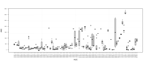
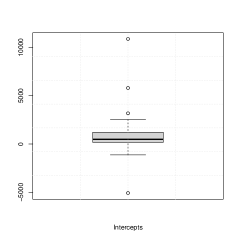
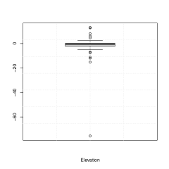
Figure 1: Boxplots displaying the distribution of ANC values by area (top panel) and the distribution of the estimated values of the intercept and the slope (bottom panel) obtained fitting a regression model area by area where the ANC is the response variable and the elevation is the covariate.

3 Notation and background

Consider $m$ small areas with the $i$th small area population consisting of $N_{i}$ units. Let $y_{ij}$ and ${\mathbf{x}}_{ij}$ denote the values of the study variable and a $p\times 1$ vector of known auxiliary variables for the $j$th unit of the $i$th small area, respectively, with $i=1,\dots,m,\,j=1,\dots,N_{i}.$ We are interested in estimating the small area means $\bar{Y}_{i}=N_{i}^{-1}\sum_{j=1}^{N_{i}}y_{ij}$ using a simple random sample $s$ of size $n$ drawn from the finite population covering all $m$ areas and $\bar{{\mathbf{X}}}_{i}=N_{i}^{-1}\sum_{j=1}^{N_{i}}{\mathbf{x}}_{ij}$, the vector $p\times 1$ of finite population means of the auxiliary variables for area $i$. In a typical small area estimation situation, $n_{i}$, sample size for area $i$, is not large enough to support the use of a direct estimator, the sample mean $\bar{y}_{i}=n_{i}^{-1}\sum_{j\in s_{i}}y_{ij},$ where $s_{i}$ denotes the part of the sample from the $i$th small area. Here $n=\sum_{i=1}^{m}n_{i}$.

Battese et al., (1988) considered the following nested error regression model for the finite population:

$$y_{ij}=\beta_{0}+{\mathbf{x}}_{ij}^{\prime}\boldsymbol{\beta}+\gamma_{i}+\epsilon_{ij},\;i=1,\dots,m;\;j=1,\dots,N_{i},$$ (1)

where $\beta_{0}$ and $\boldsymbol{\beta}$ are unknown fixed intercept and regression coefficients, respectively; $\gamma_{i}$ is a random effect for area $i$ that attempts to incorporate the leftover between area variations not captured by the auxiliary variables ${\mathbf{x}}_{ij}$; $\epsilon_{ij}$ is the sampling error for the $j$th observation in the $i$th area, which captures the leftover variations not accounted for the other components of the model. The area specific random effects $\gamma_{i}$ and the sampling errors $\epsilon_{ij}$ are all assumed to be independent with $\gamma_{i}\sim N(0,\sigma_{\gamma}^{2})$ and $\epsilon_{ij}\sim N(0,\sigma_{\varepsilon}^{2}),\;i=1,\dots,m;\;j=1,\dots,N_{i}$. The parameters $\boldsymbol{\delta}=(\sigma_{\gamma}^{2},\sigma_{\varepsilon}^{2})$ are referred to as the variance components of model (1).

Battese et al., (1988) argued that, under the assumed nested error model (1), the finite population mean $\bar{Y}_{i}$ can be well approximated by $\theta_{i}=\beta_{0}+\bar{\mathbf{X}}_{i}^{\prime}\boldsymbol{\beta}+\gamma_{i}$, for large $N_{i}$. Battese et al., (1988) proposed an empirical best linear unbiased predictor (EBLUP) for estimating $\theta_{i}$ given by

$$\hat{\theta}_{i}^{BHF}=\hat{\boldsymbol{\beta}}_{0}+\bar{\mathbf{X}}^{\prime}_{i}\hat{\boldsymbol{\beta}}+\hat{\gamma}_{i},$$ (2)

where $\hat{\boldsymbol{\beta}}_{0}$ and $\hat{\boldsymbol{\beta}}$ are weighted least square estimators of $\beta_{0}$ and $\boldsymbol{\beta},$ respectively; $\hat{\gamma}_{i}=(1-\hat{B}_{i})(\bar{y}_{i}-\hat{\boldsymbol{\beta}}_{0}-\bar{\mathbf{x}}_{i}^{\prime}\hat{\boldsymbol{\beta}})$ is the EBLUP of $\gamma_{i}$ with $\bar{{\mathbf{x}}}_{i}=n_{i}^{-1}\sum_{j\in s_{i}}{\mathbf{x}}_{ij},\;\hat{B}_{i}=\frac{\hat{\sigma}_{\epsilon}^{2}/n_{i}}{\hat{\sigma}_{\epsilon}^{2}/n_{i}+\hat{\sigma}_{\gamma}^{2}}$ and $\hat{\boldsymbol{\delta}}=(\hat{\sigma}_{\gamma}^{2},\hat{\sigma}_{\epsilon}^{2})$ is a consistent estimator of $\boldsymbol{\delta}=(\sigma_{\gamma}^{2},\sigma_{\epsilon}^{2})$ under model (1); see Battese et al., (1988) for details. The authors implicitly assumed non-informative sampling so that the same nested error model (1) holds for the sample.

The synthetic assumption of identical regression coefficients $\boldsymbol{\beta}$ and sampling variance $\sigma_{\epsilon}^{2}$ across all small areas to be combined may be unrealistic when the number of small areas $m$ is large. The synthetic assumption on $\boldsymbol{\beta}$ can be relaxed if we replace $\boldsymbol{\beta}$ in (1) by random area specific regression $\boldsymbol{\beta}_{i}$, $i=1,\dots,m$, generated from a common model, e.g., a common $p$-dimensional multivariate normal model with common mean vector and variance-covariance matrix. This additional assumption for random effects is necessary to reduce the number of unknown parameters; see Prasad and Rao, (1990). Rao and Molina, (2015, p. 173) relaxed the homogeneity assumption of the individual errors by replacing $\sigma_{\epsilon}^{2}$ by $k_{ij}\sigma_{\epsilon}^{2}$, where $k_{ij}>0$ is a known auxiliary variable. However, identifying $k_{ij}$ in a real-life data analysis may be hard and between area variability may not be fully explained by $k_{ij}$. In the next section, we propose an alternative solution.

4 Model and method

We propose the following extension of the nested error regression model:

$$y_{ij}=\beta_{0}+{\mathbf{x}}_{ij}^{\prime}\boldsymbol{\beta}_{i}+\gamma_{i}+\epsilon_{ij},\;i=1,\dots,m;\;j=1,\dots,N_{i},$$ (3)

where $\boldsymbol{\beta}_{i}$ is a $p\times 1$ vector of fixed unknown regression coefficients for area $i$; $\gamma_{i}$ and $\epsilon_{ij}$ are all independent with $\gamma_{i}\sim N(0,h_{i}\sigma_{\gamma}^{2})$ and $\varepsilon_{ij}\sim N(0,k_{ij}\sigma_{\varepsilon i}^{2})$, with $h_{i}$ and $k_{ij}$ are known auxiliary variables at area and individual levels, respectively. This model can be called a nested error regression with high dimensional parameter. Battese et al., (1988) considered a special case of model (3) with $h_{i}=1$, $k_{ij}=1$, $\boldsymbol{\beta}_{i}=\boldsymbol{\beta}$ and $\sigma_{\varepsilon i}^{2}=\sigma_{\varepsilon}^{2}$; $i=1,\dots,m;j=1,\dots,N_{i}$.

Under model (3) and non-informative sample design, the best predictor (BP) of $\theta_{i}=\beta_{0}+\bar{\mathbf{X}}_{i}^{\prime}\boldsymbol{\beta}_{i}+\gamma_{i}$ is given by

$$\hat{\theta}_{i}^{BP}\equiv\hat{\theta}_{i}(\boldsymbol{\phi}_{i}) = \beta_{0}+\bar{{\mathbf{X}}}^{\prime}_{i}\boldsymbol{\beta}_{i}+(1-B_{i})(\bar{y}_{i}-\beta_{0}-{\bar{{\mathbf{x}}}}_{i}^{\prime}\boldsymbol{\beta}_{i})$$ (4)

$$= (\bar{{\mathbf{X}}}_{i}-\bar{{\mathbf{x}}}_{i})^{\prime}\boldsymbol{\beta}_{i}+\left\{B_{i}(\beta_{0}+\bar{{\mathbf{x}}}_{i}^{\prime}\boldsymbol{\beta}_{i})+(1-B_{i})\bar{y}_{i}\right\},$$

where $B_{i}=\frac{{\sigma}_{\epsilon i}^{2}/n_{i}}{{\sigma}_{\epsilon i}^{2}/n_{i}+\sigma_{\gamma}^{2}}$ and $\boldsymbol{\phi}_{i}=(\beta_{0},\boldsymbol{\beta}_{i},\sigma_{\gamma}^{2},\sigma_{\varepsilon i}^{2})^{\prime}$.

Under simple random sampling, $\hat{\theta}_{i}^{BP}$ is design-consistent for $\theta_{i}$ because, as $n_{i}$ increases, $\hat{\theta}_{i}^{BP}$ approaches to the design-consistent estimator $\bar{y}_{i}$ since $B_{i}\rightarrow 0$ and $\bar{{\mathbf{x}}}_{i}$ is design-consistent for $\bar{{\mathbf{X}}}_{i}$. An empirical best predictor (EBP) of $\theta_{i}$ can be written as $\hat{\theta}_{i}^{EBP}\equiv\hat{\theta}_{i}(\hat{\boldsymbol{\phi}}_{i}),$ where $\hat{\boldsymbol{\phi}}_{i}$ is a consistent estimator of $\boldsymbol{\phi}_{i}$ under the assumed model (3) as $m$ tends to $\infty$. A BP of $\bar{Y}_{i}$ that uses the sampling fraction $f_{i}=n_{i}/N_{i}$ is given by $\hat{\bar{Y}}_{i}^{BP}=f_{i}\bar{y}_{i}+(1-f_{i})\hat{\theta}_{i}^{BP}$. We note that $\hat{\theta}_{i}^{BP}$ and $\hat{\bar{Y}}_{i}^{BP}$ are both design-consistent even when $f_{i}$ is a fixed negligible constant.

5 Estimation of the vector of the parameters $\boldsymbol{\phi}_{i}=(\beta_{0},\boldsymbol{\beta}_{i},\sigma_{\gamma}^{2},\sigma_{\varepsilon i}^{2})^{\prime}$

We begin the section by first describing the maximum likelihood method for estimating $\boldsymbol{\phi}_{i}$, $i=1,\dots,m$. For model (3), the log-likelihood function has the expression

$$\ell(\boldsymbol{\phi}) = constant-\frac{1}{2}\sum_{i=1}^{m}\left[n_{i}\log{\sigma_{\epsilon i}^{2}}+\log{\left[\frac{\sigma_{\epsilon i}^{2}+n_{i}\sigma_{\gamma}^{2}}{\sigma_{\epsilon i}^{2}}\right]}\right.$$ (5)

$$\left.+\frac{1}{\sigma_{\epsilon i}^{2}}\left\{\sum_{j=1}^{n_{i}}(y_{ij}-\beta_{0}-{\mathbf{x}}_{ij}^{\prime}\boldsymbol{\beta}_{i})^{2}-\frac{\sigma_{\gamma}^{2}}{\sigma_{\epsilon i}^{2}+n_{i}\sigma_{\gamma}^{2}}(n_{i}\bar{y}_{i}-n_{i}\beta_{0}-n_{i}\bar{{\mathbf{x}}}_{i}^{\prime}\boldsymbol{\beta}_{i})^{2}\right\}\right],$$

where the constant does not depend on the parameters, $\boldsymbol{\phi}=(\boldsymbol{\phi}_{1},\dots,\boldsymbol{\phi}_{m})$. The maximum likelihood estimators (MLEs) of the parameters are obtained by differentiating the $\ell(\boldsymbol{\phi})$ with respect to $\beta_{0},\boldsymbol{\beta}_{i},\sigma_{\gamma}^{2},\sigma_{\varepsilon i}^{2}$ and solving the system of estimating equations sets out equal to zero. In particular, given the variance components, the MLE of the regression coefficients for area $i$ are:

$$\hat{\beta}_{0}=\left(\sum_{i=1}^{m}\sigma_{\epsilon i}^{-2}n_{i}B_{i}\right)^{-1}\left(\sum_{i=1}^{m}\sigma_{\epsilon i}^{-2}n_{i}B_{i}(\bar{y}_{i}-\bar{{\mathbf{x}}}_{i}^{\prime}\boldsymbol{\beta}_{i})\right),$$ (6)

$$\hat{\boldsymbol{\beta}}_{i}=\left(\sum_{j=1}^{n_{i}}{\mathbf{x}}_{ij}{\mathbf{x}}_{ij}^{\prime}-n_{i}(1-B_{i})\bar{{\mathbf{x}}}_{i}\bar{{\mathbf{x}}}_{i}^{\prime}\right)^{-1}\left(\sum_{j=1}^{n_{i}}{\mathbf{x}}_{ij}(y_{ij}-\beta_{0})-n_{i}(1-B_{i})\bar{{\mathbf{x}}}_{i}(\bar{y}_{i}-\beta_{0})\right),$$ (7)

and, given the regression coefficients, the MLE of the sampling variance for area $i$ is:

$$\hat{\sigma}_{\epsilon i}^{2}=\frac{1}{n_{i}}\left\{\sum_{j=1}^{n_{i}}(y_{ij}-\beta_{0}-{\mathbf{x}}_{ij}^{\prime}\boldsymbol{\beta}_{i})^{2}-n_{i}(1-B_{i})(\bar{y}_{i}-\beta_{0}-\bar{{\mathbf{x}}}_{i}^{\prime}\boldsymbol{\beta}_{i})^{2}\right\}.$$ (8)

Neyman and Scott, (1948) gave an example which shows that, when the number of nuisance parameters increases with the at the same rate as the sample size, the MLEs may not be consistent. Another example was given by Jiang and Nguyen, (2012). The latter authors considered a heteroscedastic NER model with area-specific error variance, and noted that the MLE of the area-specific error variance is inconsistent.

As in the Neyman-Scott and Jiang and Nguyen problems, in our proposed model the number of unknown parameters is proportional to the sample size, if the area sample sizes ($n_{i}$) are bounded, which is typically the case in small area estimation problems (Jiang and Nguyen,, 2012). Note that consistent estimators of regression coefficients ($\beta_{0},\boldsymbol{\beta}_{i}$) and variance components ($\sigma_{\gamma}^{2},\sigma_{\varepsilon i}^{2}$) are all that is needed to justify the use of the proposed EBP as a point predictor.

In this paper, a generalized estimating equation (GEE) approach is used to estimate the parameters of model (3); this method allows to borrow strength across areas when estimating each area specific vector of parameters obtaining consistent estimators of the area specific slope parameters ($\boldsymbol{\beta}_{i}$) and the area specific sampling variance ($\sigma_{\varepsilon i}^{2}$). Because of more flexibility in estimating the model parameters than that of the maximum likelihood, our estimating equation method is likely to have an edge over the maximum likelihood in terms of the predictive power, which is important in the small area estimation context. For known area specific tuning parameter $\tau_{i}$, our estimating equation method yields consistent estimators of the model parameters, unlike the maximum likelihood method.

We now describe the algorithm based on GEE approach for estimating $\boldsymbol{\phi}_{i}$, $i=1,\dots,m$, in the following steps.

• At each iteration $t=1,2,\dots$, define the following $n_{l}\times n_{l}$ matrix:

  $${\mathbf{V}}_{l;i}^{(t-1)}=h_{l}\sigma_{\gamma}^{2(t-1)}{\mathbf{1}}_{n_{l}}{\mathbf{1}}_{n_{l}}^{\prime}+\sigma_{\epsilon i}^{2(t-1)}{\mathbf{K}}_{l},$$

  where ${\mathbf{1}}_{n_{l}}$ denotes a vector of ones of length $n_{l}$ and ${\mathbf{K}}_{l}=\mbox{diag}(k_{l1},\dots,k_{ln_{l}})$ is a $n_{l}\times n_{l}$ diagonal matrix, $l=1,\dots,m$. Let ${\mathbf{U}}_{l;i}^{(t-1)}$ be a $n_{l}\times n_{l}$ diagonal matrix with diagonal elements equal to those of ${\mathbf{V}}_{l;i}^{(t-1)},l=1,\dots,m.$ Set ${\beta}_{0}=\sum_{i=1}^{m}{\alpha}_{0i}/m$ and start with initial values, say $\{\alpha_{0i}^{(0)},\boldsymbol{\beta}_{i}^{(0)},\sigma_{\gamma}^{2(0)},\sigma_{\epsilon i}^{2(0)},\;i=1,\dots,m\}$, for $\{\alpha_{0i},\boldsymbol{\beta}_{i},\sigma_{\gamma}^{2},\sigma_{\epsilon i}^{2},\;i=1,\dots,m\}$.

• For $t=1,2,\dots$ define ${\mathbf{r}}_{l;i}^{(t)}=({\mathbf{U}}_{l;i}^{(t-1)})^{-1/2}({\mathbf{y}}_{l}-{\color[rgb]{0,0,0}\alpha_{0i}^{(t)}{\mathbf{1}}_{n_{l}}-{\mathbf{X}}_{l}\boldsymbol{\beta}_{i}^{(t)}})$, where ${\mathbf{y}}_{l}$ is a $n_{l}\times 1$ vector of the response variable and ${\mathbf{X}}_{l}$ denotes a matrix $n_{l}\times p$ of individual level covariates of the sampling units in area $l$. Obtain $(\alpha_{0i}^{(t)},\boldsymbol{\beta}_{i}^{(t)})$ by solving the following system of estimating equations for $(\alpha_{0i},\boldsymbol{\beta}_{i})$:

  $$\sum_{l=1}^{m}\left[{\mathbf{X}}_{l(p+1)}({\mathbf{V}}_{l;i}^{(t-1)})^{-1}({\mathbf{U}}_{l;i}^{(t-1)})^{1/2}\psi_{i}({\mathbf{r}}_{l;i}^{(t)})\right]={\mathbf{0}},\leavevmode\nobreak\ \leavevmode\nobreak\ i=1,\dots,m,$$ (9)

  where $\psi_{i}({\mathbf{r}}_{l;i}^{(t)})$ is a $n_{l}\times 1$ vector obtained from the vector of residuals ${\mathbf{r}}_{l;i}^{(t)}$ with its $j$th component, say $r_{lj;i}^{(t)}$, replaced by $\psi_{i}(r_{lj;i}^{(t)}),$ a chosen known function of $r_{lj;i}^{(t)}.$ Here ${\mathbf{X}}_{l(p+1)}$ denotes a matrix of dimension $n_{l}\times(p+1)$ containing the covariates of the sampling units of area $l$ including the intercept. The solution $(\alpha_{0i}^{(t)},\boldsymbol{\beta}_{i}^{(t)})$ for $i=1,\dots,m$ can be obtained using an iteratively re-weighted least squares algorithm or the Newton-Raphson algorithm.

  
  

  Remark 1: In this section, we assume that the function $\psi_{i}(r)$ is completely specified. For example,

  $$\psi_{i}(r)=2\psi(r)\left[\tau_{i}I(r>0)+(1-\tau_{i})I(r\leq 0)\right],\;-\infty<r<\infty,$$

  where $\psi(r)$ is a known monotone non-decreasing function with $\psi(-\infty)<\psi(0)<\psi(\infty)$, $\tau_{i}\in\Omega=(0,1)$ known, and $r$ is a re-scaled residual. Note that the choice $\tau_{i}=0.5$ would lead to the standard weighted least square estimator of the regression coefficient vector. The case for unknown $\tau_{i}$ will be discussed in the next section. Two popular choices of $\psi(r)$ are $\psi(r)=\mbox{sign}(r)$ and $\psi(r)=r$. In small area estimation context, Chambers and Tzavidis, (2006) assume that $\psi(r)$ is the Huber influence function with tuning constant $c>0$ (Huber,, 1981). The authors used $c=1.345$ in producing their M-quantile-based (MQ) estimators of the small area means. An alternative to the Huber function could be the Tukey’s bisquare function. In the analysis of repeated measures, Higgins, (1993) noted that if one uses Tukey’s bisquare function in robustifying log-likelihood, this function appears in the corresponding estimating equations.

  
  

  Remark 2: Note that estimates of the components $\boldsymbol{\beta}_{i}$ and $\sigma_{\varepsilon i}^{2}$ in $\boldsymbol{\phi}_{i}$ are subject to high variability if we use data only from area $i$ to estimate these area specific fixed parameters because of small area specific sample sizes. Here, for known $\tau_{i}$, we overcome this problem using an algorithm that uses data from all areas.

• Define $\tilde{{\mathbf{r}}}_{l;i}^{(t)}=(\tilde{{\mathbf{U}}}_{l;i}^{(t-1)})^{-1/2}({\mathbf{y}}_{l}-\alpha_{0i}^{(t)}{\mathbf{1}}_{n_{l}}-{\mathbf{X}}_{l}\boldsymbol{\beta}_{i}^{(t)})$ with $\tilde{{\mathbf{U}}}_{l;i}^{(t-1)}$ represents a $n_{l}\times n_{l}$ diagonal matrix with diagonal elements equal to those of $\tilde{{\mathbf{V}}}_{l;i}^{(t-1)}=h_{l}\sigma_{\gamma}^{2(t-1)}{\mathbf{1}}_{n_{l}}{\mathbf{1}}_{n_{l}}^{\prime}+\sigma_{\epsilon i}^{2(t)}{\mathbf{K}}_{l}$. Obtain $\{\sigma_{\epsilon i}^{2(t)},\;i=1,\dots,m\}$ as a solution of the following system of estimating equations:

  $$\sum_{l=1}^{m}\left[\psi_{i}(\tilde{{\mathbf{r}}}_{l;i}^{(t)})^{\prime}(\tilde{{\mathbf{U}}}_{l;i}^{(t-1)})^{1/2}(\tilde{{\mathbf{V}}}_{l;i}^{(t-1)})^{-1}\frac{\partial{\mathbf{V}}_{i;i}}{\partial\sigma_{\epsilon i}^{2}}|_{\sigma_{\gamma}^{2}=\sigma_{\gamma}^{2(t-1)}}(\tilde{{\mathbf{V}}}_{l;i}^{(t-1)})^{-1}(\tilde{{\mathbf{U}}}_{l;i}^{(t-1)})^{1/2}\psi_{i}(\tilde{{\mathbf{r}}}_{l;i}^{(t)})\right.$$

  $$-\left.w_{i}\;\mbox{tr}\left\{(\tilde{{\mathbf{V}}}_{l;i}^{(t-1)})^{-1}\frac{\partial{\mathbf{V}}_{i;i}}{\partial\sigma_{\epsilon i}^{2}}|_{\sigma_{\gamma}^{2}=\sigma_{\gamma}^{2(t-1)}}(\tilde{{\mathbf{V}}}_{l;i}^{(t-1)})^{-1}\frac{\partial{\mathbf{V}}_{i;i}}{\partial\sigma_{\epsilon i}^{2}}|_{\sigma_{\gamma}^{2}=\sigma_{\gamma}^{2(t-1)}}\right\}\right]=0$$ (10)

  where $i=1,\dots,m$, ${{\mathbf{V}}}_{i;i}=h_{i}\sigma_{\gamma}^{2}{\mathbf{1}}_{n_{i}}{\mathbf{1}}_{n_{i}}^{\prime}+\sigma_{\epsilon i}^{2}{\mathbf{K}}_{i}$ and $w_{i}=E[\psi_{i}^{2}(u)],$ with $u\sim N(0,1)$.

• After Steps 2 and 3 the estimates of $\boldsymbol{\beta}_{i}$ and $\sigma_{\epsilon_{i}}^{2}$ are obtained for each small area. Then an estimate of $\beta_{0}$ at iteration $t$ is obtained as ${\beta}_{0}^{(t)}=\sum_{i=1}^{m}{\alpha}_{0i}^{(t)}/m$. An alternative method for the estimation of $\beta_{0}$ can constrain the intercept value to be equal in the estimating equations (9) for all small areas. We have tested both the estimation procedures in the simulation experiments and we have not found difference in the estimates. For this reason we propose to adopt the first and much simpler method to estimate $\beta_{0}$. For the estimation of $\sigma_{\gamma}^{2}$ compute ${\mathbf{r}}^{\star(t)}=({\mathbf{r}}_{1}^{\star(t)\prime},\dots,{\mathbf{r}}_{i}^{\star(t)\prime},\dots,{\mathbf{r}}_{m}^{\star(t)\prime})^{\prime}$, where ${\mathbf{r}}_{i}^{\star(t)}={\mathbf{y}}_{i}-{\beta}_{0}^{(t)}{\mathbf{1}}_{n_{i}}-{\mathbf{X}}_{i}{\boldsymbol{\beta}}_{i}^{(t)}$. Obtain $\sigma_{\gamma}^{2(t)}$ as a solution of the following estimating equation:

  $$\psi(({\mathbf{A}}^{(t)})^{-1/2}{\mathbf{r}}^{\star(t)})^{\prime}({\mathbf{A}}^{(t)})^{1/2}({\mathbf{G}}^{(t)})^{-1}{\mathbf{Z}}{\mathbf{Z}}^{\prime}({\mathbf{G}}^{(t)})^{-1}({\mathbf{A}}^{(t)})^{1/2}\psi(({\mathbf{A}}^{(t)})^{-1/2}{\mathbf{r}}^{\star(t)})$$

  $$-w^{\star}\;\mbox{tr}\left(({\mathbf{G}}^{(t)})^{-1}{\mathbf{Z}}{\mathbf{Z}}^{\prime}({\mathbf{G}}^{(t)})^{-1}{\mathbf{Z}}{\mathbf{Z}}^{\prime}\right)=0,$$ (11)

  where ${\mathbf{Z}}=\mbox{diag}({\mathbf{1}}_{n_{i}},\leavevmode\nobreak\ i=1,\cdots,m)$ is the incidence matrix of dimension $n\times m$; $w^{\star}=E[\psi^{2}(u)],$ with $u\sim N(0,1)$; ${\mathbf{G}}^{(t)}=\sigma_{\gamma}^{2(t)}{\mathbf{Z}}{\mathbf{H}}{\mathbf{Z}}^{\prime}+{\mathbf{R}}^{(t)}$ of order $n\times n$ with ${\mathbf{H}}$ is a diagonal matrix $m\times m$ with diagonal elements equal to $(h_{1},\dots,h_{i},\dots,h_{m})$ and ${\mathbf{R}}^{(t)}$ is a diagonal matrix $n\times n$ with diagonal elements equal to $(\underbrace{k_{11}\sigma_{\epsilon 1}^{2(t)},\dots,k_{1n_{1}}\sigma_{\epsilon 1}^{2(t)}}_{n_{1}},\dots,\underbrace{k_{i1}\sigma_{\epsilon i}^{2(t)},\dots,k_{in_{i}}\sigma_{\epsilon i}^{2(t)}}_{n_{i}},\dots,\underbrace{k_{m1}\sigma_{\epsilon m}^{2(t)},\dots,k_{mn_{m}}\sigma_{\epsilon m}^{2(t)}}_{n_{m}})$; ${\mathbf{A}}^{(t)}$ is a diagonal matrix with diagonal elements $a_{ij}$ equal to the diagonal elements of the covariance matrix ${\mathbf{G}}^{(t)}$. This estimating equation is proposed following the lines of maximum likelihood proposal II due to Richardson and Welsh, (1995).

• Repeat Steps 2-4 until convergence to obtain the estimated vector $\hat{\boldsymbol{\phi}}_{i}$. Convergence is achieved when the difference between the estimated model parameters obtained from two successive iterations is less than a small pre-specified value.

Like any other iterative algorithm, the proposed procedure requires initial values for the parameters. As a result, using well-defined starting values for the fixed and variance parameters is advisable for reducing the computational time. Here we suggest to employ a deterministic strategy for initialisation, based on considering the estimates of regression coefficients and variance components obtained by the standard linear mixed model as starting points for all areas. Obviously, this strategy can be substantially improved by adopting a multi-start random initialisation, as the one we have used in the analysis of real data examples (see Section 8). However, this strategy may significantly increase the global computational burden and, for this reason, it is not employed in this large scale simulation study.

For large $m$, under appropriate regularity conditions on the model and known $\psi_{i}$ function, consistency of the estimator $\hat{\boldsymbol{\phi}}_{i}$ of $\boldsymbol{\phi}_{i}$ can be established in a straightforward way, using Theorem 3.6 of Jiang, (2017, pp. 100-101) or Theorem 4.1 of Jiang et al., (2002). Assuming that the joint distribution of the observations $({\mathbf{y}}_{l})_{1\leqslant l\leqslant m}$ (vector-valued) depends on $\boldsymbol{\phi}_{i}$, equations (9), (Step 3) and (Step 4) can be written as:

$$F_{i}(\boldsymbol{\phi}_{i})=\sum_{l=1}^{m}f_{l}(\boldsymbol{\phi}_{i},{\mathbf{y}}_{l})+h(\boldsymbol{\phi}_{i}),$$ (12)

where $f_{l}(\boldsymbol{\phi}_{i},{\mathbf{y}}_{l})=(f_{l,k}(\boldsymbol{\phi}_{i},{\mathbf{y}}_{l}))_{1\leqslant k\leqslant(p+3)}$ are vector-valued functions such that $E[f_{l}(\boldsymbol{\phi}_{0i},{\mathbf{y}}_{l})]=0$, $l=1,\dots,m$, $\boldsymbol{\phi}_{0i}$ is the true vector of parameters and $h(\boldsymbol{\phi}_{i})$ is a vector-valued which may depend on the joint distribution of $({\mathbf{y}}_{l})_{1\leqslant l\leqslant m}$. As pointed out by Jiang et al., (2002) these equations maybe regarded as M-estimating equations and the estimators as M-estimators. Then we can state as it follows:

Preposition 1

Suppose that regularity conditions (i)-(viii) (Jiang et al.,, 2002; Chambers et al.,, 2014) given in Appendix hold and $\psi_{i}$ functions are completely specified. Then the resulting vector of estimators $\hat{\boldsymbol{\phi}}_{i}$ is consistent.

Proof This result is a modified version of that obtained by Jiang et al., (2002) and Jiang, (2017).

Substituting $\hat{\boldsymbol{\phi}}_{i}$ for $\boldsymbol{\phi}_{i}$ in equation (4), we get empirical best predictor $\hat{\theta}_{i}^{EBP}\equiv\hat{\theta}_{i}(\hat{\boldsymbol{\phi}}_{i})$ of $\theta_{i}$. We now present asymptotic behavior of the relative savings loss (RSL) of EBP over any direct estimator of $\theta_{i}$. The concept of relative savings loss was introduced by Efron and Morris (1973). In terms of RSL, the following result shows that $\hat{\theta}_{i}^{EBP}$ is closer to the optimal best predictor, $\hat{\theta}_{i}^{BP}$, under model (3), than any direct or synthetic estimator $\tilde{\theta}_{i}$.

Preposition 2

Under the model (3) and mild regularity conditions,

$$RSL(\hat{\theta}_{i}^{EBP},\tilde{\theta}_{i})=\frac{MSE(\hat{\theta}_{i}^{EBP})-MSE(\hat{\theta}_{i}^{BP})}{MSE(\tilde{\theta}_{i})-MSE(\hat{\theta}_{i}^{BP})}\longrightarrow 0,\;\mbox{as}\;m\rightarrow\infty,$$

where MSE is the mean squared error under model (3).

Proof An outline of the proof is as it follows. Using the definition of the best predictor, first note that

$$MSE(\hat{\theta}_{i}^{EBP})-MSE(\hat{\theta}_{i}^{BP})=E(\hat{\theta}_{i}^{EBP}-\hat{\theta}_{i}^{BP})^{2}.$$

Under model (3), regularity conditions and some algebra, we can show that

$$\hat{\theta}_{i}^{EBP}-\hat{\theta}_{i}^{BP}\stackrel{{\scriptstyle P}}{{\longrightarrow}}0,\;\mbox{as}\;m\rightarrow\infty.$$

Moreover, the uniform integrability of $(\hat{\theta}_{i}^{EBP}-\hat{\theta}_{i}^{BP})^{2}$ in $m$ follows since

$$\mbox{sup}_{m\geq 1}E(\hat{\theta}_{i}^{EBP}-\hat{\theta}_{i}^{BP})^{2+\delta}<\infty,$$

for any $\delta>0,$ under model (3), regularity conditions and considerable algebra. Thus,

$$MSE(\hat{\theta}_{i}^{EBP})-MSE(\hat{\theta}_{i}^{BP})\longrightarrow 0\;\mbox{as}\;m\rightarrow\infty.$$

The result now follows because

$$\mbox{inf}_{m\geq 1}\left[MSE(\tilde{\theta}_{i})-MSE(\hat{\theta}_{i}^{BP})\right]=\mbox{inf}_{m\geq 1}E(\hat{\theta}_{i}^{EBP}-\hat{\theta}_{i}^{BP})^{2}>0.$$

The proof is technical and goes along the lines of Ghosh and Lahiri, (1987). The details are left out to save space, but are available from the authors upon request.

Remark 3: Following Chambers and Tzavidis, (2006), one can obtain an MQ estimator of $\theta_{i}$ under model (3) when $\tau_{i}$ is known. We note that such an estimator would be a synthetic estimator of $\theta_{i}$ and so will be less efficient in terms of the above RSL criterion. Moreover, such an estimator of $\theta_{i}$ will not be design-consistent as the area specific sample size grows.

Remark 4: Following Tzavidis et al., (2010) (see also equation (18) in Fabrizi et al.,, 2014), one can adjust the MQ estimator in Remark 3 for design-consistency. Such an estimator would then be a direct estimator and so would be inferior to the EBP in terms of RSL.

5.1 Estimation of $\tau_{i}$

We now present a data-driven method to estimate $\tau_{i}$. For a fine grid $\tau\in\Omega,$ we fit a collection of regression models:

$$y_{ij}=\beta_{0\tau}+{\mathbf{x}}_{ij}^{\prime}\boldsymbol{\beta}_{\tau}+e_{ij},\;i=1,\dots,m;\;j=1,\dots,n_{i},$$

using the standard quantile or M-quantile methods (Koenker,, 2005; Breckling and Chambers,, 1988), where $\beta_{0\tau}$ and $\boldsymbol{\beta}_{\tau}$ are fixed intercept and regression coefficients, respectively, and $e_{ij}$’s are standard random errors.

For each observation $y_{ij}$, we find the fitted line with minimum prediction error defined as the difference between $y_{ij}$ and the predicted value by the fitted regression at ${\mathbf{x}}_{ij}$. Let $\hat{\tau}_{ij}$ denote the value of $\tau$ in the grid for this best line. Chambers and Tzavidis, (2006) called $\hat{\tau}_{ij}$ estimated M-quantile coefficients. Their variability reflects variability at the unit level. If clustering exists, population units in the same cluster (or small area) will have similar M-quantile coefficients and these will be different from those of units that belong to other clusters (or areas). Provided that there are sample observations in area $i$, and a non-informative sampling method has been used to obtain them, an estimate of the area-$i$-specific M-quantile coefficient is the sample average of the estimated M-quantile coefficients for that area, $\bar{\hat{\tau}}_{i}=n_{i}^{-1}\sum_{j\in s_{i}}\hat{\tau}_{ij}$. Since $n_{i}$ is typically small, $\bar{\hat{\tau}}_{i}$ is likely to be unstable. We propose the following empirical linear best (ELB) predictor of $\tau_{i}$ , which improves on $\bar{\hat{\tau}}_{i}$ because it uses data from all areas using the following model:

1. $E[\hat{\tau}_{ij}|\tau_{i}]=\tau_{i}$, $V[\hat{\tau}_{ij}|\tau_{i}]=\nu^{2}$,

2. $E[\tau_{i}]=\mu$, $V[\tau_{i}]=\eta^{2}$.

Assuming $E[\tau_{i}|\hat{\boldsymbol{\tau}}]=\alpha+\beta\bar{\hat{\tau}}_{i}$, the linear best (LB) predictor of $\tau_{i}$ can be written as

$$\hat{\tau}_{i}^{LB}=(1-B_{i})\bar{\hat{\tau}}_{i}+B_{i}\mu,$$ (13)

where $B_{i}=\frac{\nu^{2}/n_{i}}{\nu^{2}/n_{i}+\eta^{2}}$. Substituting $\mu$, $\eta^{2}$ and $\nu^{2}$ by their consistent estimators $\hat{\mu}$, $\hat{\eta}^{2}$ and $\hat{\nu}^{2}$, we obtain the following empirical linear best (ELB) predictor:

$$\hat{\tau}_{i}^{ELB}=(1-\hat{B}_{i})\bar{\hat{\tau}}_{i}+\hat{B}_{i}\hat{\mu},$$ (14)

where $\hat{B}_{i}=\frac{\hat{\nu}^{2}/n_{i}}{\hat{\nu}^{2}/n_{i}+\hat{\eta}^{2}}$. We refer to Ghosh and Meeden, (1997) for a detailed theory on empirical linear best estimator in the context of finite population sampling.

The concept of the proposed data driven estimation of $\tau_{i}$ for the specific choice of $\psi$ function is grounded on the basis of increasing predictive power of our proposed method. When $n_{i}$’s are small, resulting estimators of the model parameters $\boldsymbol{\phi}$ are not consistent, like the MLE. In order to achieve consistency, we need large $n_{i}$ at the minimum. For the regression context, Bianchi and Salvati, (2015) considered consistency of similar tuning parameter estimators. In this paper, since $n_{i}$’s are assumed to be small, we evaluate the performance of our proposed methodology through extensive simulation and demonstrate the utility of our method over existing rival methods.

6 Uncertainty measures

For known $\tau_{i}$, our estimators of uncertainty measures (not necessarily MSE) tend to the true corresponding uncertainty measures in probability as $m$ tends to infinity, under certain regularity conditions, including the regularity conditions of Proposition 1. For unknown $\tau_{i}$, such a convergence does not hold unless possibly within area sample sizes $n_{i}$ are large. We do not pursue this research here because our focus is on bounded $n_{i}$. As stated in the concluding remarks, investigation of such asymptotic properties could be an interesting topic for future research.

In this section, we discuss the estimation of a general class of uncertainty measures for a small area estimator, say $\hat{\theta}_{i}$, not necessarily an empirical best predictor. An uncertainty measure in this general class is denoted by $f(\mbox{E}[d(\hat{\theta}_{i},\theta_{i})])$, where $f(\cdot)$ denotes a known, possibly non-linear, function, $d(\hat{\theta}_{i},\theta_{i})$ is a known distance measure between $\hat{\theta}_{i}$ and $\theta_{i}$, and $E$ is the expectation with respect to the assumed model. Examples of such uncertainty measures include commonly used root mean squared error (RMSE) and relative root mean squared error (RRMSE) defined as

$$\mbox{RMSE}[\hat{\theta}_{i}]=\sqrt{\mbox{MSE}[\hat{\theta}_{i}]},$$ (15)

where $\mbox{MSE}[\hat{\theta}_{i}]=E[(\hat{\theta}_{i}-\theta_{i})^{2}]$, and

$$\mbox{RRMSE}[\hat{\theta}_{i}]=\frac{\mbox{RMSE}[\hat{\theta}_{i}]}{E[\hat{\theta}_{i}]},$$ (16)

respectively. As noted in the introduction, a customary estimator of $RMSE$ is a plug-in estimator $\sqrt{\widehat{\mbox{MSE}}}$, where $\widehat{\mbox{MSE}}$ is a second-order unbiased estimator of MSE. But, a function of an second-order unbiased estimator of MSE does not necessarily yield a second-order unbiased estimator of the corresponding function of MSE.

We propose a different approach that could potentially justify the use of a much simpler estimator of $f(\mbox{E}[d(\hat{\theta}_{i},\theta_{i})])$. To this end, we propose a more flexible modeling that allows us to combine a large number of small areas so that it suffices to use a simpler probabilistic convergence criterion. For example, unlike the traditional nested error regression model, we assume that regression coefficients and variance components in the nested error regression model vary across small areas - model (3). This milder model assumption allows us to include more small areas to be combined than the corresponding traditional nested error regression model and thereby making the proposed probabilistic convergence criterion more reasonable.

In some cases, it may be possible to apply an analytical method to produce a reasonable estimator of $f(\mbox{E}[d(\hat{\theta}_{i},\theta_{i})])$. For example, when $\tau_{i}$ is known, an estimator of RMSE for EBP, under the assumed model (3), is given by $\sqrt{g_{1i}(\hat{\boldsymbol{\phi}}_{i})}$, where

$$g_{1i}(\boldsymbol{\phi}_{i})=\frac{\sigma_{\gamma}^{2}\sigma_{\epsilon i}^{2}/n_{i}}{\sigma_{\gamma}^{2}+\sigma_{\epsilon i}^{2}/n_{i}},$$ (17)

and $\hat{\boldsymbol{\phi}}_{i}$ is a consistent estimator of $\boldsymbol{\phi}_{i}$, for large $m$. Note that a new derivation for such an analytical estimator of $f(\mbox{E}[d(\hat{\theta}_{i},\theta_{i})])$ would be necessary as we change the model, the estimator $\hat{\theta}_{i}$, the distance function $d$ or the $f$ function. This makes such analytical method unattractive to analysts.

We now propose a simple parametric bootstrap method that can be applied to produce a reasonable estimator of $f(\mbox{E}[d(\hat{\theta}_{i},\theta_{i})])$. First, note that the joint distribution $\{(\theta_{i},y_{ij}),\;i=1,\dots,m;\;j=1,\dots,n_{i}\}$ is known except possibly for the model parameters $\boldsymbol{\phi}_{i}=(\beta_{0},\boldsymbol{\beta}_{i},\sigma_{\gamma}^{2},\sigma_{\varepsilon i}^{2})$. Thus, $f(\mbox{E}[d(\hat{\theta}_{i},\theta_{i})])\equiv a_{i}(\boldsymbol{\phi}_{i})$ is a function of $\boldsymbol{\phi}_{i}$.

The proposed parametric bootstrap procedure steps are described below:

• Given $\boldsymbol{\phi}_{i}$, generate $R$ parametric bootstrap replicates $\{y_{ij}^{(r)},i=1,\dots,m;j=1,\dots,n_{i},r=1,\dots,R\}$ using the following model:

  $$y_{ij}^{(r)}=\beta_{0}+{\mathbf{x}}_{ij}^{\prime}\boldsymbol{\beta}_{i}+\gamma_{i}^{(r)}+\epsilon_{ij}^{(r)},$$

  where $\gamma_{i}^{(r)}|\sigma_{\gamma}^{2}\sim N(0,h_{i}{\sigma}_{\gamma}^{2})$ and $\epsilon_{ij}^{(r)}|\sigma_{\varepsilon i}^{2}\sim N(0,k_{ij}\sigma_{\varepsilon i}^{2})$ are all independently distributed, $i=1,\dots,m;\;j=1,\dots,n_{i}$.

• For each replication $r$, compute the simulated parameter of interest: $\theta_{i}^{(r)}=\beta_{0}+\bar{\mathbf{X}}^{\prime}_{i}\boldsymbol{\beta}_{i}+\gamma_{i}^{(r)},\;r=1,\dots,R$.

• For each replication $r$, compute $\hat{\boldsymbol{\phi}}_{i}^{(r)}$ using the estimation algorithm described in Section 5 and compute $\hat{\theta}_{i}^{(r)}$, which may depend on $\hat{\boldsymbol{\phi}}_{i}^{(r)}$ $\;r=1,\dots,R$.

• We propose the following parametric bootstrap estimator of $a_{i}(\boldsymbol{\phi}_{i})$: $a_{i;boot}\equiv a_{i;boot}(\boldsymbol{\phi}_{i})=f\left(\mbox{E}_{*}[d(\hat{\theta}_{i}^{*},\theta_{i}^{*})]\right)$, where $\mbox{E}_{*}$ is the expectation with respect to the parametric bootstrap distribution. In practice, we approximate $a_{i;boot}$ by

  $$a_{i;boot}\approx f\left(\frac{1}{R}\sum_{r=1}^{R}d(\hat{\theta}_{i}^{(r)},\theta_{i}^{(r)})\right).$$ (18)

For known $\tau_{i}$, $a_{i;boot}$ converges in probability to $a_{i}(\boldsymbol{\phi}_{i})$ as $m$ tends to infinity. This can be proved by first noting that $a_{i;boot}$ converges in probability to $a_{i}(\hat{\boldsymbol{\phi}}_{i})$ as $m\rightarrow\infty$ and then applying the Taylor series expansion of $a_{i}(\hat{\boldsymbol{\phi}}_{i})$ around $\boldsymbol{\phi}_{i}$ and consistency of $\hat{\boldsymbol{\phi}}_{i}$ as an estimator of $\boldsymbol{\phi}_{i}$.

For known $\tau_{i}$, if $f$ is a smooth function well-defined in the real line (e.g., logarithmic function), it is possible to correct for the bias of $a_{i;boot}(\boldsymbol{\phi}_{i})$ by a jackknife method and produce a second-order unbiased estimator of $f(\mbox{E}[d(\hat{\theta}_{i},\theta_{i})])$. This is essentially a simple extension of the Monte-Carlo jackknife (hereafter McJack) method, proposed by Jiang et al., (2018), to a general class of uncertainty measures.

To elaborate the McJack method, suppose that $\hat{\boldsymbol{\phi}}_{i}$ is an estimator of $\boldsymbol{\phi}_{i}$ obtained using the procedure described in Section 5. Let $\hat{\boldsymbol{\phi}}_{i;-l}$ be the estimated parameters $\hat{\boldsymbol{\phi}}_{i}$ by deleting the $l$th area data set from the full data set. Then the McJack estimator of $f(\mbox{E}[d(\hat{\theta}_{i},\theta_{i})])$ is given by

$$a_{i;mcjack}={a}_{i;boot}(\hat{\boldsymbol{\phi}}_{i})-\frac{m-1}{m}\sum_{\ell=1}^{m}\{{a}_{i;boot}(\hat{\boldsymbol{\phi}}_{i;-l})-{a}_{i;boot}(\hat{\boldsymbol{\phi}}_{i})\}.$$ (19)

Note that for known $\tau_{i}$, under appropriate regularity conditions, $a_{i;mcjack}$ is a second-order unbiased estimator of $f(\mbox{E}[d(\hat{\theta}_{i},\theta_{i})])$ – proof follows along the lines of Jiang et al., (2018) and is not included in this paper.

Remark 5: An efficient implementation of the estimators proposed is provided in the saebpmq R package, which includes a main function for model fitting, and a variety of auxiliary functions for prediction and for MSE estimation. The package is available from the authors upon request.

7 Monte Carlo simulation studies

In this section, we first discuss findings from a model-based simulation to compare different estimators/predictors of a small area mean and assess different measures of uncertainty of our proposed EBP. In a model-based simulation, a synthetic population is repeatedly generated using a model and a sample is drawn from each generated population using a probability sampling design. Model-based relative bias (RB) and relative root mean squared error (RRMSE) of an estimator/predictor of a small area mean are approximated using values of the estimator/predictor of the small area mean and the corresponding known small area population mean from the replicated samples. Since different models can be used to generate such synthetic populations, model-based simulation has the flexibility for evaluating different estimators/predictors under different simulation conditions.

We also devise a design-based simulation experiment to understand the performance of different estimators/predictors of a small area mean in terms of design-based relative bias and relative root mean squared error criteria. In a design-based simulation, a synthetic population is first constructed using a real-life data. Repeated samples are then independently drawn from this synthetic population using a probability sampling design. Relative bias and relative root mean squared error of an estimator/predictor of a small area mean are approximated using values of the estimator/predictor from different samples and the fixed known small area population mean. Such a design-based simulation is a fair way to compare different estimators/predictors because synthetic population is generated using a real-life data and not using a hypothetical model that may favor one model-based estimator/predictor over the others.

In both model-based and design-based simulations, we used a simple random sampling from each small area population and consider the following estimators of the small area mean:

(A)

Direct estimator (sample mean),

(B)

Empirical best linear unbiased predictor (EBLUP) under a nested error regression model,

(C)

M-quantile estimator of Chambers and Tzavidis, (2006) (MQ),

(D)

Empirical best linear unbiased predictor (EBLUP-RS) under a random regression coefficient model (Hobza and Morales,, 2013),

(E)

Empirical best linear unbiased predictor (EBLUP-H) under a heteroscedastic nested error regression model (Jiang and Nguyen,, 2012; Kubokawa et al.,, 2016; Sugasawa and Kubokawa,, 2017),

(F)

Observed best predictor (OBP) under a nested-error regression model (Jiang et al.,, 2011, 2015), using area level covariates $\bar{{\mathbf{X}}}_{i}$,

(G)

The proposed empirical best predictor (EBP) based on the proposed nested error regression model with high dimensional parameter.

The nested error regression model and the random regression coefficient model are fitted using the REML option of the lmer function (Bates et al.,, 2015) in R. The M-quantile linear regression model is fitted using a modified version of the rlm function (Venables and Ripley,, 2002, Sect. 8.3) in R and so uses iteratively re-weighted least squares (Chambers and Tzavidis,, 2006). An extended version of an R script that includes numerous functions, available from the authors, is used to fit the nested error regression model with high dimensional parameter. In this simulation experiment, M-quantile regression models are fitted by setting the value of the tuning constant in the Huber influence function to $c=1.345$. This value gives $95\%$ efficiency in the normal case while protecting against outliers (Huber,, 1981). We assume that the $\tau_{i}$ value is unknown to evaluate the performance and the properties of our proposal and of the corresponding MSE estimator when the tuning parameter is estimated. The parameters of EBP and ${\tau}_{i}$ are estimated following the algorithm shown in Section 5 using the Huber influence function $\psi_{i}$ with tuning constant equal to $1.345$. Estimated model coefficients obtained from these fits are used to compute EBLUP, EBLUP-RS, MQ and the proposed EBP. In the simulation the performance of EBP based on estimators obtained by maximising the log-likelihood function (5) is also investigated (EBP-MLE). The small area estimates EBLUP-H are obtained using the RHNERM function of the package rhnerm in R performing the heteroscedastic nested error regression model of Kubokawa et al., (2016). The OBP is computed using an R script developed following the procedure described in Jiang et al., (2015).

7.1 Model-based simulations

Population data are generated for $m=100$ small areas, with samples selected by simple random sampling without replacement within each area. The population and sample sizes are the same for all areas and are fixed at $N_{i}=100$ and $n_{i}=4$, respectively. Values for the auxiliary variable $x$ are generated independently from a common log-normal distribution with a mean of $1.0$ and a standard deviation of $0.5$ on a logarithmic scale that yields to an adjusted $R^{2}$ of about 0.7. Values for $y$ are generated using the following linear mixed model:

$$y_{ij}=10+\beta_{i}x_{ij}+\gamma_{i}+\epsilon_{ij}\leavevmode\nobreak\ \leavevmode\nobreak\ i=1,\dots,100;j=1,\dots,4,$$

where the slope $\beta_{i}$, the random-area effects $\{\gamma_{i}\}$ and sampling errors $\{\epsilon_{ij}\}$ are independently generated according the following three different simulation conditions denoted by:

(i) $(0,0)$:

$\beta_{i}=5$ for all the small areas, $\gamma_{i}\sim N(0,3)$ and $\epsilon_{ij}\sim N(0,6)$ – this model is essentially the nested error regression model (1) under which EBLUP is developed;

(ii) $(\beta,0)$:

$\beta_{i}=5$ for $i=1,\dots,50$ and $\beta_{i}=-5$ for $i=51,\dots,100$ and it is kept fixed over the simulations, $\gamma_{i}\sim N(0,3)$ and $\epsilon_{ij}\sim N(0,6)$ – this model violates assumptions of the nested error regression model (1) because slopes vary across small areas;

(iii) $(\beta,\leavevmode\nobreak\ \sigma_{\varepsilon}^{2})$:

$\beta_{i}=5$ for $i=1,\dots,50$ and $\beta_{i}=-5$ for $i=51,\dots,100$ and it is kept fixed over the simulations, $\gamma_{i}\sim N(0,3)$, $\epsilon_{ij}\sim N(0,\sigma_{\epsilon i}^{2})$, $\sigma_{\epsilon i}^{2}\sim N(6,2)$ for $i=1,\dots,50$ and $\sigma_{\epsilon i}^{2}\sim N(12,2)$ for $i=51,\dots,100$ – this model violates assumptions of nested error regression model (1) because both slopes and sampling variances vary across small areas.

Each scenario is independently simulated $T=1,000$ times. The performance of the estimators (A)-(G), under the above three simulation conditions (i)-(iii), is assessed using the following three criteria:

(a)

Median absolute relative bias (ARB), median being taken over all 100 small areas; for a given area, ARB of an estimator is defined as the ratio of the absolute value of the average difference between the estimate and the corresponding true simulated small area mean to the average true simulated small area mean, average being taken over simulations;

(b)

Relative root mean squared error (RRMSE) is defined as the ratio of the square root of the average squared difference between the estimate and the corresponding true simulated small area mean to the average true simulated small area mean, average being taken over simulations;

(c)

Efficiency (EFF) measured as the ratio of the RMSE of each estimator/predictor to the RMSE of the corresponding EBLUP estimator.

Figure 2 compares performances of our proposed algorithm and ML in estimating regression coefficients and variance components of our proposed general nested error regression model with high dimensional parameter (3). In estimating regression coefficients, neither method exhibits any clear sign of bias though MLEs of the slope tend to be more variable than our proposed method under all three simulation conditions. The two methods differ substantially in estimating $\sigma_{\varepsilon i}^{2}$. The box-plots of MLEs exhibit downward bias (around $18\%-20\%$ in each scenario), suggesting possible inconsistency of MLEs, whereas the box-plots of the estimates obtained with the proposed method exhibit lower bias ($-1.1\%$, $-2.5\%$, $-6.2\%$ in scenarios $(0,0)$, $(\beta,0)$ and $(0,\sigma_{\varepsilon}^{2})$, respectively). Moreover, MLEs are generally much more variable than the estimates of the proposed method based on GEE.

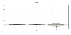
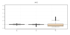
Figure 2: Box-plots displaying ratios of estimates of regression coefficients and area specific sampling variances to their corresponding true values under repeated sampling in our model-based simulation experiment; left and right panels use the proposed algorithm and ML method, respectively; different rows of the panel graph correspond to different simulation scenarios.

We now study the effects of violation of the exchangeability of the regression coefficients and sampling variance components across areas in the nested error regression model of Battese et al., (1988) on the REML estimates of the shrinkage factors $B_{i}$. For different simulation conditions, Figure 3 compares proposed estimates of $B_{i}$, under our nested error regression model with high dimensional parameter (3), with the REML estimates of $B_{i}$ under the nested error regression model of (Battese et al.,, 1988). Under scenario $(0,0)$, i.e., when the nested error model of Battese et al., (1988) is indeed the correct model, the REML estimates of $B_{i}$, obtained under the correct model, perform slightly better than our proposed estimates under the nested error model with high dimensional parameter. When the regression coefficients or/and the sampling variances vary across the areas, the estimates of $B_{i}$ under the nested error model with high dimensional parameter exhibit considerably less bias than the REML under the nested error model at the expense of more variability.

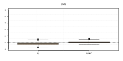
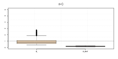
Figure 3: Boxplots displaying ratios of estimates of $B_{i}$ to their corresponding true values under repeated sampling in our model-based simulation experiment; three graphs correspond to the three simulation scenarios; in each graph, estimates of nested regression model with high dimensional parameter and nested error regression model of (Battese et al.,, 1988) are denoted by $B_{i}$ and $B_{i}BHF$, respectively.

Table 1 reports the median values of the ARB, RRMSE and EFF for the various simulation scenarios and estimators. The proposed EBP exhibits the least ARB among all predictors for scenarios $(\beta,0)$ and $(\beta,\sigma_{\varepsilon}^{2})$. As expected, for simulation scenario $(0,0)$, i.e. for the nested error regression model, the EBLUP performs the best in terms of RRMSE. In contrast, when either slopes or both slopes and the sampling variances vary across small areas we note that the proposed EBP performs much better than other predictors in terms of RRMSE. If we compare the EBP with EBP-MLE, the EBP shows the best performance in terms of RRMSE whereas the EBP-MLE exhibits lowest bias values. In the second and third scenarios, the bias and variability of the OBP are similar to those of EBLUP under the nested error regression model. In our simulation experiment, we observe poor performance of the OBP with unit level covariates, as given in Jiang et al., (2011) and Jiang et al., (2015), unless the within area sample sizes are large. However, for the second and third scenarios, the bias and variability of the OBP with area level covariates are similar to those of EBLUP. Thus, in Table 1, we only report results of OBP with area level covariates.

The results presented in Table 1 are supported by the results from two additional simulation experiments. First, we replicated the experiment for $n_{i}=10$ and $m=40$. The results (reported in the Supplementary Material) are similar to those of Table 1, i.e., the proposed EBP exhibits smaller bias and higher efficiency compared to rival small area predictors. As expected, RRMSEs and absolute relative biases for all predictors decrease with the increase of area specific sample sizes.

Moreover, in the second additional experiment, for assessing the performance of the proposed EBP in case of outlying values, we have mixed the scenarios of Chambers et al., (2014) with the ones proposed in this article. The EBP exhibits better performance in terms of both bias and variability compared to the other predictors. The results are reported in Supplementary Material for $n_{i}=5$ and $m=100$ and for $n_{i}=10$ and $m=40$.

Table 1: Model-based simulation results: performance of estimators/predictors of small area means; the number of small areas considered is $100$; population and sample sizes for each area are $100$ and $4$, respectively; median is over 100 small areas; numbers in parenthesis are the values of the efficiency over EBLUP in terms of RMSE.

Predictor Results ($\%$) for the following scenarios $(0,0)$ $(\beta,0)$ $(\beta,\sigma_{\varepsilon}^{2})$ Median absolute relative bias Direct 0.535 0.927 1.083 EBLUP 0.132 9.129 9.155 MQ 0.127 5.070 7.315 EBLUP-RS 0.120 0.672 0.783 EBLUP-H 0.130 8.876 8.903 OBP 0.222 8.691 9.074 EBP 0.136 0.634 0.671 EBP-MLE 0.183 0.232 0.271 Median RRMSE Direct 16.640 (17.887) 44.259 (1.074) 45.770 (1.083) EBLUP 3.922 (1.000) 43.119 (1.000) 44.188 (1.000) MQ 4.105 (1.103) 14.774 (0.132) 20.101 (0.186) EBLUP-RS 3.931 (1.006) 13.991 (0.103) 18.283 (0.144) EBLUP-H 3.924 (1.003) 50.139 (1.359) 53.093 (1.291) OBP 6.969 (3.152) 43.273 (1.001) 44.287 (1.002) EBP 4.002 (1.047) 12.065 (0.087) 15.596 (0.118) EBP-MLE 5.279 (1.798) 14.357 (0.108) 18.685 (0.147)

We now examine the performance of our proposed bootstrap and McJack estimators of RMSE of EBP in comparison with that of the naive RMSE estimator that uses $g_{1i}(\hat{\phi}_{i})$ given by (17). The bootstrap and the McJack procedures have been implemented by generating $100$ bootstrap samples in each Monte Carlo run. The data are generated according to scenarios $(0,0)$, $(\beta,0)$, and $(\beta,\sigma_{\varepsilon}^{2})$. The proposed McJack procedure for the nested error regression model with high dimensional parameter is very computational intensive because for each area $R$ bootstrap iterations are needed. For this reason, to evaluate the performance of the RMSE estimators, we have decided to decrease the number of small areas from $100$ to $40$. The median values of area-specific relative biases (RB) and relative root mean squared errors (RRMSE) of different estimators of RMSE are displayed in Table 2. The table also reports the median values of empirical coverage rates (CR) for nominal $95\%$ confidence intervals of small area means, where confidence intervals are constructed using different RMSE estimators. In the case of naive and and McJack RMSE estimators, these confidence intervals are constructed using the small area estimate plus or minus twice the value of the of the corresponding RMSE estimates. The bootstrap confidence intervals are based on the $2.5$ and the $97.5$ percentiles of the corresponding bootstrap distributions. Compared to the naive RMSE estimator, the bootstrap and McJack RMSE estimators are more stable and less bias and provide confidence intervals with coverage rates. The McJack RMSE estimator provides slightly better performance than the bootstrap estimator, but McJack, as stated above, is time consuming.

Table 2: Model-based simulation results: performance of RMSE estimators for the proposed EBP of a small area mean; the number of small areas considered is $40$; population and sample sizes for each area are $100$ and $10$, respectively; median is over 40 small areas.

RMSE estimator Results ($\%$) for scenarios $(0,0)$ $(\beta,0)$ $(\beta,\sigma^{2})$ Median relative bias Naive -14.9 -23.9 -25.2 Bootstrap -3.6 -8.1 -11.7 McJack -4.9 -4.8 -4.9 Median RRMSE Naive 18.4 30.2 32.5 Bootstrap 14.5 26.4 28.7 McJack 14.1 27.4 26.8 Median coverage rate Naive 91 84 84 Bootstrap 94 93 92 McJack 93 93 94

7.2 Design-based simulation

We use data collected in the 1995-1996 Australian Agricultural Grazing Industry Survey (AAGIS), conducted by the Australian Bureau of Agricultural and Resource Economics. In the original sample there were 759 farms from 12 regions (small areas of interest), which make up the wheat-sheep zone for Australian broad-acre agriculture. We use this sample data to generate a synthetic population of size $N=39,562$ farms by inflating the original AAGIS sample of $n=759$ farms by farm’s sample weight (Salvati et al., 2012a, ). In our simulation, we define the 12 regions as small areas of interest. We know that the proposed nested error regression model with high dimensional parameter and the EBP can work well with a large number of small areas. In this simulation experiment we are also interested in assessing the performance of the EBP when the number of regions is small, but the traditional assumptions of linear mixed model do not hold (e.g., regression coefficients and the sampling variances could vary across the areas). The outcome variable of interest is the total cash costs (TCC) with the number of closing sheep stock as the auxiliary variable.

Using this design-based simulation, we (a) compare the performance of different predictors of mean TCC in each region under repeated sampling from a fixed population with the same characteristics as the AAGIS sample, and (b) evaluate the design-consistency properties of the proposed EBP and MQ. In the design-based simulation experiment we also evaluated the performance and the design-consistency property of an alternative MQ estimator of the mean proposed by Tzavidis et al., (2010). The estimator is based on a smearing argument discussed in Chambers and Dunstan, (1986). Tzavidis et al., (2010) noted that the estimator is subject to severe bias under the linear M-quantile regression model. The MQ estimator based on a smearing argument (hereafter MQCD) may be written as

$$\hat{\theta}_{i}^{MQCD}=\bar{y}_{i}+(\bar{{\mathbf{X}}}_{i}-\bar{{\mathbf{x}}}_{i})^{\prime}\hat{\boldsymbol{\beta}}_{i},$$ (20)

where the vector $\boldsymbol{\beta}_{i}$ is estimated by a method proposed by Chambers and Tzavidis, (2006). It resembles a GREG estimator of the small area mean, which is consistent under the assumption of simple random sampling or some other self-weighting design. Starting from equation (4) the EBP can be written as:

$$\hat{\theta}_{i}^{EBP}=\bar{y}_{i}+(\bar{{\mathbf{X}}}_{i}-\bar{{\mathbf{x}}}_{i})^{\prime}\hat{\boldsymbol{\beta}}_{i}-\hat{B}_{i}(\bar{y}_{i}-\hat{\beta}_{0}-{\bar{{\mathbf{x}}}}_{i}^{\prime}\hat{\boldsymbol{\beta}}_{i}).$$ (21)

We can point out that estimators (20) and (21) are similar. The EBP may be written as MQCD plus a component, $-\hat{B}_{i}(\bar{y}_{i}-\hat{\beta}_{0}-{\bar{{\mathbf{x}}}}_{i}^{\prime}\hat{\boldsymbol{\beta}}_{i})$, representing a part of the estimated specific-area random effect. For this reason we are interested in this design-based simulation experiment to evaluate the performance of MQCD.

For this simulation, we consider $1,000$ independent stratified random samples, each with regional sample sample size of $n_{i}=5$. This results in a total sample size of $60$ locations within the 12 AAGIS regions. The experiment has been replicated with $n_{i}=10,\leavevmode\nobreak\ 15,\leavevmode\nobreak\ 20,\leavevmode\nobreak\ 30,\leavevmode\nobreak\ 40$ and $50$ for evaluating the design consistency.

We compute the relative bias (RB) and the relative root mean squared error (RRMSE) of each estimator/predictor of the mean value of TCC in each region. Figure 4 displays median (over small areas) simulated RB and RRMSE of the estimators/predictors for different area specific sample sizes. The median bias of EBP is lower than those of MQ, EBLUP, EBLUP-H, OBP, EBP-MLE. In terms of median RRMSE criterion, EBP performs the best among all estimators/predictors considered for all sample sizes. EBP outperforms the MQCD in terms of efficiency especially with small sample size. As expected, the difference between RRMSE of EBP and that of MQCD decreases as sample size increases. The design consistency property of an estimator is better demonstrated if we focus on Figure 5, which displays simulated RB and RRMSE by area-specific sample size for the area with smallest population size ($N_{i}=1450$). We note that with the increase of area specific sample size, the simulated RB of EBP (or EBLUP) and MQCD approaches to zero – this is in line with their design consistency property. This is, however, not the case with the MQ – even for large area specific sample size, the simulated RB of MQ is significant. For this specific small area, EBP is a winner with respect to RRMSE criterion.

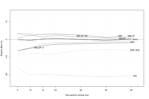
Figure 4: Design-based simulation results: median of relative bias (top panel) and relative root mean squared error (bottom panel) of the small area predictors by area-specific sample size.

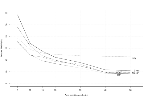
Figure 5: Design-based simulation results for area with smallest $N_{i}$: relative bias (top panel) and relative root mean squared error (bottom panel) of the small area predictors by area-specific sample size.

8 An application of the high dimensional parameter linear mixed model: EBP estimates of the ecological condition of lakes in the northeastern USA

We use as illustrative example the data collected from EMAP and presented in Section 2. Predicted values of average ANC for each HUC are calculated using the empirical version of (4) under the nested error regression model with high dimensional parameter (3) with covariates equal to the elevation of each lake and location defined by the geographical coordinates of the centroid of each lake (in the UTM coordinate system).

Figure 6 shows normal probability plots of level 1 transformed residuals ($u_{ij}$, Battese et al.,, 1988) and level 2 standardized random effects (Lange and Ryan,, 1989) obtained by fitting a two-level (level 1 is the lake and level 2 is the HUC) linear mixed model to the sample data. The normal probability plots indicate that the Gaussian assumptions of the linear mixed model are not met. This is confirmed by a Shapiro-Wilk normality test, which rejects the null hypothesis that the residuals follow a normal distribution ($p$-values: level 1 = 2.2e-16, level 2 = 0.0006247).

Figure 6: Normal probability plots of level 1 (left) and level 2 residuals (right) derived by fitting a two level linear mixed model to sample data.

Following Zewotir and Galpin, (2007) we study the detection of outliers and high leverage points in the sample data. The authors propose to use the diagonal elements $s_{ii}$ of the matrix ${\mathbf{S}}=\sigma_{\varepsilon}^{2}{\mathbf{P}}$, with ${\mathbf{P}}={\mathbf{V}}^{-1}-{\mathbf{V}}^{-1}{\mathbf{X}}({\mathbf{X}}^{\prime}{\mathbf{V}}^{-1}{\mathbf{X}})^{-1}{\mathbf{X}}^{\prime}{\mathbf{V}}^{-1}$ (where ${\mathbf{X}}$ is the design matrix and ${\mathbf{V}}$ is the covariance matrix of the linear mixed model), to detect high leverage points. To detect both outliers and high leverage points, they propose to examine a plot of $s_{ii}$ versus $\hat{\varepsilon}_{i}^{2}/\hat{\boldsymbol{\varepsilon}}^{\prime}\hat{\boldsymbol{\varepsilon}}$, where $\hat{\varepsilon}_{i}$ is the EBLUP residual. Points are expected to concentrate around the upper-left corner of the plot. Points separated from the main cloud of points that fall in the lower-left corner (small $s_{ii}$) are regarded as high leverage points, and points that appear separated on the right side (large relative squared $\hat{\varepsilon}_{i}^{2}/\hat{\boldsymbol{\varepsilon}}^{\prime}\hat{\boldsymbol{\varepsilon}}$) are regarded as outliers. Using in Figure 7 the rough cutoff values proposed by Zewotir and Galpin, (2007) we note the presence of both outliers and high leverage points in the EMAP data.

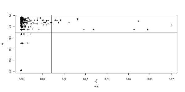
Figure 7: Plot to detect both outliers and high leverage points: $s_{ii}$ versus $\hat{\varepsilon}_{i}^{2}/\hat{\boldsymbol{\varepsilon}}^{\prime}\hat{\boldsymbol{\varepsilon}}$.

These diagnostics suggest the use of a robust model that relaxes the assumptions of normality of the linear mixed model. The model (3) is fitted on the EMAP data by setting the value of the tuning constant in the Huber influence function to $c=1.345$. We have studied the stability of our algorithm, i.e., we have ensured that the convergence of the algorithm does not depend on the starting values. For the data we used in this paper, when initialising the algorithm from different starting values, it always converged to the same point. However, in some applications, convergence may not be stable due to sparsity of the data. Hence, users of the method should always test the convergence of the algorithm with their data sets to ensure that there are no convergence problems.

From the estimates there is evidence of spatial variability of the regression coefficients and variance components. Figure 8 shows contour maps of the estimated HUC-specific area elevation slope coefficient (left) and error variance model (right) from the fitted varying model. Examining the contours of the slope coefficients in Figure 8 we see that the effect of elevation on ANC varies spatially, with these slope coefficients ranging from $-2.5$ to $-0.45$. The error variance component also shows spatial variation. In particular, the contour map of this component shows them ranging from a value close to $0$ (East) to $50,000$ (West).

Figure 8: Maps showing the spatial variation in the HUC-specific area elevation slope coefficient (left) and sampling variance (right) estimates that are generated when the proposed nested error regression model with high dimensional parameter is fitted to the EMAP data.

These results are confirmed by the Hausman test (Hausman,, 1978; Battese et al.,, 1988), where the null hypothesis that slope parameters are the same within and among areas is rejected ($p$-value= 0.0021) and by the Raudenbush and Bryk’s test (Raudenbush and Bryk,, 2002), where the null hypothesis of equality of the $\sigma_{\varepsilon}^{2}$ between areas is rejected ($p$-value= 8e-04).

To assess how EBP estimates are ‘close’ to the direct estimates we compute a goodness-of-fit diagnostic (Brown et al.,, 2001). This allows for evaluating if the model-based estimates are more precise than direct estimates. The goodness-of-fit diagnostic is computed as the value of the following Wald statistic:

$$W=\sum_{i}\frac{(\bar{y}_{i}-\hat{\theta}_{i}^{EBP})^{2}}{\widehat{var}(\bar{y}_{i})+\widehat{MSE}(\hat{\theta}_{i}^{EBP})},$$

where $\widehat{var}(\bar{y}_{i})$ is the estimated variance of the direct estimator and $\widehat{MSE}(\hat{\theta}_{i}^{EBP})$ is the estimated MSE of the EBP computed via bootstrap procedure. The realized value of $W$ can then be compared against the $0.95$-quantile of a $\chi^{2}$-distribution with 86 degrees of freedom, i.e. $108.6479$. The values of the goodness-of-fit diagnostic is $19.21$ for EBP, i.e. the estimates are not statistically different from the direct estimates. The EBP estimates appear to be generally consistent with the direct estimates, with the correlation between the two sets of estimates being $0.98$. To assess if EBP estimates are more precise than direct estimates, i.e. the potential gains in precision from using EBP instead of the direct estimates, we examine the distribution of the ratios of the estimated CVs of the direct and the EBP estimates for the EMAP data. A value greater than 1 for this ratio indicates that the estimated CV of the EBP estimate is smaller than that of the direct estimate. The average ratio across areas is $1.83$. It means a potential gain in precision from using EBP of about $83\%$.

Estimated values of average ANC for each HUC using EBP under the nested regression model with high dimensional parameter indicate that there are lower levels of average ANC (higher risk of water acidification) in the north-eastern part of the study region and they are consistent with the spatial distribution of ANC average values produced by previous non-parametric analyses of the EMAP data Opsomer et al., (2008) and Salvati et al., 2012b .

In Figure 9 we display maps of estimates of average ANC for each HUC using EBP under the nested error model with high dimensional parameter. Estimates indicate that there are lower levels of average ANC (higher risk of water acidification) in the north-eastern part of the study region and they are consistent with the spatial distribution of ANC average values produced by previous non-parametric analyses of the EMAP data (Opsomer et al.,, 2008; Salvati et al., 2012b, ).

Figure 9: Maps of estimated average ANC for HUCs using EBP under the nested error regression model with high dimensional parameter.

9 Conclusions

In this paper, we have demonstrated, through simulations and data analysis, unsuitability of the well-known nested error regression model for small area estimation when combining a large number of small areas. As argued in the paper, this could be due to the fact that the exchangeability assumption concerning the regression coefficients and fixed sampling variances does not hold for large number of small areas to be combined. One potential solution to this problem is develop methodology for a joint random regression coefficients and random sampling variances model. Such joint modeling strategy has not been tried in the small area literature and could be an excellent future research problem. Alternatively, one could consider allowing fixed area specific regression coefficients and sampling variances to circumvent problems associated with exchangeability of the regression coefficients and sampling variances across small areas. However, this modeling strategy is likely to lead to an inefficient estimation of the area specific regression coefficients and sampling variances if traditional estimation methods are used because of small area specific samples. In this paper, we develop a robust area specific estimating equations approach where different estimating equations are used for different small areas. Random effect is assumed on a single area specific tuning parameter of the estimation equation (e.g., $\tau_{i}$, area specific M-quantile coefficient) to reduce dimensionality, which in turn, improves on estimation efficiency.

Performances of the estimators of area specific regression coefficients and sampling variances $\phi_{i}$ and the associated EBP depend very much on the area specific tuning parameters $\tau_{i}$ of the estimating equations. The case when $\tau_{i}$’s are known (e.g., from the census data) does not create any problem. Like in many other papers in small area estimation, our emphasize here is bounded $n_{i}$ and our evaluation for unknown $\tau_{i}$ case is exclusively by extensive simulation studies, which actually allow us to consider a variety of simulation conditions. In most SAE asymptotics, $m$ tends to infinity but $n_{i}$’s are bounded. In such a setting, the estimators of $\tau_{i}$ considered in this paper are not consistent. As pointed out by Jiang and Lahiri (2006), the alternative asymptotic setting in which both number of areas $m$ and area specific sample sizes $n_{i}$ tend to (possibly at differential rates) is indeed an important problem. This alternative asymptotic framework has received relatively less attention in SAE research. Lye and Welsh (2021) recently put forward an asymptotic approach where both $m$ and $n_{i}$ are allowed to tend to infinity. It would be interesting to study the asymptotic properties of our estimators of our model parameters and predictors under this alternative asymptotic setting. This is a topic for a future research.

In this paper, we also question the utility of the well-known second-order unbiasedness criterion of the mean squared error estimators. Besides the difficulty in establishing a rigorous theory (see Jiang et al.,, 2018) and increasing the computational burden, this property does not necessarily ensure similar second-order unbiasedness properties of other commonly used uncertainty measures such as coefficient of variation, relative root mean squared error, and others. In this paper, we downplay the second-order unbiasedness criterion and introduces a general parametric bootstrap method and a jackknife procedure for estimating commonly used uncertainly measures such as relative root mean square error and coefficient of variance. Proposed methods perform well in our Monte Carlo simulations and real life data analysis. In developing the methodology we ignored certain complex situations such as correlated data within the same PSU. Also, the method is developed for continuous data. These present additional avenues for further research. Finally, as alternative to the proposed nested error regression model with high dimensional parameter, an extension of linear models with both random coefficients and random dispersion values in Bayesian approach following Hoff, (2009, Chapter 8) may be doable and it could be an objective of a future research.

Acknowledgments: The word of P. Lahiri was partially supported by the U.S. National Science Foundation grant SES- 1758808. The work of N. Salvati has been developed under the support of the Progetto di Ricerca di Ateneo From survey-based to register-based statistics: a paradigm 345 shift using latent variable models’ (grant PRA2018-9). The work of Salvati was carried out with the support of the project InGRID-2 Integrating Research Infrastructure for European expertise on Inclusive Growth from data to policy (Grant Agreement N. 730998, EU)

Appendix: Regularity conditions for consistency of the estimators of $\boldsymbol{\phi}_{i}$

• The influence function $\psi_{i}$ is a bounded continuous function with a derivative which, except for a finite number of points, is defined everywhere and it is also bounded.

• $|{\mathbf{X}}_{l(p+1)}|$, $1\leqslant l\leqslant m$, is bounded as $m\rightarrow\infty$.

• The true parameter vector $\boldsymbol{\phi}_{i}\in\boldsymbol{\Phi}_{i}^{0}$, the interior of the parameter space for $\boldsymbol{\phi}_{i}$.

• For any compact set ${\mathbf{B}}\in\boldsymbol{\Phi}_{i}^{0}$, the $sup_{\boldsymbol{\phi}_{i}\in{\mathbf{B}}}||\cdot||$ of up to fourth derivatives of ${\mathbf{V}}_{i}$, $1\leqslant i\leqslant m$, are bounded, and $sup_{\boldsymbol{\phi}_{i}\in{\mathbf{B}}}||{\mathbf{V}}_{i}||$, $1\leqslant i\leqslant m$, are bounded.

• $\lambda_{min}\{{\mathbf{X}}_{l(p+1)}^{\prime}{\mathbf{U}}_{l;i}^{-1/2}{\mathbf{D}}_{l;i}{\mathbf{U}}_{l;i}^{1/2}{\mathbf{V}}_{l;i}^{-1}{\mathbf{X}}_{l(p+1)}\}$, $\lambda_{min}\left\{tr\left[{\mathbf{V}}_{l;i}^{-1}{\mathbf{Z}}_{l}{\mathbf{Z}}_{l}^{\prime}{\mathbf{V}}_{l;i}^{-1}{\mathbf{Z}}_{l}{\mathbf{Z}}_{l}^{\prime}\right]\right\}$ and $\lambda_{min}\left\{tr\left[{\mathbf{V}}_{l;i}^{-1}\frac{\partial{\mathbf{V}}_{l;i}}{\partial\sigma_{\epsilon i}^{2}}|_{\sigma_{\gamma}^{2}=\sigma_{\gamma}^{2}}{\mathbf{V}}_{l;i}^{-1}\frac{\partial{\mathbf{V}}_{l;i}}{\partial\sigma_{\epsilon i}^{2}}|_{\sigma_{\gamma}^{2}=\sigma_{\gamma}^{2}}\right]\right\}$ are bounded away from zero, where $\lambda_{min}$ represents the smallest eigenvalue; here ${\mathbf{D}}_{l;i}$ is a diagonal matrix with its $j$th diagonal element is the derivative of $\psi_{i}$ respect the $j$th residual;

• There are constants $\zeta>0$ and $L<\infty$ such that, if ${\mathbf{r}}_{l;i}$, $1\leqslant l\leqslant m$, then $E|\psi_{i}({\mathbf{r}}_{l;i})|^{4+\zeta}$, $E||\partial\psi_{i}({\mathbf{r}}_{l;i})||$ are all bounded by $L$.

• $E|{\mathbf{y}}_{l}|^{8+\varphi}$, $1\leqslant l\leqslant m$, are bounded for some $\varphi>0$.

• $|S|=O(m^{\kappa})$ for some $0\leqslant\kappa\leqslant 3/(6+\varphi)$.

References

- Arora et al., (1997) Arora, V., Lahiri, P., and Mukherjee, K. (1997). Empirical bayes estimation of finite population means from complex survey. Journal of the American Statistical Association, 92:1555–1562.
- Bates et al., (2015) Bates, D., Mächler, M., Bolker, B., and Walker, S. (2015). Fitting linear mixed-effects models using lme4. Journal of Statistical Software, 67(1):1–48.
- Battese et al., (1988) Battese, G. E., Harter, R. M., and Fuller, W. A. (1988). An error component model for prediction of county crop areas using survey and satellite data. Journal of the American Statistical Association, 83 (401):28–36.
- Bianchi and Salvati, (2015) Bianchi, A. and Salvati, N. (2015). Asymptotic properties and variance estimators of the m-quantile regression coefficients estimators. Communications in Statistics - Theory and Methods, 44:2416–2429.
- Breckling and Chambers, (1988) Breckling, J. and Chambers, R. (1988). M-quantiles. Biometrika, 75 (4):761–771.
- Brown et al., (2001) Brown, G., Chambers, R., Heady, P., and Heasman, D. (2001). Cevaluation of small area estimation methods—an application to unemployment estimates from the uk lfs. In Symp, P. S. C., editor, Achieving Data Quality in a Statistical Agency: a Methodological Perspective, Hull: Statistics Canada.
- Chambers et al., (2014) Chambers, R., Chandra, H., Salvati, N., and Tzavidis, N. (2014). Outlier robust small area estimation. Journal of the Royal Statistical Society: Series B, 76 (1):47–69.
- Chambers and Dunstan, (1986) Chambers, R. and Dunstan, R. (1986). Estimating distribution functions from survey data. Biometrika, 73:597–604.
- Chambers and Tzavidis, (2006) Chambers, R. and Tzavidis, N. (2006). M-quantile models for small area estimation. Biometrika, 93 (2):255–268.
- Chandra et al., (2012) Chandra, H., Salvati, N., Chambers, R., and Tzavidis, N. (2012). Small area estimation under spatial nonstationarity. Computational Statistics and Data Analysis, 56:2875–2888.
- Das et al., (2004) Das, K., Jiang, J., and Rao, J. (2004). Mean squared error of empirical predictor. The Annals of Statistics, 32 (2):818–840.
- Datta and Lahiri, (2000) Datta, G. S. and Lahiri, P. (2000). A unified measure of uncertainty of estimated best linear unbiased predictors in small area estimation problems. Statistica Sinica, 10:613–627.
- Fabrizi et al., (2014) Fabrizi, E., Salvati, N., Pratesi, M., and Tzavidis, N. (2014). Outlier robust model-assisted small area estimation. Biometrical Journal, 56:157–175.
- Ghosh, (2020) Ghosh, M. (2020). Small area estimation: Its evolution in five decades. Statistics in Transition New Series, Special Issue on Statistical Data Integration, pages 1–67.
- Ghosh and Lahiri, (1987) Ghosh, M. and Lahiri, P. (1987). Robust empirical bayes estimation of means from stratified samples. Journal of the American Statistical Association, 82:1153–1162.
- Ghosh and Meeden, (1997) Ghosh, M. and Meeden, G. (1997). Bayesian Methods for Finite Population Sampling. Chapman & Hall, London.
- Hall and Maiti, (2006) Hall, P. and Maiti, T. (2006). On parametric bootstrap methods for small area prediction. Journal of the Royal Statistical Society: Series B, 68 (2):221–238.
- Hausman, (1978) Hausman, J. (1978). Specification tests in econometrics. Econometrica, 46(6):1251–1271.
- Higgins, (1993) Higgins, R. M. (1993). A robust approach to the analysis of repeated measures. Biometrics, 49:715–720.
- Hobza and Morales, (2013) Hobza, T. and Morales, D. (2013). Small area estimation under random regression coefficient models. Journal of Statistical Computation and Simulation, 83 (11):2160–2177.
- Hoff, (2009) Hoff, P. (2009). A first course in Bayesian statistical methods, volume 580. Springer.
- Huber, (1981) Huber, P. (1981). Robust Statistics. Wiley, New York.
- Jiang, (2017) Jiang, J. (2017). Asymptotic Analysis of Mixed Effects Models: Theory, Application, and Open Problems. Chapman & Hall/CRC, New York.
- Jiang and Lahiri, (2006) Jiang, J. and Lahiri, P. (2006). Mixed model prediction and small area estimation. Test, 15 (1):1–96.
- Jiang et al., (2018) Jiang, J., Lahiri, P., and Nguyen, T. (2018). A unified monte-carlo jackknife for small area estimation after model selection. Annals of Mathematical Sciences and Applications, 3 (2):405–438.
- Jiang et al., (2002) Jiang, J., Lahiri, P., and Wan, S.-M. (2002). A unified jackknife theory for empirical best prediction with M-estimation. The Annals of Statistics, 30:1782–1810.
- Jiang and Nguyen, (2012) Jiang, J. and Nguyen, T. (2012). Small area estimation via heteroscedastic nested-error regression. Canadian Journal of Statistics, 40:588–603.
- Jiang et al., (2011) Jiang, J., Nguyen, T., and Rao, J. (2011). Best predictive small area estimation. Journal of the American Statistical Association, 106:732–745.
- Jiang et al., (2015) Jiang, J., Nguyen, T., and Rao, J. (2015). Observed best prediction via nested-error regression with potentially misspecified mean and variance. Survey Methodology, 41:37–55.
- Koenker, (2005) Koenker, R. (2005). Quantile Regression. Cambridge University Press, New York.
- Kubokawa et al., (2016) Kubokawa, T., Sugasawa, S., Ghosh, M., and Chaudhuri, S. (2016). Prediction in heteroscedastic nested error regression models with random dispersions. Statistica Sinica, 26:465–492.
- Lange and Ryan, (1989) Lange, N. and Ryan, L. (1989). Assessing normality in random effects models. The Annals of Statistics, 17 (2):624–642.
- Larsen et al., (2001) Larsen, D., Kincaid, T., Jacobs, S., and Urquhart, N. (2001). Designs for evaluating local and regional scale trends. Bioscience, 51:1049–1058.
- Liu et al., (2014) Liu, B., Lahiri, P., and Kalton, G. (2014). Hierarchical bayes modeling of survey-weighted small area proportions. Survey Methodology, 40 (1):1–13.
- Naves et al., (2020) Naves, A., Silva, D., and Moura, F. (2020). Small area estimation: Its evolution in five decades. Statistics in Transition New Series, Special Issue on Statistical Data Integration.
- Neyman and Scott, (1948) Neyman, J. and Scott, E. (1948). Consistent estimates based on partially consistent observations. JEconometrica, 16(1):1–32.
- Opsomer et al., (2008) Opsomer, J., Claeskens, G., Ranalli, M., Kauermann, G., and Breidt, F. (2008). Nonparametric small area estimation using penalized spline regression. Journal of the Royal Statistical Society: Series B, 70:265–283.
- Otto and Bell, (1995) Otto, M. C. and Bell, W. R. (1995). Sampling error modelling of poverty and income statistics for states. In American Statistical Association, Proceedings of the Section on Government Statistics, pages 160–165.
- Pfeffermann, (2013) Pfeffermann, D. (2013). New important developments in small area estimation. Statistical Science, 28 (1):40–68.
- Prasad and Rao, (1990) Prasad, N. G. N. and Rao, J. N. K. (1990). The estimation of the mean squared error of small area estimators. Journal of the American Statistical Association, 85 (409):163–171.
- Rao and Molina, (2015) Rao, J. N. K. and Molina, I. (2015). Small Area Estimation. Wiley, New York, 2nd edition edition.
- Raudenbush and Bryk, (2002) Raudenbush, S. and Bryk, A. (2002). Hierarchical Linear Models: Applications and Data Analysis Methods. Sage, Thousand Oaks, 2nd edition.
- Richardson and Welsh, (1995) Richardson, A. M. and Welsh, A. H. (1995). Robust restricted maximum likelihood in mixed linear models. Biometrics, 51 (4):1429–1439.
- (44) Salvati, N., Chandra, H., and Chambers, R. (2012a). Model-based direct estimation of small-area distributions. Australian and New Zealand Journal of Statistics, 54 (1):103–123.
- Salvati et al., (2021) Salvati, N., Fabrizi, E., Ranalli, M., and Chambers, R. (2021). Small area estimation with linked data. Journal of the Royal Statistical Society: Series B, 83(1):78–107.
- (46) Salvati, N., Tzavidis, N., pratesi, M., and Chambers, R. (2012b). Small area estimation via m-quantile geographically weighted regression. TEST, 21(1):1–28.
- Sugasawa and Kubokawa, (2017) Sugasawa, S. and Kubokawa, T. (2017). Heteroscedastic nested error regression models with variance functions. Statistica Sinica, 27(3):1101–1123.
- Sugasawa et al., (2017) Sugasawa, S., Tamae, H., and Kubokawa, T. (2017). Bayesian estimators for small area models shrinking both means and variances. Scandinavian Journal of Statistics, 44(1):150–167.
- Tzavidis et al., (2010) Tzavidis, N., Marchetti, S., and Chambers, R. (2010). Robust estimation of small area means and quantiles. Australian and New Zealand Journal of Statistics, 52 (2):167–186.
- Venables and Ripley, (2002) Venables, W. and Ripley, B. (2002). Modern applied statistics with S. Springer, New York.
- Zewotir and Galpin, (2007) Zewotir, T. and Galpin, J. (2007). A unified approach on residuals, leverages and outliers in the linear mixed model. TEST, 16:58–75.