Active polar flock with birth and death

Abstract

We study a collection of self-propelled polar particles on a two-dimensional substrate with birth and death. We introduce a minimal lattice model for the system using active Ising spins, where each particle can have two possible orientations. The activity is modeled as a biased movement of the particle along its direction of orientation. The particles also align with their nearest neighbors using Metropolis Monte-Carlo algorithm. System shows a disorder-to-order transition by tuning the temperature of the system. Additionally, the birth and death of the particles is introduced through a birth and death rate $\gamma$. The system is studied near the disorder-to-order transition. The nature of disorder-to-order transition shows a crossover from first order, discontinuous to continuous type as we tune $\gamma$ from zero to finite values. We also write the effective free energy of the local order parameter using renormalised mean field theory and it confirms the dependence of the nature of phase transition on the birth and death rate parameter.

I Introduction

The active matter systems can be recognised as a collection of particles in which the individual components possess non-zero motility by converting the energy from its surroundings and also from the medium Toner et al. (2005); Toner and Tu (1995, 1998a, 1998b); Bechinger et al. (2016); Vicsek and Zafeiris (2012). The active particles spontaneously self organize when present in large numbers, and results in coordinated and collective behavior (CB) on various length scales Gompper et al. (2020); Toner and Tu (1998b); Bechinger et al. (2016); Saintillan (2010); Shen and Wolynes (2004); Dombrowski et al. (2004); Kemkemer et al. (2000); Surrey et al. (2001); Bendix et al. (2008). The phenomenon of collective behavior is being studied with great interest in systems exhibiting nonequilibrium phase transition under driven noise and particle density Toner and Tu (1995); Chaté et al. (2008); Buttinoni et al. (2013); Bhattacherjee et al. (2015); Pattanayak and Mishra (2018); Singh et al. (2021). In different studies of active matter systems it has been shown that the system changes its properties such as pattern of the structure, nature of the phase transition by tuning the interaction among the particles Toner and Tu (1998b); Bhattacherjee et al. (2015); Pattanayak and Mishra (2018); Singh et al. (2021); Durve and Sayeed (2016); Giomi et al. (2010); Ramaswamy et al. (2003). Among them the nature of phase transition is one of the most studied phenomenon in this field of research Chaté et al. (2008); Bhattacherjee et al. (2015); Pattanayak and Mishra (2018); Singh et al. (2021); Durve and Sayeed (2016); Solon and Tailleur (2013, 2015). The phase transition in the collection of self-propelled particles also called as “flocking transition” is important, because it can be described as a nonequilibrium analog of disorder-to-order phase transition in equilibrium systems Vicsek et al. (1995); Solon and Tailleur (2015, 2013).
In recent study of Solon et. al. Solon and Tailleur (2013), it has been found that the nature of phase transition in self-propelling agents is analogous to the liquid-gas transition on the variation of temperature and density in the system Solon and Tailleur (2013, 2015). To understand the phase transition Solon et. al. introduced a microscopic lattice model with discrete symmetry, which is known as active Ising model $(AIM)$ Solon and Tailleur (2013). The $AIM$ is much simplified model for the collective motion and gives the basic features of the flocking models Solon and Tailleur (2015): viz, band formation, large density fluctuations, discontinuous disorder-to-order phase transition etc. The study of $AIM$ by Solon and Tailleur (2013) is for the system where total number of agents is fixed. The effect of birth and death of agents on the system is not yet explored.
In this current study we ask the question: whether the introduction of birth and death of the agents can affect the nature of phase transition? To serve this purpose, we introduced a minimal lattice based-model of active Ising spins $(AIM)$ with an additional birth and death rate $\gamma$.
The system is studied for various $\gamma$ and it is found that for the $\gamma=0$, the system shows a first order, disorder-to-order phase transition with the appearance of bands in the local density and magnetisation. On introducing the $\gamma$, the bands start to dilute and finally disappear for large $\gamma$ and transition becomes continuous in nature. We also studied the system using coarse-grained hydrodynamic equations of motion. Using renormalised mean field theory we write an effective free energy for local order parameter and find an additional cubic order nonlinearity present for zero birth and death and the nonlinearity weakens on increasing birth and death rate.

The rest of the paper is organized as follows. In Sec. II, we discuss the model and simulation details. In Sec. III, the results from the numerical simulations are discussed where we mainly conclude how the nature of phase transition is changing by tuning the parameter $\gamma$. In addition to numerical approach, we also study the system analytically in Sec. 7 with the help of coarse-grained hydrodynamic equations for density and polarisation using renormalised mean field theory. Finally in Sec. V, we conclude the paper with a summary and discussion of the results.

Figure 1: (color online) (a) Sketch of a part of system carrying spins $S=+1$(red (triangle right)) and $S=-1$(dark green (triangle left)) along with vacant sites S=0(black circle) on a two-dimensional lattice.(b) represents the flipping rate at fixed temperature.(c) represents the probability of movement of the spins to the neighboring sites. (d) birth and death rate $\gamma$ is added in the model in which the particles disappearing from random sites is shown by magenta square and appearing at the sites which were vacant represented by orange triangle right for $S=+1$ and green triangle left for $S=-1$.

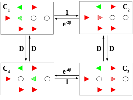
Figure 2: (color online) A loop of four configurations that breaks Kolmogorov’s criterion Kolmogorov (1936) of detailed balance for $dIm$, flipping and movement is shown for the spin represented by partially filled (red (triangle right)) and (dark green (triangle left)). The clockwise loop $(C_{1}$ $\rightarrow$ $C_{2}$ $\rightarrow$ $C_{3}$ $\rightarrow$ $C_{4}$ $\rightarrow$ $C_{1})$ gives the total probability $D^{2}e^{-4\beta}$ while the anticlockwise loop $(C_{1}$ $\rightarrow$ $C_{4}$ $\rightarrow$ $C_{3}$ $\rightarrow$ $C_{2}$ $\rightarrow$ $C_{1})$ gives the total probability $D^{2}e^{-2\beta}$, thus showing that the system does not satisfy detailed balance. The numbers associated to the arrows are the transition rates and other symbols have the same meaning as in Fig.1.

II Model and numerical details

We consider a system of active Ising spins $(AIM)$ on a two-dimensional rectangular lattice of size $L_{x}$ $\times$ $L_{y}$ with periodic boundary condition in both directions. A fraction of sites on the lattice is vacant. Each spin can take two possible values $S_{i}=\pm 1$. Some of the sites are vacant hence we define an occupancy variable $n_{i}=0$ or $1$ for the unoccupied and occupied sites respectively. Each site can have maximum one particle on it. Hence, unlike the previous $AIM$ introduced by Solon et. al. our spins have mutual exclusion among them mut . Each spin can interact with its nearest neighbor spins using the Ising Hamiltonian Ising (1925)

$$H=-\sum_{i=1}^{N}n_{i}n_{j}S_{i}S_{j},$$ (1)

hence the interaction term is non-zero only if the site and the interacting sites both are occupied. The above Hamiltonian Eq. 1 is simulated for a fixed vacancy density $V=20\%$ (particle density $\rho=0.8$) by tuning the temperature. The temperature is introduced through the Metropolis Monte-Carlo algorithm Landau and Binder (2005); Pathria and Beale (2011) for the alignment interaction among the spins. The ratio of the interaction strength and the Boltzmann constant is chosen as $1$. The dynamics of the spins on the lattice can be modeled in the following manner: (i) the spins are fixed to their lattice sites $(fIm)$ and interacts through the Hamiltonian in Eq. 1. (ii) We allowed the spin to diffuse to any of its nearest vacant site with equal probability. The model is named as diffusive Ising model $(dIm)$. In Fig. 2 we show the Kolmogorov diagram Kolmogorov (1936) to check the detail balance condition on $dIm$. In Fig. 2, a loop of four configurations is shown, that breaks Kolmogorov’s criterion, e.g. clockwise loop gives the total probability $D^{2}e^{-4\beta}$ while anticlockwise loop gives $D^{2}e^{-2\beta}$, thus showing that the system does not satisfy detailed balance. The numbers associated to the arrows are the transition rates. Hence $fIm$ satisfies the detail balance condition but the $dIm$ deviates from it.
(iii) Further we made the spins active by introducing a biased movement corresponding to their direction as introduced in Solon and Tailleur (2015, 2013). The update rules showing the motion of the spins is shown in Fig. 1(b). Activity is introduced through a parameter $\epsilon\in(0,1)$. In the presence of activity $\epsilon$, the update rule for the movement of the spins at a particular site is given as follows. Each particle hops to its two neighboring sites left and right at rate $D(1+S\varepsilon)$ provided the target site is vacant. It hops to other two sites (up and down) with equal probablity $D$. If the $\varepsilon=0$, then the hoping rates are same in all the directions and that rate comes out to be $D=1/4$ and the model reduces to $dIm$. For nonzero $\epsilon$, the particle moves in the direction of its orientation at rate $D(1+\varepsilon)$ and in the opposite direction to its orientation at rate $D(1-\varepsilon)$. Whereas the particle hops with rate $D$ to other two possible directions. For our present study we fix $\varepsilon=1.0$. We call the model as active model $(Am)$.
(iv) Next we introduce the birth and death of particles in the model $(Am)$. The birth and death rate $\gamma$ is introduced as a fraction of sites on the lattice with density $\gamma$, such that from the randomly chosen $\gamma/2$ fraction of sites we remove the particles (if occupied) and similarly by another randomly chosen $\gamma/2$, we introduced the new particles with spin favoured with the majority spins in their nearest neighbor. The $\gamma$ is tuned from $0$ to $0.1$. For $\gamma=0$ model reduces to $Am$ and for $\gamma\neq 0$ we call it birth and death active model $(bdAm)$. One simulation step is counted after successful update of the above steps for all the particles once. Total simulation steps (time) used is $T=1.7\times 10^{5}$. The steady state in the system is achieved after simulation time $7\times 10^{4}$. We use $40$ independent realizations for averaging the data for the system size $L_{x}=400$ and $L_{y}=50$.

Figure 3: The plot of order parameter $M$ vs. temperature $T$ for various values of $\gamma$ i.e. The black (circle), red (square), green (diamond), blue (triangle right) and maroon (triangle left) for $\gamma=0$, $\gamma=0.01$, $\gamma=0.1$, $\gamma=0.5$ and $\gamma=1$ respectively. The lines are guide to the eyes.

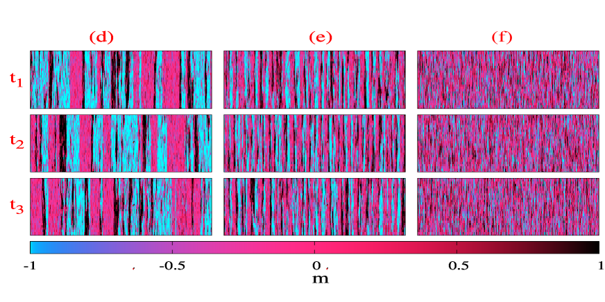
Figure 4: Time snapshots of local density $\rho_{loc}$ (a-c) and local magnetisation $m$ (d-f). From left to right (a-c) or (d-f) is for $\gamma=0.0$, $0.01$ and $0.1$ and ($t_{1}$-$t_{3}$) is for $1.4\times 10^{5}$, $1.5\times 10^{5}$, $1.6\times 10^{5}$ respectively. Color bars represent the value of local density $\rho_{loc}$ and magnetisation $m$.

III Results

We first studied the model $(bdAm)$ with no birth and death rate $\gamma=0$. The system is studied by varying temperature. A disorder-to-order phase transition is found on decreasing temperature. We studied the system for activity $\epsilon=1$ and for different $\gamma$. We first calculated the global magnetisation in the system defined as:-

$$M(t)=\frac{1}{N}\mid\sum_{i}S_{i}(t)\mid$$ (2)

where $N$ is total number of particles. We define the mean magnetisation $M=<M(t)>$, where $<..>$ means the average over time in the steady state and over different realisations. We find that for the high temperature for all $\gamma$ system is disordered and $M\simeq 0$, and ordered with $M\simeq 1$ for low temperature. The variation of $M$ as a function temperature is shown in Fig. 3 for different $\gamma$. We find a very strong dependence of the shape of the disorder-to-order curve on $\gamma$. The shape of the transition curve changes from first order (discontinuous type) to continuous type as we tuned the $\gamma$ from $0$ to $0.1$. Hence, the nature of phase transition changes from first order type to continuous type for large birth and death rate $\gamma$.
To further confirm the nature of transition, we looked the system near to the disorder-to-order transition. We first plot the real space snapshot of local density $\rho_{loc}$ in Fig. 4(a-c). The $\rho_{loc}$ is calculated by counting the density of spins in box of size $2\times 2$. The panels from top to bottom ($t_{1}$ - $t_{3}$) for three different simulation times $t=1.4\times 10^{5}$, $1.5\times 10^{5}$ and $1.6\times 10^{5}$ respectively. The panel (a)-(c) is for $\gamma=0$, $0.01$ and $0.1$ respectively. For $\gamma=0$, we see the formation of bands of high density spins. With time the bands move across the system. The bands get diluted on increasing $\gamma$ and disappear for large $\gamma=0.1$. The color bar shows the value of local density $\rho_{loc}$. Similarly we also plot the local magnetisation $m$, obtained by calculating the mean spin in the box of size $2\times 2$ in Fig. 4(d-f) for the same set of parameters as for (a-c). The panel (d-f) is for $\gamma=0$, $0.01$ and $0.1$ respectively. We again find for zero $\gamma$, bands of high ordered region moves in the background of disordered region. The bands get diluted on increasing $\gamma$ and finally disappear for large $\gamma=0.1$. The color bar shows the value of local $m$ and positive and negative $m$ represents the mean local spin $+1$ and $-1$ respectively. Very clearly the band splits into thinner and weaker bands on the introduction of $\gamma$. The formation of bands we find here for $\gamma=0$ or $Am$ is a common characteristics of polar flock Chaté et al. (2008); Solon and Tailleur (2015, 2013); Mishra et al. (2010). For large $\gamma\simeq 0.1$ slowly the density pattern disappears and its all become close to mean density $\rho_{loc}=0.8$.

To further characterise the density inhomogeneity for different $\gamma$ we plot the distribution of density for different temperatures close to disorder-to-order transition. Using the the local density $\rho_{loc}$ plots shown in Fig. 4(a-c), we calculated the local density along the long axis of the system by averaging over the shorter axis $L_{y}$. In this manner we find the density variation in one direction $\rho_{x}$. We further plot the probability distribution function (PDF) of density $P(\rho_{x})$ for various $\gamma$ in Fig. 5. For zero $\gamma$, distribution clearly shows the bimodal nature, with one peak close to $1$ (maximum density) and another peak at lower density $\rho_{x}=0.4$. As we increase $\gamma$ the two peaks come closer and finally for $\gamma\geq 0.1$ we find a single peak at $\rho_{x}=0.8$. In inset of Fig. 5 we plot the density difference of two peaks $\Delta\rho$ vs. $\gamma$, and plot clearly shows a monotonic decrease of $\Delta\rho$ on increasing $\gamma$.
To understand the effect of $\gamma$ on the nature of phase transition in the system we observed time series of the global magnetisation $M(t)$ in the steady state for two different $\gamma=0$ and $\gamma=0.1$. Using the time series we calculated the probability distribution function (PDF) of magnetisation $P(M)$. In Fig. 6 we plot the $P(M)$ in the vicinity of disorder-to-order transition. Fig. 6(a) is for $\gamma=0$ and for $\gamma=0.1$ is shown in Fig. 6(b). Fig. 6(a), shows a bimodal distribution of $P(M)$ with one peak at $M=0.05$ and another at $M=0.45$ for some intermediate temperature $T=2.25$ and in the neighborhood of $T=2.25$, $T=2.15,2.20,2.30,2.35$ we find jump in the peak position of $P(M)$. Whereas the distribution is always unimodal for all $T$ and the location of peak in $P(M)$ smoothly moves towards lower $M$ values for $\gamma=0.1$ as shown in Fig. 6(b). Hence we say that the nature of the phase transition changes from the discontinuous to continuous type on increasing $\gamma$. Now using coarse-grained hydrodynamic equations of motion we show how the increasing birth and death term in the density equation can lead to continuous transition.

Figure 5: (color online) Plot of PDF $P(\rho_{x})$ for different values of $\gamma$ i.e. The black (circle), green (square), maroon (diamond), indigo (triangle right), cyan (triangle left) and orange (triangle down) symbols represent $\gamma=0$, $\gamma=0.02$, $\gamma=0.04$, $\gamma=0.06$, $\gamma=0.08$ and $\gamma=0.1$ respectively. The lines are guide to eyes. Inset: plot of $\Delta\rho$ vs. $\gamma$ where $\Delta\rho$ represents the difference between two peaks of the distribution of local density.

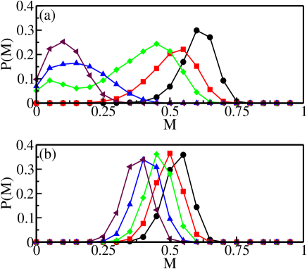
Figure 6: (color online) Plot of PDF of order parameter $P(M)$ for $\gamma=0$ where the black (circle), red (square), green (diamond), blue (triangle left) and maroon (triangle up) symbols represents the temperatures (a) $T=2.15$, $T=2.20$, $T=2.25$, $T=2.30$ and $T=2.35$ respectively and (b) $T=1.65$, $T=1.70$, $T=1.75$ $T=1.80$ and $T=1.85$ respectively near the disorder-to-order transition. Lines are guide to eyes.

IV Coarse-grained hydrodynamic equations of motion

Now we introduce the coarse-grained hydrodynamic equations of motion for slow variables: density $\rho({\bf r},t)$ and polarisation order parameter ${\bf P}({\bf r},t)$. Former is globally conserved and later is nonzero for the broken symmetry state. The equation of motion for local density field $\rho({\bf r},t)$

$$\frac{\partial\rho}{\partial t}=-v_{0}\nabla.({\bf P}\rho)+D_{\rho}\nabla^{2}\rho+\gamma g({\rho})$$ (3)

The hydrodynamic equation of motion for the local polarisation ${\bf P}({\bf r},t)$,

$$\frac{\partial{\bf P}}{\partial t}=(\alpha_{1}(\rho)-\alpha_{2}\mid{\bf P}\mid^{2}){\bf P}-v_{1}\nabla\rho+\lambda({\bf P}\cdot\nabla{\bf P})+D\nabla^{2}{\bf P}$$ (4)

Equation (3) represents continuity equation with additional birth and death term $g(\rho)=\rho(\rho-\rho_{0})$ for the density field $\rho$. Where $\rho_{0}$ is the mean density of particles in the system. $\gamma$ is the birth and death rate. The first term on the right hand side of Eq. 3, describes the convection due to self-propulsion velocity $v_{0}\bf P$. The second term on the right hand side of Eq. 3 is diffusion due to density gradient. In polarisation ${\bf P}({\bf r},t)$, Eq. (4), the first term on right hand side represents a mean field transition from an isotropic state ($\bf P=0$) to a broken symmetry state ${\bf P}=\sqrt{\frac{\alpha_{1}(\rho_{0})}{\alpha_{2}}}{\bf\hat{x}}$ (the direction of broken symmetry is chosen along $x-$axis). The second and third term indicate hydrostatic pressure due to density gradient and convection in the model, respectively. Both $\lambda$ and $v_{1}$ depends on self-propelled speed of the particle Bertin et al. (2006). The fourth term represents diffusion in the polarisation field. The above two equations are similar to the equations introduced in Toner and Tu (1998a). Here we introduced an additional term due to birth and death in the density equation. We first analyse the equations for the broken symmetry or the ordered homogeneous state of the two Eqs. 3 and 4, $\rho=\rho_{0}$ and ${\bf P}=P_{0}=\sqrt{\frac{\alpha_{1}(\rho_{0})}{\alpha_{2}}}\hat{\bf x}$. We further add small perturbation on the above homogeneous ordered state and write: $\rho=\rho_{0}+\delta\rho({\bf r},t)$ and ${\bf P}=(P_{0}+\delta P_{x})\hat{x}+\delta P_{y}\hat{y}$. $\delta\rho({\bf r},t)$, $\delta P_{x}({\bf r},t)$ and $\delta P_{y}({\bf r},t)$ are the fluctuations in the density, longitudinal and transverse directions of polarisation respectively. Since system shows a mean-field transition from disordered-to-ordered state where $\alpha_{1}$, changes sign. Hence at the transition point $\alpha_{1}=0$. We take $\alpha_{1}=0$ (at the mean-field transition point) and substitute for the $\rho$ and ${\bf P}$ from the above expressions and further write the Eqs. 3 and 4 for the small fluctuations $\delta\rho,\delta P_{x},\delta P_{y}$ to the linear order. The equation for $\delta P_{x}$, will not contribute to linear order. Hence only the equations for the local density fluctuation $\delta\rho({\bf r},t)$ and local transverse polarisation fluctuation $\delta P_{y}({\bf r},t)$ will survive. We further take the Fourier transform of the two equations using ${\bf A}({\bf q},\omega)=\int{{\bf A}({\bf r},t)\exp(i{\bf q}\cdot{\bf r}+i\omega t)d{\bf r}d\omega}$, where ${\bf A}=(\delta\rho,\delta P_{y})$. Hence the two equations will become:

$$(-i\omega+D_{\rho}q^{2}+\gamma\rho_{0})\delta\rho+iq_{y}v_{0}\rho_{0}\delta P_{y}=0$$ (5)

and

$$iq_{y}\frac{v_{1}}{2\rho_{0}}\delta\rho+(-i\omega+Dq^{2})\delta P_{y}=0$$ (6)

where the wavevector $q$ is in the direction of broken symmetry. We further do the analysis for the transverse direction $q_{y}=q$. We further write the above two Eqs. 5 and 6 in matrix notation and solve for the two modes $\omega_{\pm}$ using the determinant of the matrix and find the two modes as

$$\omega_{\pm}=\frac{-i\gamma\rho_{0}}{2}\pm\frac{iq}{2}\sqrt{2v_{0}v_{1}+2\gamma\rho_{0}(D_{\rho}-D)}$$ (7)

We further use the solution for the two modes to performed the renormalised mean-field study of the system in the isotropic state. In the next section we carry out the perturbative study of the hydrodynamic equations about the isotropic state.

IV.1 Perturbative renormalised mean-field study in the isotropic state

We additionally introduce small fluctuations about the isotropic state; $\rho=\rho_{0}+\delta\rho$ and ${\bf P}=(\delta P_{x},\delta P_{y})$ and write the equations for the small fluctuations $\delta\rho$ and $\delta{\bf P}=(\delta P_{x},\delta P_{y})$. The solution for the Fourier transformed local density fluctuation $\delta\rho({\bf q},\omega)$ and polarisation fluctuations $\delta{\bf P}({\bf q},\omega)$ will become;

$$\delta\rho({\bf q},\omega)={} \ \frac{-v_{0}\rho_{0}i{\bf q}.{\delta{\bf P}({\bf q},\omega)}}{(-i\omega+D_{\rho}q^{2}+\gamma\rho_{0})}$$ (8)

$$\ -\frac{1}{2}\frac{v_{0}i{\bf q}.\displaystyle\int{[\delta P({\bf k},\Omega)\delta\rho({{\bf q}-{\bf k}},\omega-\Omega)+\delta P({{\bf q}-{\bf k}},\omega-\Omega)\delta\rho(k,\omega)]d{\bf k}d\Omega}}{(-i\omega+D_{\rho}q^{2}+\gamma\rho_{0})}$$

and

$$-i\omega\delta{\bf P}({\bf q},\omega)={} \-\alpha_{1}(\rho_{0})\delta{\bf P}({\bf q},\omega)$$ (9)

$$\ +{\alpha_{1}}^{\prime}(\rho_{0})\frac{1}{2}\left[\int{\delta{\bf P}({\bf k},\Omega)\delta\rho({\bf q}-{\bf k},\omega-\Omega)+\delta{\bf P}({\bf q}-{\bf k}},\omega-\Omega)\delta\rho({\bf k},\Omega)d{\bf k}d\Omega\right]$$

$$\ -\alpha_{2}\int{\delta{\bf P}({\bf k},\Omega)\delta{\bf P}({\bf k^{\prime}},\Omega-\Omega^{\prime})\delta{\bf P}({\bf q}-{\bf k}-{\bf k}^{\prime},\omega-\Omega-\Omega^{\prime})d{\bf k}d{\bf k^{\prime}}d\Omega d\Omega}$$

Here we write only first two terms in the polarisation Eq. 4. $\alpha_{1}^{\prime}(\rho_{0})=\frac{\partial{\alpha_{1}}}{\partial\rho}\Big{|}_{\rho=\rho_{0}}$. Substitute for $\delta\rho$ leading order from Eq. 8 and substituting for one of mode $\omega_{+}$ from Eq. 7

$$-i\omega\delta{\bf P}({\bf q},\omega)={} \ \alpha_{1}(\rho_{0})\delta{\bf P}({\bf q},\omega)$$ (10)

$$\ +\frac{1}{2}{\alpha_{1}}^{\prime}(\rho_{0})\Bigg{[}\frac{\int(\delta{\bf P}({\bf k})(v_{0}\rho_{0}({\bf q}-{\bf k}))\delta{\bf P}({\bf q}-{\bf k},\omega-\Omega))}{6\gamma\rho_{0}+(q-k)\sqrt{2v_{0}v_{1}+\gamma\rho_{0}(D_{\rho}-D)}}$$

$$\ +\frac{\int(\delta{\bf P}({\bf q}-{\bf k},\omega-\Omega)(v_{0}\rho_{0}{\bf k})\delta P({\bf k},\Omega))}{\gamma\rho_{0}+k\sqrt{2v_{0}v_{1}+\gamma\rho_{0}(D_{\rho}-D)}}\Bigg{]}$$

$$\ -\alpha_{2}\int{\delta{\bf P}({\bf k},\Omega)\delta{\bf P}({\bf k^{\prime}},\Omega-\Omega^{\prime})\delta{\bf P}({\bf q}-{\bf k}-{\bf k}^{\prime},\omega-\Omega-\Omega^{\prime})d{\bf k}d{\bf k^{\prime}}d\Omega d\Omega}$$

It is complicated to solve the above equation for the dimensions $d=2$, when $\delta{\bf P}$ is a vector. However the usual flocking transition is characterised by the appearance of bands near the transition Chaté et al. (2008); Solon and Tailleur (2013); Bhattacherjee et al. (2015). When bands form, the local density and polarisation shows the variation only along the direction of moving bands and in the transverse direction it is homogeneous both in space and time. Hence system can be considered one dimensional where both $\delta{\bf P}$ and $\delta\rho$, only vary along the direction of moving bands. And all the vectors can be replaced by scalars in Eqs. 10. In such conditions, we can rewrite the above Eq. 10 as

$$-i\omega\delta P({\bf q},\omega)={} \ \alpha_{1}(\rho_{0})\delta P(q,\omega)$$ (11)

$$\ +\frac{1}{2}\alpha_{1}^{\prime}(\rho_{0})\bigg{[}\frac{v_{0}\rho_{0}\int{\delta P(q-k,\omega-\Omega)(q-k)\delta P(k,\Omega)dkd\Omega}}{6\gamma\rho_{0}+(q-k)\sqrt{2v_{0}v_{1}+\gamma\rho_{0}(D_{\rho}-D)}}$$

$$\ +\frac{v_{0}\rho_{0}\int{\delta P(q-k,\omega-\Omega)k\delta P(k,\Omega)dkd\Omega}}{6\gamma\rho_{0}+k\sqrt{2v_{0}v_{1}+\gamma\rho_{0}(D_{\rho}-D)}}\bigg{]}$$

$$\ -\alpha_{2}\int{\delta P(k,\Omega)\delta P(k^{\prime},\Omega^{\prime})\delta P(q-k-k^{\prime},\omega-\Omega-\Omega^{\prime})dkdk^{\prime}d\Omega d\Omega^{\prime}}$$

Case with no birth and death ($\gamma=0$):
Now for the zero $\gamma$ or no birth and death, we write the effective free energy $\mathcal{F}_{eff}(\delta P)$ using Eq. 11 as

$$\mathcal{F}_{eff}(\delta P)={} \ -\alpha_{1}(\rho_{0})\int{dk\frac{\delta P(k)\delta P(q-k)}{2}}$$ (12)

$$\ -\frac{\alpha_{1}^{\prime}(\rho_{0})}{6}\sqrt{\frac{v_{0}}{2v_{1}}}\int{dkdk^{\prime}\left[\delta P(k)\delta P(q-k-k^{\prime})\delta P(k^{\prime})\right]}$$

$$\ +\alpha_{2}\frac{1}{4}\int{dkdk^{\prime}dk^{\prime\prime}\delta P(k)\delta P(k^{\prime})\delta P(k^{\prime\prime})\delta P(q-k-k^{\prime}-k^{\prime\prime})}$$

Taking the inverse Fourier transform, the expression for the $\mathcal{F}_{eff}({\delta P})$ and assuming the homogeneous $\delta P$. The effective free energy $\mathcal{F}_{eff}(\delta P)$ is real space will become

$$\mathcal{F}_{eff}(\delta P)=-\alpha_{1}(\rho_{0})\frac{\delta P^{2}}{2}-\frac{\alpha_{1}^{\prime}(\rho_{0})}{6}\sqrt{\frac{v_{0}}{2v_{1}}}\delta P^{3}+\frac{\alpha_{2}}{4}\delta P^{4}$$ (13)

Hence for the zero birth and death, the second term of the right hand side is an additional expression which is cubic order in $\mathcal{O}(\delta P^{3})$. The presence of such nonlinear term can leads the mean-field transition to first order. Now we examine the system for finite $\gamma$, using the denominator of Eq. 11

$$\gamma\rho_{0}\gg\frac{q\sqrt{2v_{0}v_{1}+\gamma\rho_{0}(D_{\rho}-D)}}{6}$$ (14)

Then, the second term in Eq. 10 will be of the form $P\nabla P$ and this term can be compared with the convective nonlinear term of the type ${\bf P}\cdot\nabla{\bf P}$ in the hydrodynamic Eq. 4. After solving Eq. 14 for $\gamma$ we get,

$$\gamma>\frac{q\Delta D}{72\rho_{0}}(1+\sqrt{q^{2}+\frac{288v_{0}v_{1}}{\Delta D}^{2}})$$ (15)

where $\Delta D=|D_{\rho}-D|$. Hence if $\gamma$ is greater than the right hand side of Eq. 15, the birth and death term will dominate and transition will be of type as predicted by mean field theory, whereas for finite and small $\gamma$ such that

$$\gamma\rho_{0}\ll\frac{q\sqrt{2v_{0}v_{1}+\gamma\rho_{0}(D_{\rho}-D)}}{6}$$ (16)

the effective free energy for $\mathcal{F}_{eff}(\delta P)$ will become

$$F_{eff}(\delta P)={} \ -\frac{1}{2}\alpha_{1}(\rho_{0})\delta P^{2}+$$ (17)

$$\ -\frac{v_{0}\rho_{0}\alpha_{1}^{\prime}(\rho_{0})\delta P^{3}}{6\sqrt{2v_{0}v_{1}+\gamma\rho_{0}(D_{\rho}-D)}}+\frac{\alpha_{2}}{4}\delta P^{3}$$

Hence for small $\gamma$, the wavevector dependence of additional convective non-linear term in Eq. 11 goes away and it contributes an additional $\mathcal{O}(\delta P^{3})$ nonlinearity in the effective free energy. Which will lead the transition to discontinuous type or first order. Hence the first order or discontinuous transition happens through the competition of a length scale and birth and death rate as given in Eq. 15. For large wavevector $q$ (or small wavelength) term on the right hand side of Eq. 15, larger $\gamma$ will make the transition continuous type and vice versa. Hence the wavelength ($q^{-1}$) of the density and magnetisation fluctuations decreases with increasing birth and death term. As shown in Fig. 4, on increasing $\gamma$ from $\gamma=0$, the bands start to split and their size deceases, and the nature of transition becomes more and more continuous type as predicted by mean-field type.

We further analysed the properties of effective free energy in the presence of additional cubic order nonlinearity. In simplified notation the effective free energy can be written as

$$\mathcal{F}(\delta P)=-\beta_{1}\delta P^{2}-\beta_{2}\delta P^{3}+\beta_{3}\delta P^{4}$$ (18)

where $\beta_{1}=\frac{1}{2}\alpha_{1}(\rho_{0})$, $\beta_{2}=\frac{v_{0}\rho_{0}\alpha_{1}^{\prime}(\rho_{0})}{6\sqrt{2v_{0}v_{1}+\gamma\rho_{0}(D_{\rho}-D)}}$, $\beta_{3}=\frac{\alpha_{2}}{4}$. For the transition to be first order we impose the coexistence condition i.e. $\mathcal{F}(\delta P=0)=\mathcal{F}(\delta P\neq 0)$, that gives

$$-\beta_{1}-\beta_{2}\delta P+\beta_{3}\delta P^{2}=0$$ (19)

also the condition of steady state implies $\frac{\partial\mathcal{F}}{\partial\delta P}=0$

$$-2\beta_{1}-3\beta_{2}\delta P+4\beta_{3}\delta P^{2}=0$$ (20)

using Eq. 19 and 20 the jump in the order parameter $P$ at the transition

$$\delta P=\frac{\mid\beta_{2}\mid}{2\beta_{3}}$$ (21)

and the jump is always positive, hence the finite jump. Putting the value of $\delta P$ in Eq. 19 and solve for $\beta_{1}$, $\beta_{1}-\frac{\beta_{2}^{2}}{4\beta_{3}}=0$. We get $\beta_{1}^{c}=\frac{\beta_{2}^{2}}{4\beta_{3}}$ again a positive term. We further analyse the jump in the order parameter and transition point using $\beta_{2}=\frac{v_{0}\rho_{0}\alpha_{1}^{\prime}(\rho_{0})}{6\sqrt{2v_{0}v_{1}+\gamma\rho_{0}\vartriangle D}}$ and $\delta P=\frac{4v_{0}\rho_{0}\alpha_{1}^{\prime}(\rho_{0})}{3\alpha_{3}\sqrt{2v_{0}v_{1}+\gamma\rho_{0}\vartriangle D}}$. Assuming the temperature dependence of $\alpha_{1}$ in the mean-field theory $\alpha_{1}(\rho,T)=\alpha_{0}(\rho)(T-T^{*})$, $T^{*}$ is point where there is a mean-field type second order phase transition for large $\gamma$. Hence if we define the true critical temperature as $T_{c}$, where $\beta_{1}=\frac{\beta_{2}^{2}}{4\beta_{3}}$, and at the critical point $\alpha_{1}^{c}(\rho,T)=\alpha_{0}(\rho)(T_{c}-T^{*})=2\beta_{1}$ $\>0$. Hence we find that $T_{c}>T^{*}$ and $T_{c}=\frac{\beta_{2}^{2}}{2\beta_{3}\alpha_{0}}+T^{*}$. After substituting the value of $\beta_{2}$ and $\beta_{3}$ from the previous expressions, we find $T_{c}=T^{*}+\frac{2{v_{0}}^{2}{\rho_{0}}^{2}{{\alpha_{0}}^{\prime}}^{2}\rho_{0}}{9(2v_{0}v_{1}+\gamma\rho_{0}\vartriangle D)\alpha_{2}\alpha_{0}(\rho_{0})}$. Hence in the simplified notation we can write $T_{c}=T^{*}+\frac{A}{B+\gamma}$ where $A=\frac{4{v_{0}}^{2}{\rho_{0}}^{2}{{\alpha_{0}}^{\prime}}^{2}\rho_{0}}{9\rho_{0}\Delta D\alpha_{3}\alpha_{0}(\rho_{0})}$ and $B=\frac{2v_{0}v_{1}}{\rho_{0}\Delta D}$. For large $\gamma$, second term in the expression for $T_{c}$ is negligible and critical point happens at $T^{*}$. As we start tuning $\gamma$ towards lower values, the phase transition shift towards right as obtained in our numerical study Fig. 2. Also $\delta P$, (the jump in order parameter) is almost zero for large $\gamma$ that means system approaches critical point continuously as found in our numerical study Fig. 6(b). But as we start decreasing $\gamma$ transition happens with a finite jump in order parameter Fig. 6(a).

V Discussion

We studied a system of active Ising spins with the presence of birth and death on a two dimensional substrate with periodic boundary condition. The system is studied using Metropolis-Monte -Carlo for the interaction among the spins and the spin perform the biased move along their direction of orientation. System is studied for fixed activity and varying birth and death rate $\gamma$. Its shows a phase transition from disorder-to-order for all $\gamma$ and fixed activity on varying temperature from high to low. The transition is of first order discontinuous type for conserved model ($\gamma=0$) and becomes continuous type for the birth and death model. Also transition shifts towards higher temperature on decreasing $\gamma$. Hence the presence of birth and death rate tune the disorder-to-order transition to lower temperature and shows a crossover from discontinuous to continuous type in the polar flock. The results are verified with the help of coarse-grained hydrodynamic equations of motion for local density and polarisation in the presence of birth and death.
Hence our study shows effect of birth and death on the nature of phase transition of polar-flock. The present model is studied for discrete Ising spins with the Globular conserved model Binder et al. (2000) for the spin interaction. It is worth to study the system for the non-conserved Kawasaki type Binder (1987) of spin interaction as well for the off-lattice systems.

Acknowledgement : SM, thanks J K Bhattacharjee for useful discussion at the start of the project. SM also thanks S. Ramaswamy and M. C. Marchetti for introducing the problem a few years back. SM and PKM, thanks PARAM Shivay for computatational facility under the National Supercomputing Mission, Government of India at the Indian Institute of Technology, Varanasi. Computing facility at Indian Institute of Technology(BHU), Varanasi is gratefully acknowledged.

References

- Toner et al. (2005) J. Toner, Y. Tu, and S. Ramaswamy, Annals of Physics 318, 170 (2005), special Issue.
- Toner and Tu (1995) J. Toner and Y. Tu, Phys. Rev. Lett. 75, 4326 (1995).
- Toner and Tu (1998a) J. Toner and Y. Tu, Phys. Rev. E 58, 4828 (1998a).
- Toner and Tu (1998b) J. Toner and Y. Tu, Phys. Rev. E 58, 4828 (1998b).
- Bechinger et al. (2016) C. Bechinger, R. Di Leonardo, H. Löwen, C. Reichhardt, G. Volpe, and G. Volpe, Rev. Mod. Phys. 88, 045006 (2016).
- Vicsek and Zafeiris (2012) T. Vicsek and A. Zafeiris, Physics Reports 517, 71 (2012).
- Gompper et al. (2020) G. Gompper, R. G. Winkler, and S. Kale, Journal of Physics: Condensed Matter 32, 193001 (2020).
- Saintillan (2010) D. Saintillan, Phys. Rev. E 81, 056307 (2010).
- Shen and Wolynes (2004) T. Shen and P. G. Wolynes, Proceedings of the National Academy of Sciences 101, 8547 (2004), https://www.pnas.org/content/101/23/8547.full.pdf .
- Dombrowski et al. (2004) C. Dombrowski, L. Cisneros, S. Chatkaew, R. E. Goldstein, and J. O. Kessler, Phys. Rev. Lett. 93, 098103 (2004).
- Kemkemer et al. (2000) R. Kemkemer, D. Kling, D. Kaufmann, and H. Gruler, European Physical Journal E 1, 215 (2000).
- Surrey et al. (2001) T. Surrey, F. Nédélec, S. Leibler, and E. Karsenti, Science 292, 1167 (2001).
- Bendix et al. (2008) P. Bendix, G. Koenderink, D. Cuvelier, Z. Dogic, B. Koeleman, W. Brieher, C. Field, L. Mahadevan, and D. Weitz, Biophysical Journal 94, 3126 (2008).
- Chaté et al. (2008) H. Chaté, F. Ginelli, G. Grégoire, and F. Raynaud, Phys. Rev. E 77, 046113 (2008).
- Buttinoni et al. (2013) I. Buttinoni, J. Bialk’e, F. Kümmel, H. Löwen, C. Bechinger, and T. Speck, Physical review letters 110 23, 238301 (2013).
- Bhattacherjee et al. (2015) B. Bhattacherjee, S. Mishra, and S. S. Manna, Phys. Rev. E 92, 062134 (2015).
- Pattanayak and Mishra (2018) S. Pattanayak and S. Mishra, Journal of Physics Communications 2, 045007 (2018), arXiv:1803.11368 [cond-mat.stat-mech] .
- Singh et al. (2021) J. P. Singh, S. Kumar, and S. Mishra, Journal of Statistical Mechanics: Theory and Experiment 2021, 083217 (2021).
- Durve and Sayeed (2016) M. Durve and A. Sayeed, Phys. Rev. E 93, 052115 (2016).
- Giomi et al. (2010) L. Giomi, T. B. Liverpool, and M. C. Marchetti, Phys. Rev. E 81, 051908 (2010).
- Ramaswamy et al. (2003) S. Ramaswamy, R. A. Simha, and J. Toner, Europhysics Letters (EPL) 62, 196 (2003).
- Solon and Tailleur (2013) A. P. Solon and J. Tailleur, Phys. Rev. Lett. 111, 078101 (2013).
- Solon and Tailleur (2015) A. P. Solon and J. Tailleur, Phys. Rev. E 92, 042119 (2015).
- Vicsek et al. (1995) T. Vicsek, A. Czirók, E. Ben-Jacob, I. Cohen, and O. Shochet, Phys. Rev. Lett. 75, 1226 (1995).
- Kolmogorov (1936) A. N. Kolmogorov, Math. Ann. 112, 155 (1936).
- (26) The mutual exclusion help us to introduce birth and death in simple manner (which we explain later) .
- Ising (1925) E. Ising, Zeitschrift fur Physik 31, 253 (1925).
- Landau and Binder (2005) D. P. Landau and K. Binder, “Frontmatter,” in A Guide to Monte Carlo Simulations in Statistical Physics (Cambridge University Press, 2005) pp. i–iv, 2nd ed.
- Pathria and Beale (2011) R. Pathria and P. D. Beale, in Statistical Mechanics (Third Edition), edited by R. Pathria and P. D. Beale (Academic Press, Boston, 2011) third edition ed., pp. 39–90.
- Mishra et al. (2010) S. Mishra, A. Baskaran, and M. C. Marchetti, Phys. Rev. E 81, 061916 (2010).
- Bertin et al. (2006) E. Bertin, M. Droz, and G. Grégoire, Phys. Rev. E 74, 022101 (2006).
- Binder et al. (2000) K. Binder, E. Luijten, M. Müller, N. B. Wilding, and H. W. J. Blöte, Physica A Statistical Mechanics and its Applications 281, 112 (2000), arXiv:cond-mat/9908270 [cond-mat.stat-mech] .
- Binder (1987) K. Binder, “Applications of the Monte Carlo Method in Statistical Physics,” Applications of the Monte Carlo Method in Statistical Physics. Series: Topics in Current Physics (1987).