Patches Are All You Need?

Abstract

Although convolutional networks have been the dominant architecture for vision tasks for many years, recent experiments have shown that Transformer-based models, most notably the Vision Transformer (ViT), may exceed their performance in some settings. However, due to the quadratic runtime of the self-attention layers in Transformers, ViTs require the use of patch embeddings, which group together small regions of the image into single input features, in order to be applied to larger image sizes. This raises a question: Is the performance of ViTs due to the inherently-more-powerful Transformer architecture, or is it at least partly due to using patches as the input representation? In this paper, we present some evidence for the latter: specifically, we propose the ConvMixer, an extremely simple model that is similar in spirit to the ViT and the even-more-basic MLP-Mixer in that it operates directly on patches as input, separates the mixing of spatial and channel dimensions, and maintains equal size and resolution throughout the network. In contrast, however, the ConvMixer uses only standard convolutions to achieve the mixing steps. Despite its simplicity, we show that the ConvMixer outperforms the ViT, MLP-Mixer, and some of their variants for similar parameter counts and data set sizes, in addition to outperforming classical vision models such as the ResNet. Our code is available at https://github.com/locuslab/convmixer.

1 Introduction

Figure 1: Accuracy vs. parameters, trained and evaluated on ImageNet-1k.

For many years, convolutional neural networks have been the dominant architecture for deep learning systems applied to computer vision tasks. But recently, architectures based upon Transformer models, e.g., the so-called Vision Transformer architecture (Dosovitskiy et al., 2020), have demonstrated compelling performance in many of these tasks, often outperforming classical convolutional architectures, especially for large data sets. An understandable assumption, then, is that it is only a matter of time before Transformers become the dominant architecture for vision domains, just as they have for language processing. In order to apply Transformers to images, however, the representation had to be changed: because the computational cost of the self-attention layers used in Transformers would scale quadratically with the number of pixels per image if applied naively at the per-pixel level, the compromise was to first split the image into multiple “patches”, linearly embed them, and then apply the transformer directly to this collection of patches.

In this work, we explore the question of whether, fundamentally, the strong performance of vision transformers may result more from this patch-based representation than from the Transformer architecture itself. We develop a very simple convolutional architecture which we dub the “ConvMixer” due to its similarity to the recently-proposed MLP-Mixer (Tolstikhin et al., 2021). This architecture is similar to the Vision Transformer (and MLP-Mixer) in many respects: it directly operates on patches, it maintains an equal-resolution-and-size representation throughout all layers, it does no downsampling of the representation at successive layers, and it separates “channel-wise mixing” from the “spatial mixing” of information. But unlike the Vision Transformer and MLP-Mixer, our architecture does all these operations via only standard convolutions.

The chief result we show in this paper is that this ConvMixer architecture, despite its extreme simplicity (it can be implemented in $\approx 6$ lines of dense PyTorch code), outperforms both “standard” computer vision models such as ResNets of similar parameter counts and some corresponding Vision Transformer and MLP-Mixer variants, even with a slate of additions intended to make those architectures more performant on smaller data sets. Importantly, this is despite the fact that we did not design our experiments to maximize accuracy nor speed, in contrast to the models we compared against. Our results suggest that, at least to some extent, the patch representation itself may be a critical component to the “superior” performance of newer architectures like Vision Transformers. While these results are naturally just a snapshot, and more experiments are required to exactly disentangle the effect of patch embeddings from other factors, we believe that this provides a strong “convolutional-but-patch-based” baseline to compare against for more advanced architectures in the future.

2 A Simple Model: ConvMixer

Our model, dubbed ConvMixer, consists of a patch embedding layer followed by repeated applications of a simple fully-convolutional block. We maintain the spatial structure of the patch embeddings, as illustrated in Fig. 2. Patch embeddings with patch size $p$ and embedding dimension $h$ can be implemented as convolution with $c_{\mathsf{in}}$ input channels, $h$ output channels, kernel size $p$, and stride $p$:

$$z_{0}=\mathsf{BN}\left(\sigma\{\text{{Conv}}_{c_{\mathsf{in}}\to h}(X,\text{{stride=}}p,\text{{kernel\_size}=}p)\}\right)$$ (1)

The ConvMixer block itself consists of depthwise convolution (i.e., grouped convolution with groups equal to the number of channels, $h$) followed by pointwise (i.e., kernel size $1\times 1$) convolution. As we will explain in Sec. 3, ConvMixers work best with unusually large kernel sizes for the depthwise convolution. Each of the convolutions is followed by an activation and post-activation BatchNorm:

$$z_{l}^{\prime} =\mathsf{BN}\left(\sigma\{\text{{ConvDepthwise}}(z_{l-1})\}\right)+z_{l-1}$$ (2)

$$z_{l+1} =\mathsf{BN}\left(\sigma\{\text{{ConvPointwise}}(z_{l}^{\prime})\}\right)$$ (3)

After many applications of this block, we perform global pooling to get a feature vector of size $h$, which we pass to a softmax classifier. See Fig. 3 for an implementation of ConvMixer in PyTorch.

Figure 2: ConvMixer uses “tensor layout” patch embeddings to preserve locality, and then applies $d$ copies of a simple fully-convolutional block consisting of large-kernel depthwise convolution followed by pointwise convolution, before finishing with global pooling and a simple linear classifier.

⬇

def ConvMixer(h, depth, kernel_size=9, patch_size=7, n_classes=1000):

Seq, ActBn = nn.Sequential, lambda x: Seq(x, nn.GELU(), nn.BatchNorm2d(h))

Residual = type(’Residual’, (Seq,), {’forward’: lambda self, x: self[0](x) + x})

return Seq(ActBn(nn.Conv2d(3, h, patch_size, stride=patch_size)),

*[Seq(Residual(ActBn(nn.Conv2d(h, h, kernel_size, groups=h, padding=”same”))),

ActBn(nn.Conv2d(h, h, 1))) for i in range(depth)],

nn.AdaptiveAvgPool2d((1,1)), nn.Flatten(), nn.Linear(h, n_classes))

Figure 3: Implementation of ConvMixer in PyTorch; see Appendix D for more implementations.

Design parameters. An instantiation of ConvMixer depends on four parameters: (1) the “width” or hidden dimension $h$ (i.e., the dimension of the patch embeddings), (2) the depth $d$, or the number of repetitions of the ConvMixer layer, (3) the patch size $p$ which controls the internal resolution of the model, (4) the kernel size $k$ of the depthwise convolutional layer. We name ConvMixers after their hidden dimension and depth, like ConvMixer-$h/d$. We refer to the original input size $n$ divided by the patch size $p$ as the internal resolution; note, however, that ConvMixers support variable-sized inputs.

Motivation. Our architecture is based on the idea of mixing, as in Tolstikhin et al. (2021). In particular, we chose depthwise convolution to mix spatial locations and pointwise convolution to mix channel locations. A key idea from previous work is that MLPs and self-attention can mix distant spatial locations, i.e., they can have an arbitrarily large receptive field. Consequently, we used convolutions with an unusually large kernel size to mix distant spatial locations.

While self-attention and MLPs are theoretically more flexible, allowing for large receptive fields and content-aware behavior, the inductive bias of convolution is well-suited to vision tasks and leads to high data efficiency. By using such a standard operation, we also get a glimpse into the effect of the patch representation itself in contrast to the conventional pyramid-shaped, progressively-downsampling design of convolutional networks.

Current “Most Interesting” ConvMixer Configurations vs. Other Simple Models
Network	Patch Size	Kernel Size	# Params ($\times 10^{6}$)	Throughput (img/sec)	Act. Fn.	# Epochs	ImNet top-1 (%)
ConvMixer-1536/20	7	9	51.6	134	G	150	81.37
ConvMixer-768/32	7	7	21.1	206	R	300	80.16
ResNet-152	–	3	60.2	828	R	150	79.64
DeiT-B	16	–	86	792	G	300	81.8
ResMLP-B24/8	8	–	129	181	G	400	81.0

Table 1: Models trained and evaluated on $224\times 224$ ImageNet-1k only. See more in Appendix A.

3 Experiments

Training setup. We primarily evaluate ConvMixers on ImageNet-1k classification without any pretraining or additional data. We added ConvMixer to the timm framework (Wightman, 2019) and trained it with nearly-standard settings: we used RandAugment (Cubuk et al., 2020), mixup (Zhang et al., 2017), CutMix (Yun et al., 2019), random erasing (Zhong et al., 2020), and gradient norm clipping in addition to default timm augmentation. We used the AdamW (Loshchilov & Hutter, 2018) optimizer and a simple triangular learning rate schedule. Due to limited compute, we did absolutely no hyperparameter tuning on ImageNet and trained for fewer epochs than competitors. Consequently, our models could be over- or under-regularized, and the accuracies we report likely underestimate the capabilities of our model.

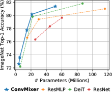
Results. A ConvMixer-1536/20 with 52M parameters can achieve 81.4% top-1 accuracy on ImageNet, and a ConvMixer-768/32 with 21M parameters 80.2% (see Table 1). Wider ConvMixers seem to converge in fewer epochs, but are memory- and compute-hungry. They also work best with large kernel sizes: ConvMixer-1536/20 lost $\approx 1\%$ accuracy when reducing the kernel size from $k=9$ to $k=3$ (we discuss kernel sizes more in Appendix A & B). ConvMixers with smaller patches are substantially better in our experiments, similarly to Sandler et al. (2019); we believe larger patches require deeper ConvMixers. With everything held equal except increasing the patch size from 7 to 14, ConvMixer-1536/20 achieves 78.9% top-1 accuracy but is around 4$\times$ faster. We trained one model with ReLU to demonstrate that GELU (Hendrycks & Gimpel, 2016), which is popular in recent isotropic models, isn’t necessary.

Comparisons. Our model and ImageNet1k-only training setup closely resemble that of recent patch-based models like DeiT (Touvron et al., 2020). Due to ConvMixer’s simplicity, we focus on comparing to only the most basic isotropic patch-based architectures adapted to the ImageNet-1k setting, namely DeiT and ResMLP. Attempting a fair comparison with a standard baseline, we trained ResNets using exactly the same parameters as ConvMixers; while this choice of parameters is suboptimal (Wightman et al., 2021), it is likely also suboptimal for ConvMixers, since we did no hyperparameter tuning.

Looking at Table 1 and Fig. 1, ConvMixers achieve competitive accuracies for a given parameter budget: ConvMixer-1536/20 outperforms both ResNet-152 and ResMLP-B24 despite having substantially fewer parameters and is competitive with DeiT-B. ConvMixer-768/32 uses just a third of the parameters of ResNet-152, but is similarly accurate. Note that unlike ConvMixer, the DeiT and ResMLP results involved hyperparameter tuning, and when substantial resources are dedicated to tuning ResNets, including training for twice as many epochs, they only outperform an equivalently-sized ConvMixer by $\approx 0.2\%$ (Wightman et al., 2021). However, ConvMixers are substantially slower at inference than the competitors, likely due to their smaller patch size; hyperparameter tuning and optimizations could narrow this gap. For more discussion and comparisons, see Table 2 and Appendix A.

Hyperparameters. For experiments presented in the main text, we used only one set of “common sense” parameters for the regularization methods. Recently, we adapted parameters from the A1 procedure in Wightman et al. (2021), published after our work, which were better than our initial guess, e.g., giving $+0.8\%$ for ConvMixer-1536/20, or 82.2% top-1 accuracy (see Appendix A).

CIFAR-10 Experiments. We also performed smaller-scale experiments on CIFAR-10, where ConvMixers achieve over 96% accuracy with as few as 0.7M parameters, demonstrating the data efficiency of the convolutional inductive bias. Details of these experiments are presented in Appendix B.

4 Related Work

Isotropic architectures. Vision transformers have inspired a new paradigm of “isotropic” architectures, i.e., those with equal size and shape throughout the network, which use patch embeddings for the first layer. These models look similar to repeated transformer-encoder blocks (Vaswani et al., 2017) with different operations replacing the self-attention and MLP operations. For example, MLP-Mixer (Tolstikhin et al., 2021) replaces them both with MLPs applied across different dimensions (i.e., spatial and channel location mixing); ResMLP (Touvron et al., 2021a) is a data-efficient variation on this theme. CycleMLP (Chen et al., 2021), gMLP (Liu et al., 2021a), and vision permutator (Hou et al., 2021), replace one or both blocks with various novel operations. These are all quite performant, which is typically attributed to the novel choice of operations. In contrast, Melas-Kyriazi (2021) proposed an MLP-based isotropic vision model, and also hypothesized patch embeddings could be behind its performance. ResMLP tried replacing its linear interaction layer with (small-kernel) convolution and achieved good performance, but kept its MLP-based cross-channel layer and did not explore convolutions further. As our investigation of ConvMixers suggests, these works may conflate the effect of the new operations (like self-attention and MLPs) with the effect of the use of patch embeddings and the resulting isotropic architecture.

A study predating vision transformers investigate isotropic (or “isometric”) MobileNets (Sandler et al., 2019), and even implements patch embeddings under another name. Their architecture simply repeats an isotropic MobileNetv3 block. They identify a tradeoff between patch size and accuracy that matches our experience, and train similarly performant models (see Appendix A, Table 2). However, their block is substantially more complex than ours; simplicity and motivation sets our work apart.

Patches aren’t all you need. Several papers have increased vision transformer performance by replacing standard patch embeddings with a different stem: Xiao et al. (2021) and Yuan et al. (2021a) use a standard convolutional stem, while Yuan et al. (2021b) repeatedly combines nearby patch embeddings. However, this conflates the effect of using patch embeddings with the effect of adding convolution or similar inductive biases e.g., locality. We attempt to focus on the use of patches.

CNNs meet ViTs. Many efforts have been made to incorporate features of convolutional networks into vision transformers and vice versa. Self-attention can emulate convolution (Cordonnier et al., 2019) and can be initialized or regularized to be like it (d’Ascoli et al., 2021); other works simply add convolution operations to transformers (Dai et al., 2021; Guo et al., 2021), or include downsampling to be more like traditional pyramid-shaped convolutional networks (Wang et al., 2021). Conversely, self-attention or attention-like operations can supplement or replace convolution in ResNet-style models (Bello et al., 2019; Ramachandran et al., 2019; Bello, 2021). While all of these attempts have been successful in one way or another, they are orthogonal to this work, which aims to emphasize the effect of the architecture common to most ViTs by showcasing it with a less-expressive operation.

5 Conclusion

We presented ConvMixers, an extremely simple class of models that independently mixes the spatial and channel locations of patch embeddings using only standard convolutions. We also highlighted that using large kernel sizes, inspired by the large receptive fields of ViTs and MLP-Mixers, provides a substantial performance boost. While neither our model nor our experiments were designed to maximize accuracy or speed, i.e., we did not search for good hyperparameters, ConvMixers outperform the Vision Transformer and MLP-Mixer, and are competitive with ResNets, DeiTs, and ResMLPs.

We provided evidence that the increasingly common “isotropic” architecture with a simple patch embedding stem is itself a powerful template for deep learning. Patch embeddings allow all the downsampling to happen at once, immediately decreasing the internal resolution and thus increasing the effective receptive field size, making it easier to mix distant spatial information. Our title, while an exaggeration, points out that attention isn’t the only export from language processing into computer vision: tokenizing inputs, i.e., using patch embeddings, is also a powerful and important takeaway.

While our model is not state-of-the-art, we find its simple patch-mixing design to be compelling. We hope that ConvMixers can serve as a baseline for future patch-based architectures with novel operations, or that they can provide a basic template for new conceptually simple and performant models.

Future work. We are optimistic that a deeper ConvMixer with larger patches could reach a desirable tradeoff between accuracy, parameters, and throughput after longer training and more regularization and hyperparameter tuning, similarly to how Wightman et al. (2021) enhanced ResNet performance through carefully-designed training regimens. Low-level optimization of large-kernel depthwise convolution could substantially increase throughput, and small enhancements to our architecture like the addition of bottlenecks or a more expressive classifier could trade simplicity for performance.

Due to its large internal resolution and isotropic design, ConvMixer may be especially well-suited for semantic segmentation, and it would be useful to run experiments on this task with a ConvMixer-like model and on other tasks such as object detection. More experiments could be designed to more clearly extricate the effect of patch embeddings from other architectural choices. In particular, for a more in-depth comparison to ViTs and MLP-Mixers, which excel when trained on very large data sets, it is important to investigate the performance of ConvMixers in the regime of large-scale pre-training.

Appendix A Comparison to other models

Comparison with other simple models trained on ImageNet-1k only with input size 224.
Network	Patch Size	Kernel Size	# Params ($\times 10^{6}$)	Throughput (img/sec)	Act. Fn.	# Epochs	ImNet top-1 (%)
ConvMixer-1536/20★	7	9	51.6	134	G	150	82.20
ConvMixer-1536/20 $\bullet$	7	9	51.6	134	G	150	81.37
ConvMixer-1536/20★	7	3	49.4	246	G	150	81.60
ConvMixer-1536/20	7	3	49.4	246	G	150	80.43
ConvMixer-1536/20	14	9	52.3	538	G	150	78.92
ConvMixer-1536/24★	14	9	62.3	447	G	150	80.21
ConvMixer-768/32 $\bullet$	7	7	21.1	206	R	300	80.16
ConvMixer-1024/16	7	9	19.4	244	G	100	79.45
ConvMixer-1024/12	7	8	14.6	358	G	90	77.75
ConvMixer-512/16	7	8	5.4	599	G	90	73.76
ConvMixer-512/12 $\bullet$	7	8	4.2	798	G	90	72.59
ConvMixer-768/32	14	3	20.2	1235	R	300	74.93
ConvMixer-1024/20 $\bullet$	14	9	24.4	750	G	150	76.94
ResNet-152 $\bullet$	–	3	60.2	828	R	150	79.64
ResNet-101 $\bullet$	–	3	44.6	1187	R	150	78.33
ResNet-50	–	3	25.6	1739	R	150	76.32
DeiT-B†	7	–	86.7	83	G	–	–
DeiT-S†	7	–	22.1	174	G	–	–
DeiT-Ti†	7	–	5.7	336	G	–	–
DeiT-B $\bullet$	16	–	86	792	G	300	81.8
DeiT-S $\bullet$	16	–	22	1610	G	300	79.8
DeiT-Ti $\bullet$	16	–	5.7	2603	G	300	72.2
ResMLP-S12/8 $\bullet$	8	–	22.1	872	G	400	79.1
ResMLP-B24/8 $\bullet$	8	–	129	181	G	400	81.0
ResMLP-B24	16	–	116	1597	G	400	81.0
Swin-S $\bullet$	4	–	50	576	G	300	83.0
Swin-T $\bullet$	4	–	29	878	G	300	81.3
ViT-B/16 $\bullet$	16	–	86	789	G	300	77.9
Mixer-B/16 $\bullet$	16	–	59	1025	G	300	76.44
Isotropic MobileNetv3 $\bullet$	8	3	20	–	R	–	80.6
Isotropic MobileNetv3 $\bullet$	16	3	20	–	R	–	77.6

Table 2: Throughputs measured on an RTX8000 GPU using batch size 64 and fp16. ConvMixers and ResNets trained ourselves. Other statistics: DeiT (Touvron et al., 2020), ResMLP (Touvron et al., 2021a), Swin (Liu et al., 2021b), ViT (Dosovitskiy et al., 2020), MLP-Mixer (Tolstikhin et al., 2021), Isotropic MobileNets (Sandler et al., 2019). We think models with matching colored dots ($\bullet$) are informative to compare with each other. ^†Throughput tested, but not trained. Activations: ReLU, GELU.
^★Using new, better regularization hyperparameters based on Wightman et al. (2021)’s A1 procedure.

Experiment overview. We did not design our experiments to maximize accuracy: We chose “common sense” parameters for timm and its augmentation settings, found that it worked well for a ConvMixer-1024/12, and stuck with them for the proceeding experiments. We admit this is not an optimal strategy, however, we were aware from our early experiments on CIFAR-10 that results seemed robust to various small changes. We did not have access to sufficient compute to attempt to tune hyperparameters for each model: e.g., larger ConvMixers could probably benefit from more regularization than we chose, and smaller ones from less regularization. Keeping the parameters the same across ConvMixer instances seemed more reasonable than guessing for each.

However, to some extent, we changed the number of epochs per model: for earlier experiments, we merely wanted a “proof of concept”, and used only 90–100 epochs. Once we saw potential, we increased this to 150 epochs and trained some larger models, namely ConvMixer-1024/20 with $p=14$ patches and ConvMixer-1536/20 with $p=7$ patches. Then, believing that we should explore deeper-but-less-wide ConvMixers, and knowing from CIFAR-10 that the deeper models converged more slowly, we trained ConvMixer-768/32s with $p=14$ and $p=7$ for 300 epochs. Of course, training time was a consideration: ConvMixer-1536/20 took about 9 days to train (on $10\times$ RTX8000s) 150 epochs, and ConvMixer-768/32 is over twice as fast, making 300 epochs more feasible.

If anything, we believe that in the worst case, the lack of parameter tuning in our experiments resulted in underestimating the accuracies of ConvMixers. Further, due to our limited compute and the fact that large models (particularly ConvMixers) are expensive to train on large data sets, we generally trained our models for fewer epochs than competition like DeiT and ResMLP (see Table 2).

In this revision, we have added some additional results (denoted with a $\bigstar$ in Table 2) using hyperparameters loosely based on the precisely-crafted “A1 training procedure” from Wightman et al. (2021). In particular, we adjusted parameters for RandAug, Mixup, CutMix, Random Erasing, and weight decay to match those in the procedure. Importantly, we still only trained for 150 epochs, rather than the 600 epochs used in Wightman et al. (2021), and we did not use binary cross-entropy loss nor repeated augmentation. While we do not think optimal hyperparameters for ResNet would also be optimal for ConvMixer, these settings are significantly better than the ones we initially chose. This further highlights the capabilities of ConvMixers, and we are optimistic that further tuning could lead to still-better performance. Throughout the paper, we still refer to ConvMixers trained using our initial “one shot” selection of hyperparameters.

A note on throughput. We measured throughput using batches of 64 images in half precision on a single RTX8000 GPU, averaged over 20 such batches. In particular, we measured CUDA execution time rather than “wall-clock” time. We noticed discrepancies in the relative throughputs of models, e.g., Touvron et al. (2020) reports that ResNet-152 is $2\times$ faster than DeiT-B, but our measurements show that the two models have nearly the same throughput. We therefore speculate that our throughputs may underestimate the performance of ResNets and ConvMixers relative to the transformers. The difference may be due to using RTX8000 rather than V100 GPUs, or other low-level differences. Our throughputs were similar for batch sizes 32 and 128.

ResNets. As a simple baseline to which to compare ConvMixers, we trained three standard ResNets using exactly the same training setup and parameters as ConvMixer-1536/20. Despite having fewer parameters and being architecturally much simpler, ConvMixers substantially outperform these ResNets in terms of accuracy. A possible confounding factor is that ConvMixers use GELU, which may boost performance, while ResNets use ReLU. In an attempt to rule out this confound, we used ReLU in a later ConvMixer-768/32 experiment and found that it still achieved competitive accuracy. We also note that the choice of ReLU vs. GELU was not important on CIFAR-10 experiments (see Table 3). However, ConvMixers do have substantially less throughput.

DeiTs. We believe that DeiT is the most reasonable comparison in terms of vision transformers: It only adds additional regularization, as opposed to architectural additions in the case of CaiT (Touvron et al., 2021b), and is then essentially a “vanilla” ViT modulo the distillation token (we don’t consider distilled architectures). In terms of a fixed parameter budget, ConvMixers generally outperform DeiTs. For example, ConvMixer-1536/20 is only 0.43% less accurate than DeiT-B despite having over 30M fewer parameters; ConvMixer-768/32 is 0.36% more accurate than DeiT-S despite having 0.9M fewer parameters; and ConvMixer-512/16 is 0.39% more accurate than DeiT-Ti for nearly the same number of parameters. Admittedly, none of the ConvMixers are very competitive in terms of throughput, with the closest being the ConvMixer-512/16 which is $4\times$ slower than DeiT-Ti.

A confounding factor is the difference in patch size between DeiT and ConvMixer; DeiT uses $p=16$ while ConvMixer uses $p=7$. This means DeiT is substantially faster. However, ConvMixers using larger patches are not as competitive. While we were not able to train DeiTs with larger patch sizes, it is possible that they would outperform ConvMixers on the parameter count vs. accuracy curve; however, we tested their throughput for $p=7$, and they are even slower than ConvMixers. Given the difference between convolution and self-attention, we are not sure it is salient to control for patch size differences.

DeiTs were subject to more hyperparameter tuning than ConvMixers, as well as longer training times. They also used stochastic depth while we did not, which can in some cases contribute percent differences in model accuracy (Touvron et al., 2021a). It is therefore possible that further hyperparameter tuning and more epochs for ConvMixers could close the gap between the two architectures for large patches, e.g., $p=16$.

ResMLPs. Similarly to DeiT for ViT, we believe that ResMLP is the most relevant MLP-Mixer variant to compare against. Unlike DeiT, we can compare against instances of ResMLP with similar patch size: ResMLP-B24/8 has $p=8$ patches, and underperforms ConvMixer-1536/20 by 0.37%, despite having over twice the number of parameters; it also has similarly low throughput. ConvMixer-768/32 also outperforms ResMLP-S12/8 for millions fewer parameters, but $3\times$ less throughput.

ResMLP did not significantly improve in terms of accuracy for halving the patch size from 16 to 8, which shows that smaller patches do not always lead to better accuracy for a fixed architecture and regularization strategy (e.g., training a $p=8$ DeiT may be challenging).

Swin Transformers. While we intend to focus on the most basic isotropic, patch-based architectures for fair comparisons with ConvMixer, it is also interesting to compare to a more complicated model that is closer to state-of-the-art. For a similar parameter budget, ConvMixer is around 1.2-1.6% less accurate than the Swin Transformer, while also being 4-6$\times$ slower. However, considering we did not attempt to tune or optimize our model in any way, we find it surprising that an exceedingly simple patch-based model that uses only plain convolution does not lag too far behind Swin Transformer.

Isotropic MobileNets. These models are closest in design to ours, despite using a repeating block that is substantially more complex than the ConvMixer one. Despite this, for a similar number of parameters, we can get similar performance. Notably, isotropic MobileNets seem to suffer less from larger patch sizes than ConvMixers, which makes us optimistic that sufficient parameter tuning could lead to more performant large-patch ConvMixers.

Other models. We included ViT and MLP-Mixer instances in our table, though they are not competitive with ConvMixer, DeiT, or ResMLP, even though MLP-Mixer has comparable regularization to ConvMixer. That is, ConvMixer seems to outperform MLP-Mixer and ViT, while being closer to complexity to them in terms of design and training regime than the other competitors, DeiT and ResMLP.

Kernel size. While we found some evidence that larger kernels are better on CIFAR-10, we wanted to see if this finding transferred to ImageNet. Consequently, we trained our best-performing model, ConvMixer-1536/20, with kernel size $k=3$ rather than $k=9$. This resulted in a decrease of 0.94% top-1 accuracy, which we believe is quite significant relative to the mere 2.2M additional parameters. However, $k=3$ is substantially faster than $k=9$ for spatial-domain convolution; we speculate that low-level optimizations could close the performance gap to some extent, e.g., by using implicit instead of explicit padding. Since large-kernel convolutions throughout a model are unconventional, there has likely been low demand for such optimizations.

Appendix B Experiments on CIFAR-10

Residual connections. We experimented with leaving out one, the other, or both residual connections before settling on the current configuration, and consequently chose to leave out the second residual connection. Our baseline model without the connection achieves 95.88% accuracy, while including the connection reduces it to 94.78%. Surprisingly, we see only a $0.31\%$ decrease in accuracy for removing all residual connections. We acknowledge that these findings for residual connections may not generalize to deeper ConvMixers trained on larger data sets.

Ablation of ConvMixer-256/8 on CIFAR-10
Ablation	CIFAR-10 Acc. (%)
Baseline	95.88
– Residual in Eq. 2	95.57
+ Residual in Eq. 3	94.78
BatchNorm $\to$ LayerNorm	94.44
GELU $\to$ ReLU	95.51
– Mixup and CutMix	95.92
– Random Erasing	95.24
– RandAug	92.86
– Random Scaling	86.24
– Gradient Norm Clipping	86.33

Table 3: Small ablation study of training a ConvMixer-256/8 on CIFAR-10.

Normalization. Our model is conceptually similar to the vision transformer and MLP-Mixer, both of which use LayerNorm instead of BatchNorm. We attempted to use LayerNorm instead, and saw a decrease in performance of around 1% as well as slower convergence (see Table 3). However, this was for a relatively shallow model, and we cannot guarantee that LayerNorm would not hinder ImageNet-scale models to an even larger degree. We note that the authors of ResMLP also saw a relatively small increase in accuracy for replacing LayerNorm with BatchNorm, but for a larger-scale experiment (Touvron et al., 2021a). We conclude that BatchNorm is no more crucial to our architecture than other regularizations or parameter settings (e.g., kernel size).

Having settled on an architecture, we proceeded to adjust its parameters $h,d,p,k$ as well as weight decay on CIFAR-10 experiments. (Initially, we took the unconventional approach of excluding weight decay since we were already using strong regularization in the form of RandAug and mixup.) We acknowledge that tuning our architecture on CIFAR-10 does not necessarily generalize to performance on larger data sets, and that this is a limitation of our study.

B.1 Results

ConvMixers are quite performant on CIFAR-10, easily achieving $>91\%$ accuracy for as little as $100,000$ parameters, or $>96\%$ accuracy for only $887,000$ parameters (see Table 4). With additional refinements e.g., a more expressive classifier or bottlenecks, we think that ConvMixer could be even more competitive. For all experiments, we trained for 200 epochs on CIFAR-10 with RandAug, mixup, cutmix, random erasing, gradient norm clipping, and the standard augmentations in timm. We remove some of these augmentations in Table 3, finding that RandAug and random scaling (“default” in timm) are very important, each accounting for over $3\%$ of the accuracy.

Scaling ConvMixer. We adjusted the hidden dimension $h$ and the depth $d$, finding that deeper networks take longer to converge while wider networks converge faster. That said, increasing the width or the depth is an effective way to increase accuracy; a doubling of depth incurs less compute than a doubling of width. The number of parameters in a ConvMixer is given exactly by:

$$\mathsf{\#params}=h[d(k^{2}+h+6)+c_{\mathsf{in}}p^{2}+n_{\mathsf{classes}}+3]+n_{\mathsf{classes}},$$ (4)

including affine scaling parameters in BatchNorm layers, convolutional kernels, and the classifier.

Kernel size. We initially hypothesized that large kernels would be important for ConvMixers, as they would allow the mixing of distant spatial information similarly to unconstrained MLPs or self-attention layers. We tried to investigate the effect of kernel size on CIFAR-10: we fixed the model to be a ConvMixer-256/8, and increased the kernel size by 2s from 3 to 15.

Using a kernel size of 3, the ConvMixer only achieves 93.61% accuracy. Simply increasing it to 5 gives an additional 1.50% accuracy, and further to 7 an additional 0.61%. The gains afterwards are relatively marginal, with kernel size 15 giving an additional 0.28% accuracy. It could be that with more training iterations or more regularization, the effect of larger kernels would be more pronounced. Nonetheless, we concluded that ConvMixers benefit from larger-than-usual kernels, and thus used kernel sizes 7 or 9 in most of our later experiments.

It is conventional wisdom that large-kernel convolutions can be “decomposed” into stacked small-kernel convolutions with activations between them, and it is therefore standard practice to use $k=3$ convolutions, stacking more of them to increase the receptive field size with additional benefits from nonlinearities. This raises a question: is the benefit of larger kernels in ConvMixer actually better than simply increasing the depth with small kernels? First, we note that deeper networks are generally harder to train, so by increasing the kernel size independently of the depth, we may recover some of the benefits of depth without making it harder for signals to “propagate back” through the network. To test this, we trained a ConvMixer-256/10 with $k=3$ (698K parameters) in the same setting as a ConvMixer-256/8 with $k=9$ (707K parameters), i.e., we increased depth in a small-kernel model to roughly match the parameters of a large-kernel model. The ConvMixer-256/10 achieved 94.29% accuracy (1.5% less), which provides more evidence for the importance of larger kernels in ConvMixers. Next, instead of fixing the parameter budget, we tripled the depth (using the intuition that 3 stacked $k=3$ convolutions have the receptive field of a $k=9$ convolution), giving a ConvMixer-256/24 with 1670K parameters, and got 95.16% accuracy, i.e., still less.

Patch size. CIFAR-10 inputs are so small that we initially only used $p=1$, i.e., the patch embedding layer does little more than compute $h$ linear combinations of the input image. Using $p=2$, we see a reduction in accuracy of about 0.80%; this is a worthy tradeoff in terms of training and inference time. Further increasing the patch size leads to rapid decreases in accuracy, with only 92.61% for $p=4$.

Since the “internal resolution” is decreased by a factor of $p$ when increasing the patch size, we assumed that larger kernels would be less important for larger $p$. We investigated this by again increasing the kernel size from 3 to 11 for ConvMixer-256/8 with $p=2$: however, this time, the improvement going from 3 to 5 is only 1.13%, and larger kernels than 5 provide only marginal benefit.

Weight decay. We did many of our initial experiments with minimal weight decay. However, this was not optimal: by tuning weight decay, we can get an additional 0.15% of accuracy for no cost. Consequently, we used weight decay (without tuning) for our larger-scale experiments on ImageNet.

Tiny ConvMixers trained on CIFAR-10.
Width $h$	Depth $d$	Patch Size $p$	Kernel Size $k$	# Params ($\times 10^{3}$)	Weight Decay	CIFAR-10 Acc. (%)
128	4	1	8	103	0	91.26
128	8	1	8	205	0	93.83
128	12	1	8	306	0	94.83
256	4	1	8	338	0	93.37
256	8	1	8	672	0	95.60
256	12	1	8	1006	0	96.39
256	16	1	8	1339	0	96.74
256	20	1	8	1673	0	96.67
$\downarrow$ Kernel adjustments
256	8	1	3	559	0	93.61
256	8	1	5	592	0	95.19
256	8	1	7	641	0	95.80
256	8	1	9	707	0	95.88
256	8	1	11	788	0	95.70
256	8	1	13	887	0	96.04
256	8	1	15	1001	0	96.08
$\downarrow$ Patch adjustments
256	8	2	9	709	0	95.00
256	8	4	9	718	0	92.61
256	8	8	9	755	0	85.57
$\downarrow$ Weight decay adjustments
256	8	1	9	707	$1\times 10^{-1}$	95.88
256	8	1	9	707	$1\times 10^{-2}$	96.03
256	8	1	9	707	$1\times 10^{-3}$	95.76
256	8	1	9	707	$1\times 10^{-4}$	95.63
256	8	1	9	707	$1\times 10^{-5}$	95.88
$\downarrow$ Kernel size adjustments when $p=2$
256	8	2	3	561	0	94.08
256	8	2	5	594	0	95.21
256	8	2	7	643	0	95.35
256	8	2	9	709	0	95.00
256	8	2	11	791	0	95.14
$\downarrow$ Adding weight decay to the above
256	8	2	3	561	$1\times 10^{-2}$	94.69
256	8	2	5	594	$1\times 10^{-2}$	95.26
256	8	2	7	643	$1\times 10^{-2}$	95.25
256	8	2	9	709	$1\times 10^{-2}$	95.06
256	8	2	11	791	$1\times 10^{-2}$	95.17

Table 4: An investigation of ConvMixer design parameters $h,d,p,k$ and weight decay on CIFAR-10

Appendix C Weight Visualizations

Figure 4: Patch embedding weights for a ConvMixer-1024/20 with patch size 14 (see Table 2).

Figure 5: Patch embedding weights for a ConvMixer-768/32 with patch size 7 (see Table 2).

(a) Layer 1

(b) Layer 4

(c) Layer 6

(d) Layer 9

(e) Layer 11

(f) Layer 13

(g) Layer 15

(h) Layer 17

(i) Layer 19

Figure 6: Random subsets of 64 depthwise convolutional kernels from progressively deeper layers of ConvMixer-1536/20 (see Table 1).

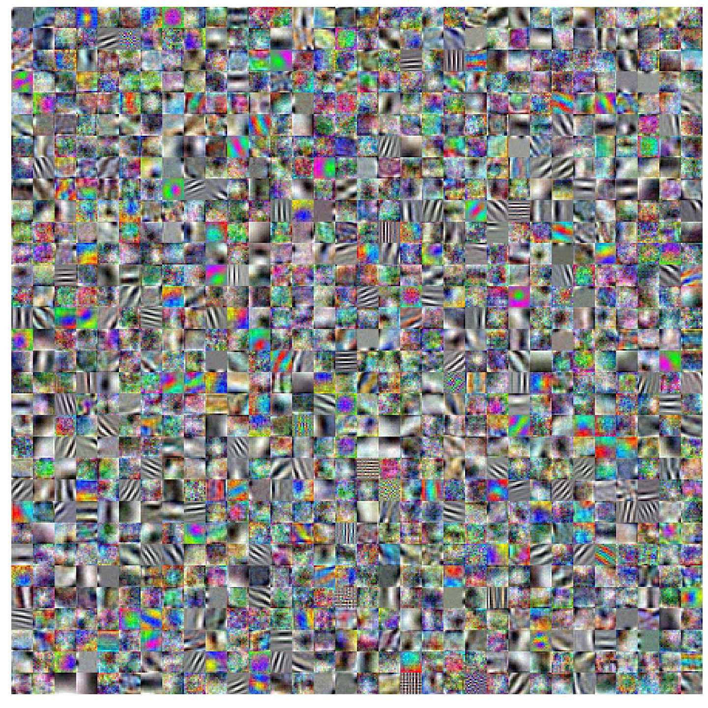
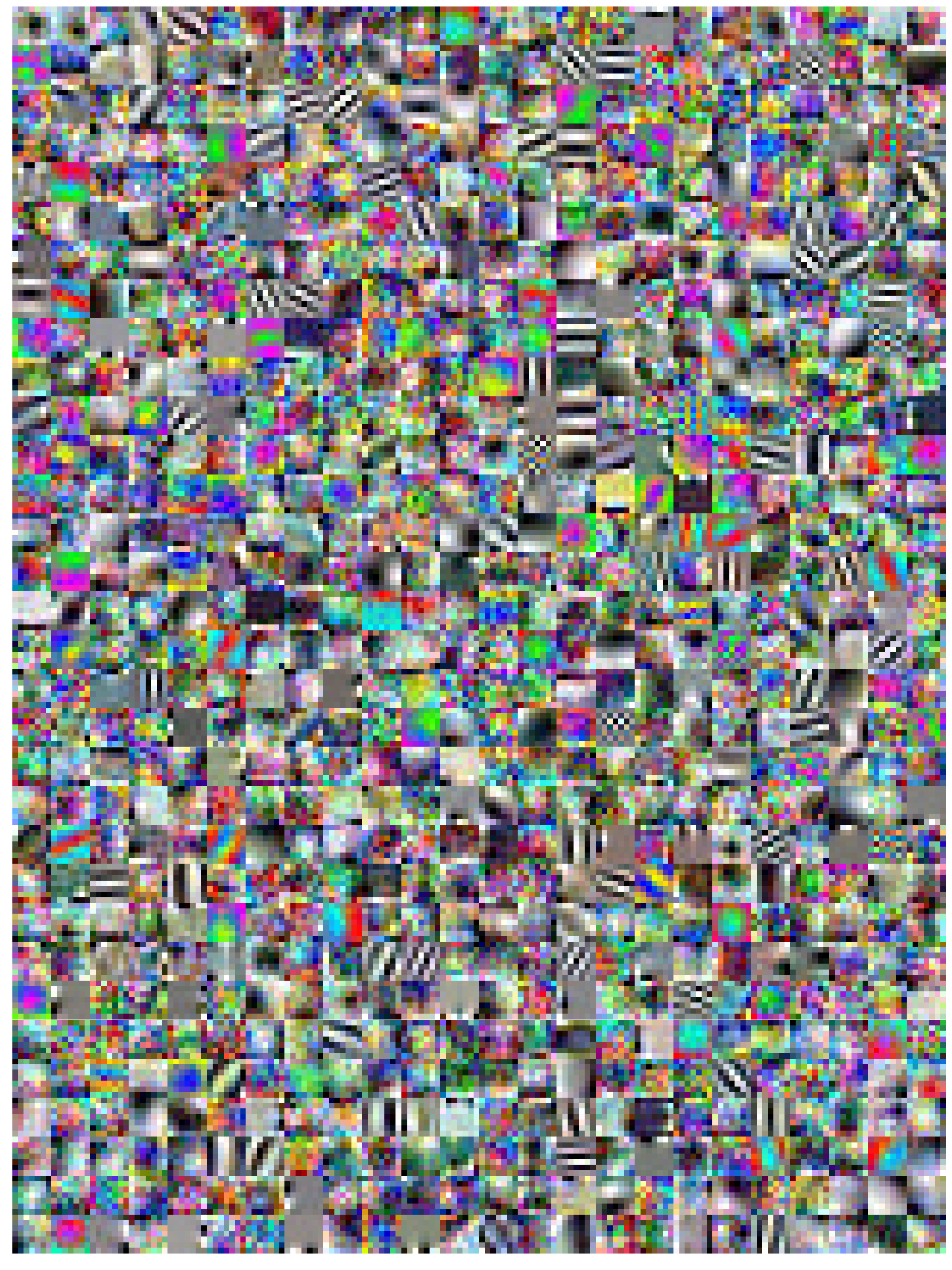
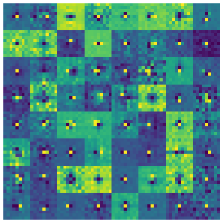
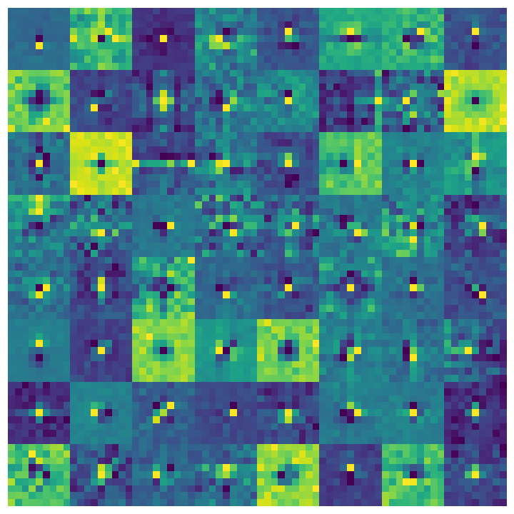
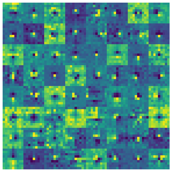
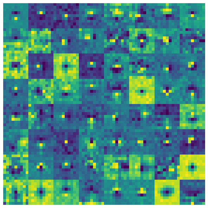
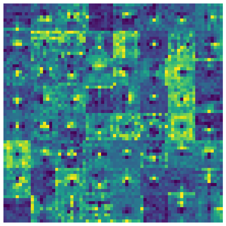
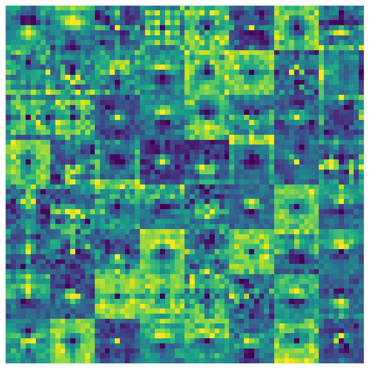
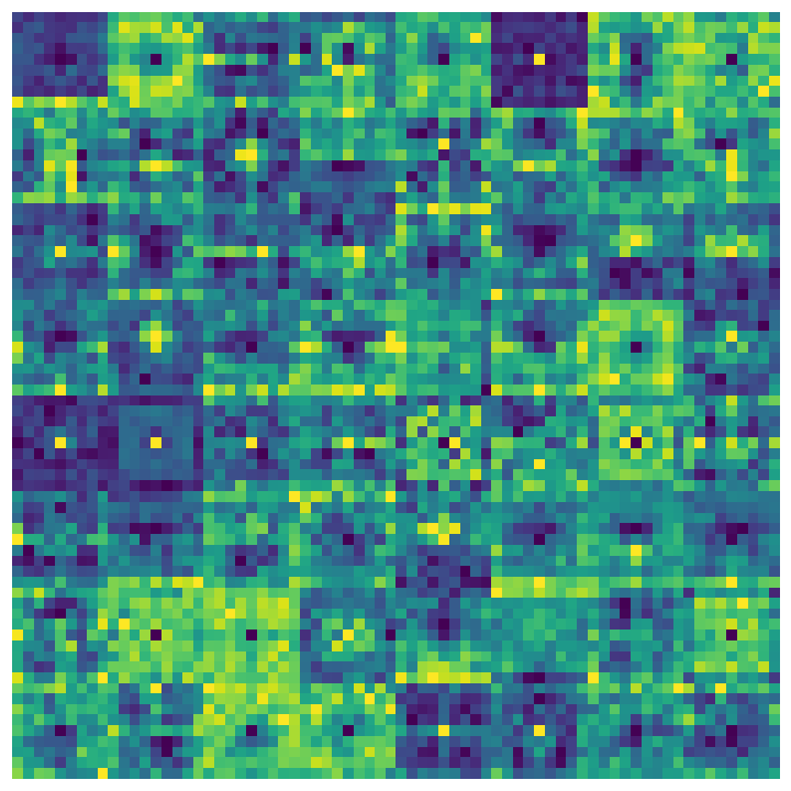
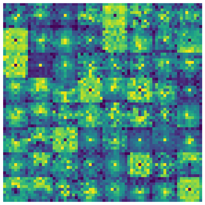
In Figure 4 and 5, we visualize the (complete) weights of the patch embedding layers of a ConvMixer-1536/20 with $p=14$ and a ConvMixer-768/32 with $p=7$, respectively. Much like Sandler et al. (2019), the layer consists of Gabor-like filters as well as “colorful globs” or rough edge detectors. The filters seem to be more structured than those learned by MLP-Mixer (Tolstikhin et al., 2021); also unlike MLP-Mixer, the weights look much the same going from $p=14$ to $p=7$: the latter simply looks like a downsampled version of the former. It is unclear, then, why we see such a drop in accuracy for larger patches. However, some of the filters essentially look like noise, maybe suggesting a need for more regularization or longer training, or even more data. Ultimately, we cannot read too much into the learned representations here.

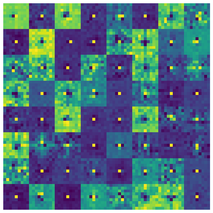
In Figure 6, we plot the hidden convolutional kernels for successive layers of a ConvMixer. Initially, the kernels seem to be relatively small, but make use of their allowed full size in later layers; there is a clear hierarchy of features as one would expect from a standard convolutional architecture. Interestingly, Touvron et al. (2021a) saw a similar effect for ResMLP, where earlier layers look like small-kernel convolution, while later layers were more diffuse, despite these layers being representated by an unconstrained matrix multiplication rather than convolution.

Appendix D Implementation

⬇

import torch.nn as nn

\parclass Residual(nn.Module):

def __init__(self, fn):

super().__init__()

self.fn = fn

\pardef forward(self, x):

return self.fn(x) + x

\pardef ConvMixer(dim, depth, kernel_size=9, patch_size=7, n_classes=1000):

return nn.Sequential(

nn.Conv2d(3, dim, kernel_size=patch_size, stride=patch_size),

nn.GELU(),

nn.BatchNorm2d(dim),

*[nn.Sequential(

Residual(nn.Sequential(

nn.Conv2d(dim, dim, kernel_size, groups=dim, padding=”same”),

nn.GELU(),

nn.BatchNorm2d(dim)

)),

nn.Conv2d(dim, dim, kernel_size=1),

nn.GELU(),

nn.BatchNorm2d(dim)

) for i in range(depth)],

nn.AdaptiveAvgPool2d((1,1)),

nn.Flatten(),

nn.Linear(dim, n_classes)

)

Figure 7: A more readable PyTorch (Paszke et al., 2019) implementation of ConvMixer, where $h$ = dim, $d$ = depth, $p$ = patch_size, $k$ = kernel_size.

⬇

def ConvMixer(h,d,k,p,n):

S,C,A=Sequential,Conv2d,lambda x:S(x,GELU(),BatchNorm2d(h))

R=type(”,(S,),{’forward’:lambda s,x:s[0](x)+x})

return S(A(C(3,h,p,p)),*[S(R(A(C(h,h,k,groups=h,padding=k//2))),A(C(h,h,1))) for i in range(d)],AdaptiveAvgPool2d(1),Flatten(),Linear(h,n))

Figure 8: An implementation of our model in less than 280 characters, in case you happen to know of any means of disseminating information that could benefit from such a length.
All you need to do to run this is from torch.nn import *.

This section presents an expanded (but still quite compact) version of the terse ConvMixer implementation that we presented in the paper. The code is given in Figure 7. We also present an even more terse implementation in Figure 8, which to the best of our knowledge is the first model that achieves the elusive dual goals of $80\%+$ ImageNet top-1 accuracy while also fitting into a tweet.

References

- Bello (2021) Irwan Bello. Lambdanetworks: Modeling long-range interactions without attention. arXiv preprint arXiv:2102.08602, 2021.
- Bello et al. (2019) Irwan Bello, Barret Zoph, Ashish Vaswani, Jonathon Shlens, and Quoc V Le. Attention augmented convolutional networks. In Proceedings of the IEEE/CVF international conference on computer vision, pp. 3286–3295, 2019.
- Chen et al. (2021) Shoufa Chen, Enze Xie, Chongjian Ge, Ding Liang, and Ping Luo. Cyclemlp: A mlp-like architecture for dense prediction. arXiv preprint arXiv:2107.10224, 2021.
- Cordonnier et al. (2019) Jean-Baptiste Cordonnier, Andreas Loukas, and Martin Jaggi. On the relationship between self-attention and convolutional layers. arXiv preprint arXiv:1911.03584, 2019.
- Cubuk et al. (2020) Ekin D Cubuk, Barret Zoph, Jonathon Shlens, and Quoc V Le. Randaugment: Practical automated data augmentation with a reduced search space. In Proceedings of the IEEE/CVF Conference on Computer Vision and Pattern Recognition Workshops, pp. 702–703, 2020.
- Dai et al. (2021) Zihang Dai, Hanxiao Liu, Quoc V Le, and Mingxing Tan. Coatnet: Marrying convolution and attention for all data sizes. arXiv preprint arXiv:2106.04803, 2021.
- d’Ascoli et al. (2021) Stéphane d’Ascoli, Hugo Touvron, Matthew Leavitt, Ari Morcos, Giulio Biroli, and Levent Sagun. Convit: Improving vision transformers with soft convolutional inductive biases. arXiv preprint arXiv:2103.10697, 2021.
- Dosovitskiy et al. (2020) Alexey Dosovitskiy, Lucas Beyer, Alexander Kolesnikov, Dirk Weissenborn, Xiaohua Zhai, Thomas Unterthiner, Mostafa Dehghani, Matthias Minderer, Georg Heigold, Sylvain Gelly, et al. An image is worth 16x16 words: Transformers for image recognition at scale. arXiv preprint arXiv:2010.11929, 2020.
- Guo et al. (2021) Jianyuan Guo, Kai Han, Han Wu, Chang Xu, Yehui Tang, Chunjing Xu, and Yunhe Wang. Cmt: Convolutional neural networks meet vision transformers. arXiv preprint arXiv:2107.06263, 2021.
- Hendrycks & Gimpel (2016) Dan Hendrycks and Kevin Gimpel. Gaussian error linear units (gelus). arXiv preprint arXiv:1606.08415, 2016.
- Hou et al. (2021) Qibin Hou, Zihang Jiang, Li Yuan, Ming-Ming Cheng, Shuicheng Yan, and Jiashi Feng. Vision permutator: A permutable mlp-like architecture for visual recognition, 2021.
- Liu et al. (2021a) Hanxiao Liu, Zihang Dai, David R So, and Quoc V Le. Pay attention to mlps. arXiv preprint arXiv:2105.08050, 2021a.
- Liu et al. (2021b) Ze Liu, Yutong Lin, Yue Cao, Han Hu, Yixuan Wei, Zheng Zhang, Stephen Lin, and Baining Guo. Swin transformer: Hierarchical vision transformer using shifted windows, 2021b.
- Loshchilov & Hutter (2018) Ilya Loshchilov and Frank Hutter. Fixing weight decay regularization in adam. 2018.
- Melas-Kyriazi (2021) Luke Melas-Kyriazi. Do you even need attention? a stack of feed-forward layers does surprisingly well on imagenet, 2021.
- Paszke et al. (2019) Adam Paszke, Sam Gross, Francisco Massa, Adam Lerer, James Bradbury, Gregory Chanan, Trevor Killeen, Zeming Lin, Natalia Gimelshein, Luca Antiga, Alban Desmaison, Andreas Kopf, Edward Yang, Zachary DeVito, Martin Raison, Alykhan Tejani, Sasank Chilamkurthy, Benoit Steiner, Lu Fang, Junjie Bai, and Soumith Chintala. Pytorch: An imperative style, high-performance deep learning library. In H. Wallach, H. Larochelle, A. Beygelzimer, F. d’ Alché-Buc, E. Fox, and R. Garnett (eds.), Advances in Neural Information Processing Systems 32, pp. 8024–8035. Curran Associates, Inc., 2019.
- Ramachandran et al. (2019) Prajit Ramachandran, Niki Parmar, Ashish Vaswani, Irwan Bello, Anselm Levskaya, and Jonathon Shlens. Stand-alone self-attention in vision models. arXiv preprint arXiv:1906.05909, 2019.
- Sandler et al. (2019) Mark Sandler, Jonathan Baccash, Andrey Zhmoginov, and Andrew Howard. Non-discriminative data or weak model? on the relative importance of data and model resolution. In Proceedings of the IEEE/CVF International Conference on Computer Vision Workshops, pp. 0–0, 2019.
- Tolstikhin et al. (2021) Ilya Tolstikhin, Neil Houlsby, Alexander Kolesnikov, Lucas Beyer, Xiaohua Zhai, Thomas Unterthiner, Jessica Yung, Daniel Keysers, Jakob Uszkoreit, Mario Lucic, et al. Mlp-mixer: An all-mlp architecture for vision. arXiv preprint arXiv:2105.01601, 2021.
- Touvron et al. (2020) Hugo Touvron, Matthieu Cord, Matthijs Douze, Francisco Massa, Alexandre Sablayrolles, and Hervé Jégou. Training data-efficient image transformers & distillation through attention. arXiv preprint arXiv:2012.12877, 2020.
- Touvron et al. (2021a) Hugo Touvron, Piotr Bojanowski, Mathilde Caron, Matthieu Cord, Alaaeldin El-Nouby, Edouard Grave, Armand Joulin, Gabriel Synnaeve, Jakob Verbeek, and Hervé Jégou. Resmlp: Feedforward networks for image classification with data-efficient training. arXiv preprint arXiv:2105.03404, 2021a.
- Touvron et al. (2021b) Hugo Touvron, Matthieu Cord, Alexandre Sablayrolles, Gabriel Synnaeve, and Hervé Jégou. Going deeper with image transformers. arXiv preprint arXiv:2103.17239, 2021b.
- Vaswani et al. (2017) Ashish Vaswani, Noam Shazeer, Niki Parmar, Jakob Uszkoreit, Llion Jones, Aidan N Gomez, Łukasz Kaiser, and Illia Polosukhin. Attention is all you need. In Advances in neural information processing systems, pp. 5998–6008, 2017.
- Wang et al. (2021) Wenhai Wang, Enze Xie, Xiang Li, Deng-Ping Fan, Kaitao Song, Ding Liang, Tong Lu, Ping Luo, and Ling Shao. Pyramid vision transformer: A versatile backbone for dense prediction without convolutions. arXiv preprint arXiv:2102.12122, 2021.
- Wightman (2019) Ross Wightman. Pytorch image models. https://github.com/rwightman/pytorch-image-models, 2019.
- Wightman et al. (2021) Ross Wightman, Hugo Touvron, and Hervé Jégou. Resnet strikes back: An improved training procedure in timm, 2021.
- Xiao et al. (2021) Tete Xiao, Mannat Singh, Eric Mintun, Trevor Darrell, Piotr Dollár, and Ross Girshick. Early convolutions help transformers see better. arXiv preprint arXiv:2106.14881, 2021.
- Yuan et al. (2021a) Kun Yuan, Shaopeng Guo, Ziwei Liu, Aojun Zhou, Fengwei Yu, and Wei Wu. Incorporating convolution designs into visual transformers. arXiv preprint arXiv:2103.11816, 2021a.
- Yuan et al. (2021b) Li Yuan, Yunpeng Chen, Tao Wang, Weihao Yu, Yujun Shi, Zihang Jiang, Francis EH Tay, Jiashi Feng, and Shuicheng Yan. Tokens-to-token vit: Training vision transformers from scratch on imagenet. arXiv preprint arXiv:2101.11986, 2021b.
- Yun et al. (2019) Sangdoo Yun, Dongyoon Han, Seong Joon Oh, Sanghyuk Chun, Junsuk Choe, and Youngjoon Yoo. Cutmix: Regularization strategy to train strong classifiers with localizable features. In Proceedings of the IEEE/CVF International Conference on Computer Vision, pp. 6023–6032, 2019.
- Zhang et al. (2017) Hongyi Zhang, Moustapha Cisse, Yann N Dauphin, and David Lopez-Paz. mixup: Beyond empirical risk minimization. arXiv preprint arXiv:1710.09412, 2017.
- Zhong et al. (2020) Zhun Zhong, Liang Zheng, Guoliang Kang, Shaozi Li, and Yi Yang. Random erasing data augmentation. In Proceedings of the AAAI Conference on Artificial Intelligence, volume 34, pp. 13001–13008, 2020.