A large catalogue of molecular clouds in the southern sky

Abstract

We present a large catalogue of molecular clouds with accurate distance estimates in the southern sky. Based on the three-dimensional (3D) dust extinction map and the best-fit extinction and distance information of over 17 million stars presented in Guo et al., we have identified 250 dust/molecular clouds in the southern sky using a hierarchical structure identification algorithm. Amongst them, 71 clouds locating at high Galactic latitudes ($b<-10$°). We have estimated the distances to the clouds by fitting the extinction versus distance profiles of the lines of sight overlapping with the clouds using a simple Gaussian dust distribution model. The typical uncertainties of the distances are less than 7 per cent. We also provide the physical properties of the individual clouds, including the linear radius, mass and surface mass density.

1 Introduction

Molecular clouds play a crucial role in the processes of star formation and galaxy evolution (Blitz & Williams, 1999). A large catalogue of molecular clouds with robust property measurements is fundamental for the studies of the physical nature and evolution of molecular clouds themselves and understanding the process of star formation and ultimately of galaxy evolution (e.g. Larson, 1981; Lombardi et al., 2010; Wang et al., 2015; Li et al., 2016; Rice et al., 2016; Lada & Dame, 2020).

Many efforts have been made to identify molecular clouds in the Milky Way and obtain their physical parameters. Most of those works are based on the radio observations of the CO emission. Based on the CO data obtained with the 5 m telescope of the Millimeter Wave Observatory, Magnani et al. (1985) identified 57 clouds at high Galactic latitudes and provided properties such as distance, size, mass, density and extinction of some of the clouds. Based on the third Galactic quadrant CO survey obtained with the 1.2 m Southern Millimeter-wave Telescope (May et al., 1993), May et al. (1997) identified 177 molecular clouds in the southern outer Galaxy and measured their distances, radii and masses. They found power-law relations between the cloud line widths and sizes, as well as between the densities and sizes. Dame et al. (2001) combined the available large-scale CO surveys into a composite survey that covers most of the sky with significant CO emission. Based on the data of Dame et al., Rice et al. (2016) and Miville-Deschênes et al. (2017) identified and measured the basic properties of molecular clouds across the Milky Way. Rice et al. (2016) identified 1,064 clouds in the Galactic plane using a dendrogram-based decomposition algorithm. Miville-Deschênes et al. (2017) recovered 8,107 molecular clouds in the entire Galactic plane by Gaussian decomposition followed by a hierarchical cluster identification method.

Dust observation serves as a complementary approach to trace the molecular gas and probe the properties of molecular clouds (Wolf, 1923; Lada et al., 1994). Based on the Digitized Sky Survey I (Lasker, 1994), Dobashi et al. (2005) produced a two-dimensional (2D) $A_{V}$ extinction map of the Galactic disk and identified 2,448 dark clouds from the map. The catalogue was later improved by Dobashi (2011), who identified 7,614 clouds across the sky based on a 2D extinction map derived from the data of the 2 Micron All Sky Survey (2MASS; Skrutskie et al., 2006). Based on the 2MASS data and the Besançon Galactic model (Robin et al., 2003), Marshall et al. (2009) mapped the three-dimensional (3D) extinction distributions toward over 1,500 dark clouds and calculated the distances and masses for 1,259 of them. Based on the 2MASS data, Lada et al. (2010), Lombardi et al. (2010) and Lombardi et al. (2011) presented near-infrared (IR) extinction maps toward nearby molecular clouds and estimated distances and masses of them. Schlafly et al. (2014) determined the distances of clouds identified by Magnani et al. (1985) and of some other well-studied nearby clouds by the method of 3D extinction mapping based on the data of PanSTARRS-1 (Chambers et al., 2016; PS1). Using similar techniques, Zucker et al. (2019, 2020) measured the distances of local molecular clouds by combining the optical and near-IR photometries with the Gaia Data Release 2 (Gaia DR2; Gaia Collaboration, 2018). Recently, Chen et al. (2020a) presented a large catalogue of 567 clouds in the Galactic plane identified from the 3D extinction maps of Chen et al. (2019) and provided their accurate distances and other physical parameters.

Most of the aforementioned studies dealt with molecular clouds in the Galactic disk of low Galactic latitudes and of regions of high Galactic latitudes in the northern sky. Only few works have analysed the molecular clouds in the southern sky, especially of regions of $b<-10\degr$ . Guo et al. (2021b) have presented 3D extinction maps of the southern sky based on the multiband photometry of the SkyMapper Southern Survey Data Release 1 (SMSS DR1; Wolf et al., 2018), Gaia DR2, 2MASS, and the Wide-Field Infrared Survey Explorer (WISE; Wright et al., 2010), and the stellar distances calculated from the Gaia DR2 parallaxes (Bailer-Jones et al., 2018). The work of Guo et al. provides us with an opportunity to fill the gap.

In the current work, we identify molecular clouds in the southern sky and calculate their accurate distances and other physical properties based on the data of Guo et al. (2021b). The structure of the paper is as following. The data and method are described in Section 2 and 3, respectively. We present our results in Section 4 and discuss them in Section 5. A summary is given in Section 6.

2 Data

The basic data adopted in the current work are from Guo et al. (2021b), including the 3D dust extinction maps of the southern sky and a catalogue containing distances and extinction values of over 17 million stars. The data can be accessed at https://registry.china-vo.org/resource/101032.

The extinction maps of Guo et al. have a sky coverage of $\sim$ 14,000 deg² within the footprint of the SMSS DR1 (Wolf et al., 2018). Guo et al. (2021b) adopted only stars that are detected in all the SkyMapper $g$, $r$ and $i$ bands with photometric uncertainties smaller than 0.08 mag in all the three bands. Their maps cover the entire southern sky (Declination $\delta<0\degr$) except for a few regions close to the Galactic plane and some isolated fields due to the missing of the SMSS DR1 data. The resolution of the maps is 6.9 arcmin at low Galactic latitudes ($|b|<10\degr$) and increases to 27.5 arcmin at $b<-30\degr$. The maps have a typical distance limit of $\sim$ 5 kpc and a distance resolution of 0.2 kpc.

The extinction values of the individual stars were estimated by the best-fit SED algorithm using the multi-band photometric data from the optical to the near-IR bands. The typical uncertainties are about 0.07 mag in $E(B-V)$ (Guo et al., 2021b). The distances of stars were adopted from the work of Bailer-Jones et al. (2018), who provide distances of 1.3 billion stars based on the Gaia DR2 parallax measurements using a simple Bayesian approach. Guo et al. (2021b) excluded stars with Gaia DR2 parallax uncertainties larger than 20 per cent, leading to a sample of over 17 million stars with robust distance and extinction values.

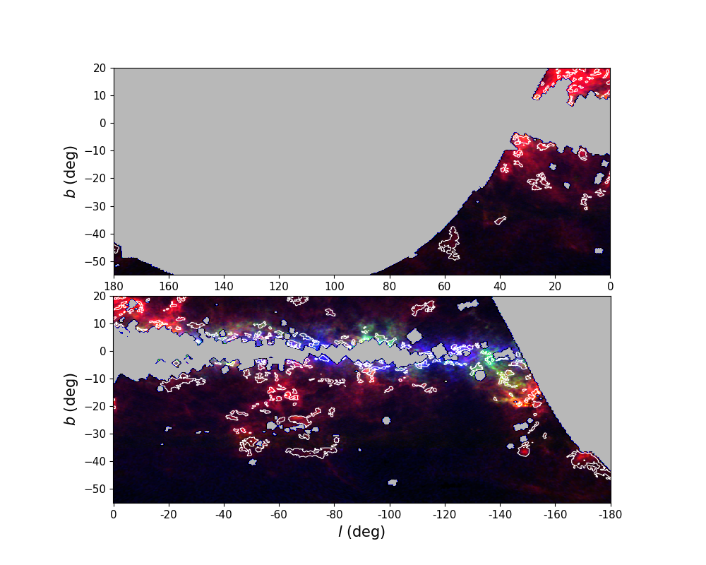
Figure 1: Spatial distributions of the molecular clouds identified in this work. The boundaries of the individual molecular clouds are marked by white polygons. The 3D dust extinction maps of Guo et al. (2021b) are represented by the background three-colour composite images, in which the red, green and blue scales correspond to the extinction values in the distance slices 0–800, 800–1600, and 1600–5000 pc from the Sun, respectively. The grey pixels, which are mostly located at the Galactic plane, are regions not covered by the extinction maps of Guo et al. (2021b).

Table 1: Catalogue of molecular clouds.

ID	$l$	$b$	$\Omega$	$r$	$d_{0}$	$\delta d$	$\delta{A_{r}}$	$M$	$\Sigma$
	($\degr$)	($\degr$)	(deg2)	(pc)	(pc)	(pc)	(mag)	($M_{\odot}$)	$(M_{\odot}$ pc-2)
1	57.63	$-$43.12	28.115	9.3	179 $\pm$ 4	70 $\pm$ 4	0.22	1494.0	5.4
2	188.65	$-$39.66	50.676	16.8	239 $\pm$ 4	126 $\pm$ 2	0.29	13024.7	14.8
3	287.4	$-$36.6	31.583	11.1	200 $\pm$ 5	69 $\pm$ 6	0.22	1583.2	4.1
4	211.1	$-$35.88	13.753	5.2	143 $\pm$ 6	41 $\pm$ 10	0.32	3401.1	39.7
5	310.87	$-$34.17	18.114	8.5	203 $\pm$ 4	53 $\pm$ 9	0.38	3112.7	13.7
6	40.29	$-$35.47	4.71	9.5	445 $\pm$ 12	171 $\pm$ 14	0.36	2024.1	7.1
7	305.59	$-$34.33	7.654	5.0	185 $\pm$ 8	45 $\pm$ 10	0.31	1259.1	15.8
8	278.87	$-$32.58	3.35	3.7	208 $\pm$ 40	47 $\pm$ 21	0.21	218.9	5.0
9	290.32	$-$30.98	3.531	3.4	184 $\pm$ 15	55 $\pm$ 14	0.29	590.7	16.2
10	9.18	$-$28.4	8.923	5.0	170 $\pm$ 6	51 $\pm$ 8	0.39	1188.2	15.1
…	…	…	…	…	…	…	…	…	…
241	260.52	$-$5.66	0.498	13.5	1943 $\pm$ 68	242 $\pm$ 85	1.05	9346.4	16.3
242	276.7	$-$3.09	0.18	9.2	2199 $\pm$ 242	389 $\pm$ 348	1.08	4595.8	17.4
243	299.81	5.01	0.996	24.5	2490 $\pm$ 295	940 $\pm$ 2301	1.7	27417.5	14.6
244	237.23	$-$4.16	0.977	24.1	2476 $\pm$ 239	825 $\pm$ 734	1.29	23392.3	12.8
245	296.01	$-$3.98	1.776	36.4	2776 $\pm$ 177	605 $\pm$ 393	0.69	53535.6	12.8
246	276.12	$-$2.57	0.14	9.2	2492 $\pm$ 264	452 $\pm$ 366	1.33	4218.3	15.9
247	282.97	1.62	0.9	27.2	2913 $\pm$ 307	775 $\pm$ 417	1.6	44903.1	19.3
248	235.37	$-$4.58	0.718	21.1	2529 $\pm$ 191	492 $\pm$ 356	1.0	17269.9	12.4
249	286.92	3.34	1.577	35.1	2839 $\pm$ 232	525 $\pm$ 2944	0.6	32475.8	8.4
250	254.12	1.69	4.937	77.0	3520 $\pm$ 133	628 $\pm$ 269	0.6	187425.6	10.1

Note. The Table is available in its entirety in the online version of this paper and also from the link http://paperdata.china-vo.org/guo/cloud/cloud_para.fits

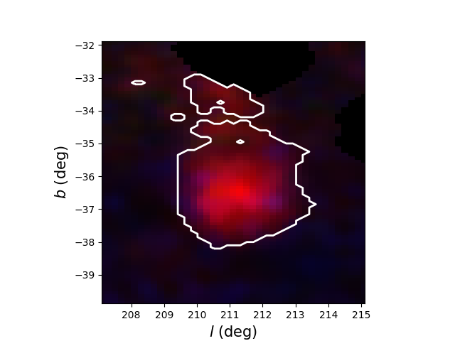
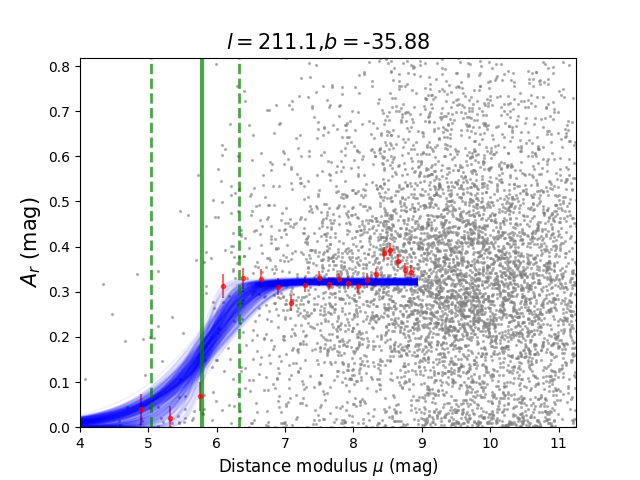
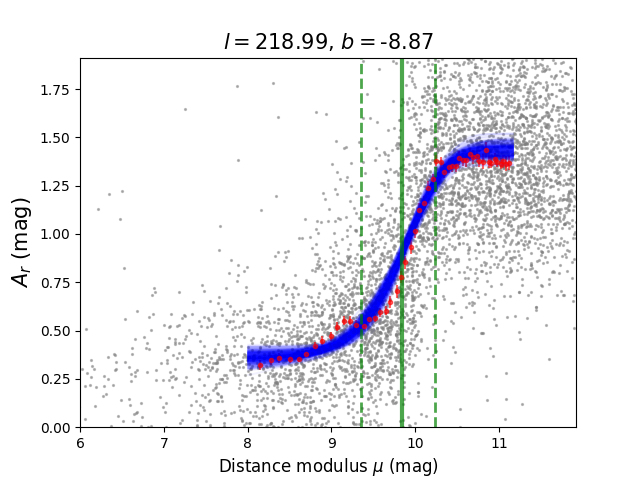
Figure 2: Distance determinations for two example molecular clouds: Cloud No. 4 (upper panel) and No. 180 (Mon R2; bottom panel). In the left panel, we show the sky coverage of the clouds by the white polygons. The 3D dust extinction maps of Guo et al. (2021b) are illustrated by the background three-colour composite images, in which the red, green and blue scales correspond to the extinction values of $A_{r}$ in the distance slices 0–800, 800–1600, and 1600–5000 pc from the Sun, respectively. In the right panel, we show the $r$-band extinction profiles of the sightlines overlapping with the example clouds. The red circles and errorbars are respectively the median values and standard errors in the individual distance bins of bin-size 50 pc. Blue curves are the best-fit extinction profiles $A_{r}(d)$ of the 300 randomly generated star samples. Vertical solid and dashed lines mark the resultant distance $d_{0}$ and width $\delta d$ of the clouds, respectively.

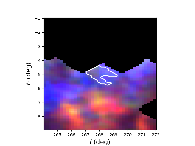
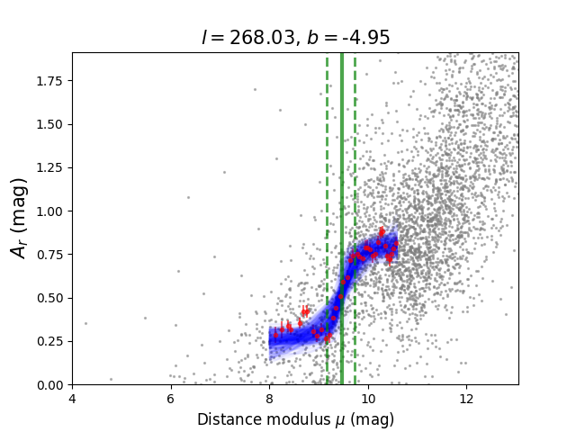
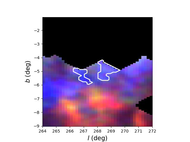
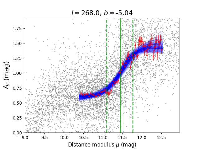
Figure 3: Same as Fig. 2 but for Clouds No. 182 (upper panel) and 237 (bottom panel), that are only partly covered by the data of Guo et al. (2021b).

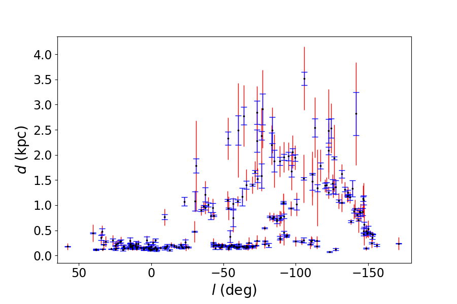
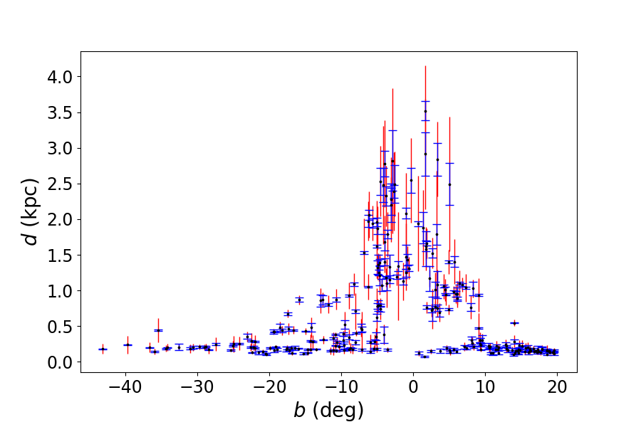
Figure 4: Distances of clouds identified in this work plotted against their Galactic longitudes (left panel) and Galactic latitudes (right panel). The blue and red error bars represent the distance uncertainties and the derived widths/depths ($\delta d$) of the clouds, respectively.

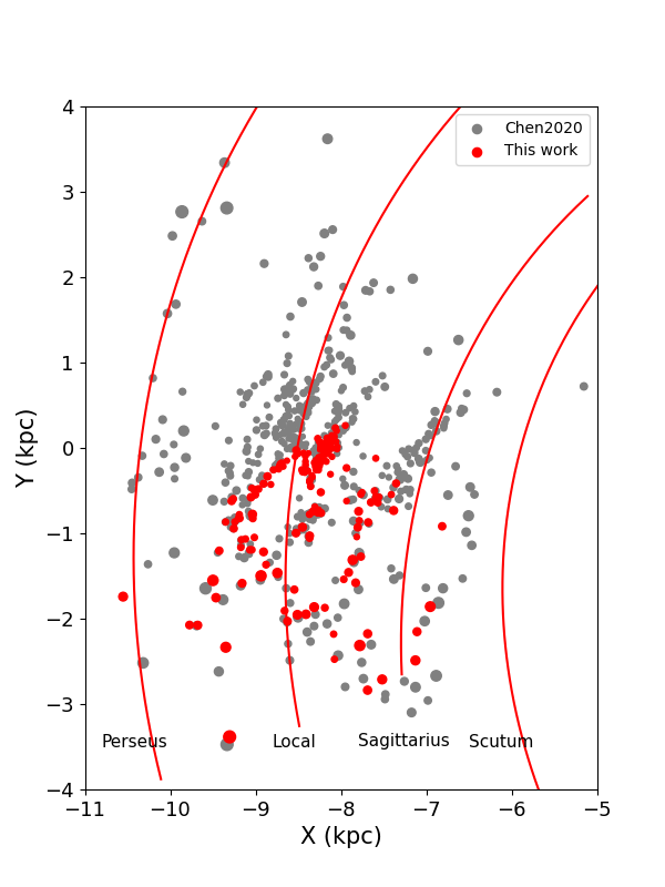
Figure 5: Spatial distribution of the molecular clouds identified in the current work (red dots) and Chen et al. (2020a; grey) in the Galactic coordinates. The sizes of the dots indicate the radius of the clouds. The Sun, with the coordinate of ($X,Y$) = ($-$8.34, 0) kpc, is located at the centre of the plot. The solid red lines are the best-fitting spiral arm models of the Scutum, Sagittarius, Local, and Perseus Arms from Chen et al. (2019).

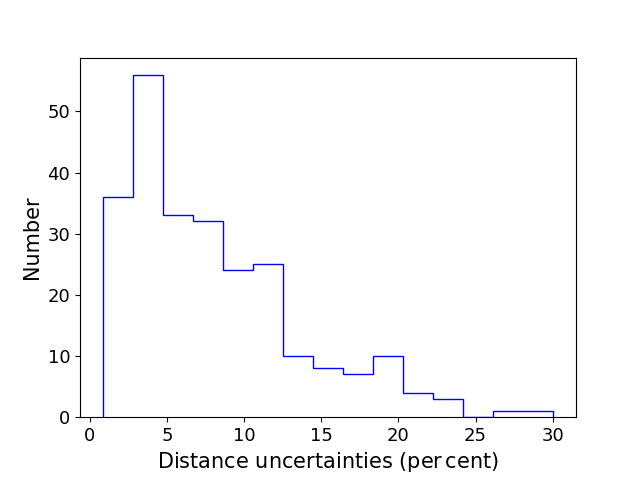
Figure 6: Distribution of the distance uncertainties of our catalogued molecular clouds.

3 Method

In the current work, we have adopted a method similar as in the work of Chen et al. (2020a). The method comprises three steps: the first step is to isolate the individual molecular clouds from the 3D extinction maps; the second step to estimate the distances of the identified molecular clouds; and the third step to calculate their physical properties.

3.1 Molecular cloud identification

To identify the molecular clouds, we firs interpolate the extinction maps of Guo et al. to a 3D data cube of differential extinction values contributed by the local dust grains, $\Delta A_{r}$ (in units of mag kpc^-1), of which the three dimensions correspond to the Galactic coordinates $l$ and $b$, and the distance $d$. We adopt resolutions of 0.2°,  0.1° and 0.2 kpc in $l$, $b$ and $d$, respectively. The nearest neighbour inter- polation is adopted in the current work. The python program dendrogram (Rosolowsky et al., 2008) is applied to the 3D data cube to identify the molecular clouds. Dendrograms are topological representations of the hierarchical structure of nested isosurfaces in $N$-dimensional intensity data. The dendrogram algorithm has three input parameters: (i) “min_value”, a minimum absolute intensity threshold required to mask any structures that peak below it; (ii) “min_delta”, a minimum intensity contrast required to exclude any local maxima identified because of the noise; and (iii) “min_npix”, a minimum number of pixels (volume elements in the $lbd$ space) that a structure should contain. We have tried different sets of input parameters. We have tried different sets of input parameters and visually check the resulting clumps. Eventually, we set min_value = 0.06 mag kpc^-1, min_delta = 0.08 mag kpc^-1 and min_npix = 20. Independent structure ‘leaves’ produced by the dendrogram algorithm represent regions of density enhancements and are identified as isolated molecular clouds in the current work. We note that in the current work, we have applied the dendrogram algorithm in the $l,b$ and $d$ space. As the pixel volumes increase with the distances, our algorithm would be less sensitive to the small distant clouds.

3.2 Distance measurement

Since the distance resolution of the adopted extinction map is only 0.2 kpc, the cloud distances yielded by the dendrogram algorithm have relatively large errors. In the current work, we estimate the cloud distances from the extinction profiles of the sightlines toward the individual clouds (e.g. Schlafly et al., 2014; Chen et al., 2017; Yu et al., 2019; Chen et al., 2020a; Chen et al., 2020b; Guo et al., 2021a). The distance to a cloud can be estimated by locating the position where there is a sharp increase (‘jump’) of extinction in the extinction profile, caused by the high dust density of the molecular cloud.

The $lbd$ 3D spatial ranges of the individual clouds are provided by the dendrogram algorithm. We select all stars in the catalogue of Guo et al. (2021b) that fall within the $l$ and $b$ ranges of a given cloud. We then fit the extinction and distance relation $A_{r}(d$) of the sightline toward the cloud, established by the distances and extinction values of the selected stars, to estimate the distance of the cloud. In the current work, we assume that the increase of the extinction within the distance range of the cloud is all caused by the dust grains in the cloud (Chen et al., 2020a; Guo et al., 2021a). The extinction profile within the distance range of the cloud is then fitted by,

$$A_{r}(d)=A_{r}^{0}+A_{r}^{1}(d)\quad$if$\quad d_{\rm min}<d<d_{\rm max},$$ (1)

where $A_{r}^{0}$ is the foreground extinction, $A_{r}^{1}(d)$ is the extinction contributed by the dust in the cloud at distance $d$, and $d_{\rm min}$ and $d_{\rm max}$ are respectively the lower and upper limits of the distance range of the cloud provided by the dendrogram algorithm. Assuming a simple Gaussian distribution of dust in the cloud (Chen et al., 2017; Zhao et al., 2020; Guo et al., 2021a), we have,

$$A_{r}^{1}(d)=\frac{\delta A_{r}}{2}[1+{\rm{erf}}(\frac{d-d_{0}}{\sqrt{2}\delta d})],$$ (2)

where $\delta A_{r}$ is the total $r$-band extinction contributed by the dust in the cloud, $d_{\rm 0}$ the distance of the cloud and $\delta d$ the width of the extinction jump.

For each cloud, the foreground extinction $A_{r}^{0}$, distance of the cloud $d_{\rm 0}$, the ‘jump’ width $\delta d$ and amplitude $\delta A_{r}$ are free parameters to fit. As there could be more than one cloud along a given line of sight, only the extinction profile within the distance range $d_{\rm min}-$ 0.2 kpc $<d<d_{\rm max}$ + 0.2 kpc is fitted to avoid the contamination of other clouds. We employ a sliding window of width 25 pc with a step of 50 pc to obtain median values of extinction for the individual distance bins. The binned median extinction values are then fitted using the extinction model described above with the python Markov Chain Monte Carlo (MCMC) algorithm emcee (Foreman-Mackey et al., 2013). We adopt the likelihood

$$\mathcal{L}=\prod_{n=1}^{N}\frac{1}{\sqrt{2\pi}\sigma_{n}}{\rm{exp}}(\frac{-({A_{\rm{r}}}^{n}-{A_{\rm{r}}}^{n}(d))^{2}}{2{\sigma_{n}}^{2}}),$$ (3)

where ${A_{\rm{r}}}^{n}$ and ${A_{\rm{r}}}^{n}(d)$ are the $n$th binned median $r$-band extinction values derived from the individual stars and that modeled by Equation (1), respectively, and $\sigma_{n}$ is the standard error of the $n$th binned median extinction. We adopt the priors

$$P(A_{r}^{0},d_{\rm 0},\delta A_{r},\delta d)=\begin{cases}1\quad\text{if}\,\,\begin{cases}0.0\leq A_{r}^{0}<A_{r,\rm{max}},\\ d_{\rm min}-0.2\,{\rm kpc}<d_{\rm 0}<d_{\rm{max}}+0.2\,{\rm kpc},\\ 0.0<\delta A_{r}<A_{r,\rm{max}},\\ 0.0<\delta d<d_{\rm max}-d_{\rm min},\\ \end{cases}\\ 0\quad\text{else}.\end{cases}$$

$A_{r,\rm{max}}$ is the maximum extinction value of all the selected stars.

The Monte Carlo method (Wall & Jenkins, 2003) is adopted to estimate the uncertainties of the resultant parameters. For each cloud, we randomly generate 300 samples of stars sampling the distance and extinction errors. The fit algorithm is applied to all the samples and the rms scatters of the best-fit parameters are adopted as their errors.

We have also adopted other bin sizes, such as 30 pc, 50 pc and 70 pc, for the fitting of the extinction profiles, which yield very similar results. We note that in the current work, we treat the molecular cloud as a whole and fit the median extinction and distance profile of the cloud, instead of extinction profiles of the individual stars (Schlafly et al., 2014; Zucker et al., 2019; Chen et al., 2020a). For comparison, we have selected four example clouds and estimated their parameters using both our method and the method from Chen et al. (2020a). Results from the two approaches are almost identical.

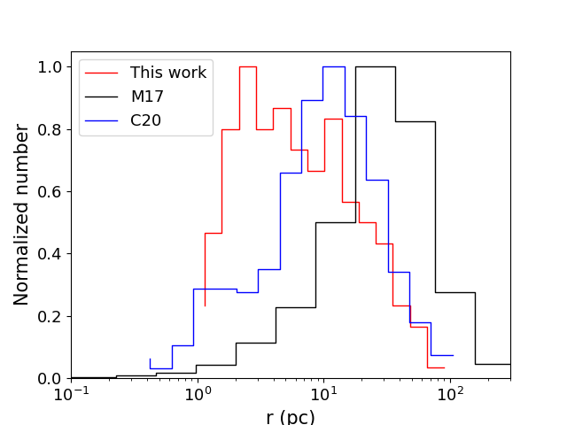
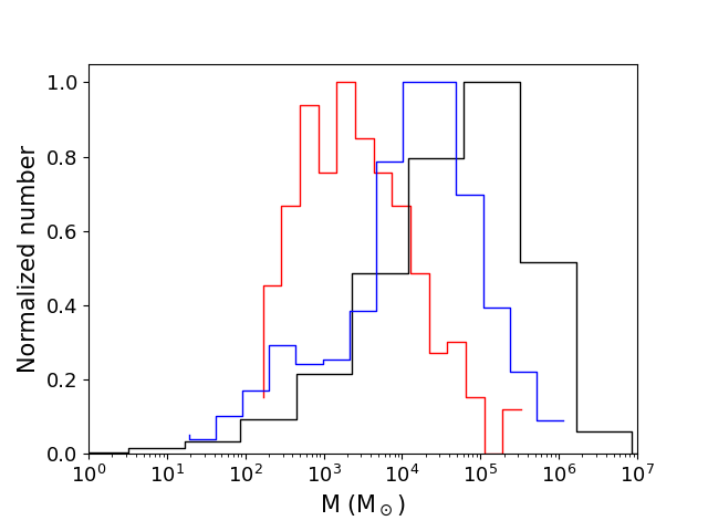
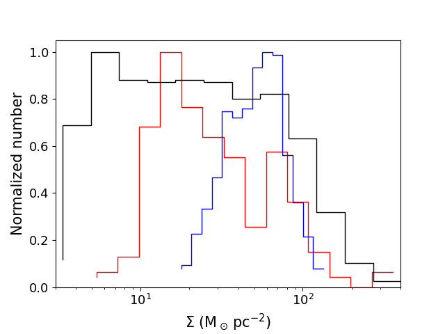
Figure 7: Normalized histograms distributions of the physical properties, including radii (upper panel), masses (middle panel), and surface mass densities (bottom panel), of our catalogued molecular clouds (red), and of those from Miville-Deschênes et al. (2017; black) and from Chen et al. (2020a; blue).

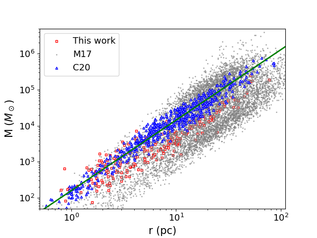
Figure 8: Radius-mass relation for clouds cataloged in this work (red squares) and for those from Miville-Deschênes et al. (2017; gray dots), and from Chen et al. (2020a; blue triangles). The green line is the best-fit radius-mass relation for clouds presented in the current work and in Chen et al. (2020a).

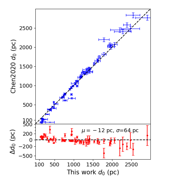
Figure 9: Comparison of our cloud distances with those from Chen et al. (2020a). A dashed line denoting complete equality is over-plotted to guide the eyes.

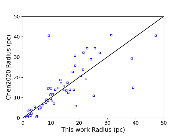
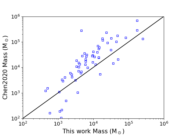
Figure 10: Comparison of physical parameters, including radius (upper panel) and mass (bottom panel) obtained in the current work with those of Chen et al. (2020a). A black lines denoting complete equality is over- plotted to guide the eyes in each panel.

3.3 Physical parameters

With the distances derived, we are then able to compute the properties of the identified molecular clouds, following Chen et al. (2020a).

(i) Solid angle $\Omega$, in units of deg²,

$$\Omega=\sum_{i=0}^{N}\Delta l\Delta b\,{\rm cos}b_{i},$$ (4)

where $\Delta l=$ 0.2° and $\Delta b=$ 0.1° are respectively the $l$ and $b$ angular resolution of our 3D data cube, $i$ is the pixel index and $b_{i}$ the Galactic latitude of the $i$th pixel.

(ii) Area S, in units of pc²,

$$S=\Omega\,d_{0}^{2}.$$ (5)

(iii) Linear radius $r$, in units of pc,

$$r=\sqrt{\frac{S}{\pi}}.$$ (6)

(iv) Mass $M$, in units of $M_{\odot}$,

$$M=\frac{\mu m_{{}_{\rm H}}A_{V}S}{DGR}.$$ (7)

(v) Surface density $\Sigma$, in units of $M_{\odot}$ pc²,

$$\Sigma=\frac{M}{S}.$$ (8)

In the current work, we adopt $\mu$ = 1.37 (Lombardi et al., 2011) is the mean molecular weight, $m_{{}_{\rm H}}$ the mass of hydrogen atom, $A_{V}$ the optical extinction of the cloud converted from $A_{r}$ using the extinction law of Yuan et al. (2013), $A_{V}$ = 1.15$A_{r}$, and $DGR$ = 4.15$\times$ 10^-22 mag cm² (Chen et al., 2015) the dust-to-gas ratio. Chen et al. (2015) have combined the extinction map with the Hi and CO observations to study the correlation between the dust extinction and interstellar gas content at inter-mediate and high Galactic latitudes. The average value of $DGR$ deduced by Chen et al. (2015), 4.15$\times$ 10^-22 mag cm², is slightly smaller than the most cited value derived by Bohlin et al. (1978), 5.3$\times$ 10^-22 mag cm². Literature values of $DGR$ vary by a factor of 2, from $\sim$ 3.5 to 7.0$\times$ 10^-22 mag cm² (Shull & van Steenberg, 1985; Diplas & Savage, 1994; Liszt, 2014; Zhu et al., 2017). In addition, Chen et al. (2015) found a factor of $\sim$ 2 cloud-to-cloud variations in the $DGR$ values amongst the individual molecular clouds.

4 Result

In the current work, we have identified 250 molecular clouds in the southern sky from the Guo et al. 3D extinction maps. Distances as well as other physical properties, such as the radius, mass and surface density, of the individual clouds are derived. The spatial distribution map of these clouds is presented as Fig. 1. A large fraction of the identified isolated clouds locate near the Galactic plane. However, due to the missing data of SMSS DR1 in a few regions close to the Galactic plane, we note that for some clouds, only parts of them are identified by our algorithm. Radii, masses and surface densities of those clouds may be biased due to the incompleteness of data. However, their distances estimates should not be affected. 71 out of the 250 identified clouds locate at high Galactic latitudes ($b<-10\degr$). Most of these clouds are fully covered in our work. The full result is listed in Table 1. Each row of Table 1 contains the information of an identified molecular cloud: position $l$ and $b$, solid angle $\Omega$, radius $r$, distance $d_{0}$, width of the extinction jump $\delta d$, total extinction $\delta A_{r}$, mass $M$ and surface density $\Sigma$.

4.1 Distances of the molecular clouds

Our algorithm of distance determination was successfully applied to all the identified 250 clouds. Typically, we are able to select $\sim$ 2,500 stars in the lines of sight overlapping with a given molecular cloud from the catalogue of Guo et al. (2021b). For all the clouds, significant extinction jumps produced by dust in the corresponding molecular clouds are clearly visible in the distance ranges deduced by the dendrogram algorithm and they are nicely fitted by our extinction model. We show the distance fitting results of four example molecular clouds in Fig. 2 and Fig. 3. Analogous figures for all the catalogued molecular clouds are available online.

In the upper row of Fig. 2, we show the distance determination of a newly identified molecular cloud that locates at high Galactic latitudes in the southern sky (Cloud No. 4; $b\sim-36$ °). The distance, $d=$ 143 $\pm$ 7 pc, shows it is very close to the Sun, as expected. The number of stars that are foreground to the cloud is relatively small due to the saturation effects of the photometric data. But as shown in the Figure, we have enough foreground stars to identify the position of the extinction jump with a relatively small uncertainty. The width of the extinction jump is only $\delta d=$ 41 pc. It is mainly contributed by the intrinsic depth of the cloud, as the distance uncertainties of those nearby stars given by Gaia DR2 are small. In the bottom row of Fig. 2, we show the distance determination of the molecular cloud Mon R2 (No. 180) located at $b\sim-$9°. The resultant distance of the cloud is $d_{0}=$ 928 $\pm$ 16 pc. The width of the extinction jump is $\delta d$ = 184 pc, larger than that of the closer cloud No. 4. This is mainly due to the larger distance uncertainties for more distant stars from the Sun.

In Fig. 3, we show the results of our extinction profile fitting procedure for two molecular clouds located close to the Galactic plane: Clouds No. 182 and 237, both at $b\sim-$5°. Both clouds are not fully covered by the 3D extinction maps of Guo et al. We are only able to identify parts of them. Along a given line of sight close to the Galactic plane, there are usually more than one molecular clouds that locate at different distances. This leads to more than one extinction jump in the extinction profile. For the two example clouds shown in Fig. 3, two significant extinction jumps are visible in each profile. Thanks to the distance limits provided by the dendrogram algorithm, we are able to isolate the true extinction jumps of the catalogued clouds and estimate their accurate distances. The resultant distances of Cloud No. 182 and 237 are, respectively, $d_{0}=$ 781$\pm$ 43 pc and 1,957 $\pm$ 61 pc, and the widths of the extinction jumps are $\delta d=$ 103 and 302 pc, respectively.

We plot the centre longitudes $l$ and latitudes $b$ of all the catalogued molecular clouds against distances $d_{0}$ in Fig. 4. The distances to our identified clouds range between $d_{0}\approx$ 70 pc and 3,500 pc. The distribution of our catalogued clouds shows clearly the large-scale structure of the Galactic disk (the Galactic spiral structure; see also Sect. 5.2 of Chen et al. 2020a). High Galactic latitude ($|b|>$10°) molecular clouds are mostly local ($d_{0}<$ 200 pc). For regions of Galactic longitudes 0°$<l<$50° , due to the lack of data at low Galactic latitudes ($|b|<$10°), our identified molecular clouds are all local. The widths of the extinction jumps $\delta$d increase with the distances of the clouds. They are the results of the combination of the intrinsic depths of the clouds and the distance uncertainties of the individual stars. Assuming that the molecular clouds are spherical, the depths of the clouds are usually less than 100 pc. Thus for distant clouds, the widths of the extinction jumps $\delta$d are mainly dominated by the distance uncertainties of the individual stars.

Fig. 5 plots the spatial distribution of our catalogued molecular clouds in the $X-Y$ plane. All our sample molecular clouds are located in the third and fourth Galactic quadrants. The distribution of molecular clouds from Chen et al. (2020a) is also overplotted in the Figure for comparison. Chen et al. (2020a) have isolated 567 molecular clouds from the 3D extinction maps of Chen et al. (2019) and derived their distances and physical properties. The molecular clouds in the southern sky identified in the current work have a very similar spatial distribution with those from Chen et al. (2020a). They may be spatially associated with the spiral arms and the arm branches or spurs of the Milky Way.

Owing to the high precision of the Gaia DR2 parallax measurements for stars within 3.5 kpc from the Sun and the large number of stars that trace the extinction profiles of sightlines toward the individual clouds, we are able to obtain distances of the catalogued clouds with high precision. In Fig. 6, we show a histogram distribution of the resultant distance uncertainties of the individual clouds. The median distance uncertainty of the catalogued clouds is $\sim$ 7 per cent. About 70 per cent of the catalogued clouds have distance errors smaller than 10 per cent. A few clouds have large relative distance uncertainties ($>$20 per cent). They are mainly local molecular clouds with very small distances. For these clouds, the quality of extinction profile fits is relatively poor due to the relatively small number of foreground stars.

4.2 Physical properties of the molecular clouds

The derived physical properties, including radius $r$, mass $M$, and surface density $\Sigma$, of the individual clouds are also listed in Table 1. For the catalogued clouds, their radii range from $\sim$ 1 to 77 pc, with a median value of 5 pc; their masses range from $\sim$ 7.5$\times 10^{1}$ to 2.5$\times 10^{5}$ M_⊙, with a median value of 1.7$\times 10^{3}$ M_⊙; and their surface densities from $\sim$ 3 to 310 M_⊙ pc^-2, with a median value 20 M_⊙ pc^-2. The distributions of the radii, masses and surface densities of the molecular clouds are presented in Fig. 7. For comparison, we also show the distributions of the corresponding properties of clouds from Miville-Deschênes et al. (2017) and Chen et al. (2020a). Miville-Deschênes et al. (2017) identified 8,107 molecular clouds and assigned their properties based on the CO data of Dame et al. (2001). Chen et al. (2020a) isolated 567 molecular clouds in the Galactic disk and derived their properties based on the 3D extinction maps and stellar catalogue of Chen et al. (2019). Our catalogued clouds have property ranges similar to those of the previous studies. However, our catalogued clouds have smaller peak radius and mass than those from Miville-Deschênes et al. (2017) and Chen et al. (2020a). This is largely due to the incomplete sky coverage of the molecular clouds close to the Galactic plane.

In Fig. 8, we plot the masses of our catalogued clouds against their radii. The mass-size relations derived from Miville-Deschênes et al. (2017) and Chen et al. (2020a) are also over-plotted in the Figure for comparison. The mass-size relation of our catalogued molecular clouds of radii smaller than $\sim$ 10 pc or masses smaller than $\sim$ 5$\times 10^{3}$ M_⊙ is consistent with those from the previous studies. While for the molecular clouds of large masses/radii in our catalogue, the mass-size relation is biased to smaller masses compared to the literature. Since most of those large mass clouds are located close to the Galactic plane, they are not fully covered by the extinction maps of Guo et al. (2021b) due to the lack of good-quality SMSS DR1 data (Wolf et al., 2018). The missing parts of the clouds are usually those closer to the Galactic plane, where the extinction is high. This indicates that we are only able to isolate the low density parts of those Galactic plane clouds, leading to a bias in the resultant mass-size relation.

5 Discussion

Table 2: Comparison of our cloud distances with the literature values.

Name	ID	$l$	$b$	$d_{0}$	Literature $d_{0}$
		($\degr$)	($\degr$)	(pc)	(pc)
Ophiuchus	115	358.09	15.54	139 $\pm$ 10	139a, 125b, 142c, 141d
Ophiuchus	116	350.12	16.83	148 $\pm$ 4	139a, 125b, 142c, 141d
Ophiuchus	120	355.81	15.98	134 $\pm$ 27	139a, 125b, 142c, 141d
Ophiuchus	125	356.22	17.15	134 $\pm$ 18	139a, 125b, 142c, 141d
Orion	141	206.65	$-$19.33	418 $\pm$ 3	484b, 389e, 414f, 371g
Orion	142	212.92	$-$19.38	423 $\pm$ 27	484b, 389e, 414f, 371g
Orion	143	208.42	$-$16.59	444 $\pm$ 8	484b, 389e, 414f, 371g
Orion	144	207.06	$-$14.98	429 $\pm$ 5	484b, 389e, 414f, 371g
Orion	173	212.93	$-$18.56	486 $\pm$ 48	484b, 389e, 414f, 371g
Orion	174	210.48	$-$18.22	438 $\pm$ 28	484b, 389e, 414f, 371g
Orion	175	210.06	$-$17.37	459 $\pm$ 30	484b, 389e, 414f, 371g
Orion	176	211.19	$-$14.17	483 $\pm$ 58	484b, 389e, 414f, 371g
Chamaeleon	26	304.53	$-$21.94	193 $\pm$ 12	192h, 184i, 188i
Chamaeleon	32	294.25	$-$19.32	163 $\pm$ 30	192h, 184i, 188i
Chamaeleon	33	304.42	$-$19.07	209 $\pm$ 9	192h, 184i, 188i
Chamaeleon	34	299.98	$-$17.24	161 $\pm$ 11	192h, 184i, 188i
Chamaeleon	35	302.45	$-$17.56	197 $\pm$ 19	192h, 184i, 188i
Chamaeleon	38	294.29	$-$16.9	195 $\pm$ 8	192h, 184i, 188i
Chamaeleon	39	296.8	$-$15.98	186 $\pm$ 4	192h, 184i, 188i
Chamaeleon	40	302.94	$-$16.4	192 $\pm$ 27	192h, 184i, 188i
Chamaeleon	44	302.82	$-$14.27	175 $\pm$ 5	192h, 184i, 188i
Chamaeleon	45	294.24	$-$14.7	175 $\pm$ 9	192h, 184i, 188i
Chamaeleon	48	298.9	$-$13.47	177 $\pm$ 6	192h, 184i, 188i
Lupus	104	353.62	14.22	153 $\pm$ 9	165j, 140k, 155l, 160m, 175n
Lupus	107	349.41	14.66	173 $\pm$ 18	165j, 140k, 155l, 160m, 175n
Lupus	110	350.77	14.5	149 $\pm$ 31	165j, 140k, 155l, 160m, 175n
Lupus	116	350.12	16.83	148 $\pm$ 4	1165j, 140k, 155l, 160m, 175n
Lupus	120	355.81	15.98	134 $\pm$ 27	165j, 140k, 155l, 160m, 175n
Mon R2	180	218.99	$-$8.87	928 $\pm$ 15	952b, 905g, 830o, 867p
Mon R2	194	219.58	$-$10.73	875 $\pm$ 30	952b, 905g, 830o, 867p

Note. References: ^a Mamajek (2008), ^bSchlafly et al. (2014), ^cOrtiz-León et al. (2017), ^dOrtiz-León et al. (2018), ^eMenten et al. (2007), ^fSandstrom et al. (2007), ^gLombardi et al. (2011), ^hRoccatagliata et al. (2018), ⁱVoirin et al. (2018), ^jFranco (1990), ^kHughes et al. (1993), ^lLombardi et al. (2008), ^mDzib et al. (2018), ⁿGalli et al. (2020) ^oHerbst & Racine (1976), ^pChen et al. (2020a).

5.1 Comparison with Chen et al. (2020a)

Here we compare our derived distances and physical properties of the molecular clouds with those obtained by Chen et al. (2020a). There are 65 molecular clouds that are in common to the two studies. In Fig. 9, we compare our derived distances with those of Chen et al. (2020a). The agreement is very good. The mean and scatter of the differences are only $-$12 pc and 64 pc, respectively.

In Fig. 10 we compare our resultant radii and masses of clouds with those of Chen et al. (2020a). Our radius and mass estimates, correlate well with those of Chen et al. but are systematically lower. This is again largely due to the incomplete sky coverage of the molecular clouds in the current work.

5.2 Distances to some well studied giant molecular clouds

We have selected 5 famous and well studied giant molecular clouds from our catalogue. The distance estimates of those 5 clouds in the literature are collected and compared to our values for verify our results. The comparison is presented in Table 2. Overall, our results are well consistent with the values in the literature.

The Ophiuchus molecular cloud complex is one of the most nearby giant molecular clouds. In this work, we have isolated 4 clouds that should belong to the complex, which has a distances ranging from 134 and 148 pc. In the earlier studies, the distance of the Ophiuchus cloud was estimated to be $d_{0}=$ 139 $\pm$ 6 pc (Mamajek, 2008), 125 pc (Schlafly et al., 2014), 142 pc (Ortiz-León et al., 2017) and 141 pc Ortiz-León et al. (2018), which are all in good agreement with our results.

The Orion molecular cloud complex is one of the most extensively studied molecular clouds in our Milky Way, covering a large sky area. We have identified 8 isolated clouds belonging to this complex. They have distances between $\sim$ 420 and 480 pc, in good agreement with the estimates of Menten et al. (2007; 389 $\pm$ 23 pc), Sandstrom et al. (2007; 414 $\pm$ 7 pc) and Schlafly et al. (2014; $\sim$ 360 to 630 pc), but slightly larger than the result of Lombardi et al. (2011; 371 $\pm$ 10 pc).

Chamaeleon is a well studied giant cloud south of the Galactic plane ($l\sim$ 300°, $b\sim-$15°). We have identified 11 clouds probably belonging to it in the current work. They have distances around $\sim$ 182 pc, in very good agreement with the results in the literature: 182 pc (Roccatagliata et al., 2018) and 188 and 184 pc (Voirin et al., 2018).

The Lupus molecular cloud complex is one of the largest low-mass star-forming regions (Comerón, 2008). Previous distances estimate of the Lupus complex are 165 $\pm$ 15 pc (Franco, 1990), 140 $\pm$ 20 pc (Hughes et al., 1993), 155 $\pm$ 8 pc (Lombardi et al., 2008), $\sim$ 160 pc (Dzib et al., 2018) and 175 $\pm$ 1 pc (Galli et al., 2020). Those values compare very well with our determination ($\sim$ 135 to 175 pc).

The Monoceros R2 region (Mon R2) is a chain of reflection nebulae extending over 2° in the constellation Monoceros (van den Bergh, 1966; Lombardi et al., 2011). Herbst & Racine (1976) estimated a distance of 830 $\pm$ 50 pc to the Mon R2. Lombardi et al. (2011) refined its distance to 905 $\pm$ 37 pc. Schlafly et al. (2014) provided distances to different parts of the cloud, ranging from $\sim$ 830 to 1040 pc. Chen et al. (2020a) obtained a distance of $\sim$ 867 pc. All the results are well consistent with ours ($\sim$ 901 pc).

6 Summary

In the current work, we have created a catalogue of 250 molecular clouds in the southern sky identified from the 3D extinction maps of Guo et al. (2021b) by a hierarchical structure identification method. 71 of the clouds locate at high Galactic latitudes of the souther sky ($b<-$10°).

For each cloud, we have selected stars that locate in the $l$ and $b$ ranges of the cloud from the star catalogue of Guo et al. (2021b) and fitted their extinction and distance relation to find the distance of the cloud. Thanks to the accurate parallax measurements of the individual stars from the Gaia DR2 and the large number of stars that trace the extinction profiles, we are able to estimate the distances to our catalogued clouds with high precision. The typical distance uncertainty is $\sim$ 7 per cent. We have also estimated the properties, including the area, radius, mass and surface mass density of the clouds. Our resultant distances and properties of the clouds are consistent with those from the literature. The catalogue is available in the online version of this paper and also at weblink http://paperdata.china-vo.org/guo/cloud/cloud_para.fits.

Data availability

The data underlying this article are available in the article and in its online supplementary material.

References

- Alves et al. (2020) Alves J., et al., 2020, Nature, 578, 237
- Bailer-Jones et al. (2018) Bailer-Jones C. A. L., Rybizki J., Fouesneau M., Mantelet G., Andrae R., 2018, AJ, 156, 58
- Blitz & Williams (1999) Blitz L., Williams J. P., 1999, in Lada C. J., Kylafis N. D., eds, NATO Advanced Science Institutes (ASI) Series C Vol. 540, NATO Advanced Science Institutes (ASI) Series C. p. 3
- Bohlin et al. (1978) Bohlin R. C., Savage B. D., Drake J. F., 1978, ApJ, 224, 132
- Chambers et al. (2016) Chambers K. C., et al., 2016, arXiv e-prints, p. arXiv:1612.05560
- Chen et al. (2015) Chen B. Q., Liu X. W., Yuan H. B., Huang Y., Xiang M. S., 2015, MNRAS, 448, 2187
- Chen et al. (2017) Chen B. Q., et al., 2017, MNRAS, 472, 3924
- Chen et al. (2019) Chen B. Q., et al., 2019, MNRAS, 483, 4277
- Chen et al. (2020a) Chen B. Q., et al., 2020a, MNRAS, 493, 351
- Chen et al. (2020b) Chen B., Wang S., Hou L., Yang Y., Li Z., Zhao H., Jiang B., 2020b, MNRAS, 496, 4637
- Comerón (2008) Comerón F., 2008, The Lupus Clouds. p. 295
- Dame et al. (2001) Dame T. M., Hartmann D., Thaddeus P., 2001, ApJ, 547, 792
- Diplas & Savage (1994) Diplas A., Savage B. D., 1994, ApJS, 93, 211
- Dobashi (2011) Dobashi K., 2011, PASJ, 63, S1
- Dobashi et al. (2005) Dobashi K., Uehara H., Kandori R., Sakurai T., Kaiden M., Umemoto T., Sato F., 2005, PASJ, 57, S1
- Dzib et al. (2018) Dzib S. A., Loinard L., Ortiz-León G. N., Rodríguez L. F., Galli P. A. B., 2018, ApJ, 867, 151
- Foreman-Mackey et al. (2013) Foreman-Mackey D., Hogg D. W., Lang D., Goodman J., 2013, PASP, 125, 306
- Franco (1990) Franco G. A. P., 1990, A&A, 227, 499
- Gaia Collaboration (2018) Gaia Collaboration 2018, VizieR Online Data Catalog, p. I/345
- Galli et al. (2020) Galli P. A. B., et al., 2020, A&A, 643, A148
- Guo et al. (2021a) Guo H. L., Chen B. Q., Li G. X., Huang Y., Yang Y., Li X. Y., Sun W. X., Liu X. W., 2021a, MNRAS, 500, 3743
- Guo et al. (2021b) Guo H. L., et al., 2021b, ApJ, 906, 47
- Herbst & Racine (1976) Herbst W., Racine R., 1976, AJ, 81, 840
- Hughes et al. (1993) Hughes J., Hartigan P., Clampitt L., 1993, AJ, 105, 571
- Lada & Dame (2020) Lada C. J., Dame T. M., 2020, ApJ, 898, 3
- Lada et al. (1994) Lada C. J., Lada E. A., Clemens D. P., Bally J., 1994, ApJ, 429, 694
- Lada et al. (2010) Lada C. J., Lombardi M., Alves J. F., 2010, ApJ, 724, 687
- Larson (1981) Larson R. B., 1981, MNRAS, 194, 809
- Lasker (1994) Lasker B. M., 1994, in American Astronomical Society Meeting Abstracts #184. p. 35.01
- Li et al. (2016) Li G.-X., Urquhart J. S., Leurini S., Csengeri T., Wyrowski F., Menten K. M., Schuller F., 2016, A&A, 591, A5
- Liszt (2014) Liszt H., 2014, ApJ, 783, 17
- Lombardi et al. (2008) Lombardi M., Lada C. J., Alves J., 2008, A&A, 480, 785
- Lombardi et al. (2010) Lombardi M., Lada C. J., Alves J., 2010, A&A, 512, A67
- Lombardi et al. (2011) Lombardi M., Alves J., Lada C. J., 2011, A&A, 535, A16
- Magnani et al. (1985) Magnani L., Blitz L., Mundy L., 1985, ApJ, 295, 402
- Mamajek (2008) Mamajek E. E., 2008, Astronomische Nachrichten, 329, 10
- Marshall et al. (2009) Marshall D. J., Joncas G., Jones A. P., 2009, ApJ, 706, 727
- May et al. (1993) May J., Bronfman L., Alvarez H., Murphy D. C., Thaddeus P., 1993, A&AS, 99, 105
- May et al. (1997) May J., Alvarez H., Bronfman L., 1997, A&A, 327, 325
- Menten et al. (2007) Menten K. M., Reid M. J., Forbrich J., Brunthaler A., 2007, A&A, 474, 515
- Miville-Deschênes et al. (2017) Miville-Deschênes M.-A., Murray N., Lee E. J., 2017, ApJ, 834, 57
- Ortiz-León et al. (2017) Ortiz-León G. N., et al., 2017, ApJ, 834, 141
- Ortiz-León et al. (2018) Ortiz-León G. N., et al., 2018, ApJ, 869, L33
- Rice et al. (2016) Rice T. S., Goodman A. A., Bergin E. A., Beaumont C., Dame T. M., 2016, ApJ, 822, 52
- Robin et al. (2003) Robin A. C., Reylé C., Derrière S., Picaud S., 2003, A&A, 409, 523
- Roccatagliata et al. (2018) Roccatagliata V., Sacco G. G., Franciosini E., Randich S., 2018, A&A, 617, L4
- Rosolowsky et al. (2008) Rosolowsky E. W., Pineda J. E., Kauffmann J., Goodman A. A., 2008, ApJ, 679, 1338
- Sandstrom et al. (2007) Sandstrom K. M., Peek J. E. G., Bower G. C., Bolatto A. D., Plambeck R. L., 2007, ApJ, 667, 1161
- Schlafly et al. (2014) Schlafly E. F., et al., 2014, ApJ, 786, 29
- Shull & van Steenberg (1985) Shull J. M., van Steenberg M. E., 1985, ApJ, 294, 599
- Skrutskie et al. (2006) Skrutskie M. F., et al., 2006, AJ, 131, 1163
- Voirin et al. (2018) Voirin J., Manara C. F., Prusti T., 2018, A&A, 610, A64
- Wall & Jenkins (2003) Wall J. V., Jenkins C. R., 2003, Practical Statistics for Astronomers. Vol. 3
- Wang et al. (2015) Wang K., Testi L., Ginsburg A., Walmsley C. M., Molinari S., Schisano E., 2015, MNRAS, 450, 4043
- Wolf (1923) Wolf M., 1923, Astronomische Nachrichten, 219, 109
- Wolf et al. (2018) Wolf C., et al., 2018, Publ. Astron. Soc. Australia, 35, e010
- Wright et al. (2010) Wright E. L., et al., 2010, AJ, 140, 1868
- Yu et al. (2019) Yu B., Chen B. Q., Jiang B. W., Zijlstra A., 2019, MNRAS, 488, 3129
- Yuan et al. (2013) Yuan H. B., Liu X. W., Xiang M. S., 2013, MNRAS, 430, 2188
- Zhao et al. (2020) Zhao H., Jiang B., Li J., Chen B., Yu B., Wang Y., 2020, ApJ, 891, 137
- Zhu et al. (2017) Zhu H., Tian W., Li A., Zhang M., 2017, MNRAS, 471, 3494
- Zucker et al. (2019) Zucker C., Speagle J. S., Schlafly E. F., Green G. M., Finkbeiner D. P., Goodman A. A., Alves J., 2019, ApJ, 879, 125
- Zucker et al. (2020) Zucker C., Speagle J. S., Schlafly E. F., Green G. M., Finkbeiner D. P., Goodman A., Alves J., 2020, A&A, 633, A51
- van den Bergh (1966) van den Bergh S., 1966, AJ, 71, 990