Asteroseismology of 3,642 Kepler Red Giants: Correcting the Scaling Relations based on Detailed Modeling

Abstract

The paper presents a correction to the scaling relations for red-giant stars using model-based masses and radii. We measure radial-mode frequencies from Kepler observations for 3,642 solar-like oscillators on the red-giant branch and use them to characterise the stars with the grid-based modeling. We determine fundamental stellar parameters with good precision: the typical uncertainty is 4.5% for mass, 16% for age, 0.006 dex for surface gravity, and 1.7% for radius. We also achieve good accuracy for estimated masses and radii, based on comparing with those determined for eclipsing binaries. We find a systematic offset of $\sim 15\%$ in mass and $\sim 7\%$ in radius between the modeling solutions and the scaling relations. Further investigation indicates that these offsets are mainly caused by a systematic bias in the $\Delta\nu$ scaling relation: the original scaling relation underestimates $\Delta\nu$ value by $\sim 4\%$, on average, and it is important to correct for the surface term in the calibration. We find no significant offset in the $\nu_{\rm max}$ scaling relation, although a clear metallicity dependence is seen and we suggest including a metallicity term in the formulae. Lastly, we calibrate new scaling relations for red-giant stars based on observed global seismic parameters, spectroscopic effective temperatures and metallicities, and modeling-inferred masses and radii.

1 Introduction

Asteroseismology of red giants has been undergoing extensive development in the last decade, thanks to the space missions like CoRoT(Baglin et al., 2002), Kepler(Borucki et al., 2009), K2 (Howell et al., 2014) and TESS (Ricker et al., 2015). High-quality photometry data for thousands of red giants are now available for asteroseismology. Automated data reduction tools for measuring global seismic parameters (e.g. SYD Pipeline; Huber et al., 2009a), acoustic modes (e.g. Pbjam; Nielsen et al., 2021), and mixed modes (e.g. FAMED; Corsaro et al., 2020) make it possible to study solar-like oscillations in large samples of stars. Compared with studying individual stars, a population study covering a wide parameter range has great advantages. For instance, the systematic characterisation of solar-like oscillations and granulation can constrain stellar masses and radii with good precision (e.g. Yu et al., 2018a). In addition, measuring gravity-mode period spacings for red giants allows us to precisely monitor their stellar evolution from the subgiant stage to the end of helium burning phase (Mosser et al., 2014; Vrard et al., 2016). Finally, core rotation periods, measured from the splitting in oscillation modes (e.g. Mosser et al., 2012a), show a significant spinning down during the red-giant phase and provide constraints on the angular momentum transport between the core and the envelope (Aerts et al., 2019; Tayar et al., 2019).

Studying a large sample of stars on the red-giant branch (RGB) could advance the resolution of puzzles at this evolutionary stage. One of these is the remarkable accuracy of the scaling relations. Scaling relations were introduced to predict the oscillation frequencies of solar-type stars (Ulrich, 1986; Brown et al., 1991; Kjeldsen & Bedding, 1995):

$$\frac{\Delta\nu}{\Delta\nu_{\odot}}\simeq\left(\frac{\rho}{\rho_{\odot}}\right)^{0.5}$$ (1)

and

$$\frac{\nu_{\rm max}}{\nu_{\rm max,\odot}}\simeq\left(\frac{g}{g_{\odot}}\right)\left(\frac{T_{\rm eff}}{T_{\rm eff,\odot}}\right)^{-0.5}.$$ (2)

Here, $\nu_{\rm max}$ is the frequency at the maximum amplitude of stellar oscillations, and $\Delta\nu$ is the mean frequency separation between consecutive modes of the same spherical degree. These relations can be inverted to estimate masses and radii (Stello et al., 2008; Kallinger et al., 2010a):

$$\frac{M}{M_{\odot}}\simeq\left(\frac{\nu_{\rm max}}{\nu_{\rm max,\odot}}\right)^{3}\left(\frac{\Delta\nu}{\Delta\nu_{\odot}}\right)^{-4}\left(\frac{T_{\rm eff}}{T_{\rm eff,\odot}}\right)^{1.5},$$ (3)

and

$$\frac{R}{R_{\odot}}\simeq\left(\frac{\nu_{\rm max}}{\nu_{\rm max,\odot}}\right)\left(\frac{\Delta\nu}{\Delta\nu_{\odot}}\right)^{-2}\left(\frac{T_{\rm eff}}{T_{\rm eff,\odot}}\right)^{0.5}.$$ (4)

The solar reference values have been measured in previous studies with slight differences, depending on the data and the reduction method. In this work, we adopt $\nu_{\rm max,\odot}$ = 3090$\pm$30$\mu$Hz, $\Delta\nu_{\odot}$ = 135.1$\pm$0.1$\mu$Hz, and $T_{\rm eff,\odot}$ = 5777K (Huber et al., 2011).

The accuracy of scaling relations has been widely discussed (Stello et al., 2009; White et al., 2011; Huber et al., 2012; Mosser et al., 2013; Li et al., 2021) and noticeable systematic offsets have been seen in RGB stars. Stars in eclipsing binary (EB) systems can provide direct tests of the scaling relations. For instance, Gaulme et al. (2016) studied ten high-luminosity red-giant stars in eclipsing binaries by comparing masses and radii obtained from the scaling relations against spectroscopic orbital solutions using dynamical modeling. They found that the scaling relations overestimate the radii by about 5% and the masses by about 15%. With the similar approaches, Brogaard et al. (2018) and Themeßl et al. (2018) also found overestimated masses and radii derived by the scaling relations. The radius measured based on interferometry provides another direct test. For instance, Huber et al. (2012) combined interferometric angular diameters, Hipparcos parallaxes, asteroseismic densities, bolometric fluxes and high-resolution spectroscopy to derive near model-independent fundamental properties for one subgiant and four red giant stars near the base of RGB. Unlike the EB results, their measurements showed good agreement with the scaling relations.

Determining masses and radii from the detailed modeling is another way to verify the scaling relations. Pérez Hernández et al. (2016) characterised 19 low-luminosity Kepler red giants based on a minimisation procedure combining the frequencies of the p-modes, the period spacing of gravity modes, and the spectroscopic data. They found no obvious differences between inferred masses and radii from the modeling and the scaling relations. It should be noted that the apparent conflict between these various studies may relate to the evolutionary stage rather than differences in the methods. As presented by Sharma et al. (2016), the systematic offset of the $\Delta\nu$ scaling relation varies significantly for different evolutionary stages. Global diagnosis of the scaling relations that covers a wide parameter range gives a big picture of the systematic uncertainty in the scaling relations. Huber et al. (2017), Zinn et al. (2019), and Hall et al. (2019) used Gaia parallaxes to empirically demonstrate that evolution-dependent corrections to the scaling relations are necessary to improve the accuracy of asteroseismic radii for thousands of Kepler RGB stars.

Various methods have been implemented to correct the scaling relations. A simple approach is changing the solar reference values of $\Delta\nu_{\odot}$ and $\nu_{\rm max,\odot}$ (Kallinger et al., 2010b; Chaplin et al., 2011; Guggenberger et al., 2016; Themeßl et al., 2018), however, the method does not consider the change for different evolutionary phases. Sharma et al. (2016), Rodrigues et al. (2017), and Mosser et al. (2013) provided a correction factor to $\Delta\nu$ ($f_{\Delta\nu}$), which is calculated based on the theoretical $\Delta\nu$ from fitting radial mode frequencies. This corrects the scaling relations for wide mass and metallicity ranges and also for different evolutionary phases, from the ZAMS to the upper RGB. Including these correction factors, the masses and radii reached general agreement for stars in the EB systems (e.g. Brogaard et al., 2018). More details about the efforts on this topic can be seen in the review by Hekker (2020).

In this paper, we use masses and radii determined with the detailed modeling to correct the scaling relations. Although theoretical models do introduce potential systematic uncertainties, the advantage of using modeling solutions is the coverage of a wide range of stellar parameters and evolution stages. For instance, Bellinger (2019) used masses and radii previously determined from fits to theoretical stellar models (Silva Aguirre et al., 2015; Davies et al., 2016a; Lund et al., 2017a; Silva Aguirre et al., 2017) to calibrate the scaling relations for Kepler dwarfs. We aim to apply this method to Kepler red-giant oscillators. We calculate radial model frequencies to determine stellar masses and radii and then use inferred values to calibrate the scaling relations. The rest of this paper is organised as follow. Section 2 summarises the target selection and the measurement procedure of oscillating radial modes; Section 3 discusses our theoretical modeling and the fitting method; Section 4 demonstrates results of estimated stellar parameters; we correct the scaling relations with model-determined masses and radii in Section 5; and we close with a summary of outcomes in Section 6.

2 Data Reduction

2.1 Target Selection

We started with Kepler RGB stars classified by Hon et al. (2017), who used a machine-learning tool to distinguish between RGB stars and core-helium-burning stars, based primarily on the gravity-mode spacings (Bedding et al., 2011; Mosser et al., 2012b). According to Hon et al. (2017), their classification achieved an accuracy of up to 99%. These stars were studied by Yu et al. (2018b), who measured their global seismic parameters ($\Delta\nu$ and $\nu_{\rm max}$) using the SYD pipeline (Huber et al., 2009b). We also included six oscillating red giants in EB systems, which were previously studied by Li et al. (2018), as the benchmark stars in this study. We cross-matched Kepler RGB sample with spectroscopically measured atmospheric parameters ($T_{\text{eff}}$ and [M/H]) from two large-scale spectroscopic surveys: APOGEE DR16 (Ahumada et al., 2020) and LAMOST DR5 (Xiang et al., 2019). We only selected stars within a metallicity range of [M/H] = -0.3–+0.3 to fall within the parameter range of our model grid (-0.5–+0.5). Note that the [M/H] values are not given in LAMOST DR5, and we calculated them from [Fe/H] and [$\alpha$/Fe] values using the following formula, given by Salaris & Cassisi (2005):

$${\rm[M/H]}={\rm[Fe/H]}+\log(10^{\rm[\alpha/Fe]}0.694+0.396).$$ (5)

The cross-match resulted in 4,127 Kepler RGB stars, comprising 2,626 APOGEE and 3,326 LAMOST targets, with 1,825 common sources. We show the sample on the $T_{\text{eff}}$-$\nu_{\rm max}$ diagram in Figure 1. The sample covers the lower to the upper RGB, with a $\nu_{\rm max}$ range from 10 to 270 $\mu$Hz. We also inspected the systematic differences in effective temperatures and metallicities between the two surveys. As shown on the right of Figure 1, there is an approximately uniform offset in $T_{\text{eff}}$, which can be described as $T_{\rm eff,APOGEE}$ = $T_{\rm eff,LAMOST}$ + 41K. The systematic offset in the [M/H] values follows a linear function. We fitted the data and obtained the relation as [M/H]_APOGEE = 0.20[M/H]_LAMOST + 0.023 dex. We show in Section 5 that this systematic offset has an impact on the correction of $\nu_{\rm max}$ scaling relation.

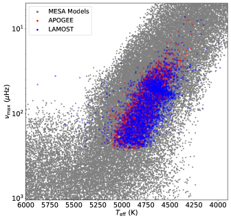
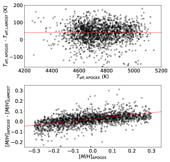
Figure 1: Left: The Kepler RGB stars on the $T_{\rm eff}$–$\nu_{\rm max}$ diagram. Grey dots are 50,000 MESA models randomly selected from our grid. Blue and red dots represent the 2,626 APOGEE and 3,326 LAMOST tragets. Observed $\nu_{\rm max}$ values are from Yu et al. (2018b). Right: Differences in effective temperature (upper) and metallicity (bottom) of the 1,825 common stars. Red dashes indicate the systematic offsets, which is constant ($T_{\rm eff,APOGEE}$ = $T_{\rm eff,LAMOST}$ + 41 K) for effective temperature and a linear function ([M/H]_APOGEE = 0.20[M/H]_LAMOST + 0.023 dex) for metallicty.

2.2 Measurement of Radial Oscillation Mode Frequencies

We first identified the radial modes for the aforementioned stars. The asymptotic relation for p modes can be used to predict the mode frequencies on the basis that modes of the same $l$-degree and sequential $n$ are separated by about $\Delta\nu$ (Tassoul, 1980; Gough, 1986):

$$\nu(n,l)=\Delta\nu\left(n+\frac{l}{2}+\epsilon\right)-\delta\nu_{0l},$$ (6)

where $\epsilon$ defines an offset and $\delta\nu_{0l}$ is the small spacing between modes of different $l$-degrees. We made use of this regularity to determine approximate locations of the radial modes, which means determining $\epsilon$ for each star. We used the background-corrected power spectra produced by Yu et al. (2018b) and selected data around $\nu_{\rm max}$ in a range of 5 times the FWHM (full width at half maximum) of the power excess. We then obtained the so-called collapsed power spectrum where the power was added from consecutive slices with width of $\Delta\nu$. This collapsed power spectrum was cross-correlated with a template comprising three peaks, constructed according to the asymptotic equation, corresponding to the ridges of $l=0$, 1 and 2 modes. We adopted a value for $\delta\nu_{0l}$ that was a fixed fraction of $\Delta\nu$, set by a fit to real stars (Huber et al., 2010). The value of $\epsilon$ was then obtained by maximising the correlation coefficient. The locations of radial modes were restricted to be in the region $(\nu_{n,l=0}/\Delta\nu\ {\rm mod}\ 1)\in[\epsilon-0.06,\epsilon+0.12]$. Fig. 2 shows this identification procedure for an example star, KIC 8410637.

Having located the radial modes, we fitted Lorentzian profiles to these regions to extract the radial mode frequencies:

$$M(\nu)=B(\nu)\cdot\eta^{2}(\nu)\cdot\sum_{n}L_{n}(\nu)=B(\nu)\cdot\frac{\sin^{2}(\pi\nu\Delta t)}{(\pi\nu\Delta t)^{2}}\cdot\sum_{n}\frac{A_{n}^{2}/(\Gamma_{n})}{1+4(\nu-\nu_{n})^{2}/\Gamma_{n}^{2}},$$ (7)

using the fitting method as described by Li et al. (2020b). We used an H1 (odds ratio) approach to evaluate the quality of each fit (Appourchaux et al., 2012; Corsaro & De Ridder, 2014; Davies et al., 2016b; Lund et al., 2017b). We retained those modes with a Bayes factor larger than $3$, equivalent to strong detection (Kass & Raftery, 1995). As an example, we listed model frequencies, uncertainties of KIC 8410637 in Table 1. This star is the red-giant component in a classified EB system. Its radial mode frequencies were previously measured by direct fitting (Li et al., 2018). The comparison shows that the model frequencies from our pipeline well agree with previous results and we find one extra mode at low frequency. We also found good consistencies in extracted modes for five other red-giants components studied by Li et al. (2018).

The number of identified radial modes is 6 on average, reaching up to 10 for low-luminosity RGB stars and decreasing with the evolution. For high-luminosity red giants with $\nu_{\rm max}$ below 20$\mu$Hz, most stars have only 3–4 modes. We note that a few of the stars may have incorrect results since they were returned from an automatic pipeline. They do not affect population studies because of their small number. However, to use frequencies for a particular star, they should carefully vetted. The source code for the mode measurement and lists of identified frequencies for the all stars are available on https://github.com/litanda/SolarlikePeakbagging.

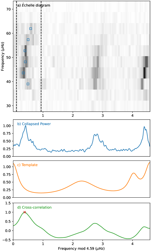
Figure 2: Measurement of radial modes for KIC 8410637. a) The power spectrum in échelle format. b) The collapsed power spectrum. c) The template spectrum. d) The cross-correlation spectrum between b) and c). The red cross shows the maximum in the cross-correlation spectrum, which gives the value of $\epsilon$ and identifies the ridge of radial modes. We used this to define the frequency ranges for the radial modes (shown as black dashed lines) and then fitted the strongest peaks within these ranges. The fitted frequencies are marked by squares.

Table 1: Extracted radial modes of an example star KIC 10513837.

$\nu$ ($\mu$Hz)	$\sigma_{\nu}$ ($\mu$Hz)	Ref.a
37.19	0.02	-
41.62	0.02	$41.63\pm 0.03$
46.28	0.02	$46.29\pm 0.03$
50.85	0.02	$50.86\pm 0.02$
55.55	0.06	$55.53\pm 0.05$
60.22	0.05	$60.37\pm 0.03$
a Mode frequencies from Li et al. (2018).

3 Theoretical Modeling

3.1 Model Grid and Input Physics

We constructed a stellar model grid that ranges from 0.76 to 2.20$M_{\odot}$ with a mass step of 0.02$M_{\odot}$. The grid includes four independent model inputs: stellar mass ($M$), initial helium fraction ($Y_{\rm init}$), initial metallicity ([M/H]), and the mixing-length parameter ($\alpha_{\rm MLT}$). Ranges and grid steps of these four model inputs are given in Table 2. We started computation of each stellar evolutionary track from the Hayashi line and terminated on the upper RGB when $\log g$ $\geq$ 1.5 dex. Note that we did not include models undergoing core helium burning.

Table 2: Input Ranges and Grid Step of the Model Grid.

Input Parameter	Range		Increment
	From	To
$M/$M⊙	$-$0.76	2.20	0.02
$\rm{[Fe/H]}$	$-0.5$0	0.50	0.10
$Y_{\rm init}$	$-$0.24	0.32	0.02
$\alpha_{\rm{MLT}}$	$-$1.70	2.50	0.20

We used the stellar evolution code mesa (Modules for Experiments in Stellar Astrophysics, version 12115, Paxton et al. 2011, 2013, 2015, 2018) and the oscillation code gyre (version 5.1, Townsend & Teitler 2013) to compute the model grid. We adopted the solar chemical mixture [$(Z/X)_{\odot}$ = 0.0181] provided by Asplund et al. (2009). The initial chemical composition was calculated by:

$$\log(Z_{\rm{init}}/X_{\rm{init}})=\log(Z/X)_{\odot}+\rm{[M/H]_{init}}.\\$$ (8)

We used the mesa $\rho$–$T$ tables based on the 2005 update of the OPAL equation of state tables (Rogers & Nayfonov, 2002) and OPAL opacities supplemented by the low-temperature opacities from Ferguson et al. (2005). The Eddington photosphere was used for the set of boundary conditions for modeling the atmosphere. The mixing-length theory of convection was applied, where $\alpha_{\rm MLT}=\ell_{\rm MLT}/H_{\rm p}$ is the mixing-length parameter. We considered convective overshooting at the core, the H-burning shell, and the envelope. The exponential scheme by Herwig (2000) was applied and the diffusion coefficient in the overshoot region given as

$${D_{\rm{OV}}}={D_{\rm{conv,0}}}\exp\left(-\frac{{2(r-r_{0})}}{{(f_{0}+f_{\rm{ov}}){H_{p}}}}\right).$$ (9)

Here, $D_{\rm{conv,0}}$ is the diffusion coefficient from the mixing-length theory at a user-defined location near the Schwarzschild boundary. The switch from convection to overshooting was set to occur at $r_{0}$. To consider the step taken inside the convective region, $(f_{0}+f_{\rm{ov}}){H_{\rm p}}$ was used, where $f_{\rm 0}$ equals 0.5$f_{\rm{ov}}$. Following Magic et al. (2010), the overshooting parameter is mass-dependent following a relation as $f_{\rm{ov}}=(0.13M-0.098)/9.0$, and a fixed $f_{\rm{ov}}$ of 0.018 was adopted for models above $M=2.0$ M_⊙. For a smooth convective boundary, we also applied the mesa predictive mixing scheme. The mass-loss rate on the red-giant branch with Reimers’ law was set as $\eta=0.2$, which is constrained by the seismic targets in old open clusters NGC 6791 and NGC 6819 (Miglio et al., 2012). Atomic diffusion was only considered for models below 1.1M_⊙ at the main-sequence phase (it is turned off when central hydrogen fraction goes below 0.01). As discussed by Mowlavi et al. (2012), the mass value of 1.1M_⊙ is a proper switching point, above which the surface helium and heavy elements would be rapidly drained out of the envelope if atomic diffusion were applied. The switch of atomic diffusion causes a discontinuity in the surface metallicity as well as other global parameters during the main-sequence and early subgiant stages, but most of the effects are not significant at the RGB phase due to the redistribution of star interiors (Michaud et al., 2010; Dotter et al., 2017). However, element diffusion also changes the main-sequence lifetime and hence a discontinuity in star age is expected for the RGB models at 1.1 M_⊙ (e.g. Fig. 11 Mowlavi et al., 2012). To investigate the systematic uncertainty, we compared stellar ages at given mean density on RGB for evolutionary tracks with and without atomic diffusion. The comparisons shows an 8% difference for 1.1M_⊙ evolutionary tracks. The age difference is strongly mass-dependent, going down to 1% at 1.2M_⊙ and is approximately zero at 1.3M_⊙. We hence expect a systematic uncertainty of a few per cent in inferred ages in the mass range of 1.1–1.2 M_⊙. Compared with the typical uncertainty (16%), our estimated ages for stars about 1.1M_⊙ could be biased to some extent for the choice of atomic diffusion, but this systematic difference is negligible above 1.2 M_⊙.

3.2 Fitting Method

We used the Maximum Likelihood Estimate (MLE) method for fitting the models to the observations. In Figure 3, we demonstrate our fitting procedure with the example star. We first searched for models in the range 0.8–1.2 times $\Delta\nu$. Note that the $\Delta\nu$ scaling relation was used in this step and the $\pm$20% range was large enough to cover its systematic uncertainty. We fitted the observed $T_{\rm eff}$ and [M/H] to models and calculated the non-seismic likelihood ($L_{\rm non-seismo}$) with the following equation:

$$L_{\rm non-seismo}={\rm exp}\left[-\frac{(T_{\rm eff,obs}-T_{\rm eff,mod})^{2}}{2\sigma^{2}_{T_{\rm eff,obs}}}-\frac{([M/H]_{\rm obs}-[M/H]_{\rm mod})^{2}}{2\sigma^{2}_{[M/H]_{\rm obs}}}\right],\\$$ (10)

where the subscripts ‘obs’ and ‘mod’ stand for the observed and model values. Note that, because our grid resolution for [M/H] is 0.1 dex, an uncertainty of $\pm$0.1 for [M/H] was used when a star’s observed uncertainty is smaller than this value. We selected models with $L_{\rm non-seismo}>0.0001$ for the subsequent seismic analysis.

We corrected the surface term in oscillation frequencies of each selected model using the two-term formula given by Ball & Gizon (2014). While inspecting the fits of frequencies, we noticed that some bad models whose frequencies deviated strongly from the observations could be made to fit well after an implausibly large surface correction. To avoid this, we set up a threshold for the surface term when selecting models for the seismic fitting. Although the surface term of a certain model is unknown before fitting, we can learn from previous studies to roughly estimate its range. According to results on Kepler main-sequence and RGB stars (Compton et al., 2018; Li et al., 2018, 2021), relative surface corrections at $\nu_{\rm max}$ ($\delta\nu_{\rm corr}$($\nu_{\rm max}$)/$\nu_{\rm max}$) for most stars are in a range from $-0.005$ to $-0.01$. Considering the potential systematic differences between theoretical models, we used a larger range as the threshold, namely 0 to 0.02. After correcting the surface term, we checked the relative surface corrections at $\nu_{\rm max}$ and only kept models fitting this threshold criterion.

We next fitted individual radial mode frequencies and calculated a seismic likelihood of each model for as

$$L_{\rm seismo}=\prod{\rm exp}\left[-\frac{(\nu_{i\rm,obs}-\nu_{i\rm,mod})^{2}}{2(\sigma^{2}_{\nu_{i\rm,obs}}+\sigma^{2}_{\nu_{\rm sys}})}\right].\\$$ (11)

The subscript $i$ refers to the mode frequencies. As discussed by Li et al. (2020a), the systematic uncertainty in model frequencies cannot be neglected in the detailed modeling because it could be comparable to or larger than the observed uncertainty. For this reason, the fit was done in two steps. In the first step, we only considered the observed frequency uncertainty ($\sigma_{\nu,obs}$) in the likelihood function and found the best-fitting model. We used the median value of frequency offsets between the observations and this best-fitting model as the systematic uncertainty ($\sigma_{\rm sys}$). In the second step, we fitted to individual mode frequencies again but included the $\sigma_{\rm sys}$ term in the likelihood function. Multiplying the non-seismic and seismic likelihoods gave us the final likelihood as $L=L_{\rm non-seismo}\cdot L_{\rm seismo}$. We used the marginal likelihood distribution to measure the 16%, 50% and 84% cumulative values to determine global parameters (i.e., mass, age, radius, surface gravity, and luminosity) and their uncertainties.

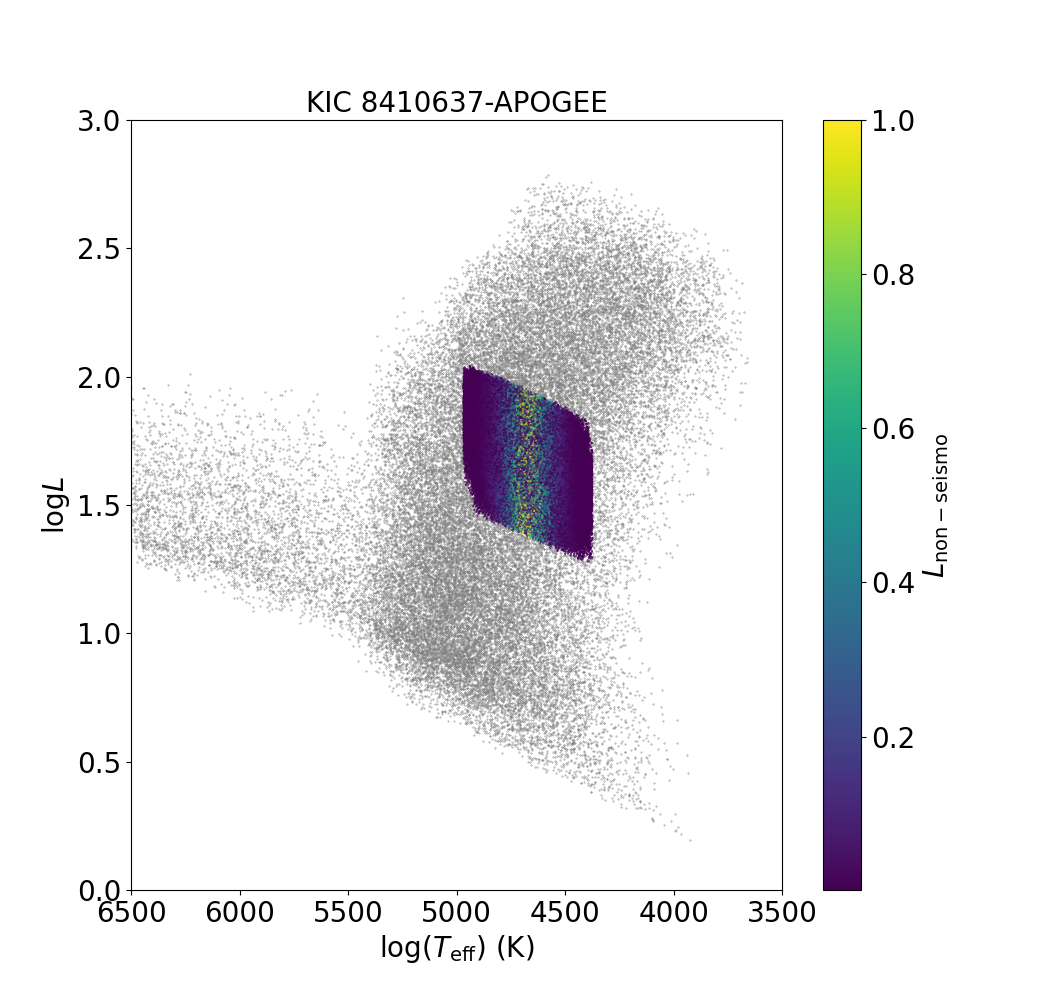
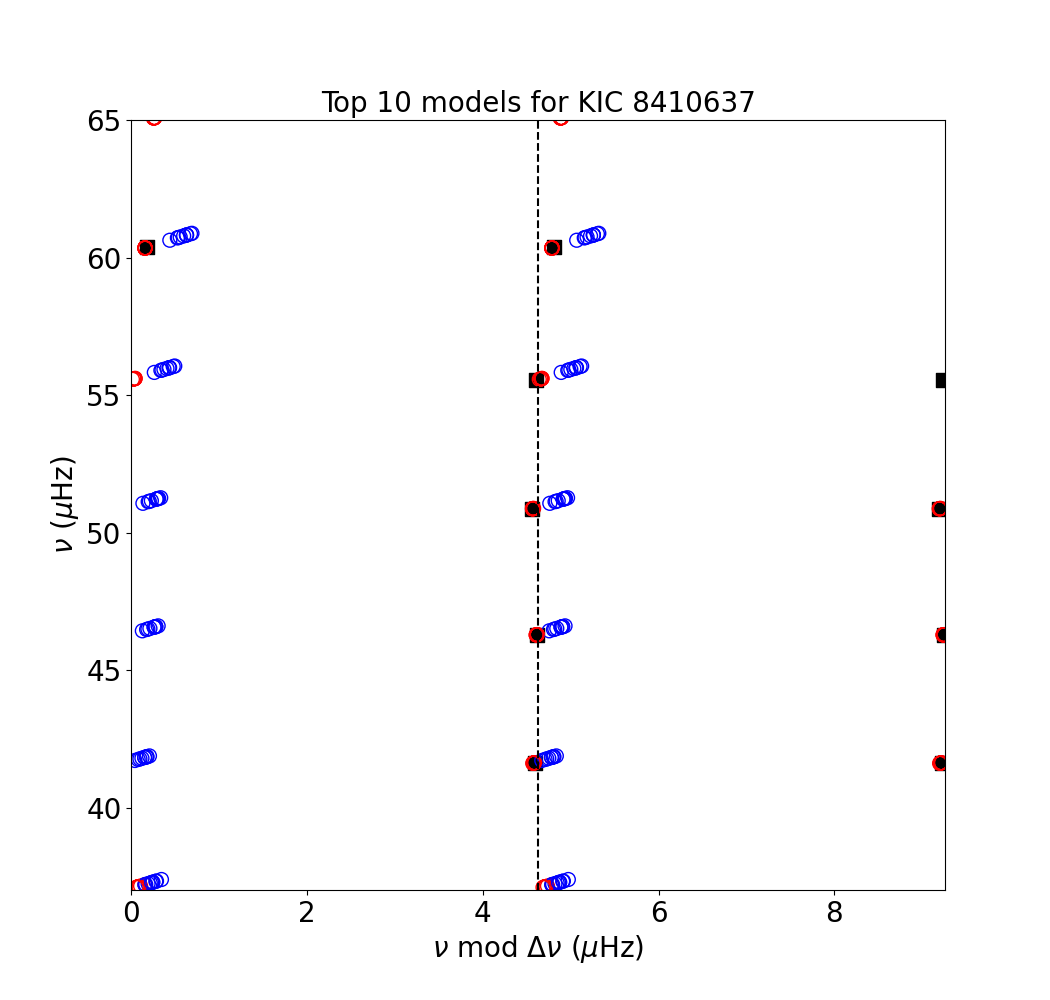
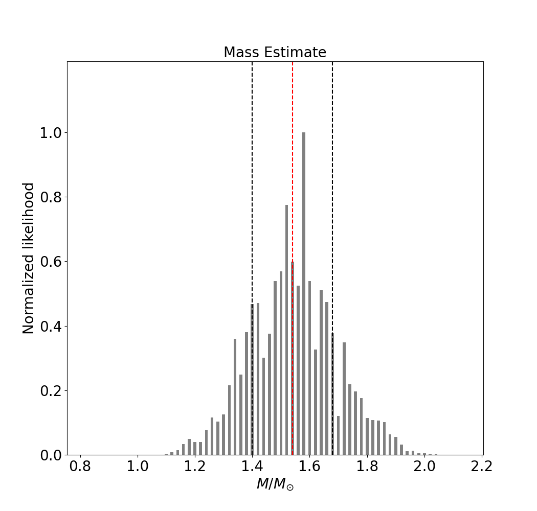
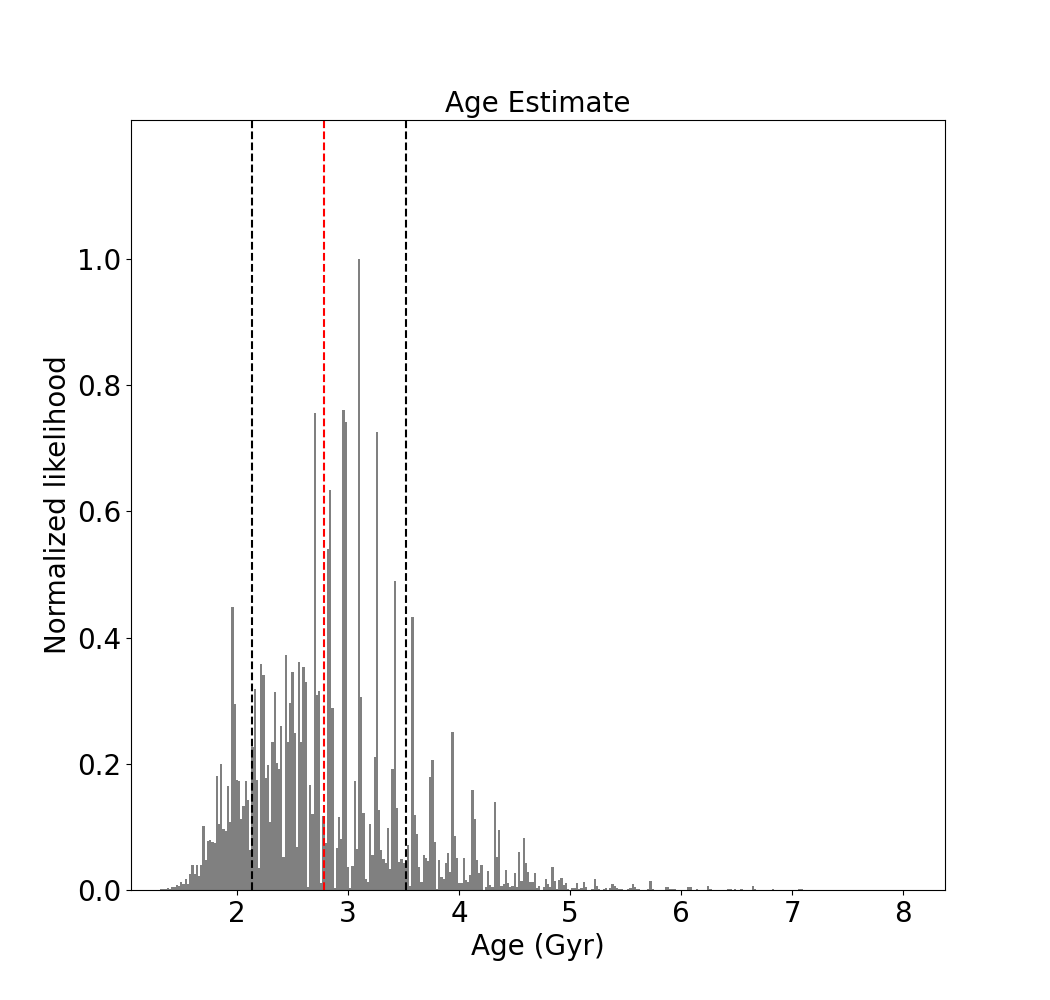
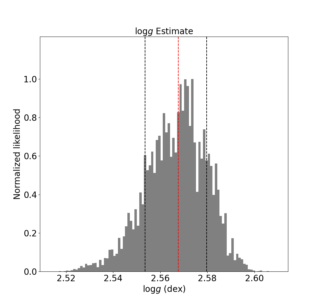
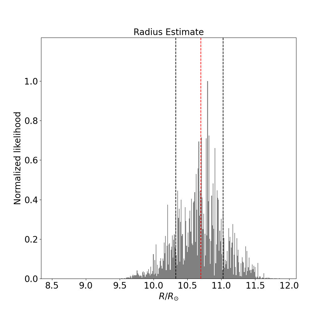
Figure 3: The fitting procedure for the example star (KIC 8410637). Top left: Fitting models to spectroscopic constraints ($T_{\text{eff}}$ and [M/H]) in the range 0.8–1.2 $\Delta\nu$ and selecting those with $L_{\rm non-seismo}>0.0001$ for the subsequent seismic analysis. Grey dots represent the all models, colour-coded dots are selected models and colour indicates the non-seismic likelihood ($L_{\rm non-seismo}$). Top right: Fitting observed mode frequencies. We demonstrate the fits on the échelle diagram. Filled black squares are observed mode frequencies, open blue and red circles represent theoretical mode frequencies before and after the surface correction. The échelle diagram is plotted twice to fully present the radial mode pattern, and the blue dashed line indicates the large separation. Middle and bottom rows: probability distributions for mass, age, surface gravity, and radius. The central red dashed line indicates the median of each distribution, and two black dashed lines mark the 16% and the 84% cumulative values (1-$\sigma$ uncertainty).

4 Results

4.1 Five Red Giants in Eclipsing Binaries

The accuracy of estimated masses and radii is critical because we use them to calibrate the scaling relations. We hence examined the accuracy of modeling solution with five red giants in EB systems, whose masses and radii have been previously determined with dynamical modeling. We found APOGEE spectra available for all five red giants and LAMOST data for three of them. The comparison is demonstrated in Figure 4. We used the dynamical results determined by Frandsen et al. (2013), Gaulme et al. (2016) and Brogaard et al. (2018), and the average value was taken when there was more than one estimate for the same star. With the APOGEE spectra, our model-based masses and radii agree within $1\sigma$ for three out of the five stars, $1.5\sigma$ for KIC 9970396, and $2\sigma$ for KIC 4663623. The reason for the large offset on KIC 4663623 could be the very different metallicities adopted in our fitting (${\rm[M/H]}=0.08$) and the dynamical modeling (${\rm[M/H]}=-0.13$). Estimates for the three stars with the LAMOST data are slightly more discrepant but still consistent with dynamical determinations. In Table 3, we summarise estimated masses and radii given by the detailed modeling, the scaling relations, and dynamical analysis. Compared with the scaling relation, the fits to radial mode frequencies significantly improve the accuracy of mass and radius estimates.

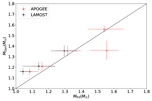
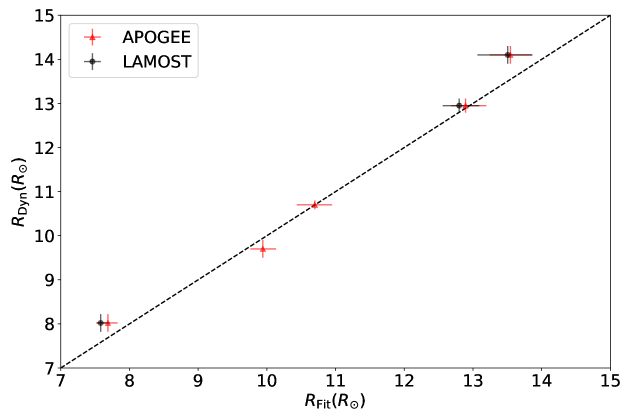
Figure 4: Masses and radii determined by fitting radial modes versus those from dynamical modeling, for five red giants in EB systems. The black dashed lines show the 1:1 relation.

Table 3: Masses and radii of five red giants in EB systems derived from our modeling, the scaling relations, and dynamical modeling.

KIC	$M_{\rm Fit}$	$R_{\rm Fit}$	$M_{\rm SR}$	$R_{\rm SR}$	$M_{\rm Dyn}$	$R_{\rm Dyn}$	Ref.
	(M⊙)	(R⊙)	(M⊙)	(R⊙)	(M⊙)	(R⊙)
4663623	$1.56^{+0.10}_{-0.12}$	$9.94^{+0.20}_{-0.25}$	1.87$\pm$0.13	10.78$\pm$0.28	1.36$\pm$0.09	9.7$\pm$0.2	G16
7037405	$1.16^{+0.08}_{-0.08}$	$13.55^{+0.37}_{-0.31}$	$1.38\pm 0.10$	$14.76\pm 0.41$	$1.25\pm 0.04$	$14.1\pm 0.2$	G16
					$1.170\pm 0.020$	$14.000\pm 0.093$	B18
8410637	$1.54^{+0.14}_{-0.14}$	$10.70^{+0.33}_{-0.37}$	$1.78\pm 0.19$	$11.45\pm 0.56$	$1.56\pm 0.03$	$10.7\pm 0.1$	F13
9540226	$1.32^{+0.08}_{-0.08}$	$12.89^{+0.25}_{-0.28}$	$1.58\pm 0.11$	$14.05\pm 0.37$	$1.33\pm 0.05$	$12.8\pm 0.1$	G16
					$1.378\pm 0.038$	$13.060\pm 0.160$	B18
9970396	$1.08^{+0.06}_{-0.06}$	$7.69^{+0.15}_{-0.16}$	$1.43\pm 0.08$	$8.68\pm 0.17$	$1.14\pm 0.03$	$8.0\pm 0.2$	G16
					$1.178\pm 0.015$	$8.035\pm 0.074$	B18

References: F13 – Frandsen et al. (2013), G16 – Gaulme et al. (2016), B18 – Brogaard et al. (2018)

4.2 Estimated Stellar Parameters

We used the fitting method described in Section 3.2 to estimate stellar parameters (mass, age, surface gravity, and radius) for the 4,127 Kepler RGB stars. We first removed three types of stars from final results: i) stars with three or fewer identified radial modes, because the fits will largely affected by the uncertainty in surface correction; ii) stars with estimated masses below 0.85 or above 2.10 M_⊙, because those values are close to the edge of the grid; iii) stars with fewer than 100 models for the seismic analysis, because their observed constraints are either close to the edge or outside the parameter ranges of the model grid. We then examined age determinations to identify those targets with unrealistically large estimates. These targets may bias the calibration for the scaling relation, given that age correlates strongly with mass for RGB stars. We found 61 out of 5,350 estimated ages that are larger than the universe age (13.8 Gyr) by more than 2-$\sigma$. We inspected those targets and found some of them do not have reliable $T_{\text{eff}}$ measurements and others could be core-helium-burning stars according to their power spectra. The fraction ($\sim 1.1\%$) of poor age determinations generally agrees with the accuracy rate of classifications reported by Hon et al. (2017). We then removed the targets with poor age estimates from the sample. We finally obtained 5,289 modeling solutions for 3,642 stars, including 2,498 APOGEE and 2,791 LAMOST targets with 1,647 common sources. We list observed constraints and estimated parameters in Table 4 (the full table is included in the supplement).

Table 4: Observed constraints and model-inferred stellar parameters (full table available on-line).

	Observed Constraints					Estimates
KIC	Source	$T_{\rm eff}$	[M/H]	$\Delta\nu$	$\nu_{\rm max}$	$M$	$\tau$	$R$	$\log g$
		(K)	(dex)	($\mu$Hz)	($\mu$Hz)	($M_{\odot}$)	(Gyr)	($R_{\odot}$)	(dex)
8161920	APOGEE	4551	-0.046	3.65	31.9	$1.14^{+0.08}_{-0.08}$	$7.7^{+3.3}_{-1.5}$	$11.26^{+0.22}_{-0.33}$	$2.393^{+0.007}_{-0.011}$
5358184	APOGEE	4632	0.104	6.23	62.4	$1.14^{+0.02}_{-0.03}$	$9.7^{+1.2}_{-1.8}$	$7.87^{+0.08}_{-0.09}$	$2.701^{+0.004}_{-0.004}$
10793872	APOGEE	4780	-0.229	14.86	181.7	$0.94^{+0.03}_{-0.04}$	$14.6^{+2.9}_{-1.0}$	$4.19^{+0.04}_{-0.09}$	$3.17^{+0.003}_{-0.008}$
8815290	APOGEE	4821	-0.112	4.46	45.5	$1.72^{+0.10}_{-0.16}$	$1.9^{+0.5}_{-0.3}$	$11.38^{+0.25}_{-0.37}$	$2.56^{+0.008}_{-0.012}$
7749249	APOGEE	4703	0.099	6.66	71.8	$1.22^{+0.08}_{-0.04}$	$5.1^{+1.2}_{-0.7}$	$7.72^{+0.17}_{-0.11}$	$2.751^{+0.007}_{-0.007}$
8161920	LAMOST	4560	0.249	3.65	31.9	$1.14^{+0.08}_{-0.04}$	$8.6^{+2.5}_{-1.5}$	$11.25^{+0.23}_{-0.19}$	$2.394^{+0.006}_{-0.007}$
5358184	LAMOST	4573	-0.018	6.23	62.4	$1.14^{+0.02}_{-0.02}$	$9.08^{+1.9}_{-0.9}$	$7.87^{+0.06}_{-0.05}$	$2.702^{+0.001}_{-0.003}$
10793872	LAMOST	4925	0.110	14.86	181.7	$0.94^{+0.03}_{-0.04}$	$16.2^{+1.4}_{-2.6}$	$4.16^{+0.07}_{-0.06}$	$2.17^{+0.005}_{-0.006}$
8815290	LAMOST	4749	-0.195	4.46	45.5	$1.68^{+0.12}_{-0.14}$	$2.4^{+0.4}_{-0.5}$	$11.26^{+0.31}_{-0.33}$	$2.558^{+0.010}_{-0.009}$
7749249	LAMOST	4681	0.117	6.66	71.8	$1.24^{+0.08}_{-0.06}$	$4.8^{+1.2}_{-0.5}$	$7.76^{+0.17}_{-0.14}$	$2.752^{+0.007}_{-0.007}$

To inspect the precision of inferred parameters, we show histograms of the uncertainties in Figure 5. We obtained similar average precision for the LAMOST and APOGEE samples, but the LAMOST sample spreads over a larger range. The typical precision (the median of the distribution) for both samples is 4.5% for mass, 16% for age, 0.006 dex for $\log g$, and 1.7% for radius.

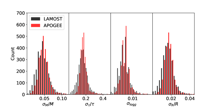
Figure 5: Fractional uncertainties of the estimated parameters for stars with LAMOST and APOGEE spectroscopic constraints.

We compared inferred values determined with the APOGEE and the LAMOST spectra to investigate any systematic differences caused by the spectroscopy. In Figure 6, we illustrate comparisons for the 1,655 common targets and find good consistency at the sample level: the average differences for the four parameter are all around zero, with standard deviations that are similar to the typical uncertainties. The large offsets on some stars are due to the very different effective temperatures given by the two surveys. The results indicate that our fits are mainly determined by seismic mode frequencies, while the effective temperature and metallicity are relatively weak constraints.

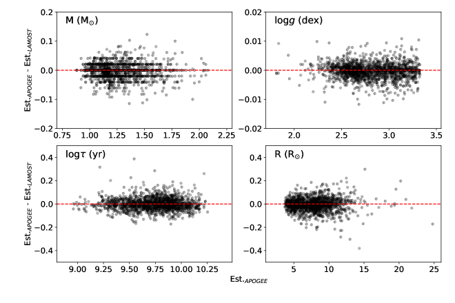
Figure 6: Comparisons between estimated parameters with LAMOST and APOGEE spectroscopic constraints. (In the top left panel, some data points present stripe-like features. These stars are low-luminous red giants, whose mass loss is negligible, and hence their estimated masses are about the same as the initial masses, which are uniformly spaced. Other high-luminous stars have signficant mass loss, and hence their inferred masses distribute more randomly.)

5 The scaling relations for red giants

Our model-based masses and radii of the Kepler RGB star sample can allow testing of the scaling relations over a wide parameter range. We have shown that our estimates for stellar masses and radii are accurate, and hence they are good reference values for correcting the scaling relations. We start by inspecting the ratio between the modeling determinations and the scaling relations. As illustrated in Figure 7, we find that the scaling relations overestimate masses and radii for most of the stars. The density distributions give median factors of $\sim$85% for the mass and $\sim$93% for the radius. These values are consistent with those found for EBs (Gaulme et al., 2016; Brogaard et al., 2018; Themeßl et al., 2018). In Figure 7, we see that the ratio weakly depends on mass and this may correspond to some systematic offset caused by the effective temperature or the metallicity. On the other hand, the ratio clearly varies with stellar radius, indicating the discrepancy depends on the evolutionary phase.

We wish to correct the scaling relations by combining the modeling solution and observations. Rather than correcting Eq. 3 and 4 directly, we prefer to work with the $\nu_{\rm max}$ and the $\Delta\nu$ scaling relations because they are more fundamental. The scaling relation for $\nu_{\rm max}$ is based on the assumption that $\nu_{\rm max}$ in solar-like oscillators is a fixed fraction of $\nu_{ac}$(Brown et al., 1991; Kjeldsen & Bedding, 1995). The acoustic cutoff frequency ($\nu_{ac}$) is the frequency above which acoustic waves are not reflected at the surface and it depends on the effective temperature and the surface gravity as $\nu_{ac}\propto gT_{\rm eff}^{-0.5}$. Regarding the $\Delta\nu$ scaling relation, the large frequency separation $\Delta\nu$ in the asymptotic approximation equals the inverse of the sound travel time through the star, which results in $\Delta\nu\propto\sqrt{M/R^{3}}$ (Ulrich, 1986). The $\Delta\nu$ value is hence proportional to the square root of the mean density ($\overline{\rho}$) of the star.

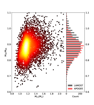
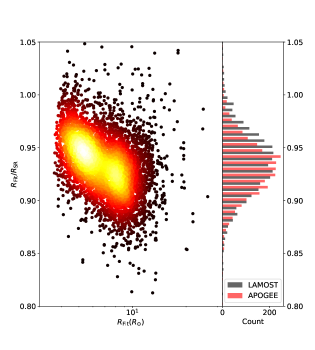
Figure 7: Ratios between estimated masses and radii from our modeling and from the scaling relations. Histograms show the stars with spectroscopic constraints from LAMOST and APOGEE.

5.1 Correcting the $\nu_{\rm max}$ Scaling Relation

We calculated the scaling $\nu_{\rm max}$ using model $T_{\rm eff}$ and $\log g$, and used the same fitting method to constrain it. We refer to this estimated scaling $\nu_{\rm max}$ as $\nu_{\rm max,SR}$. Note that we did not use the measured $\nu_{\rm max}$ as an input constraint in the fitting, and hence the determination of $\nu_{\rm max,SR}$ is independent of the observed value.

From the comparison between observed $\nu_{\rm max}$ and $\nu_{\rm max,SR}$, as demonstrated in Figure 8a, we find no significant systematic offset. However, the scatter (the standard deviation is $\pm$2.5%) is much larger the typical observed uncertainty, indicating potential dependencies on other stellar parameters or that $\nu_{\rm max}$ uncertainties are substantially underestimated. We therefore investigated the correlations with $\log g$, $T_{\rm eff}$, and [M/H] in Figures 8b, 8c, and 8d. The reason to consider the metallicity is that it could impact near-surface properties of solar-like oscillators, as suggested by hydrodynamic simulations (e.g. Trampedach et al., 2014). We see that the $\nu_{\rm max}$ offset does not obviously depend on $\log g$, but clearly correlates with $T_{\rm eff}$ and [M/H]. The same trend is seen in both the APOGEE and LAMOST samples. From the perspective of physics, the correlations with the effective temperature may be real because the thermal structures at the near-surface region are very different between RGB and main-sequence stars, although there is no theory that quantifies the difference in $T_{\text{eff}}$-$\nu_{\rm max}$ relations between the two types of stars. However, we suspect that this correlation is caused by the systematic offsets in the spectroscopic measurements because the dependency on $T_{\text{eff}}$ is slightly stronger for the LAMOST data than for the APOGEE data. The same applies for the metallicity, in that the correlation is likely a combination of the physical and the instrumental effects and we cannot separate them because of the lack of theoretical predictions. We will leave this as an open question for future studies.

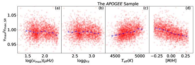
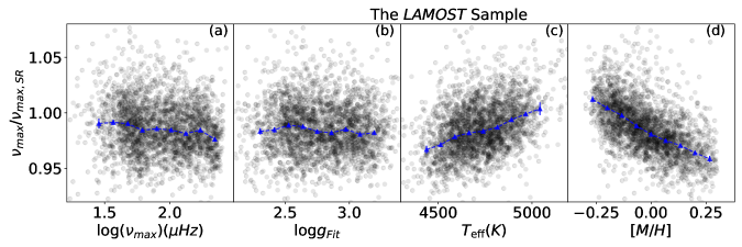
Figure 8: Dependencies of systematic offsets in $\nu_{\rm max}$ ($\nu_{\rm max}$/$\nu_{\rm max,SR}$) on $\nu_{\rm max}$, $T_{\rm eff}$, $\log g$,and [Fe/H]. The APOGEE sample is presented on the top and the LAMOST sample is shown at the bottom. Filled triangle is the median of binned data and the error bar indicates the the standard error of the median, which is calculated as the standard deviation over the number of data point in a bin ($\sigma/n$).

To correct for the systematics discussed above, we added a metallicity term to the $\nu_{\rm max}$ scaling relation. We calibrated the revised $\nu_{\rm max}$ scaling relation with model-based $\log g$, observed $\nu_{\rm max}$, $T_{\text{eff}}$, and [M/H]. We used the Scipy curve_fit module to do the fits and obtained corrected $\nu_{\rm max}$ scaling relations as follows:

$$\frac{\nu_{\rm max}}{\nu_{\rm max,\odot}}=\frac{g_{\rm Fit}}{g_{\odot}}\left(\frac{T_{\rm eff}}{T_{\rm eff,\odot}}\right)^{-0.459}\left(10^{\rm[M/H]}\right)^{-0.022}(\emph{APOGEE})\\ \\$$ (12)

and

$$\frac{\nu_{\rm max}}{\nu_{\rm max,\odot}}=\frac{g_{\rm Fit}}{g_{\odot}}\left(\frac{T_{\rm eff}}{T_{\rm eff,\odot}}\right)^{-0.421}\left(10^{\rm[M/H]}\right)^{-0.039}(\emph{LAMOST}).\\$$ (13)

We obtained the same power law for the $g$ term as the original relation, but the exponent of $T_{\rm eff}$ is slightly different from the original ($-0.5$). As discussed above, the difference does not necessarily mean that the RGB stars have a different $T_{\text{eff}}$–$\nu_{\rm max}$ relation from the dwarfs. For instance, when we considered a global temperature shift of $-70K$ in the APOGEE sample, as found by Hall et al. (2019), the fit gave a very similar power law to the original scaling relation. The additional term of [M/H] is a secondary term in the formulae, which causes a $\sim$4% change to the $\nu_{\rm max}$ value when [M/H] varies from -0.3 to 0.3 dex. Note that the LAMOST [M/H] values are based on the [Fe/H] and [$\alpha$/Fe] measurements. The choice of formula may bring some systematic uncertainties and we hence tested the fits with another widely-used formula, namely [M/H] = [Fe/H] + [$\alpha$/Fe]. The [M/H] values from this formula are higher than those calculated with Eq. 5 by 0.02 dex, on average, which is significantly smaller than the typical observed uncertainty. Fitting the scaling relation with these [M/H] values returns very similar results to Eq. 13. The exponent is $-0.427$ for the $T_{\text{eff}}$ term and 0.040 for the [M/H] term. The similarity indicates the choice of [M/H] formula does not significantly affect the new scaling relation.

5.2 The $\Delta\nu$ Scaling Relation

We studied the $\Delta\nu$ scaling relation following the same strategy. We used the mean density of models to calculate the large frequency separation from the scaling relation (Eq. 1) and constrained it based on model fitting. We refer to this as $\Delta\nu_{\rm SR}$. We first examined the systematic difference between observed $\Delta\nu$ and $\Delta\nu_{\rm SR}$. Note that the observed $\Delta\nu$ is from Yu et al. (2018b) rather than from individual radial modes. As shown in Figure 9a, there is a $\sim$4% deviation on average, and the offset varies from $-6$% to $-2$%. We then inspected the dependencies of $\Delta\nu$/$\Delta\nu_{\rm SR}$ on the mean density, effective temperature, and metallicity, as demonstrated in Figures 9b, 9c, and 9d.

The ratio clearly correlates with mean density and also with the effective temperature, and slightly depends on the metallicity. It is not clear which parameter has the true effect because these three parameters are correlated on RGB. As for its physical significance, we note that $\Delta\nu$ is determined by the mean density rather than by any surface properties. As pointed out by Miglio et al. (2012), the differences in internal temperature (hence sound speed) distributions could cause a noticeable difference in $\Delta\nu$ between different type of stars, despite them having the same mean density. Their comparison between hydrogen-shell-burning and helium-core-burning stars with similar mean densities in Kepler open clusters presented a $\sim$3.3% difference in average $\Delta\nu$. As a consequence, the difference in $\Delta\nu$–$\rho$ scaling relation between RGB and main-sequence stars is expected because of their different internal structures. The correlations with effective temperate and metallicity arise because these two surface properties relate to the mean density: for stars on RGB, the effective temperature strongly correlates with mass, and hence with mean density, at given radius. Moreover, high-resolution spectroscopic surveys have shown a clear $T_{\text{eff}}$–[M/H] relation on the RGB (e.g. Fig.2 Tayar et al., 2017). For this reason, we retained the functional form of $\Delta\nu$ scaling relation and did not include the effective temperature or the metallicity in the new scaling relation.

We calibrated the $\Delta\nu$–$\rho$ scaling relation using observed $\Delta\nu$ and modeling-inferred mean density ($\rho_{\rm Fit}$), obtaining the following results:

$$\frac{\Delta\nu}{\Delta\nu_{\odot}}=\left(\frac{\overline{\rho}_{\rm Fit}}{\overline{\rho}_{\odot}}\right)^{0.507}.\\$$ (14)

Note that this function is for both the APOGEE and LAMOST samples because there is no systematic differences in inferred mean densities between the two at the sample level. Compared with the scaling for $\nu_{\rm max}$, the scaling for $\Delta\nu$ has a significantly larger systematic offset and the corrections are especially important for RGB stars. The correction to the $\Delta\nu$ scaling relation also matches the evolution-dependent systematic offsets found in previous studies (e.g. Sharma et al., 2016). We see that the power law exponent relating the large separation and the mean density for RGB stars is larger than that for dwarfs. This causes $\Delta\nu$ offsets (in fractional terms) to grow exponentially with decreasing $\Delta\nu$, and hence leads to larger systematic offsets for more evolved stars. We also note that a departure from the 0.5 exponent in the $\Delta\nu$ scaling relation has also been seen in $\delta$ Scuti stars (e.g., García Hernández et al., 2015; Bedding et al., 2020).

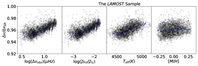
Figure 9: Same as Figure 8 but for $\Delta\nu$.

Our correction to the $\Delta\nu$ scaling relation is similar to previous studies by White et al. (2011) and Sharma et al. (2016), who checked whether the $\Delta\nu$ from fitting the model frequencies matched the value from the scaling the model density. This work is an improvement on that earlier work in that our corrections include the surface correction to model frequencies. It would be useful to investigate how much the surface term affect the corrections $\Delta\nu$ scaling relation. To do this, we followed the method described by White et al. (2011) and Sharma et al. (2016) to calculate the correction factor, $f_{\Delta\nu}$. In line with their notation, we defined our $\Delta\nu$ corrections as $f\,^{\prime}_{\Delta\nu}$ = $\Delta\nu$/$\Delta\nu$_SR. With this notation, we can re-write Eq. 14 as

$$\frac{\Delta\nu}{\Delta\nu_{\odot}}=f\,^{\prime}_{\Delta\nu}\left(\frac{\overline{\rho}_{\rm Fit}}{\overline{\rho}_{\odot}}\right)^{0.5}.\\$$ (15)

Here, $f\,^{\prime}_{\Delta\nu}$ can be taken as an improved version of $f_{\Delta\nu}$, with an additional correction for the surface term. Figure 10 shows the comparison between $f_{\Delta\nu}$ and $f\,^{\prime}_{\Delta\nu}$ of the best-fitting models for all stars. The differences are roughly uniform and the average differences are 1.6% and 1.4% for the APOGEE and LAMOST samples, respectively. If we adopt a 1.5% difference in the $\Delta\nu$ correction factor and transfer this difference to the mass and radius determinations, the surface term will cause a systematic offset of $\sim$6% for the mass and $\sim$3% for the radius, which are highly significant. We hence conclude that the surface term is worthy of attention in the corrections to the $\Delta\nu$ scaling relation.

The surface term depends on properties of near-surface layers and we hence inspected its correlations with the mean density, effective temperature, and metallicity. As shown in Figure 11, the difference between the two factors decreases with $\Delta\nu$, implying that the surface term is smaller for more evolved stars. This trend is consistent with 3D convection simulations of the surface effect on the RGB (e.g. Trampedach et al., 2017). The effective temperature also has an effect on the surface term according to those simulation results, but it is not obvious in our sample because the effective temperature range on RGB is fairly narrow. We also notice a rough correlation with the metallicity. This is expected because the metallicity can also change the convection properties at near surface Magic et al. (e.g. 2015).

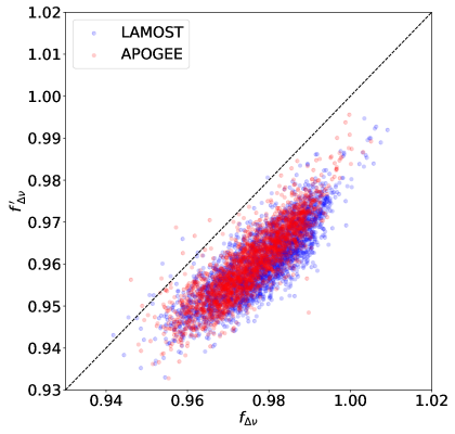
Figure 10: The comparison between the two correction factors to the $\Delta\nu$ scaling relation ($f_{\Delta\nu}$ and $f\,^{\prime}_{\Delta\nu}$) for the APOGEE sample. Here, $f\,^{\prime}_{\Delta\nu}$ can be taken as the an improved version of $f_{\Delta\nu}$ due to an additional correction for the surface term.

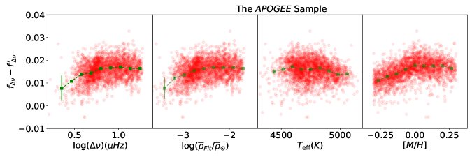
Figure 11: The difference in the two correction factors to the $\Delta\nu$ scaling relation ($f\,^{\prime}_{\Delta\nu}$ - $f_{\Delta\nu}$) as a function of four stellar parameters for the APOGEE sample. Green squares indicates the rolling median of the data. Results for the LAMOST sample (not shown) are similar.

5.3 Corrected Scaling Relations for Red Giants

With corrected $\nu_{\rm max}$ and $\Delta\nu$ scaling relations (Eq. 12, 13 and 14), we derived new scaling relations for determining stellar masses and radii. For the APOGEE sample they are:

$$\frac{M_{\rm Fit}}{M_{\odot}}=\left(\frac{\nu_{\rm max}}{\nu_{\rm max,\odot}}\right)^{3.0}\left(\frac{\Delta\nu}{\Delta\nu_{\odot}}\right)^{-3.944}\left(\frac{T_{\rm eff}}{T_{\rm eff,\odot}}\right)^{1.377}\left(10^{\rm[M/H]}\right)^{0.066},$$ (16)

and

$$\frac{R_{\rm Fit}}{R_{\odot}}=\left(\frac{\nu_{\rm max}}{\nu_{\rm max,\odot}}\right)\left(\frac{\Delta\nu}{\Delta\nu_{\odot}}\right)^{-1.972}\left(\frac{T_{\rm eff}}{T_{\rm eff,\odot}}\right)^{0.459}\left(10^{\rm[M/H]}\right)^{0.022}.$$ (17)

For the LAMOST sample they are:

$$\frac{M_{\rm Fit}}{M_{\odot}}=\left(\frac{\nu_{\rm max}}{\nu_{\rm max,\odot}}\right)^{3.0}\left(\frac{\Delta\nu}{\Delta\nu_{\odot}}\right)^{-3.944}\left(\frac{T_{\rm eff}}{T_{\rm eff,\odot}}\right)^{1.263}\left(10^{\rm[M/H]}\right)^{0.117},$$ (18)

and

$$\frac{R_{\rm Fit}}{R_{\odot}}=\left(\frac{\nu_{\rm max}}{\nu_{\rm max,\odot}}\right)\left(\frac{\Delta\nu}{\Delta\nu_{\odot}}\right)^{-1.972}\left(\frac{T_{\rm eff}}{T_{\rm eff,\odot}}\right)^{0.421}\left(10^{\rm[M/H]}\right)^{0.039}.$$ (19)

It worth noting that the above relations are only valid for RGB stars within a parameter range of $T_{\rm eff}=4400$ to 5200 K, $\nu_{\rm max}=10$ to 270 $\mu$Hz, and ${\rm[M/H]}=-0.3$ to 0.3 dex. We suggest caution when applying them outside these parameter ranges.

As a test, we computed masses and radii with the new scaling relations and compared them with model-determined values. We illustrate the distributions of the residuals in Figure 12. The distributions center at zero with a Half-Width-at-Half-Maximum of $\sim$5% for the mass and of $\sim$2% for the radius. These are consistent with the typical estimated uncertainties, which are 4.5% and 1.7% for mass and radius.

Because the new scaling relations are based on modeling solutions, some systematic uncertainties are expected. We considered reasonable ranges for the helium fraction and the mixing-length parameter, so the systematic effects from these two inputs are covered in the estimated uncertainty. However, the choices of other input physics could bias the results to some extent. These include the solar composition, the opacity, the atmosphere boundary condition, mass-loss rate, and atomic diffusion. The systematic offset, according to comparisons between seven different pipelines for Kepler main-sequence stars (Silva Aguirre et al., 2017), is about $\sim$2% for the mass and $\sim$1% for the radius on average. Systematic offsets related to input physics in our work could be different because internal structures of RGB stars are very different from those of dwarfs. Future studies are required to properly estimate the model systematic uncertainties.

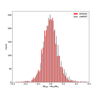
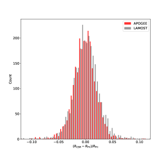
Figure 12: Differences between modeling-inferred results and corrected scaling relations (represented by the subscript ‘CSR’). Both density distributions center around zero with a standard deviation of $\sim 5\%$ for mass and $\sim 2\%$ for radius.

We calibrated scaling relations for the APOGEE and LAMOST samples separately because of the systematic differences in their measurements. Given the large number of APOGEE and LAMOST spectra, the new scaling relations should be useful for future studies. It is also worth considering whether to apply these new scaling relations to stars observed by other spectroscopic surveys. To test this, we applied the APOGEE formulae to the LAMOST data. As determined from Figure 1, we uniformly increased the LAMOST $T_{\text{eff}}$ by 44K, and calibrated the LAMOST [M/H] using the linear function as 0.20[M/H] + 0.023. We used calibrated LAMOST $T_{\text{eff}}$ and [M/H] in Eq. 16 and 17 to calculate masses and radii. Comparing with model-based determinations, we found good consistency: the average difference was zero with a spread of $\pm$1.3% for the mass and $\pm$0.4% for the radius. This result indicates that the new scaling relations can be applied with spectroscopic data from other sources, provided proper calibrations to the effective temperature and the metallicity are implemented.

6 Conclusions

We studied the solar-like oscillations of 3,642 Kepler RGB stars. We measured radial mode frequencies and used them to characterise stars with detailed modeling, including correction for the surface effect. We provide model-based estimates for mass, age, radius, and surface gravity for the full sample. For five red giants in eclipsing binaries, we found good consistency with masses and radii determined from dynamical modeling. We also showed that systematic differences between the APOGEE and the LAMOST measurements of effective temperature and metallicity do not significantly affect the modeling solutions at the sample level because the fits are dominated by seismic mode frequencies.

We used our results to study the systematic offsets in the widely-used $\nu_{\rm max}$ and $\Delta\nu$ scaling relations. We did not find a significant systematic offset in the $\nu_{\rm max}$ scaling relation. However, a clear dependency on observed metallicity was seen, and we hence added a metallicity term to the scaling relation. We used the observed $\nu_{\rm max}$, $T_{\text{eff}}$, [M/H], and model-inferred $\log g$ to calibrate our revised $\nu_{\rm max}$ scaling relation for RGB stars. We noted that the correction to the $\nu_{\rm max}$ scaling relation depends on the selection of spectroscopic measurements. For the $\Delta\nu$–density relation, our results showed that the scaling relation overestimates the $\Delta\nu$ value by $\sim$4% on average. We calibrated a new $\Delta\nu$–$\rho$ relation for RGB stars based model-inferred $\overline{\rho}$ and observed $\Delta\nu$, and showed that the surface correction plays a very important part in this calibration.

Combining our results, we derived revised scaling relations for determining masses and radii for RGB stars. The new relations can characterise stars with precision of $\sim$5% in mass and $\sim$2% in radius. We suggest that the new scaling relations can be applied to stars observed by other spectroscopy surveys, provided any differences in the effective temperature and metallicity scales are properly calibrated.

References

- Aerts et al. (2019) Aerts, C., Mathis, S., & Rogers, T. M. 2019, ARA&A, 57, 35, doi: 10.1146/annurev-astro-091918-104359
- Ahumada et al. (2020) Ahumada, R., Prieto, C. A., Almeida, A., et al. 2020, ApJS, 249, 3, doi: 10.3847/1538-4365/ab929e
- Appourchaux et al. (2012) Appourchaux, T., Chaplin, W. J., García, R. A., et al. 2012, A&A, 543, A54, doi: 10.1051/0004-6361/201218948
- Asplund et al. (2009) Asplund, M., Grevesse, N., Sauval, A. J., & Scott, P. 2009, Annual Review of Astronomy and Astrophysics, 47, 481, doi: 10.1146/annurev.astro.46.060407.145222
- Baglin et al. (2002) Baglin, A., Auvergne, M., Barge, P., et al. 2002, in ESA Special Publication, Vol. 485, Stellar Structure and Habitable Planet Finding, ed. B. Battrick, F. Favata, I. W. Roxburgh, & D. Galadi, 17–24
- Ball & Gizon (2014) Ball, W. H., & Gizon, L. 2014, A&A, 568, A123, doi: 10.1051/0004-6361/201424325
- Bedding et al. (2011) Bedding, T. R., Mosser, B., Huber, D., et al. 2011, Nature, 471, 608, doi: 10.1038/nature09935
- Bedding et al. (2020) Bedding, T. R., Murphy, S. J., Hey, D. R., et al. 2020, Nature, 581, 147, doi: 10.1038/s41586-020-2226-8
- Bellinger (2019) Bellinger, E. P. 2019, MNRAS, 486, 4612, doi: 10.1093/mnras/stz714
- Borucki et al. (2009) Borucki, W., Koch, D., Batalha, N., et al. 2009, in Transiting Planets, ed. F. Pont, D. Sasselov, & M. J. Holman, Vol. 253, 289–299, doi: 10.1017/S1743921308026513
- Brogaard et al. (2018) Brogaard, K., Hansen, C. J., Miglio, A., et al. 2018, MNRAS, 476, 3729, doi: 10.1093/mnras/sty268
- Brown et al. (1991) Brown, T. M., Gilliland, R. L., Noyes, R. W., & Ramsey, L. W. 1991, ApJ, 368, 599, doi: 10.1086/169725
- Chaplin et al. (2011) Chaplin, W. J., Kjeldsen, H., Christensen-Dalsgaard, J., et al. 2011, Science, 332, 213, doi: 10.1126/science.1201827
- Compton et al. (2018) Compton, D. L., Bedding, T. R., Ball, W. H., et al. 2018, MNRAS, 479, 4416, doi: 10.1093/mnras/sty1632
- Corsaro & De Ridder (2014) Corsaro, E., & De Ridder, J. 2014, A&A, 571, A71, doi: 10.1051/0004-6361/201424181
- Corsaro et al. (2020) Corsaro, E., McKeever, J. M., & Kuszlewicz, J. S. 2020, A&A, 640, A130, doi: 10.1051/0004-6361/202037930
- Davies et al. (2016a) Davies, G. R., Silva Aguirre, V., Bedding, T. R., et al. 2016a, MNRAS, 456, 2183, doi: 10.1093/mnras/stv2593
- Davies et al. (2016b) —. 2016b, MNRAS, 456, 2183, doi: 10.1093/mnras/stv2593
- Dotter et al. (2017) Dotter, A., Conroy, C., Cargile, P., & Asplund, M. 2017, ApJ, 840, 99, doi: 10.3847/1538-4357/aa6d10
- Ferguson et al. (2005) Ferguson, J. W., Alexander, D. R., Allard, F., et al. 2005, ApJ, 623, 585, doi: 10.1086/428642
- Frandsen et al. (2013) Frandsen, S., Lehmann, H., Hekker, S., et al. 2013, A&A, 556, A138, doi: 10.1051/0004-6361/201321817
- García Hernández et al. (2015) García Hernández, A., Martín-Ruiz, S., Monteiro, M. J. P. F. G., et al. 2015, ApJ, 811, L29, doi: 10.1088/2041-8205/811/2/L29
- Gaulme et al. (2016) Gaulme, P., McKeever, J., Jackiewicz, J., et al. 2016, ApJ, 832, 121, doi: 10.3847/0004-637X/832/2/121
- Gough (1986) Gough, D. O. 1986, in Hydrodynamic and Magnetodynamic Problems in the Sun and Stars, ed. Y. Osaki, 117
- Guggenberger et al. (2016) Guggenberger, E., Hekker, S., Basu, S., & Bellinger, E. 2016, MNRAS, 460, 4277, doi: 10.1093/mnras/stw1326
- Hall et al. (2019) Hall, O. J., Davies, G. R., Elsworth, Y. P., et al. 2019, MNRAS, 486, 3569, doi: 10.1093/mnras/stz1092
- Hekker (2020) Hekker, S. 2020, Frontiers in Astronomy and Space Sciences, 7, 3, doi: 10.3389/fspas.2020.00003
- Herwig (2000) Herwig, F. 2000, A&A, 360, 952. https://arxiv.org/abs/astro-ph/0007139
- Hon et al. (2017) Hon, M., Stello, D., & Yu, J. 2017, MNRAS, 469, 4578, doi: 10.1093/mnras/stx1174
- Howell et al. (2014) Howell, S. B., Sobeck, C., Haas, M., et al. 2014, PASP, 126, 398, doi: 10.1086/676406
- Huber et al. (2009a) Huber, D., Stello, D., Bedding, T. R., et al. 2009a, Communications in Asteroseismology, 160, 74. https://arxiv.org/abs/0910.2764
- Huber et al. (2009b) —. 2009b, Communications in Asteroseismology, 160, 74. https://arxiv.org/abs/0910.2764
- Huber et al. (2010) Huber, D., Bedding, T. R., Stello, D., et al. 2010, ApJ, 723, 1607, doi: 10.1088/0004-637X/723/2/1607
- Huber et al. (2011) —. 2011, ApJ, 743, doi: 10.1088/0004-637X/743/2/143
- Huber et al. (2012) Huber, D., Ireland, M. J., Bedding, T. R., et al. 2012, ApJ, 760, 32, doi: 10.1088/0004-637X/760/1/32
- Huber et al. (2017) Huber, D., Zinn, J., Bojsen-Hansen, M., et al. 2017, ApJ, 844, 102, doi: 10.3847/1538-4357/aa75ca
- Kallinger et al. (2010a) Kallinger, T., Weiss, W. W., Barban, C., et al. 2010a, A&A, 509, A77, doi: 10.1051/0004-6361/200811437
- Kallinger et al. (2010b) Kallinger, T., Mosser, B., Hekker, S., et al. 2010b, A&A, 522, A1, doi: 10.1051/0004-6361/201015263
- Kass & Raftery (1995) Kass, R. E., & Raftery, A. E. 1995, Journal of the American Statistical Association, 90, 773, doi: 10.1080/01621459.1995.10476572
- Kjeldsen & Bedding (1995) Kjeldsen, H., & Bedding, T. R. 1995, A&A, 293, 87
- Li et al. (2020a) Li, T., Bedding, T. R., Christensen-Dalsgaard, J., et al. 2020a, MNRAS, 495, 3431, doi: 10.1093/mnras/staa1350
- Li et al. (2018) Li, T., Bedding, T. R., Huber, D., et al. 2018, MNRAS, 475, 981, doi: 10.1093/mnras/stx3079
- Li et al. (2020b) Li, Y., Bedding, T. R., Li, T., et al. 2020b, MNRAS, 495, 2363, doi: 10.1093/mnras/staa1335
- Li et al. (2021) Li, Y., Bedding, T. R., Stello, D., et al. 2021, MNRAS, 501, 3162, doi: 10.1093/mnras/staa3932
- Lund et al. (2017a) Lund, M. N., Silva Aguirre, V., Davies, G. R., et al. 2017a, ApJ, 835, doi: 10.3847/1538-4357/835/2/172
- Lund et al. (2017b) —. 2017b, ApJ, 835, 172, doi: 10.3847/1538-4357/835/2/172
- Magic et al. (2010) Magic, Z., Serenelli, A., Weiss, A., & Chaboyer, B. 2010, ApJ, 718, 1378, doi: 10.1088/0004-637X/718/2/1378
- Magic et al. (2015) Magic, Z., Weiss, A., & Asplund, M. 2015, A&A, 573, A89, doi: 10.1051/0004-6361/201423760
- Michaud et al. (2010) Michaud, G., Richer, J., & Richard, O. 2010, A&A, 510, A104, doi: 10.1051/0004-6361/200912328
- Miglio et al. (2012) Miglio, A., Brogaard, K., Stello, D., et al. 2012, MNRAS, 419, 2077, doi: 10.1111/j.1365-2966.2011.19859.x
- Mosser et al. (2012a) Mosser, B., Goupil, M. J., Belkacem, K., et al. 2012a, A&A, 548, A10, doi: 10.1051/0004-6361/201220106
- Mosser et al. (2012b) —. 2012b, A&A, 540, A143, doi: 10.1051/0004-6361/201118519
- Mosser et al. (2013) Mosser, B., Michel, E., Belkacem, K., et al. 2013, A&A, 550, A126, doi: 10.1051/0004-6361/201220435
- Mosser et al. (2014) Mosser, B., Benomar, O., Belkacem, K., et al. 2014, A&A, 572, L5, doi: 10.1051/0004-6361/201425039
- Mowlavi et al. (2012) Mowlavi, N., Eggenberger, P., Meynet, G., et al. 2012, A&A, 541, A41, doi: 10.1051/0004-6361/201117749
- Nielsen et al. (2021) Nielsen, M. B., Davies, G. R., Ball, W. H., et al. 2021, AJ, 161, 62, doi: 10.3847/1538-3881/abcd39
- Paxton et al. (2011) Paxton, B., Bildsten, L., Dotter, A., et al. 2011, The Astrophysical Journal Supplement Series, 192, 3, doi: 10.1088/0067-0049/192/1/3
- Paxton et al. (2013) Paxton, B., Cantiello, M., Arras, P., et al. 2013, The Astrophysical Journal Supplement Series, 208, 4, doi: 10.1088/0067-0049/208/1/4
- Paxton et al. (2015) Paxton, B., Marchant, P., Schwab, J., et al. 2015, The Astrophysical Journal Supplement Series, 220, 15, doi: 10.1088/0067-0049/220/1/15
- Paxton et al. (2018) Paxton, B., Schwab, J., Bauer, E. B., et al. 2018, The Astrophysical Journal Supplement Series, 234, 34, doi: 10.3847/1538-4365/aaa5a8
- Pérez Hernández et al. (2016) Pérez Hernández, F., García, R. A., Corsaro, E., Triana, S. A., & De Ridder, J. 2016, A&A, 591, A99, doi: 10.1051/0004-6361/201628311
- Ricker et al. (2015) Ricker, G. R., Winn, J. N., Vanderspek, R., et al. 2015, Journal of Astronomical Telescopes, Instruments, and Systems, 1, 014003, doi: 10.1117/1.JATIS.1.1.014003
- Rodrigues et al. (2017) Rodrigues, T. S., Bossini, D., Miglio, A., et al. 2017, MNRAS, 467, 1433, doi: 10.1093/mnras/stx120
- Rogers & Nayfonov (2002) Rogers, F. J., & Nayfonov, A. 2002, ApJ, 576, 1064, doi: 10.1086/341894
- Salaris & Cassisi (2005) Salaris, M., & Cassisi, S. 2005, Evolution of Stars and Stellar Populations
- Sharma et al. (2016) Sharma, S., Stello, D., Bland-Hawthorn, J., Huber, D., & Bedding, T. R. 2016, ApJ, 822, 15, doi: 10.3847/0004-637X/822/1/15
- Silva Aguirre et al. (2015) Silva Aguirre, V., Davies, G. R., Basu, S., et al. 2015, MNRAS, 452, 2127, doi: 10.1093/mnras/stv1388
- Silva Aguirre et al. (2017) Silva Aguirre, V., Lund, M. N., Antia, H. M., et al. 2017, ApJ, 835, 173, doi: 10.3847/1538-4357/835/2/173
- Stello et al. (2008) Stello, D., Bruntt, H., Preston, H., & Buzasi, D. 2008, ApJ, 674, L53, doi: 10.1086/528936
- Stello et al. (2009) Stello, D., Chaplin, W. J., Bruntt, H., et al. 2009, ApJ, 700, 1589, doi: 10.1088/0004-637X/700/2/1589
- Tassoul (1980) Tassoul, M. 1980, ApJS, 43, 469, doi: 10.1086/190678
- Tayar et al. (2019) Tayar, J., Beck, P. G., Pinsonneault, M. H., García, R. A., & Mathur, S. 2019, ApJ, 887, 203, doi: 10.3847/1538-4357/ab558a
- Tayar et al. (2017) Tayar, J., Somers, G., Pinsonneault, M. H., et al. 2017, ApJ, 840, 17, doi: 10.3847/1538-4357/aa6a1e
- Themeßl et al. (2018) Themeßl, N., Hekker, S., Southworth, J., et al. 2018, MNRAS, 478, 4669, doi: 10.1093/mnras/sty1113
- Townsend & Teitler (2013) Townsend, R. H. D., & Teitler, S. A. 2013, MNRAS, 435, 3406, doi: 10.1093/mnras/stt1533
- Trampedach et al. (2017) Trampedach, R., Aarslev, M. J., Houdek, G., et al. 2017, MNRAS, 466, L43, doi: 10.1093/mnrasl/slw230
- Trampedach et al. (2014) Trampedach, R., Stein, R. F., Christensen-Dalsgaard, J., Nordlund, Å., & Asplund, M. 2014, MNRAS, 445, 4366, doi: 10.1093/mnras/stu2084
- Ulrich (1986) Ulrich, R. K. 1986, ApJ, 306, L37, doi: 10.1086/184700
- Vrard et al. (2016) Vrard, M., Mosser, B., & Samadi, R. 2016, A&A, 588, A87, doi: 10.1051/0004-6361/201527259
- White et al. (2011) White, T. R., Bedding, T. R., Stello, D., et al. 2011, ApJ, 743, doi: 10.1088/0004-637X/743/2/161
- Xiang et al. (2019) Xiang, M., Ting, Y.-S., Rix, H.-W., et al. 2019, ApJS, 245, 34, doi: 10.3847/1538-4365/ab5364
- Yu et al. (2018a) Yu, J., Huber, D., Bedding, T. R., et al. 2018a, ApJS, 236, 42, doi: 10.3847/1538-4365/aaaf74
- Yu et al. (2018b) —. 2018b, ApJS, 236, 42, doi: 10.3847/1538-4365/aaaf74
- Zinn et al. (2019) Zinn, J. C., Pinsonneault, M. H., Huber, D., et al. 2019, ApJ, 885, 166, doi: 10.3847/1538-4357/ab44a9