ROBUST WAVELET-BASED ASSESSMENT OF SCALING WITH APPLICATIONS

Erin K. Hamilton^a, Seonghye Jeon^a,
Pepa Ramírez Cobo^b, Kichun Sky Lee^c and Brani Vidakovic^d

^a Georgia Institute of Technology, Atlanta, GA, US

^b Universidad de Cádiz, Cádiz, Spain

^c Hanyang University, Seoul, Korea

^d Texas A&M University, College Station, TX, US

Key Words: Multiscale analysis of images; 2-D discrete wavelet transform; 2-D fractional Brownian motion (fBm); Theil-type regression; Digital mammogram classification.

ABSTRACT

A number of approaches have dealt with statistical assessment of self-similary, and many of those are based on multiscale concepts. Most rely on certain distributional assumptions which are usually violated by real data traces, often characterized by large temporal or spatial mean level shifts, missing values or extreme observations. A novel, robust approach based on Theil-type weighted regression is proposed for estimating self-similarity in two-dimensional data (images). The method is compared to two traditional estimation techniques that use wavelet decompositions; ordinary least squares (OLS) and Abry-Veitch bias correcting estimator (AV). As an application, the suitability of the self-similarity estimate resulting from the the robust approach is illustrated as a predictive feature in the classification of digitized mammogram images as cancerous or non-cancerous. The diagnostic employed here is based on the properties of image backgrounds, which is typically an unused modality in breast cancer screening. Classification results show nearly 68% accuracy, varying slightly with the choice of wavelet basis, and the range of multiresolution levels used.

1. INTRODUCTION

High-frequency signals and high-resolution digital images common in real-life settings often possess a noise-like appearance. Examples of such signals have been found in a variety of systems and processes including economics, telecommunications, physics, geosciences, as well as in biology and medicine (Engel Jr et al.,, 2009; Gregoriou et al.,, 2009; Katul et al.,, 2001; Park and Willinger,, 2000; Woods et al.,, 2016; Zhou,, 1996). Often, statistical descriptions of noise-like signals and images involve the degree of their irregularity as a key statistical summary. Conditional on appropriate stochastic structure of the signals, irregularity measures can be tied with measures of self-similarity, fractality, and long memory.

High-frequency signals, whether naturally occurring or human-generated, usually show substantial self-similarity. Formally, a deterministic function $f(t)$ is said to be self-similar if $f(t)=a^{-H}f(at)$, for some choice of the exponent $H$, and for positive dilation factors $a$. The notion of self-similarity has been extended to random processes where the equality of functions is substituted by an equality in distribution of random variables. Specifically, a stochastic process $\{X(t),\ t\in\mathbb{R}\}$ is self-similar with scaling exponent (or Hurst exponent) $H$ if, for any $a\in\mathbb{R}^{+}$,

$$X(at)\overset{d}{=}a^{H}X(t),$$ (1)

where $\overset{d}{=}$ denotes equality of all joint finite-dimensional distributions.

Many methods (either defined in time or scale/frequency domains) for estimating $H$ in one dimension exist. For a comprehensive description, see Beran, (1994). In particular, the discrete and continuous wavelet transforms (Daubechies,, 1992; Mallat,, 1998) have proven suitable for modeling self-similar processes with stationary increments, as the fractional Brownian motion (fBm) (Abry et al.,, 2000, 2001; Abry,, 2003). Wavelet-based methods for estimating $H$ have been proposed in literature for the 1-D case (Audit et al.,, 2002; Soltani et al.,, 2004; Veitch and Abry,, 1999). However, none of these methods take into account violations in model assumptions usually presented by real data sets. In particular, several real-life sources involve systematic frequency-dependent noise which induces non-Gaussianity in the time domain, and consequently in the wavelet domain as well. The presence of outlier multiresolution levels, inter and between level dependencies and distributional contaminations make the robust estimation of $H$ an issue of interest. Some robust approaches for estimating self-similarty have been recently examined in literature (Franzke et al.,, 2005; Park and Park,, 2009; Shen et al.,, 2007; Sheng et al.,, 2011).

In this paper, a robust approach in estimating $H$ in self-similar signals is considered. Here the focus is on images as the selected application, but the methodology applies to a multiscale context of arbitrary dimension in which a hierarchy of multiresolution subspaces can be identified as a generator of spectra. The approach is based on a Theil-type weighted regression (Theil,, 1950) where average multiresolution level “energies,” that is, squared wavelet coefficients, are regressed against the level indices. The performance of the robust approach is compared with two benchmark approaches: ordinary least squares (OLS) and Abry-Veitch (AV) method. See Katul et al., (2001) and Veitch and Abry, (1999), respectively.

As an application, the suitability of the proposed estimator as a predictive feature in classification of digitized mammogram images as cancerous or non-cancerous is demonstrated. Many medical images possess scaling characteristics that are discriminatory. The proposed Theil-type estimator is applied as a possible predictive measure for inclusion in screening technologies. Most of the references found in literature dealing with automated breast cancer detection in mammography are based on microcalcifications (El-Naqa et al.,, 2002; Kestener et al.,, 2001; Kiran Bala and Audithan,, 2014; Netsch and Peitgen,, 1999; Wang and Karayiannis,, 1998). A comparative overview of machine learning approaches in BC diagnostic can be found in Kourou et al., (2015). Only recently has scaling information found in background tissue come into consideration (Hamilton et al.,, 2011; Nicolis et al.,, 2011; Ramírez-Cobo and Vidakovic,, 2013; Jeon et al.,, 2014; Roberts et al.,, 2017). For this predictive measure, the focus is on the scaling information from the entire image rather than localized features traditionally used. Adding the proposed method to an existing battery of established tests has a potential to improve the overall accuracy of mammogram screening techniques.

This paper is organized as follows. Section 2 gives background on 2-D discrete wavelet transforms with a review of wavelet-based spectrum in the context of estimating $H$ for fractional Brownian motion. Section 3 is devoted to statistical estimation of $H$. In Section 3.1 the benchmark non-robust approaches for comparison are described. In Section 3.2 our robust approach is presented, with Section 3.3 illustrating the performance of the new technique on simulated data sets. In Section 4 the performance of our robust approach in differentiating between cancerous versus non-cancerous tissue in mammogram images is assessed. Finally, this paper is concluded with remarks and recommendations for practical use of the methodology. Technical details concerning the newly introduced robust measure discussed in Section 3 are deferred to Appendix A. Appendix B contains more extensive simulations, and for space considerations is available online.

2. BACKGROUND

2.1 The 2-D Discrete Wavelet Transform

A review of the 2-D discrete wavelet transform builds upon the 1-D orthogonal wavelet decomposition, which can express any square integrable function $X\in\mathcal{L}_{2}(\mathbb{R})$ in terms of shifted and dilated versions of a wavelet function $\psi(t)$ and shifted and dilated versions of a scaling function $\phi(t)$. A detailed introduction to wavelet theory can be found in classic monographs by Daubechies, (1992) or Mallat, (1998). Many signals arising in practical applications are multidimensional, including our current application of mammogram images. The 1-D wavelet transform is readily generalized to the multidimensional case.

The 2-D wavelet basis atoms are constructed via translations and dilations of a tensor product of univariate wavelet and scaling functions:

$$\phi(t_{1},t_{2}) = \phi(t_{1})\phi(t_{2}),$$

$$\psi^{h}(t_{1},t_{2}) = \phi(t_{1})\psi(t_{2}),$$

$$\psi^{v}(t_{1},t_{2}) = \psi(t_{1})\phi(t_{2})\;~{}\text{and}$$

$$\psi^{d}(t_{1},t_{2}) = \psi(t_{1})\psi(t_{2}).$$ (2)

The symbols $h,v,d$ in (2) stand for horizontal, vertical and diagonal directions, respectively. Consider the wavelet atoms,

$$\phi_{j,\mathbf{k}}(\mathbf{t}) = 2^{j}\ \phi(2^{j}t_{1}-k_{1},2^{j}t_{2}-k_{2})\;~{}\text{and}$$ (3)

$$\psi^{i}_{j,\mathbf{k}}(\mathbf{t}) = 2^{j}\ \psi^{i}(2^{j}t_{1}-k_{1},2^{j}t_{2}-k_{2}),$$ (4)

for $i\in\{h,v,d\}$, $j\in\mathbb{Z}$, $\mathbf{t}=(t_{1},t_{2})\in\mathbb{R}^{2}$, and $\mathbf{k}=(k_{1},k_{2})\in\mathbb{Z}^{2}$. Then, any function $X\in\mathcal{L}_{2}(\mathbb{R}^{2})$ (an image, for example) can be represented as

$$X(\mathbf{t})=\sum_{\mathbf{k}}c_{J_{0}\mathbf{k}}\phi_{J_{0},\mathbf{k}}(\mathbf{t})+\sum_{i\in\{h,v,d\}}\sum_{j\geq J_{0}}\sum_{\mathbf{k}}d^{i}_{j,\mathbf{k}}\psi^{i}_{j,\mathbf{k}}(\mathbf{t}),$$ (5)

where the wavelet coefficients are given by

$$d^{i}_{j,\bf{k}}=2^{j}\int X(\mathbf{t})\ \psi^{i}(2^{j}\mathbf{t}-\mathbf{k})\;d\bf{t},$$

and $\mathcal{L}_{2}(\mathbb{R}^{2})$ is the space of all real square integrable 2-D functions. In expression (5), $J_{0}$ indicates the coarsest scale or lowest resolution level of the transform, and larger $j$ correspond to higher resolutions.

2.2 The 2-D fBm: Wavelet Coefficients and Spectra

Consider a self-similar stochastic process $\{X(t),\ t\in\mathbb{R}\}$ as in (1). Then, detail coefficients defined satisfy

$$d_{jk}\overset{d}{=}2^{-j(H+1/2)}d_{0,k},$$

for a fixed level $j$ and under $\mathcal{L}_{2}$ normalization (Abry et al.,, 2001; Flandrin,, 1992). If, in addition, the process has stationary increments (i.e., $X(t+h)-X(t)$ is independent of $t$), then $\mathbb{E}\left(d_{0k}\right)=0$ and $\mathbb{E}\left(d^{2}_{0k}\right)=\mathbb{E}\left(d^{2}_{00}\right)$. Therefore,

$$\mathbb{E}\left(d^{2}_{jk}\right)\propto 2^{-j(2H+1)},$$ (6)

which provides a basis for estimating $H$ by taking logarithms on both sides of equation (6). The sequence, $S(j)=\log\mathbb{E}\left(d^{2}_{jk}\right)$, where $j\in\mathbb{Z}$, is called the wavelet spectrum. Veitch and Abry, (1999) explored in detail wavelet spectra and statistical estimation of the $H$ under the assumption that the process $X(t)$ is Gaussian. When the Gaussianity is combined with $H$-self-similarity, as in (1), and independent increments, the resulting stochastic process is unique. It is called fractional Brownian motion (fBm) and denoted as $B_{H}(t)$. This process is arguably the most popular model for signals that scale.

The definition of the one-dimensional fBm can be readily extended to the multivariate case (Lévy,, 1948), and more recently, to the case of vector fields. A two-dimensional fBm, $B_{H}(\mathbf{t})$, for $\mathbf{t}$ $\in[0,1]\times[0,1]$ and $H\in(0,1)$, is a Gaussian process with stationary zero-mean increments, for which (1) becomes

$$B_{H}(a{\mathbf{t}})\overset{d}{=}a^{H}B_{H}(\mathbf{t}).$$

The auto-covariance function is given by

$$\mathbb{E}\left[B_{H}(\mathbf{t})B_{\emph{H}}(\mathbf{s})\right]=\frac{\sigma_{H}^{2}}{2}\left(\|\mathbf{t}\|^{2\emph{H}}+\|\mathbf{s}\|^{2\emph{H}}-\|\mathbf{t}-\mathbf{s}\|^{2\emph{H}}\right),$$ (7)

where $\sigma_{H}^{2}$ is a positive constant depending on $H$, and $\|\cdot\|$ is the usual Euclidean norm in $\mathbb{R}^{2}$. Because of the specific structure (7), it can be shown (Flandrin,, 1992; Reed et al.,, 1995) that the expected values of the detail coefficients associated to the 2-D fBm satisfy

$$E\left[\left|d_{j,\mathbf{k}}^{i}\right|^{2}\right]=\frac{\sigma^{2}_{H}}{2}V_{\psi^{i}}2^{-(2H+2)j},$$ (8)

where $V_{\psi^{i}}$ depends only on the wavelet $\psi^{i}$ and exponent $H$, but not on the scale $j$. Equivalently,

$$\log_{2}\mathbb{E}\left[\left|d_{j,\mathbf{k}}^{i}\right|^{2}\right]=-(2H+2)j+C_{i},$$ (9)

which defines the two-dimensional wavelet spectrum $S^{i}(j)$, from which $H$ can be estimated. The next section will consider statistical estimation of $H$ in a 2-D fBm, from this spectrum.

3. Statistical Estimation in 2-D fBm

The form of wavelet spectra and the relationship between $H$ and scale index $j$ provide a natural way of estimating scaling. An overview is given of two benchmark approaches based on spectral regression that are typically used in practice – ordinary least squares (OLS) and the Abry-Veitch (AV) method. The proposed Theil-Type (TT) estimator is then introduced.

3.1 Two Benchmark Approaches

Equation (9) points toward a linear regression procedure to estimate $H$ from the slope of the regression when $\log_{2}\mathbb{E}\left[\left|d_{j,\mathbf{k}}^{i}\right|^{2}\right]$ is regressed on the level $j$. The first traditional estimate obtained using such an approach is ordinary least squares (OLS). As detailed in Veitch and Abry, (1999), two main complications arise when considering the linear regression in (9). The first is that $\mathbb{E}\left[\left|d_{j,\mathbf{k}}^{i}\right|^{2}\right]$ is not known but must be estimated. However, the near-decorrelation property (Abry,, 2003; Craigmile and Percival,, 2005) of the wavelet coefficients (which also holds for the 2-D coefficients, $d_{j,\mathbf{k}}^{i}$) validates the use of the empirical counterpart

$$\mu_{j}^{i}=\frac{1}{n_{j}}\sum_{\bf k}|d^{i}_{j,\bf k}|^{2},$$

where the summation is made over all two-dimensional shifts $\bf k$ within the multiresolition level $j$ from the hierarchy $i$, and $n_{j}$ denotes the total number of coefficients at that level. For example, for a square dyadic-side image, $n_{j}=2^{2j}.$

The OLS regression defined on pairs

$$\left(j,\log_{2}\mu_{j}^{i}\right),\quad i=h,v,d,$$ (10)

is typically used as a computationally inexpensive method which, for some cases, has proven to work well in practice. See, for example, Nicolis et al., (2011). Thus it is used by many for first-attempted estimations. According to this method, $\hat{H}=-(s+2)/2$, where $s$ denotes the slope of the regression. Although OLS ignores the fact that regression leading to estimation of $H$ is heteroscedastic, our experience is that when the length of a signal is large, the corrections for heteroscedasticity, dependence, and bias are reasonably small compared to inherent noise in the simulations or real data.

As mentioned, the assumption of homoscedascticity of errors, tacitly assumed for OLS, is violated. In addition, the logarithm for base 2 of $\mu_{j}^{i},$ taken as an estimator of $\log_{2}\mathbb{E\,}(d^{2}),$ is biased.

According to Veitch and Abry, (1999),

$$\mathbb{V}{\bf{ar\,}}\left(\log_{2}\mu_{j}^{i}\right)\sim\frac{2}{n_{j}\log^{2}2}.$$

Since the variances vary with the level $j$, a weighted regression is thus more adequate in the context. In Veitch and Abry, (1999), a bias correction term is proposed as well, by replacing $\log_{2}\mu_{j}^{i}$ in (10) by $\log_{2}\mu_{j}^{i}+1/(n_{j}\log 2).$

Thus, the second traditional estimate of the $H$, the AV estimate, is obtained from the slope of bias-corrected weighted linear regression with weights given by

$$w_{j}\propto\frac{n_{j}\log^{2}2}{2}.\quad$$

Although AV accounts for the differences in variances at each level, this method still assumes that the errors are normally distributed at each level. In fact, $\log_{2}\mu_{j}^{i}$ is distributed as the logarithm of a chi-squared variable, which is non-symmetric about its location.

3.2 Proposed Theil-type Estimator

Real-world signals (as network traffic traces) may be characterized by non-stationary conditions such as sudden level shifts, breaks or extreme values; see for example Shen et al., (2007). The outlier levels in the observed data, often caused by the instrumentation noise, would leave a bump or a “hockey stick” signature in the wavelet spectra, thus violating the conditions assumed for theoretical benchmark processes, such as fBm. Therefore, it is desirable to employ robust approaches while estimating scaling indices. Recently, there has been an interest in such an approach (Franzke et al.,, 2005; Park and Park,, 2009; Shen et al.,, 2007; Sheng et al.,, 2011). These works focus on the estimation of self-similar signals in one dimension and adopt different approaches than the methodology proposed here to achieve robustness.

In the rest of this section, a technique is introduced for robust estimation of $H$ for two dimensional signals (images) and its theoretical properties are derived on 2-D fBm, as a calibrating process. The approach is based on the Theil-type estimator, a method for robust linear regression that selects the weighted average of all slopes defined by different pairs of regression points (Theil,, 1950). This estimator is less sensitive to outlier levels and can be significantly more accurate than simple linear regression for skewed and heteroskedastic data. The main benefit is the case when the processes are not exactly monofractal but contain outlier levels that affect the linearity of the spectra, especially at coarse levels. On the other hand, this method is comparable to non-robust regression methods for normally distributed data in terms of statistical power (Wilcox,, 2001).

In this paper, a weighting scheme is adopted under which each pairwise slope is weighted by an inverse of the variance of the estimated slope for that pair, as in Birkes and Dodge, (1993), Jaeckel, (1972), and Sievers, (1978). Specifically, the slopes of the linear equations in (9) are assessed as a weighted average of all pairwise slopes between levels $i$ and $j$, $\{s_{ij}\}$, with weights satisfying

$$w_{ij}\propto\left(i-j\right)^{2}\times HA\left(2^{2i},2^{2j}\right),$$

where $HA$ is the harmonic average. Thus the proposed estimator is robust with respect to possible outlier levels and free of any distributional assumptions. As seen in Appendix A, which contains their full derivation, weights for each pair are designed to reduce the undue influence that outliers can have on estimates. Specifically, the influence of the coarse levels that in reality show more instability is additionally de-emphasized by weighting choices. Finally, the estimator of the overall slope (by which the parameter $H$ is estimated) is given by

$$\sum_{i<j}w_{ij}s^{*}_{ij}/\sum_{i<j}w_{ij},$$

where

$$s_{ij}^{*}=s_{ij}+\frac{1}{(j-i)\log 2}\left(\frac{1}{2^{2j}}-\frac{1}{2^{2i}}\right)$$

is the bias-corrected pairwise slope between $i$th and $j$th points. This new estimation approach will be denoted as TT, short for Theil-type.

Remark.  Although for the case of 2-D fBm, the slope $s$ and consequently the Hurst exponent $H=-(s+2)/2$, theoretically coincide for all three hieararchies of multiresolution spaces $\{d,h,v\},$ in practice we obtain the estimators of three slopes $s_{i},$ $i\in\{d,h,v\}.$ Consequently, there would be three estimators of $H$, $\hat{H}_{i}=-(s_{i}+2)/2$.

From extensive simulations for isotropic fields, it is concluded that the estimator $\hat{H}_{d}$ obtained from diagonal hierarchy often suffices in estimating $H$, and that estimators $\hat{H}_{h}$ and $\hat{H}_{v}$ bring little new information. This agrees with findings in Nicolis et al., (2011), Ramírez-Cobo and Vidakovic, (2013), and Jeon et al., (2014).

3.3 Simulations and Comparisons

To illustrate the performance of the robust method described in the previous section, consider the next simulation example. A total of $100$ realizations of one-dimensional fBm of length 512 and $100$ realizations of 2-D fBm size 512 $\times$ 512, each characterized by Hurst exponents $H\in\{0,3,\ 0.4,\ 0.5,\ 0.6,\ 0.7\},$ were simulated. The one-dimensional fractitional Brownian motion was simulated based on the method of Wood and Chan, (1994) and Coeurjolly, (2000), and the two-dimensional fractional Brownian motion was simulated using Barriére’s Matlab code (Lutton et al.,, 2007). The code can be found at http://gtwavelet.bme.gatech.edu/.

A wavelet transform was then performed on the simulated data, using Haar, Coiflet 4 tap, Daubechies 6 tap, and Symmlet 8 tap wavelet filters. The estimated Hurst exponents were obtained using the two standard methods described, OLS and AV, and the robust method, TT.

To mimic realistic data that in their wavelet decompositions often show instability at coarse levels of detail, the procedure is repeated with the same realisations but contaminated at a coarse level. This is done by adding white noise of zero mean and variance $\sigma^{2}_{ij}$, where $\sigma^{2}_{ij}$ is the average variance of wavelet coefficients at direction $i\in\{d,h,v\}$ and level $j$. For this simulation, wavelet coefficients were contaminated at level 3 and wavelet spectra was calculated from levels 3 through 7.

Tables 1 and 2 report the estimated values of $H$ for $H=0.5$, for the non-contaminated and contaminated 1-D cases. Also the mean squared errors (MSE), as a sum of both the bias-squared and the variance of the estimates, are provided. Cells with underlined values represent lowest bias, and the grayed cells indicate the cases with lowest MSE.

Table 1: Estimations of $H$ and MSEs for $H=0.5$ under four different wavelet filters, in the non-contaminated case.

			Haar		Coiflet4		Daub6		Symmlet8
OLS	$H$		0.434		0.455		0.460		0.456
	MSE		0.011		0.009		0.010		0.010
AV	$H$		0.424		0.401		0.446		0.425
	MSE		0.011		0.015		0.007		0.010
TT	$H$		0.454		0.446		0.479		0.462
	MSE		0.007		0.008		0.005		0.006

Table 2: Estimations of $H$ and MSEs for $H=0.5$ under four different wavelet filters, in the contaminated case.

			Haar		Coiflet4		Daub6		Symmlet8
OLS	$H$		0.535		0.548		0.541		0.552
	MSE		0.014		0.014		0.015		0.017
AV	$H$		0.469		0.470		0.481		0.472
	MSE		0.007		0.007		0.007		0.006
TT	$H$		0.516		0.520		0.522		0.523
	MSE		0.008		0.007		0.008		0.008

From Table 1, it can be seen that TT estimates show the best performance with respect to both MSE and bias alone. In the case of Table 2, where results have been obtained under a contamination in the original realizations, it can be deduced that AV and TT perform comparably well.

Tables 3 and 4 summarize the estimated $H$ and MSE for 2-D realizations, in non-contaminated and contaminated scenarios, respectively. Table 3 shows that the OLS performs best, followed by TT, with respect to both MSE and bias. When the traces are contaminated, TT outperforms both OLS and AV in most settings, as shown in Table 4.

Table 3: Estimations of $H$ and MSEs for $H=0.5$ from three directions; under four different wavelet filters, in the non-contaminated case.

		Haar							Coiflet4
			diagonal		horizontal		vertical			diagonal		horizontal		vertical
OLS	$H$		0.446		0.481		0.481			0.488		0.484		0.481
	MSE		0.004		0.002		0.002			0.001		0.001		0.001
AV	$H$		0.385		0.467		0.466			0.439		0.384		0.388
	MSE		0.014		0.002		0.002			0.004		0.015		0.015
TT	$H$		0.404		0.473		0.472			0.453		0.395		0.397
	MSE		0.009		0.001		0.001			0.002		0.013		0.012
		Daub6							Symmlet8
			diagonal		horizontal		vertical			diagonal		horizontal		vertical
OLS	$H$		0.484		0.473		0.474			0.488		0.485		0.482
	MSE		0.002		0.002		0.002			0.001		0.001		0.001
AV	$H$		0.436		0.456		0.456			0.440		0.401		0.401
	MSE		0.004		0.002		0.002			0.004		0.011		0.011
TT	$H$		0.451		0.463		0.463			0.454		0.409		0.409
	MSE		0.003		0.002		0.002			0.002		0.009		0.009

Table 4: Estimations of $H$ and MSEs for $H=0.5$ from three directions; under four different wavelet filters, in the contaminated case.

		Haar							Coiflet4
			diagonal		horizontal		vertical			diagonal		horizontal		vertical
OLS	$H$		0.549		0.571		0.568			0.584		0.583		0.588
	MSE		0.004		0.007		0.007			0.008		0.009		0.009
AV	$H$		0.399		0.476		0.477			0.455		0.403		0.394
	MSE		0.011		0.001		0.001			0.002		0.011		0.013
TT	$H$		0.429		0.490		0.493			0.480		0.423		0.415
	MSE		0.005		0.001		0.001			0.001		0.008		0.009
		Daub6							Symmlet8
			diagonal		horizontal		vertical			diagonal		horizontal		vertical
OLS	$H$		0.591		0.571		0.572			0.586		0.583		0.585
	MSE		0.010		0.006		0.007			0.009		0.008		0.009
AV	$H$		0.447		0.470		0.468			0.452		0.412		0.416
	MSE		0.003		0.001		0.001			0.003		0.009		0.008
TT	$H$		0.473		0.487		0.486			0.476		0.430		0.434
	MSE		0.001		0.000		0.001			0.001		0.006		0.006

Note that simulation results of fBms generated with $H=0.5$ are presented. Results for $H\in\{0.3,0.4,0.6,0.7\}$ are not provided here because of space considerations; the simulation results for these values of $H$ can be found at Jackets’s Wavelet Page: http://gtwavelet.bme.gatech.edu/datasoft/AppendixB.pdf. The results are consistent when $H<0.5$, where TT consistently outperforms OLS or AV in both 1-D and 2-D cases. However, for $H>0.5$, the results were mixed.

4. Theil-type Estimation of Scaling in Breast Cancer Diagnostics

The scaling phenomenon has been found in many types of medical imaging and extensive research has been done utilizing this scaling for diagnostic purposes. Numerous references can be found at http://www.visionbib.com/bibliography/medical857.html.

Despite an overall reduction in the number of breast cancer cases, breast cancer still continues to be a major health concern among women. The National Cancer Institute estimates that 1 in 8 women born today will be diagnosed with breast cancer during her lifetime (Altekruse et al.,, 2010). One of the most important challenges is the increase of precision of screening technologies, since early detection remains the best strategy for improving prognosis and also leads to less invasive options for both specific diagnosis and treatment.

4.1 Description of the Data Set

A collection of digitized mammograms for analysis was obtained from the University of South Florida’s Digital Database for Screening Mammography (DDSM). The DDSM is described in detail in Heath et al., (2000). Images from this database containing suspicious areas are accompanied by pixel-level “ground truth” information relating locations of suspicious regions to what was assessed and verified through biopsy. 45 normal cases (controls) and 79 cancer cases scanned on the HOWTEK scanner at the full 43.5 micron per pixel spatial resolution were selected. Each case contains four mammograms from a screening exam, two projections for each breast: the craniocaudal (CC) and mediolateral oblique (MLO). Only the CC projections were considered, using either side of the breast image. Five subimages of size 1024 $\times$ 1024 were taken from the mammograms. An example of a breast image and location of subimages is provided in Fig. 1. Black lines that compart the breast area into 5 squares in a mammogram show how subimages are sampled from the original image.

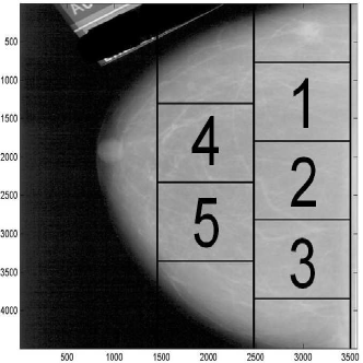
Figure 1: Five subimages of size $1024\times 1024$ are extracted from each breast image to capture tissues from the designated locations.

4.2 Estimation of $H$

For every subimage, the DWT using Haar and Symmlet 8-tap filters were performed to observe sensitivity in results under different wavelet bases. The analysis was repeated with four different sets of levels used for the regresion: 4 to 9, 5 to 9, 6 to 9, and 7 to 9. After each transform, OLS, AV, and TT estimation methods were used to compute the directional Hurst exponents, $H_{d}$, $H_{h}$, and $H_{v}$.

A nested ANOVA was performed to test if the Hurst estimates have significant differences based on the health condition of a patient,

$$H_{ijk}=\mu+\alpha_{i}+\beta_{j(i)}+\epsilon_{ijk},$$

where $i$ indicates the health status of a patient ($i$=1 for cancer, $i$=2 for normal), $j(i)$ indicates a patient nested in the status $i$, ($j(1)=1,\dots,45;j(2)=1,\dots,79$), and $\epsilon_{ijk}$ is an error term ($k=1,\dots,5$). Table 5 summarizes the results of the ANOVA analysis on diagonal Hurst exponents ($H_{d}$) obtained using Symmlet 8 tap filter and the TT method.

Table 5: ANOVA results on $H_{d}$ using Symmlet 8 and the TT method.

Source	Sum Sq.	d.f.	Mean Sq.	F	p-value
Status	0.330	1	0.330	10.741	0.001
Patients(Status)	3.750	122	0.031	7.574	$<$0.001
Error	2.013	496	0.004
Total	6.093	619

Note that 5 images are taken for each subject. This gives a total number of images $(45+79)\times 5=620.$ However, since the subjects had multiple images and were used as blocks within the disease status, the nested ANOVA was necessary to correctly analyze this data.

The ANOVA model used was also demonstrated to be appropriate by checking for the normality and independence of residuals. The $n=620$ residuals at each hierarchy $H_{d}$, $H_{h}$ and $H_{v}$ conformed to a battery of standard goodness-of-fit and independence tests. We were particulary focused on the deviations from the symmetry of residuals, given non-robustness of standard ANOVA to alternatives of asymmetry. To this end, the Lin-Mukholkar and Jarque-Bera tests were conducted and found not significant. At first glance the independence is a non-issue here, since the observations could be freely permuted in each of the disease classes. This, however, is not the case since the positions of subimages 1-5 are comparable within each mammogram. The Durbin-Watson test of independence against the order of residuals was found insignificant as well.

The $p$-values for disease factor from the ANOVA analysis were 0.001 for $H_{d}$ (Table 5), 0.003 for $H_{h}$, and 0.020 for $H_{v}$. Based on the ANOVA analysis, we conclude that a patient’s health condition is a significant factor that affects Hurst exponents in any of the three directions: diagonal, horizontal, and vertical. In the subsequent classification procedure based on ANOVA estimators of disease status, it is shown that these main effects are not only statistically significant, but also discriminatory.

4.3 Classification of Images

To classify mammogram images as cancerous or non-cancerous, the estimated $H_{d}$ and pair ($H_{d},H_{h}$) for each subject were taken using nested ANOVA. Operationally, this is $H_{ij,d}=\mu+\alpha_{i}+\beta_{j(i)}.$

Next, the subjects were classified by disease status using a logistic regression with four fold cross validation. The classification was repeated 300 times and the results were averaged over these 300 repetitions. A threshold of the logistic regression based on the maximum Youden index was chosen, which indicates the threshold (i.e., 0.6057) providing the maximum true positive and true negative accuracy.

Table 6: Results of classification by logistic regression using $H_{d}$ and $H_{d},H_{h}$

Predictors		$H_{d}$				$H_{d}$, $H_{h}$
Method		Total	Specificity	Sensitivity		Total	Specificity	Sensitivity
OLS		0.648	0.567	0.682		0.626	0.554	0.707
AV		0.652	0.511	0.733		0.640	0.502	0.747
TT		0.654	0.550	0.709		0.639	0.537	0.725

Table 6 summarizes the results of the classification based on $H_{d}$ and ($H_{d},\;H_{h}$), for each estimation method. The first column provides total classification accuracy, while the next two columns provide true positive and true negative rates. The best classification rates were achieved with the TT and AV estimators, where the classification error was around 35% for both methods. OLS was the worst performer, with 36% error.

Unlike the simulation cases where the monofractality of the signals were violated by design, and where the TT method was clearly favored, for mammograms the AV and TT methods performed comparably. This may be the consequence of the fact that individual $1024\times 1024$ subimages taken from the mammograms exhibited reasonable isotropy and monofractality, with wavelet coefficients being aproximately Gaussian.

Figure 2 shows a ROC curve of $H_{d}$ (obtained by TT) in differentiating between controls and cancer cases. The diagonal line represents a test with a sensitivity of 50% and a specificity of 50%. This shows the ROC curve lying significantly to the left of the diagonal, where the combination of sensitivity and specificity are highest. The area under the ROC curve, which is proportional to the diagnostic accuracy of the test, is 0.678.

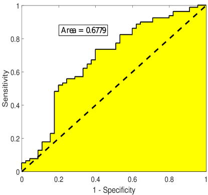
Figure 2: ROC curve for the logistic regression:$\mbox{logit}(p)=5.027-7.968\cdot H_{d}$.

5. Discussion & Conclusions

In this paper a novel wavelet-based Theil-type (TT) robust estimator of scaling was presented, with theoretically optimal weights for pairwise slopes that depend on harmonic average of sample sizes from the two multiresolution levels defining the pair. This estimator is free of distributional assumptions for the underlying regression, and robust with respect to possible outlier levels. An extensive simulational study demonstrated that the TT estimator was comparable, and in many scenarios superior, to the standardly used ordinary least squares (OLS) and Abry-Veitch (AV) estimators. This superiority is reflected in both less bias and smaller mean-squared error.

In the context of mammogram classification, the TT method was found to be comparable to AV and superior to OLS methods. This closeness of TT and AV could be explained by apparent relative spatial homogeneity and monofractality of the mammogram subimages used in the analysis.

For all three estimators considered, adding spectral indices from directional hierarchies other than the diagonal did not always improve the diagnostic performance. Index $H_{d}$ by itself was strongly discriminatory and the most parsimonious classifying summary. Furthermore, the results of classification using all three spectra ($H_{d},H_{h}$, and $H_{v}$) did not always perform better, on average, than that with only one or two spectral indices.

The diagnostic use of information contained in the background of images is often an ignored modality. It allows for the use of information from the entire image, rather than focusing primarily on irregular shapes, masses, or calcifications.

Recently, many studies have proposed fractal based modeling to describe and detect the pathological architecture of tumors. For example, the authors in Hermann et al., (2015) demonstrated breast cancer screening using fractal and stochastic geometric approaches such as random carpets, Quermass-interaction process, and complex-wavelet based self-similarity measures.

Although medical images exhibit high heterogeneity attributing to their multifractality, the use of the robust estimator proposed in this paper has proven that the monofractal self-similarity measure can be a promising classifier to differentiate malignant images from benign. As it is important to combine several instruments for cancer testing, this paper provides a quick and robust quantitative measure to strengthen existing mammogram classification procedures. Although the accuracy rates could be argued to be relatively low, even classifiers that are “slightly better than flipping a coin” can improve diagnostic accuracy when added to a battery of other independent testing modalities.

Finally, as future work, the authors plan to extend Ramírez-Cobo and Vidakovic, (2013), where the multifractal spectrum was used for diagnostic classification in a similar context. Some experiments in this direction were conducted in Ramírez-Cobo and Vidakovic, (2012), however, direct comparisons with the results in this paper were not possible because of different data sets used.

Acknowledgement.  The corresponding author thanks the projects MTM2015-65915 (Ministerio de Economía y Competitividad, Spain), P11-FQM-7603 and FQM-329 (Junta de Andalucía), all with EU ERD Funds. Brani Vidakovic was supported by NSF-DMS 1613258 award and the National Center for Advancing Translational Sciences of the National Institutes of Health under award UL1TR000454.

BIBLIOGRAPHY

APPENDIX A: Derivation of the weights of the TT approach

Let $d_{j}=d_{j{\mathbf{k}}}$ be an arbitrary (wrt $\mathbf{k}$) wavelet coefficient from the $j$th level of the decomposition of the $m$-dimensional fractional Brownian motion $B_{H}(\omega,\mathbf{t}),\mathbf{t}\in\mathbb{R}^{m}$,

$$d_{j}=\int_{\mathbb{R}^{m}}~{}B_{H}(\omega,\mathbf{t})\psi^{*}_{j\mathbf{k}}(\mathbf{t})d\mathbf{t},$$

for some fixed $\mathbf{k}=(k_{1},\dots,k_{m}).$ Here $\psi^{*}_{j\mathbf{k}}(\mathbf{t})=\prod_{i=1}^{m}\psi^{*}_{jk_{i}}(t_{i})$ where $\psi^{*}$ is either $\psi$ or $\phi$, but in the product there is at least one $\psi.$ It is well known that

$$d_{j}\stackrel{{\scriptstyle d}}{{=}}2^{-(H+m/2)j}~{}d_{0},$$

where $d_{0}$ is a coefficient from the level $j=0,$ and $\stackrel{{\scriptstyle d}}{{=}}$ means equality in distributions.

Coefficient $d_{j}$ is a random variable with

$$\mathbb{E\,}d_{j}=0\;~{}\text{and}\;~{}\mathbb{V}{\bf{ar\,}}d_{j}=\mathbb{E\,}d_{j}^{2}=2^{-(2H+m)j}~{}\sigma^{2},$$

where $\sigma^{2}=\mathbb{V}{\bf{ar\,}}d_{0}.$

The fBm $B_{H}(\omega,\mathbf{t})$ is a Gaussian $m$-dimensional field, thus

$$d_{j}\sim{\cal N}(0,2^{-(2H+m)j}\sigma^{2}).$$

The coefficients $d_{j}$ within the level $j$ are typically considered approximately independent. The covariance decays with the distance between the coefficients and the rate of decay depends on $H$ and $N$ - the number of vanishing moments for the wavelet $\psi.$ Flandrin, (1992) and Tewfik and Kim, (1992) showed that for $m=1$,

$$\mathbb{E\,}d_{jk_{1}}d_{jk_{2}}\leq C|k_{1}-k_{2}|^{2(H-N)},$$

where $C$ depends on $j.$ Although, for small $|k_{1}-k_{2}|$ this covariance may not be small, it decays to 0 as long as $N>H.$ To ensure short memory of $d_{jk},~{}k\in\mathbb{Z},$ the convergence of

$$\sum_{k}\mathbb{E\,}|d_{jk_{1}}d_{jk_{2}}|$$

is needed, for which it is required that $N>H+1/2.$

The rescaled “energy”

$$\frac{2^{(2H+m)j}}{\sigma^{2}}d_{j}^{2}\sim\chi^{2}_{1},$$

while, assuming the independence of $d_{jk}$’s,

$$\frac{2^{(2H+m)j}}{\sigma^{2}}\sum_{\mathbf{k}\in\mbox{\footnotesize$j$th level}}d_{j\mathbf{k}}^{2}=\frac{2^{(2H+2m)j}}{\sigma^{2}}~{}\overline{d_{j}^{2}},$$

has $\chi^{2}_{2^{mj}}$ distribution. Here, $\overline{d_{j}^{2}}$ is the average energy in $j$th level.

Thus,

$$\overline{d_{j}^{2}}\stackrel{{\scriptstyle d}}{{=}}2^{-(2H+2m)j}\sigma^{2}\chi^{2}_{2^{mj}}.$$

From this,

$$\mathbb{E\,}\overline{d_{j}^{2}}=\sigma^{2}2^{-(2H+2m)j}\mathbb{E\,}\chi^{2}_{2^{mj}}=2^{-(2H+m)j}\sigma^{2},$$

and

$$\mathbb{V}{\bf{ar\,}}\overline{d_{j}^{2}}=\sigma^{4}2^{-(4H+4m)j}\times 2\cdot 2^{mj}=2^{-4Hj-3mj+1}\sigma^{4}.$$

Recall that if $X$ has $\mathbb{E\,}X$ and $\mathbb{V}{\bf{ar\,}}X$ finite and $\varphi$ is a function with finite second derivative at $\mathbb{E\,}X$, then

$$\mathbb{E\,}\varphi(X)\approx\varphi(\mathbb{E\,}X)+\frac{1}{2}\varphi^{\prime\prime}(\mathbb{E\,}X)\cdot\mathbb{V}{\bf{ar\,}}X,$$

and

$$\mathbb{V}{\bf{ar\,}}\varphi(X)\approx(\varphi^{\prime}(\mathbb{E\,}X))^{2}\mathbb{V}{\bf{ar\,}}X.$$

When $\varphi$ is logarithm for base 2, then

$$\mathbb{E\,}\log_{2}\overline{d_{j}^{2}} = \log_{2}\mathbb{E\,}\overline{d_{j}^{2}}+\frac{1}{2\log 2}\left(-\frac{\mathbb{V}{\bf{ar\,}}\overline{d_{j}^{2}}}{\left(\mathbb{E\,}\overline{d_{j}^{2}}\right)^{2}}\right)$$

$$= \log_{2}\left(2^{-(2H+m)j}\sigma^{2}\right)-\frac{1}{2\log 2}2^{-mj+1}$$

$$= -(2H+m)j-\frac{1}{2^{mj}\log 2}+\log_{2}\sigma^{2}.$$

Note that $-\frac{1}{2^{mj}\log 2}$ is the Abry-Veitch bias term, and it is free of $H$ and $\sigma^{2}.$ This bias is a second order approximation. Veitch and Abry show that the exact bias involves digamma function $\Psi$, and in this context is

$$\frac{\Psi(2^{mj-1})}{\log 2}-\log\left(2^{mj-1}\right).$$

Also,

$$\mathbb{V}{\bf{ar\,}}\log_{2}\overline{d_{j}^{2}} = \left(\frac{1}{\sigma^{2}~{}2^{-(2H+m)j}~{}\log 2}\right)^{2}$$

$$~{}~{}~{}\times\sigma^{4}\cdot 2^{-4Hj-3mj+1}$$

$$= \frac{2}{2^{mj}(\log 2)^{2}}.$$

Finally,

$$\mathbb{V}{\bf{ar\,}}\left(\frac{\log_{2}\overline{d_{j}^{2}}-\log_{2}\overline{d_{i}^{2}}}{j-i}\right)=\frac{2}{(\log 2)^{2}}\cdot\frac{1/2^{mj}+1/2^{mi}}{(j-i)^{2}}.$$

Since weights $w_{ij}$ are inverse-proportional to the variance, then

$$w_{ij}\propto(i-j)^{2}\times HA(2^{mi},2^{mj}),$$

where $HA$ is the harmonic average.

BIBLIOGRAPHY

- Abry, (2003) Abry, P. (2003). Scaling and wavelets: an introductory walk, volume 621 of Lecture Notes in Physics, pages 34–60.
- Abry et al., (2000) Abry, P., Flandrin, P., Taqqu, M., and Veitch, D. (2000). Wavelets for the analysis, estimation, and synthesis of scaling data. In Park, K. and Willinger, W., editors, Self-Similar Network Traffic and Performance Evaluation. Wiley.
- Abry et al., (2001) Abry, P., Flandrin, P., Taqqu, M., and Veitch, D. (2001). Self-similarity and long-range dependence through the wavelet lens. In Doukhan, P., Oppenheim, G., and Taqqu, M., editors, Long Range Dependence: Theory and Applications. Birkhauser.
- Altekruse et al., (2010) Altekruse, S., Kosary, C., Krapcho, M., Neyman, N., Aminou, R., and Waldron, W. (2010). Seer cancer statistics review, 1975-2007.
- Audit et al., (2002) Audit, B., Bacry, E., Muzy, J. F., and Arneodo, A. (2002). Wavelet-based estimators of scaling behavior. IEEE Transactions on Information Theory, 48(11):2938–2954.
- Beran, (1994) Beran, J. (1994). Statistics for Long-memory Processes. Chapman Hall, New York.
- Birkes and Dodge, (1993) Birkes, D. and Dodge, Y. (1993). Alternative Methods of Regression. Wiley, New York, NY.
- Coeurjolly, (2000) Coeurjolly, J.-F. (2000). Simulation and identification of the fractional brownian motion: a bibliographical and comparative study. Journal of Statistical Software, 5(i07):1–53.
- Craigmile and Percival, (2005) Craigmile, P. F. and Percival, D. B. (2005). Asymptotic decorrelation of between-scale wavelet coefficients. IEEE Transactions on Information Theory, 51(3):1039–1048.
- Daubechies, (1992) Daubechies, I. (1992). Ten Lectures on Wavelets. CBMS-NSF Regional Conference Series in Applied Mathematics. Society for Industrial and Applied Mathematics, Philadelphia, PA.
- El-Naqa et al., (2002) El-Naqa, I., Yang, Y., Wernick, M., Galatsanos, N., and Nishikawa, R. (2002). A support vector machine approach for detection of microcalcifications. IEEE Transactions on Medical Imaging, 21(12):1552–1563.
- Engel Jr et al., (2009) Engel Jr, J., Bragin, A., Staba, R., and Mody, I. (2009). High-frequency oscillations: what is normal and what is not? Epilepsia, 50(4):598–604.
- Flandrin, (1992) Flandrin, P. (1992). Wavelet analysis and synthesis of fractional brownian motion. IEEE Transactions on Information Theory, 38(2):910–917.
- Franzke et al., (2005) Franzke, C., Graves, T., Watkins, N., Gramacy, R., and Hughes, C. (2005). Robustness of estimators of long-range dependence and self-similarity under non-gaussianity. Philosophical Transactions of the Royal Society A, 370:1250–1267.
- Gregoriou et al., (2009) Gregoriou, G., Gotts, S., Zhou, H., and Desimone, R. (2009). High-frequency, long-range coupling between prefrontal and visual cortex during attention. Science, 324(5931):1207–1210.
- Hamilton et al., (2011) Hamilton, E. K., Jeon, S., Ramírez Cobo, P., Lee, K., and Vidakovic, B. (2011). Diagnostic classification of digital mammograms by wavelet-based spectral tools: A comparative study. In Proceedings of IEEE International Conference on Bioinformatics and Biomedicine, Atlanta, GA, November 12-15, pages 384–389, Atlanta, GA.
- Heath et al., (2000) Heath, M., Bowyer, K., Kopans, D., Moore, R., and Kegelmeyer, P. (2000). The Digital Database for Screening Mammography, pages 212–218. 5th International Workshop on Digital Mammography, Toronto, Canada. Medical Physics Publishing, Madison, WI.
- Hermann et al., (2015) Hermann, P., Mrkvicka, T., Mattfeldt, T., Minarova, M., Helisova, K., Nicolis, O., Wartner, F., and Stehlík, M. (2015). Fractal and stochastic geometry inference for breast cancer: a case study with random fractal models and quermass-interaction process. Statistics in Medicine, 34:2636–2661.
- Jaeckel, (1972) Jaeckel, L. (1972). Estimating regression coefficients by minimizing the dispersion of residuals. Annals of Mathematical Statistics, 43:1449–1458.
- Jeon et al., (2014) Jeon, S., Nicolis, O., and Vidakovic, B. (2014). Mammogram diagnostics via 2-d complex wavelet-based self-similarity measures. São Paulo Journal of Mathematical Sciences, 8(2):256–284.
- Katul et al., (2001) Katul, G., Vidakovic, B., and Albertson, J. (2001). Estimating global and local scaling exponents in turbulent flows using wavelet transformations. Physics of Fluids, 13(1):241–250.
- Kestener et al., (2001) Kestener, P., Lina, J., Saint-Jean, P., and Arneodo, A. (2001). Wavelet-based multifractal formalism to assist in diagnosis in digitized mammograms. Image Analysis and Stereology, 20(3):169–175.
- Kiran Bala and Audithan, (2014) Kiran Bala, B. and Audithan, S. (2014). Wavelet and curvelet analysis for the classification of microcalcification using mammogram images. Second International Conference of Current Trends in Engineering and Technology, ICCTET14 (IEEE), pages 517–521.
- Kourou et al., (2015) Kourou, K., Exarchos, T. P., Exarchos, K. P., Karamouzis, M. V., and Fotiadis, D. I. (2015). Machine learning applications in cancer prognosis and prediction. Computational and Structural Biotechnology Journal, (13):8–17.
- Lévy, (1948) Lévy, P. (1948). Processus Stochastiques et Mouvement Brownien. Gauthier-Villars, Paris, France.
- Lutton et al., (2007) Lutton, E., Véhel, J. L., Herbin, E., Cayla, E., Louchet, J., Rocchisani, J.-M., Olague, G., Perez-Castro, C., Trujillo, L., Barriére, O., Aichour, M., and Guével, R. L. (2007). Analysis of irregular processes, images and signal, applications in biology and medicine.
- Mallat, (1998) Mallat, S. (1998). A Wavelet Tour of Signal Processing. Academic Press, San Diego, CA.
- Netsch and Peitgen, (1999) Netsch, T. and Peitgen, H. (1999). Scale-space signatures for the detection of clustered microcalcifications in digital mammograms. IEEE Transactions on Medical Imaging, 18(9):774–786.
- Nicolis et al., (2011) Nicolis, O., Ramírez-Cobo, P., and Vidakovic, B. (2011). 2D wavelet-based spectra with applications. Computational Statistics & Data Analysis, 55(1):738–751.
- Park and Park, (2009) Park, J. and Park, C. (2009). Robust estimation of the Hurst parameter and selection of an onset scaling. Statistica Sinica, 19(4):1531–1555.
- Park and Willinger, (2000) Park, K. and Willinger, W. (2000). Self-Similar Network Traffic and Performance Evaluation. Wiley, New York, NY.
- Ramírez-Cobo and Vidakovic, (2012) Ramírez-Cobo, P. and Vidakovic, B. (2012). A note on robust multifractal spectra. Technical report, ISyE, Georgia Institute of Technology.
- Ramírez-Cobo and Vidakovic, (2013) Ramírez-Cobo, P. and Vidakovic, B. (2013). A 2D wavelet-based multiscale approach with applications to the analysis of digital mammograms. Computational Statistics & Data Analysis, 58(1):71–81.
- Reed et al., (1995) Reed, I. S., Lee, P. C., and Truong, T. K. (1995). Spectral representation of fractional brownian motion in N dimensions and its properties. IEEE Transactions on Information Theory, 41(5):1439–1451.
- Roberts et al., (2017) Roberts, T., Newell, M., Auffermann, W., and Vidakovic, B. (2017). Wavelet-based scaling indices for breast cancer diagnostics. Statistics in Medicine, 36(12):1989–2000.
- Shen et al., (2007) Shen, H., Zhu, Z., and Lee, T. (2007). Robust estimation of the self-similarity parameter in network traffic using wavelet transform. Signal Processing, 87(9):2111–2124.
- Sheng et al., (2011) Sheng, H., Chen, Y., and Qiu, T. (2011). On the robustness of Hurst estimators. IET Signal Processing, 5(2):209–225.
- Sievers, (1978) Sievers, G. (1978). Weighted rank statistics for simple linear regression. Journal of the American Statistical Association, 73:628–631.
- Soltani et al., (2004) Soltani, S., Simard, P., and Boichu, D. (2004). Estimation of the self-similarity parameter using the wavelet transform. Signal Processing, 84(1):117–123.
- Tewfik and Kim, (1992) Tewfik, A. and Kim, M. (1992). Correlation structure of the discrete wavelet coefficients of fractional Brownian motion. IEEE Transactions on Information Theory, 38:904–909.
- Theil, (1950) Theil, H. (1950). A rank-invariant method of linear and polynomial regression analysis. Indagationes Mathematicae, 12:85–91.
- Veitch and Abry, (1999) Veitch, D. and Abry, P. (1999). A wavelet-based joint estimator of the parameters of long-range dependence. IEEE Transactions on Information Theory, 45(3):878–897.
- Wang and Karayiannis, (1998) Wang, T. C. and Karayiannis, N. B. (1998). Detection of microcalcifications in digital mammograms using wavelets. IEEE Transactions on Medical Imaging, 17(4):498–509.
- Wilcox, (2001) Wilcox, R. R. (2001). Theil-Sen estimator. In Fundamentals of Modern Statistical Methods: Substantially Improving Power and Accuracy, pages 207–210. Springer-Verlag.
- Wood and Chan, (1994) Wood, A. T. A. and Chan, G. (1994). Simulation of stationary gaussian processes in . Journal of Computational and Graphical Statistics, 3(4):409–432.
- Woods et al., (2016) Woods, T., Preeprem, T., Lee, K., Chang, W., and Vidakovic, B. (2016). Characterizing exons and introns by regularity of nucleotide strings. Biology Direct, 11(6):1–17.
- Zhou, (1996) Zhou, B. (1996). High-frequency data and volatility in foreign-exchange rates. Journal of Business Economic Statistics, 14(1):45–52.