Sparse-view Cone Beam CT Reconstruction using Data-consistent Supervised and Adversarial Learning from Scarce Training Data

Abstract

Reconstruction of CT images from a limited set of projections through an object is important in several applications ranging from medical imaging to industrial settings. As the number of available projections decreases, traditional reconstruction techniques such as the FDK algorithm and model-based iterative reconstruction methods perform poorly. Recently, data-driven methods such as deep learning-based reconstruction have garnered a lot of attention in applications because they yield better performance when enough training data is available. However, even these methods have their limitations when there is a scarcity of available training data. This work focuses on image reconstruction in such settings, i.e., when both the number of available CT projections and the training data is extremely limited. We adopt a sequential reconstruction approach over several stages using an adversarially trained shallow network for ‘destreaking’ followed by a data-consistency update in each stage. To deal with the challenge of limited data, we use image subvolumes to train our method, and patch aggregation during testing. To deal with the computational challenge of learning on 3D datasets for 3D reconstruction, we use a hybrid 3D-to-2D mapping network for the ‘destreaking’ part. Comparisons to other methods over several test examples indicate that the proposed method has much potential, when both the number of projections and available training data are highly limited.

I Introduction

Computed Tomography (CT) is an important imaging modality across applications in medicine, industry, science and security. In this work, we develop an iterative machine learning-based approach for 3D cone beam CT reconstruction from very limited measurements or projections, and using limited training data. In the following, we first review some background in limited-view CT reconstruction before highlighting the contributions of this work.

I-A Background

Cone Beam CT (CBCT) is a CT-based technique that allows for three-dimensional imaging of an object using X-rays diverging from a source. In CBCT, an entire 3D image volume is reconstructed from a set of 2D projections through the corresponding object. These projections/measurements are obtained at different angles or ‘views’ around the object, and are collectively dubbed a sinogram. There are several approaches for the inverse problem of obtaining an image from these measurements. A classical method for this task is the analytical Feldkamp-Davis-Kress (FDK) algorithm [1]. More sophisticated methods for 2D or 3D reconstruction involve model-based reconstruction using iterative algorithms [2, 3, 4], and data-driven algorithms [5, 6].

Model-based image reconstruction (MBIR) or statistical image reconstruction (SIR) methods exploit sophisticated models for the physics of the imaging system and models for sensor and noise statistics as well as for the underlying object. These methods iteratively optimize for the underlying image based on the system forward model, measurement statistical model, and assumed prior for the underlying object [7, 8, 9, 10]. In particular, penalized weighted least squares (PWLS) approaches have been popular for CT image reconstruction that optimize a combination of a statistically weighted quadratic data-fidelity term (capturing the forward and noise model) and a regularizer penalty that captures prior information of the object [11]. MBIR methods have often used simple regularizers [12] such as edge-preserving regularization involving nonquadratic functions of differences between neighboring pixels [13] (implying image gradients may be sparse) or other improved regularizers [14, 15, 16, 17].

Within the class of data-driven approaches, dictionary learning [12] and deep learning based methods for reconstruction have gained popularity in recent years due to their demonstrated effectiveness in removing artifacts from images in a variety of modalities, great flexibility and the availability of curated datasets for training [18, 19, 20].

However, in several applications, acquiring many projections or ‘views’ through the object may be undesirable or impossible. This constraint may be to reduce exposure to radiation in medical imaging applications, or due to only pre-set limited or sparse views being possible in industrial or security applications. Moreover, in dynamic imaging applications, where the object is changing while being imaged, we would also be limited to fewer views per temporal state, to prevent blurring. While total variation (TV)-based MBIR methods have been extensively applied to such sparse-view and sparse angle reconstruction problems [21, 22, 23, 24, 25, 26], other model-based CT reconstruction algorithms rely upon learned prior-based regularizers [27, 28, 29]. These methods often require many iterations to converge, leading to large runtimes, and also require careful selection of regularization parameters to obtain reasonable image quality trade-offs.

Deep learning-based algorithms have also found considerable use in many problems ranging from artifact correctionto combination with model-based reconstruction [30, 31, 32, 33]. Deep learning approaches could be supervised or unsupervised or mixed [34, 35] and include image-domain (denoising) methods, sensor-domain methods, AUTOMAP, as well as hybrid-domain methods (cf. reviews in [12, 36]). Hybrid-domain methods are gaining increasing interest and enforce data consistency (i.e., the reconstruction should be consistent with the measurement model) during training and reconstruction to improve stability and performance. Deep learning methods often require large training data sets and long training times to work well. They may also struggle to generalize to data with novel features or that are obtained with different experimental settings.

When reconstructing 3D objects from extremely limited tomographic views or projections, many of the aforementioned approaches fail. The FDK algorithm yields reconstructions that are severely ridden with streak artifacts. While conventional iterative methods perform better, the quality of reconstructions leave a lot to be desired, and there is often poor bias-variance trade-offs. Deep learning-based approaches have the potential to perform better in this scenario, but still perform poorly when there is a scarcity of available data for training, such as in national security applications where experimental data is limited and accurate simulations are expensive [37]. While there are approaches that reconstruct from very limited projections, they either do not target 3D CBCT imaging [19, 25, 38, 39], or rely upon many paired training image volumes [40, 18, 20].

I-B Contributions

This paper focuses on developing a method that can provide quality reconstructions from extremely limited projections even with very extremely limited training data. The proposed reconstruction approach works across multiple stages, similar to an unrolled-loop algorithm [12], where each stage consists of a shallow CNN block trained using a combined supervised and adversarial loss, followed by a data-consistency block. The adversarial component of our loss yields destreaked images that have more realistic texture. To mitigate the challenge of reduced training data, we reduce the scope of our learning to patches or image sub-volumes. This approach allows us to provide several training examples from even a single training image. Destreaked patches are aggregated before data-consistency is applied to the whole volume. Furthermore, we prime our method using an edge-preserving regularized reconstruction as input.

We compare our methods to a variety of techniques including the FDK algorithm, edge-preserving regularized reconstruction, and deep CNN-based reconstruction without data-consistency. Simulation results suggest that the proposed method provides much better image quality than previous techniques with extremely limited (four or eight) views of 3D objects.

I-C Organization

The rest of this paper is organized as follows. Section II describes the proposed approach in detail. Section III explains our choices for various algorithm parameters as well as our experimental setup. Section IV presents the results of our comparisons to other algorithms as well as other experiments that offer insights into the process of our reconstruction. Section V elaborates upon these observations. Finally, Section VI states our conclusions and offers some avenues for future research.

II Algorithm & Problem Setup

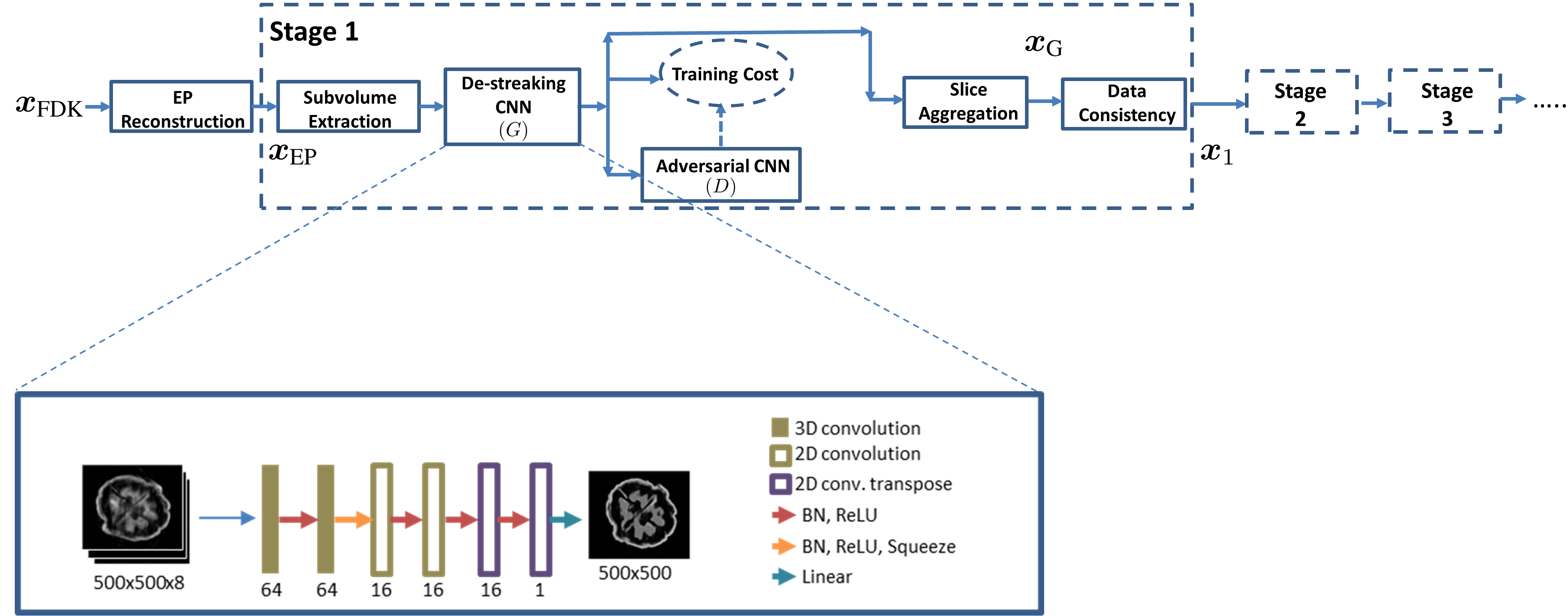
Figure 1: Flow diagram depicting the overall pipeline of our algorithm, where $\bm{x}_{\text{FDK}}$ is the FDK reconstruction, $\bm{x}_{\text{EP}}$ is an edge-preserving regularized reconstruction, $\bm{x}_{\text{G}}$ is the generator’s output after slice aggregation, and $\bm{x}_{1}$ is the output of the first stage.

Our proposed method for CBCT reconstruction focuses on addressing two primary challenges: a very limited number of available views, and limited number of available training objects. We address the former through a combination of three aspects: (1) using an edge-preserving regularized reconstruction [4] to initialize our iterative-type algorithm; (2) including an adversarial component to the training loss function for our learned destreaking networks (similar to generative adversarial networks or GANs); and (3) including data-consistency blocks that reinforce acquired measurements in the destreaked 3D reconstruction.

The problem of scarce training data is addressed primarily by two approaches. First, we split an entire image volume into patches in the form of overlapping subvolumes. Essentially, this step localizes the scope of CNN-based destreaking to a comparatively smaller neighborhood, while allowing us to generate many training examples from a single image volume. Second, we use a shallow destreaking CNN to avoid overfitting to the training data. To reduce computation time associated with multiple 3D convolutions and subsequent patch aggregation, the CNN is designed to map 3D subvolumes to 2D slices [41]. This approach enables using 3D contextual information for the destreaking task, while removing the need for patch averaging (of overlapping 3D patches) and associated artifacts during aggregation.

Many learning-based reconstruction approaches in applications like MRI work through end-to-end training, whereas such approaches are less practicle in CT due to the complexity of the system matrix. Thus, our developed algorithm operates as a multi-stage greedy approach similar to works like [42, 43]. Each stage is composed of a CNN that maps each 3D subvolume with streaking artifacts to a clean 2D slice corresponding to the slice at the centre of the subvolume. Because the objects considered here have finite support, we treat the slices at the edge of the volume in the direction of aggregation are being empty, and set them to zero. One could use other boundary conditions for long objects [44]. Once an entire image volume has been aggregated from individual clean slices, this volume is passed through a data-consistency update to reinforce acquired measurements and reduce any ‘hallucinations’ introduced by the network. This output subvolume is then provided as input to the next stage. Fig. 1 depicts the process that is akin to algorithm unrolling [45]. As mentioned earlier, to reduce noise and streaks, the input to the first stage of our method is an edge-preserving regularized (iteratively obtained) reconstruction, using the regularizer in [4] and the algorithm in [46], which in turn is initialized with an FDK reconstruction for faster convergence.

We train the CNN parameters separately for each stage. The training loss for the destreaking CNN in each stage consists of a weighted combination of a masked mean squared error term calculated over a region of interest using the ground truth training image slices, and an adversarial input from another CNN that acts as a discriminator for the output of the destreaking CNN (also specific to the stage). Adversarial training often is posed as a min-max optimization problem [47], but the practical implementation involves alternating between updating generator (destreaking) network $G$ parameters $\phi^{k}$ and discriminator network $D$ parameters $\theta^{k}$, with more frequent updates of the generator parameters. Our approach to updating the generator weights for the $k$th stage is mathematically expressed as:

$$\begin{split}\hat{\theta}^{k}=\arg\min_{\theta}&\ {-\lambda}\,\mathbb{E}\big{[}D_{\phi^{k}}(G_{\theta}(\mathcal{P}_{3}\bm{x}_{k-1}))\big{]}\\ &+\mathbb{E}\big{[}\|\mathcal{P}_{3}^{2,\text{mid}}\bm{x}_{\text{GT}}-G_{\theta}(\mathcal{P}_{3}\bm{x}_{k-1})\|_{2}^{2}\big{]},\end{split}$$ (1)

where $\bm{x}_{k-1}$ is the output of the $(k-1)$th stage of our algorithm, $\bm{x}_{0}$ is set to be $\bm{x}_{\text{EP}}$ (the edge-preserving regularized reconstruction), $\bm{x}_{\text{GT}}$ is the ground truth, $\lambda$ is a regularization parameter that varies as the weights of $G^{k}$ are updated (see Section III-B), $\mathcal{P}_{3}$ is a 3D patch or subvolume extraction operator, and $\mathcal{P}_{3}^{2,\text{mid}}$ is an operator that extracts the 2D central slice from an image subvolume, where the position of the subvolume is determined by $\mathcal{P}_{3}$. We restricted the reconstructions to a region in the image volume containing the object of interest. The expectation $\mathbb{E}$ is taken over the set of training examples.

Our approach to updating the the discriminator network parameters is likewise given as:

$$\begin{split}\hat{\phi}^{k}=\arg\min_{\phi}~{}&\mathbb{E}\big{[}\big{(}D_{\phi}(G_{\theta^{k}}(\mathcal{P}_{3}\bm{x}_{k-1}))-0\big{)}^{2}\big{]}\\ &+\mathbb{E}\big{[}\big{(}D_{\phi}(\mathcal{P}_{3}^{2,\text{mid}}\bm{x}_{\text{GT}})-1\big{)}^{2}\big{]}.\end{split}$$ (2)

The data-consistency update involves seeking an image that is consistent with the acquired measurements while still being ‘close’ to the slice-aggregated destreaked image. The optimization problem for this step is framed as:

$$\bm{x}_{k}=\underset{\bm{x}}{\textnormal{arg min}}\|\bm{A}\bm{x}-\bm{y}\|_{2}^{2}+\beta\|\bm{x}-\bm{x}_{k,\text{G}}\|_{2}^{2},$$ (3)

where $\bm{A}$ is the CBCT system matrix, implemented with the separable-footprint projector [48], $\bm{y}$ denotes the projections or acquired measurements, $\beta>0$ is a regularization parameter, and $\bm{x}_{k,\text{G}}$ is the output of the generator after slice aggregation at the $k$th stage. We used an ordinary least-squares (LS) data-fit term rather than a weighted LS (WLS) term because the focus here is on sparse views rather than low-dose imaging, but the method generalizes directly to the WLS case. We used 50 conjugate gradient (CG) iterations to minimize (3).

III Methods

III-A Dataset and Experimental Settings

To train and test our method, we used the publicly available 3D walnut CT dataset [49]. To study the ability to learn from very limited data, we used a single walnut for training our method, and tested our algorithm on 5 different walnuts. Furthermore, extremely limited data with 8 or 4 views/projections through the walnuts were used in training and testing the network. Separate networks were trained for reconstructing image volumes from 4 and 8 views, respectively. These CBCT views were generated using the MIRT [50] package, and were equally spaced over 360 degrees. The distance from source to detector was set to be 20 cm, and the distance from the object to the detector was 4.08 cm, and each projection view was $150\times 150$ pixels of size $\approx 0.4$ mm square. Because the CBCT system simulated here has a small cone angle (almost parallel beam), 8 views over 360^∘ probably has only a bit more information than 4 views over $180^{\circ}$. The image volume for each walnut was $501\times 501\times 501$. The dimensions of each voxel were approx. $0.12\times 0.12\times 0.12$ mm³.

III-B Hyperparameters and Network Architectures

The subvolume size for our scheme was chosen to be $500\times 500\times 8$. The parameter $\beta$ was chosen to be 1, and $\lambda$ was changed dynamically as the network weights were updated according to $10^{\lfloor\log(r)\rfloor}$, where $r=\mathbb{E}\big{[}\|\mathcal{P}_{3}^{2,\text{mid}}\bm{x}_{\text{GT}}-G_{\theta}(\mathcal{P}_{3}\bm{x}_{k-1})\|_{2}^{2}\big{]}$. This was done to maintain balance between the $\ell_{2}$ and adversarial loss components during generator training. The number of stages in our method was set to 4, and the networks in each stage were trained for 40 epochs. The weights for the discriminator were updated once for every 10 times the weights of the destreaking CNN were updated.

Fig. 1 depicts the generator architecture we used. The kernel size for 3D convolutions was ($3\times 3\times 3$), and ($3\times 3$) for the 2D convolutions. The discriminator was akin to a classifier with two convolutional layers and with 8 filters in each convolutional layer with ($3\times 3$) kernel size with stride 1 followed by fully connected layers with (1152,8,8) nodes respectively, with a sigmoid activation at the final output to constrain the output to be between 0 and 1. The batch size during training the destreaking CNNs was 6. Training the destreaking CNN in each stage of our algorithm took approx. 10 hours on 3 NVIDIA Quadro RTX 5000 GPUs, while at test time, each walnut volume required 7 minutes to reconstruct with a batch size of 3 on two of the same GPUs. The data consistency update required an additional 3 minutes on a workstation with Intel(R) Xeon(R) Silver 4214 CPU @ 2.20GHz with 48 cores.

III-C Compared Methods

To assess the performance of our method, we used 4 stages of our proposed algorithm to compromise between image quality and runtime. We compared the output for all 5 test walnuts to the conventional FDK reconstruction, an edge-preserving regularized (MBIR) reconstruction [4], as well as the slice-aggregated output from a single stage of our destreaking CNN without data consistency.

III-D Performance Metrics

We primarily used the normalized mean absolute error (NMAE) as a metric for evaluating the performance of various methods. The error is evaluated over the voxels within the region-of-interest (ROI) of a three-dimensional mask obtained by dilating a ground truth segmentation of the walnut being reconstructed. The masked region includes all voxels within the shell of the walnut. The NMAE normalization used the mean intensity of the ground truth voxels within this mask. Essentially, $E_{\text{NMAE}}(x_{GT},x_{O},\mathscr{M})=\|\mathscr{M}\odot(x_{GT}-x_{O})\|_{1}/\|\mathscr{M}\odot x_{GT}\|_{1}$, where $x_{GT}$ is the ground truth image volume, $x_{O}$ is the reconstruction whose quality is being evaluated, and $\mathscr{M}$ is a binary mask specific to the test walnut, which excludes any pixel not within the a dilation of the outer boundary of the walnut. These are obtained by a histogram-based thresholding of the corresponding ground truth volumes for the test walnuts.

Another metric that is used for comparison in our work is the normalized high-frequency error norm or NHFEN [51]. We computed the HFEN for every slice of the reconstructed walnut as the $\ell_{2}$ norm of the difference of masked edges (obtained through a high-pass filtering) between the input and reference images. The masking is done similarly as described earlier. A Laplacian of Gaussian (LoG) filter was used as the edge detector. The kernel size was set to $15\times 15$, with a standard deviation of 1.5 pixels. The normalization was performed over the high frequency components of the ground truth image over the masked ROI. Mathematically, this metric is calculated as $E_{\text{NHFEN}}(x_{GT},x_{O},\mathscr{M})=\frac{1}{N}\sum_{i}\|\mathscr{H}(\mathscr{M}[:,:,i]\odot x_{GT}[:,:,i])-(\mathscr{H}(\mathscr{M}[:,:,i]\odot x_{O}[:,:,i])\|_{2}/\|\mathscr{H}(\mathscr{M}[:,:,i]\odot x_{GT}[:,:,i])\|_{2}$, where $\mathscr{H}$ denotes the LoG filter described earlier, $i$ indexes the slices of the image volume in the $z$ direction, where $N$ is the total number of slices in that direction, and the other symbols have their usual meaning, as described previously. An advantage of using such normalized metrics is that it allows for the evaluation of the reconstruction quality only in areas of interest in the volume, disregarding the effect of empty spaces around it.

IV Results

Table I compares the reconstruction performance of various methods (including our own) described in the previous sections. The proposed approach substantially improves the NMAE and NHFEN compared to the reference methods for both 8 and 4 acquired projections. As expected, the quality of reconstructions using 4 acquired projections was worse than when 8 projections were acquired for reconstruction.

8 views
Walnut #	FDK recon.		EP recon.		CNN destreaking		Proposed
	NMAE	NHFEN	NMAE	NHFEN	NMAE	NHFEN	NMAE	NHFEN
1	0.77	0.90	0.45	0.58	0.40	0.59	0.26	0.54
2	0.77	0.88	0.45	0.57	0.38	0.58	0.25	0.53
3	0.79	0.90	0.49	0.61	0.42	0.62	0.30	0.58
4	0.79	0.96	0.45	0.62	0.39	0.62	0.27	0.58
5	0.82	0.98	0.48	0.65	0.41	0.66	0.27	0.61
4 views
Walnut #	FDK recon.		EP recon.		CNN destreaking		Proposed
	NMAE	NHFEN	NMAE	NHFEN	NMAE	NHFEN	NMAE	NHFEN
1	1.08	1.11	0.62	0.61	0.61	0.61	0.44	0.60
2	1.23	1.18	0.65	0.60	0.63	0.60	0.45	0.60
3	1.22	1.15	0.67	0.64	0.66	0.64	0.48	0.64
4	1.22	1.22	0.68	0.64	0.67	0.65	0.46	0.65
5	1.23	1.27	0.65	0.68	0.65	0.68	0.46	0.68

TABLE I: Comparison of the performance of our proposed method against FDK reconstruction, edge-preserving (EP) regularized reconstruction, a single stage of CNN-based destreaking without data-consistency (using the same architecture as in our method) and our proposed multistage reconstruction algorithm for 8 (top) and 4 (bottom) acquired projections. The metrics used for performance are the normalized mean absolute error (NMAE) and the normalized high-frequency error norm (NHFEN).

Fig. 2 gives an example reconstruction for 8 views (walnut 1 in Table I), showing central slices through the walnut in all three orientations (sagittal, coronal and transverse). The proposed algorithm provides significantly higher quality reconstructions than the other methods. This is particularly evident in the extent to which our algorithm is able to restore the finer features of the walnuts, and has fewer artifacts.

Ground Truth Test Volume	Ground Truth Training Volume
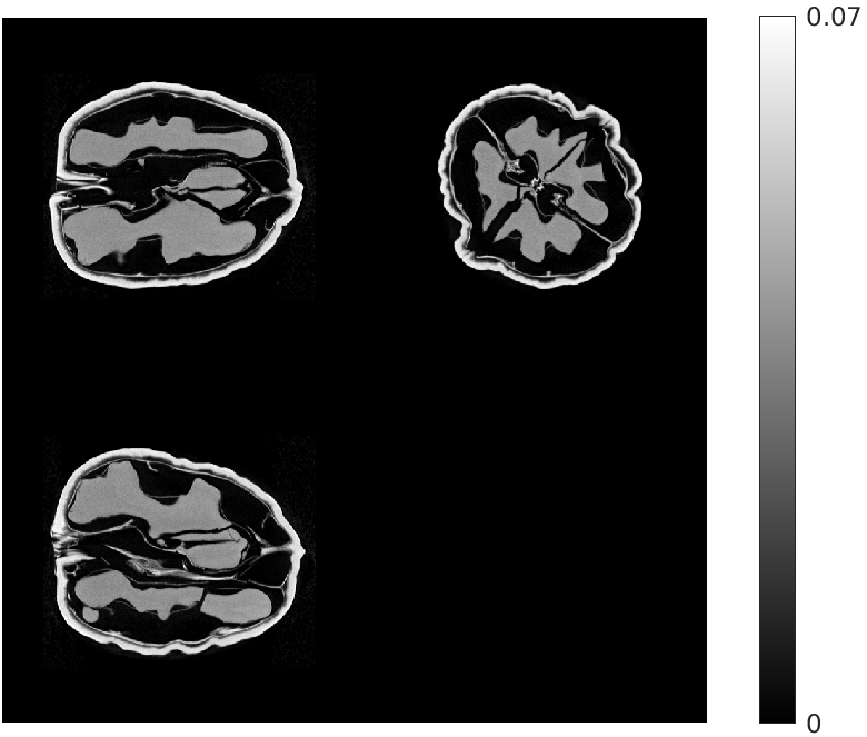
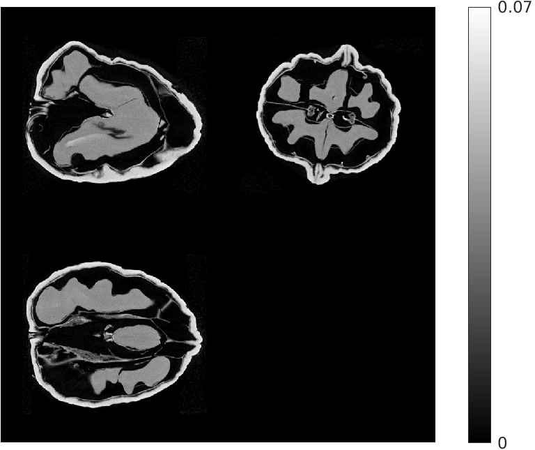
(a) (NMAE)	(b) (n/a)
FDK	EP Regularized Recon.
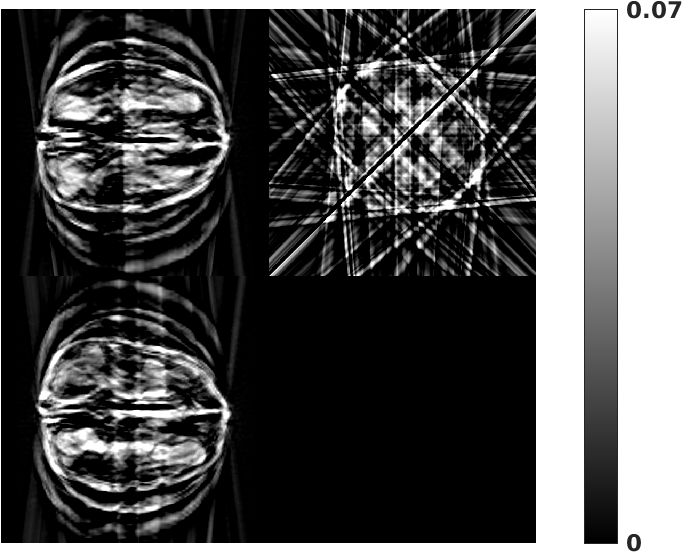
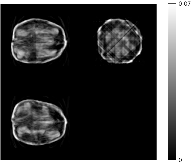
(c) (0.77)	(d) (0.45)
Destreaking CNN	Proposed
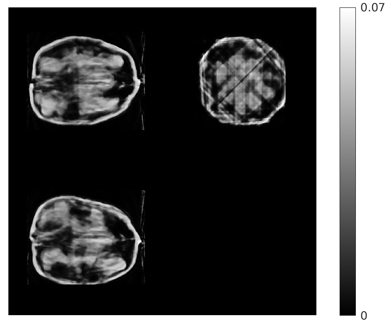
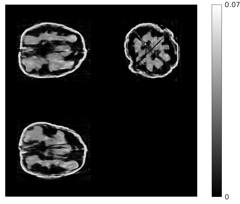
(e) (0.40)	(f) (0.26)

Figure 2: Comparison of the quality of reconstruction of our proposed algorithm (f) for walnut 1 (8 views) in Table I to various reference methods. Each subfigure depicts slices through the center of the walnut volume in the sagittal, coronal and transverse orientations. The normalized mean absolute errors have also been shown underneath each subfigure. The central slices corresponding to the ground truth training walnut volume have also been shown in (b).

Fig. 3 compares the reconstructions from 4 views. The quality of the reconstruction is poorer compared to that using 8 views, though the proposed approach still visibly outperforms the other methods.

Ground Truth Test Volume
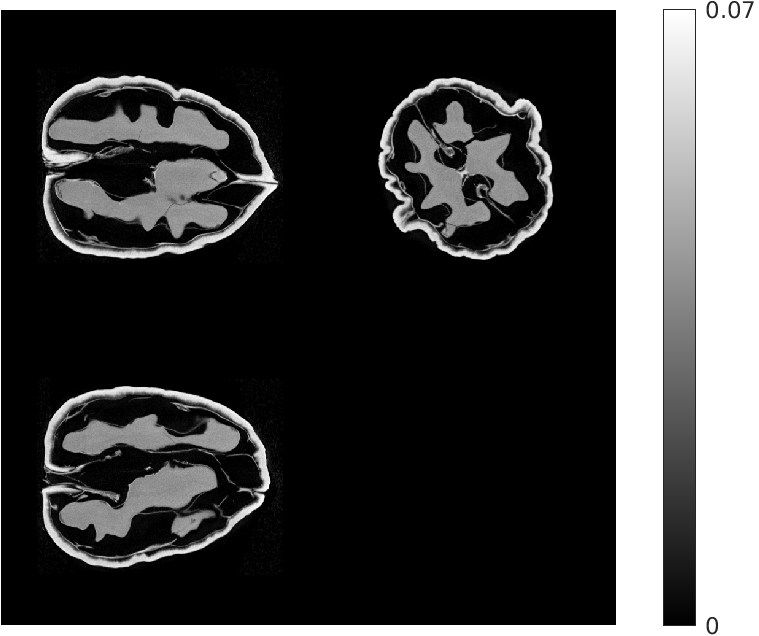
(a) (NMAE)
FDK	EP Regularized Recon.
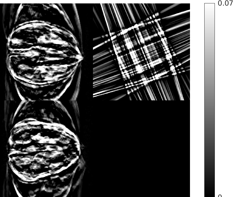
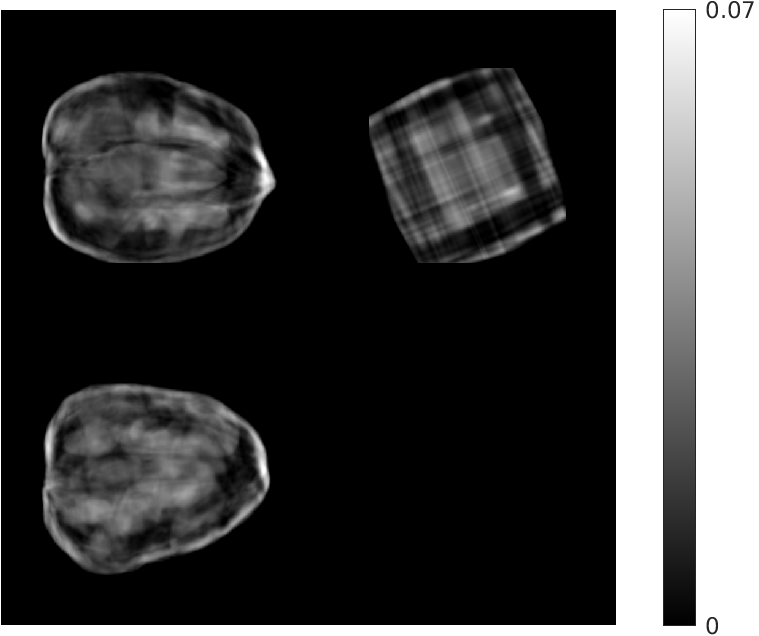
(b) (1.23)	(c) (0.65)
Destreaking CNN	Proposed
(d) (0.63)	(e) (0.45)

Figure 3: Comparison of the quality of reconstruction of our proposed algorithm (e) for walnut 2 (4 views) in Table I to various reference methods. Each subfigure depicts slices through the center of the walnut volume in the sagittal, coronal and transverse orientations. The normalized mean absolute errors have also been shown underneath each subfigure.

Fig. 4 shows the results of the intermediate steps of the first stage of our reconstruction for walnut 2 (8 views) in the test dataset. While the patch-based destreaking compensates for the blurring introduced by the EP-regularized reconstruction and ‘fills-in’ details in the reconstructed volume, the data-consistency plays a key role in mitigating hallucinations introduced by the CNN, and reinforces image features that are consistent with the acquired measurements.

Input EP Recon.	Post CNN-based Destreaking	Post Data-consistency
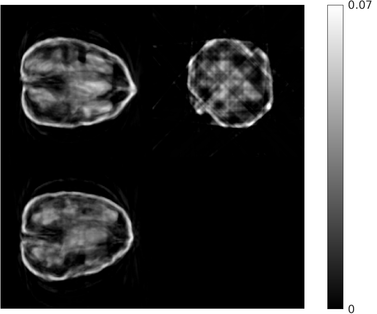
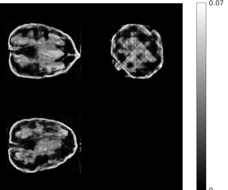
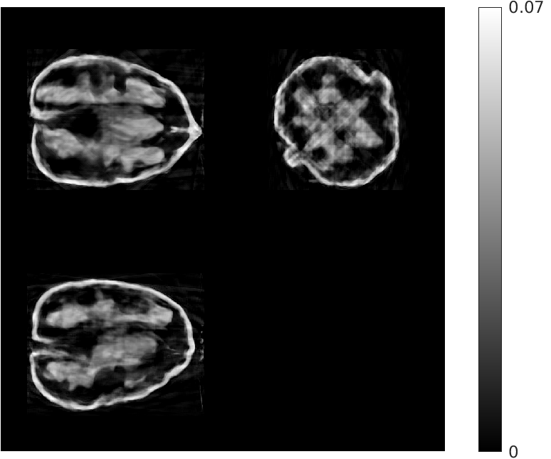
(NMAE:0.45)	(NMAE:0.38)	(NMAE:0.32)

Figure 4: Central slices corresponding to all three orientations of test walnut 2 (8 views) after various steps during a single stage (Stage 1) of our proposed algorithm.

Fig. 5 shows walnut 1 from our test dataset being progressively reconstructed from 8 projections across the stages of our algorithm; as the stages progress, more features are restored in the reconstructed walnut, until the improvements become incremental. The residual streaking artifacts outside the walnut are mitigated in the reconstructions from the third and fourth stages.

Stage 1	Stage 2
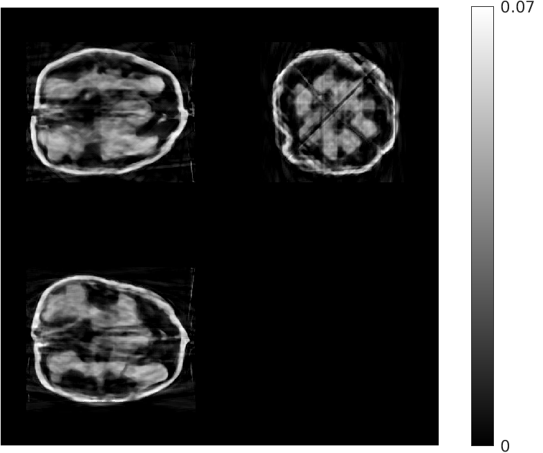
(a) (MAE: 0.32)	(b) (MAE: 0.29)
Stage 3	Stage 4
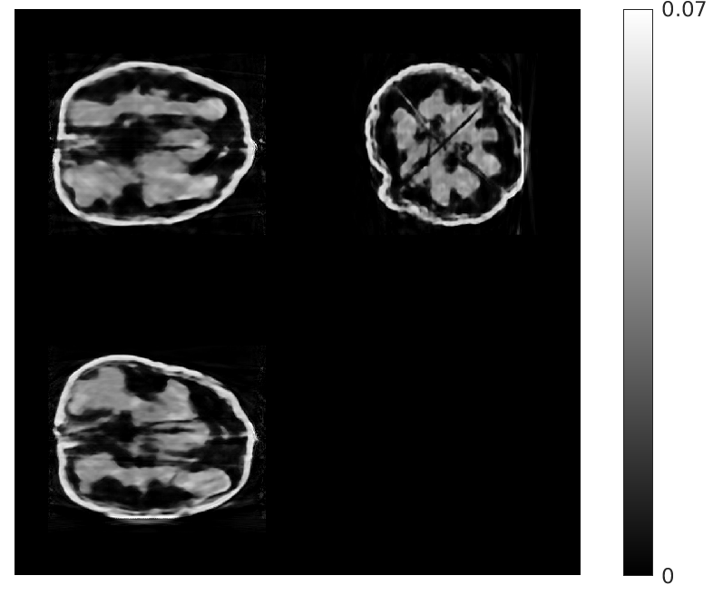
(c) (MAE: 0.27)	(d) (MAE: 0.26)

Figure 5: Central slices through the reconstructions of walnut 1 (8 views) in all three orientations at the end of each of the 4 stages of our algorithm (post data-consistency). It is evident that the quality of the reconstruction progressively improves across the stages. The normalized mean absolute error (NMAE) for each figure is also provided underneath

Fig. 6 (a) and (b) show how the quality of the reconstructions from 8 acquired views using our method varies when the orientation of the test walnuts is changed, in comparison to training-time. This is achieved by changing the position of the acquired (equidistant) projections, as this is akin to rotating the test walnut. For this purpose, essentially the position of the first acquired projection is shifted by a specified angle. For the three test walnuts shown in the figure, the angle of rotation was changed between +22.5°and -22.5°in intervals of 7.5°. Both the normalized mean absolute error (NMAE) and the normalized high-frequency error norm (NHFEN) were used as quality metrics in this experiment. Our method seems to be fairly robust to rotated test-data.

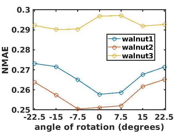
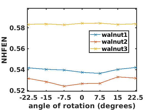
(a)	(b)
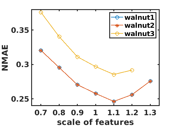
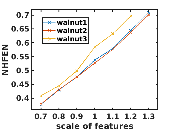
(c)	(d)

Figure 6: (a) and (b) show the effects of rotating the test walnuts (by changing the angle of acquired projections) on the quality of the reconstructions for 8 acquired views, while (c) and (d) capture the effect of varying the scale of features of the test walnut compared to the scale used in training. (a) and (c) depict the normalized MAE metric while (b) and (d) depict the normalized HFEN error metric for respective experiments.

We also studied the effect of varying the scale of the features of test walnuts on reconstructions from our method (from 8 projections), which was still trained on a single scale. For this purpose, we used the three walnuts which were used in the previous experiment. From Fig. 6 (c) and (d), it is evident that while there are differences in the NMAE and NHFEN across scales, our method holds up reasonably well across multi-scale test data. Particularly, we notice that while higher-frequency features are better reconstructed when the test walnuts are scaled down, the best NMAE is observed when the scale of the test walnut is 1.1 times its original scale. We surmise that this happens because at a scale of 1.1, the scale of features of the test walnuts matches that of the training walnut very well. (We excluded scale 1.3 for walnut 3 because at that scale, the walnut exceeded the $501\times 501\times 501$ voxel grid.)

V Discussion

Our observations in Section IV indicate that the proposed physics-aware learning-based approach for limited-view CBCT reconstruction is able to improve upon the quality of reconstructions yielded not only by the FDK algorithm, but also traditional prior-based iterative reconstruction, which serves a crucial role in initializing our algorithm, and ensures that the subsequent CNN-based destreaking is afforded a reasonable mapping to learn when trained with ground truth images as targets. Furthermore, in Fig. 4, we also demonstrated the importance of data-consistency when reconstructing from limited measurements. The data consistency update could easily be the most crucial step in our algorithm because it corrects for hallucinations introduced by the CNN-based destreaking step, which are very likely to occur given the limited availability of training data. This allows our algorithm to be repeated for several stages, which is key to the improvement provided by the proposed method over a simple image domain CNN-based denoiser. The generalizability of our approach is evident from the consistent improvements yielded by our approach in Table I, which is a consequence of using subvolumes or patches in training our method as well as the relative shallowness of the CNNs used therein. These measures effectively reduce the chances of overfitting when training on extremely limited full-view data. The chosen patch size effectively allowed the learned destreaking CNN to utilize three-dimensional context while also reducing: (1) the total number of overlapping subvolumes that are forward propagated through the destreaking CNN at test time and (2) the memory requirements for training the network. The hybrid 3D to 2D mapping also plays an important role by reducing the computational and time demands of our algorithm, and by removing any chances of artifacts that may be introduced during (conventional overlapping) patch aggregation.

We noted that the final reconstruction quality for some test walnuts was better than others, and also that the final reconstruction quality from our algorithm depended on the quality of the initial EP reconstruction. We think this may be because the acquired views (equidistant over $360^{\circ}$) may not be the best choice for higher fidelity reconstructions for some walnuts, and because these walnuts may be less similar to the training walnut.

Regarding the performance of our reconstructions in terms of the NHFEN metric, we observe a lack of sensitivity with respect to other compared techniques for both 8 and 4 views. We surmise that this is because neither of the networks was trained for improved NHFEN, i.e., a NHFEN term was not part of the training loss.

While the experiments with rotated projections and varying scale of features showcased some robustness of our proposed approach to both rotation and up/downscaling of features– it also brought to light the necessity for data augmentation for improved performance. The consistent degradation of the high frequency features (observed through the NHFEN metric) in reconstructions with increase in scale was interesting to note, and its contrast with the trends in NMAE points towards a sharpness/fidelity trade-off that may need more investigation.

However, it is key to realize that the improved performance in the NHFEN metric at smaller scales using our method is likely due to fewer edges that need to be reproduced in the image, and does not suggest that reconstructions of increasingly sharper quality may be obtained by continually shrinking the scale of walnuts.

VI Conclusions and Future Work

This paper developed a method to provide high quality reconstructions from extremely limited CBCT projections and scarce training data. The key features of our approach were the multi-stage approach of alternating between learning-based destreaking and data consistency and the use of subvolume-based learning and shallower (adversarially trained) CNNs to combat over-fitting. In the future, we will focus on extending our method to dynamic imaging applications in CT, as well as being able to jointly segment and reconstruct three-dimensional objects. Towards this end, we are also interested in finding a better metric than the mean absolute error to assess the fidelity and quality of our reconstructions for specific tasks.

The code for reproducing the results in this paper will be available on github after the paper is accepted.

References

- [1] L. A. Feldkamp, L. C. Davis, and J. W. Kress, “Practical cone beam algorithm,” J. Opt. Soc. Am. A, vol. 1, no. 6, pp. 612–9, Jun. 1984.
- [2] J.-B. Thibault, K. Sauer, C. Bouman, and J. Hsieh, “A three-dimensional statistical approach to improved image quality for multi-slice helical CT,” Med. Phys., vol. 34, no. 11, pp. 4526–44, Nov. 2007.
- [3] J. Xu and B. M. W. Tsui, “Interior and sparse-view image reconstruction using a mixed region and voxel-based ML-EM algorithm,” IEEE Trans. Nuc. Sci., vol. 59, no. 5, pp. 1997–2007, Oct. 2012.
- [4] J. H. Cho and J. A. Fessler, “Regularization designs for uniform spatial resolution and noise properties in statistical image reconstruction for 3D X-ray CT,” IEEE Trans. Med. Imag., vol. 34, no. 2, pp. 678–89, Feb. 2015.
- [5] G. Wang, “A perspective on deep imaging,” IEEE Access, vol. 4, pp. 8914–24, Nov. 2016.
- [6] I. Y. Chun, X. Zheng, Y. Long, and J. A. Fessler, “Sparse-view X-ray CT reconstruction using regularization with learned sparsifying transform,” in Proc. Intl. Mtg. on Fully 3D Image Recon. in Rad. and Nuc. Med, 2017, pp. 115–9.
- [7] I. A. Elbakri and J. A. Fessler, “Statistical image reconstruction for polyenergetic X-ray computed tomography,” IEEE Trans. Med. Imag., vol. 21, no. 2, pp. 89–99, Feb. 2002.
- [8] K. Sauer and C. Bouman, “A local update strategy for iterative reconstruction from projections,” IEEE Trans. Sig. Proc., vol. 41, no. 2, pp. 534–48, Feb. 1993.
- [9] J. A. Fessler, “Statistical image reconstruction methods for transmission tomography,” in Handbook of Medical Imaging, Volume 2. Medical Image Processing and Analysis, M. Sonka and J. M. Fitzpatrick, Eds. Bellingham: SPIE, 2000, pp. 1–70.
- [10] J.-B. Thibault, C. A. Bouman, K. D. Sauer, and J. Hsieh, “A recursive filter for noise reduction in statistical iterative tomographic imaging,” in Proc. SPIE 6065 Computational Imaging IV, 2006, p. 60650X.
- [11] A. R. De Pierro, “On the relation between the ISRA and the EM algorithm for positron emission tomography,” IEEE Trans. Med. Imag., vol. 12, no. 2, pp. 328–33, Jun. 1993.
- [12] S. Ravishankar, J. C. Ye, and J. A. Fessler, “Image reconstruction: from sparsity to data-adaptive methods and machine learning,” Proc. IEEE, vol. 108, no. 1, pp. 86–109, Jan. 2020.
- [13] S. Ahn, S. G. Ross, E. Asma, J. Miao, X. Jin, L. Cheng, S. D. Wollenweber, and R. M. Manjeshwar, “Quantitative comparison of OSEM and penalized likelihood image reconstruction using relative difference penalties for clinical PET,” Phys. Med. Biol., vol. 60, no. 15, pp. 5733–52, Aug. 2015.
- [14] W. Yu, C. Wang, X. Nie, M. Huang, and L. Wu, “Image reconstruction for few-view computed tomography based on sparse regularization,” Procedia Computer Science, vol. 107, pp. 808–813, 2017, advances in Information and Communication Technology: Proceedings of 7th International Congress of Information and Communication Technology (ICICT2017).
- [15] C. Xu, B. Yang, F. Guo, W. Zheng, and P. Poignet, “Sparse-view CBCT reconstruction via weighted Schatten p-norm minimization,” Opt. Express, vol. 28, no. 24, pp. 35 469–35 482, Nov 2020.
- [16] X. Zhang, Y. Zhou, W. Zhang, J. Sun, and J. Zhao, “Adaptive Prior Patch Size Based Sparse-View CT Reconstruction Algorithm,” in 2020 IEEE 17th International Symposium on Biomedical Imaging (ISBI), 2020, pp. 1–4.
- [17] Y. Kim, H. Kudo, K. Chigita, and S. Lian, “Image reconstruction in sparse-view CT using improved nonlocal total variation regularization,” in Developments in X-Ray Tomography XII, vol. 11113, International Society for Optics and Photonics. SPIE, 2019, pp. 329–337.
- [18] R. Anirudh, H. Kim, J. J. Thiagarajan, K. A. Mohan, K. Champley, and T. Bremer, “Lose the views: limited angle CT reconstruction via implicit sinogram completion,” in Proc. IEEE Conf. on Comp. Vision and Pattern Recognition, 2017, pp. 6343–52.
- [19] Y. Han, J. Kang, and J. C. Ye, “Deep learning reconstruction for 9-view dual energy CT baggage scanner,” in Proc. 5th Intl. Mtg. on Image Formation in X-ray CT, 2018, pp. 407–10.
- [20] H. Kim, R. Anirudh, K. A. Mohan, and K. Champley, “Extreme few-view ct reconstruction using deep inference,” arXiv preprint arXiv:1910.05375, 2019.
- [21] E. Y. Sidky, K.-M. Kao, and X. Pan, “Accurate image reconstruction from few-views and limited-angle data in divergent-beam CT,” J. X-Ray Sci. and Technol., vol. 14, no. 2, pp. 119–39, 2006. [Online]. Available: http://iospress.metapress.com/content/1jduv1cll3f9e2br/(notfree)
- [22] H. Yu and G. Wang, “Compressed sensing based interior tomography,” Phys. Med. Biol., vol. 54, no. 9, pp. 2791–806, May 2009.
- [23] J. Bian, J. H. Siewerdsen, X. Han, E. Y. Sidky, J. L. Prince, C. A. Pelizzari, and X. Pan, “Evaluation of sparse-view reconstruction from flat-panel-detector cone-beam CT,” Phys. Med. Biol., vol. 55, no. 22, p. 6575, Nov. 2010.
- [24] S. Ramani and J. A. Fessler, “A splitting-based iterative algorithm for accelerated statistical X-ray CT reconstruction,” IEEE Trans. Med. Imag., vol. 31, no. 3, pp. 677–88, Mar. 2012.
- [25] G. T. Herman and R. Davidi, “Image reconstruction from a small number of projections,” Inverse Prob., vol. 24, no. 4, p. 045011, Aug. 2008.
- [26] G.-H. Chen, J. Tang, and S. Leng, “Prior image constrained compressed sensing (PICCS): A method to accurately reconstruct dynamic CT images from highly undersampled projection data sets,” Med. Phys., vol. 35, no. 2, pp. 660–3, Feb. 2008.
- [27] L. Pfister and Y. Bresler, “Model-based iterative tomographic reconstruction with adaptive sparsifying transforms,” in Proc. SPIE 9020 Computational Imaging XII, 2014, p. 90200H.
- [28] C. Zhang, T. Zhang, M. Li, C. Peng, Z. Liu, and J. Zheng, “Low-dose CT reconstruction via L1 dictionary learning regularization using iteratively reweighted least-squares,” BioMedical Engineering OnLine, vol. 15, no. 66, 2016.
- [29] X. Zheng, S. Ravishankar, Y. Long, and J. A. Fessler, “PWLS-ULTRA: An efficient clustering and learning-based approach for low-dose 3D CT image reconstruction,” IEEE Trans. Med. Imag., vol. 37, no. 6, pp. 1498–510, Jun. 2018.
- [30] H. Chen, Y. Zhang, Y. Chen, J. Zhang, W. Zhang, H. Sun, Y. Lv, P. Liao, J. Zhou, and G. Wang, “LEARN: Learned experts: assessment-based reconstruction network for sparse-data CT,” IEEE Trans. Med. Imag., vol. 37, no. 6, pp. 1333–47, Jun. 2018.
- [31] D. Wu, K. Kim, G. E. Fakhri, and Q. Li, “Iterative low-dose CT reconstruction with priors trained by artificial neural network,” IEEE Trans. Med. Imag., vol. 36, no. 12, pp. 2479–86, Dec. 2017.
- [32] I. Y. Chun, H. Lim, Z. Huang, and J. A. Fessler, “Fast and convergent iterative image recovery using trained convolutional neural networks,” in Allerton Conf. on Comm., Control, and Computing, 2018, pp. 155–9, invited.
- [33] I. Y. Chun, Z. Huang, H. Lim, and J. A. Fessler, “Momentum-Net: Fast and convergent iterative neural network for inverse problems,” 2019. [Online]. Available: http://arxiv.org/abs/1907.11818
- [34] S. Ye, Z. Li, M. T. McCann, Y. Long, and S. Ravishankar, “Unified Supervised-Unsupervised (SUPER) Learning for X-Ray CT Image Reconstruction,” IEEE Transactions on Medical Imaging, vol. 40, no. 11, pp. 2986–3001, 2021.
- [35] A. Lahiri, G. Wang, S. Ravishankar, and J. A. Fessler, “Blind primed supervised (BLIPS) learning for MR image reconstruction,” IEEE Trans. Med. Imag., vol. 40, no. 11, pp. 3113–24, Nov. 2021.
- [36] G. Ongie, A. Jalal, C. A. Metzler, R. G. Baraniuk, A. G. Dimakis, and R. Willett, “Deep learning techniques for inverse problems in imaging,” IEEE Journal on Selected Areas in Information Theory, vol. 1, no. 1, pp. 39–56, may 2020.
- [37] M. Hossain, B. T. Nadiga, O. Korobkin, M. L. Klasky, J. L. Schei, J. W. Burby, M. T. McCann, T. Wilcox, S. De, and C. A. Bouman, “High-precision inversion of dynamic radiography using hydrodynamic features,” 2021. [Online]. Available: http://arxiv.org/abs/2112.01627
- [38] E. T. Quinto, “Exterior and limited-angle tomography in non-destructive evaluation,” Inverse Problems, vol. 14, no. 2, p. 339, 1998.
- [39] S. Guan, A. A. Khan, S. Sikdar, and P. V. Chitnis, “Limited-view and sparse photoacoustic tomography for neuroimaging with deep learning,” Scientific reports, vol. 10, no. 1, pp. 1–12, 2020.
- [40] M. Xiang, “Deep learning-based reconstruction of volumetric CT images of vertebrae from a single view X-ray image,” 2020, theses and Dissertations. 2629. University of Wisconsin Milwaukee. [Online]. Available: https://dc.uwm.edu/etd/2629
- [41] A. Ziabari, D. H. Ye, S. Srivastava, K. D. Sauer, J. Thibault, and C. A. Bouman, “2.5D deep learning for CT image reconstruction using A multi-GPU implementation,” in asccs, 2018, pp. 2044–9.
- [42] H. Lim, I. Y. Chun, Y. K. Dewaraja, and J. A. Fessler, “Improved low-count quantitative PET reconstruction with a variational neural network,” IEEE Trans. Med. Imag., vol. 39, no. 11, pp. 3512–22, Nov. 2020.
- [43] G. Corda-D’Incan, J. A. Schnabel, and A. J. Reader, “Memory-efficient training for fully unrolled deep learned PET image reconstruction with iteration-dependent targets,” IEEE Trans. Radiation and Plasma Med. Sci., 2021.
- [44] M. Magnusson, P.-E. Danielsson, and J. Sunnegardh, “Handling of long objects in iterative improvement of nonexact reconstruction in helical cone-beam CT,” IEEE Trans. Med. Imag., vol. 25, no. 7, pp. 935–40, Jul. 2006.
- [45] V. Monga, Y. Li, and Y. C. Eldar, “Algorithm unrolling: interpretable, efficient deep learning for signal and image processing,” IEEE Sig. Proc. Mag., vol. 38, no. 2, pp. 18–44, Mar. 2021.
- [46] H. Nien and J. A. Fessler, “Relaxed linearized algorithm for faster X-ray CT image reconstruction,” in Proc. Intl. Mtg. on Fully 3D Image Recon. in Rad. and Nuc. Med, 2015, pp. 260–3. [Online]. Available: http://web.eecs.umich.edu/~fessler/papers/files/proc/15/web/nien-15-rla.pdf
- [47] I. J. Goodfellow, J. Pouget-Abadie, M. Mirza, B. Xu, D. Warde-Farley, S. Ozair, A. Courville, and Y. Bengio, “Generative adversarial networks,” 2014. [Online]. Available: http://arxiv.org/abs/1406.2661
- [48] Y. Long, J. A. Fessler, and J. M. Balter, “3D forward and back-projection for X-ray CT using separable footprints,” IEEE Trans. Med. Imag., vol. 29, no. 11, pp. 1839–50, Nov. 2010.
- [49] H. D. Sarkissian, F. Lucka, M. . Eijnatten, G. Colacicco, S. B. Coban, and K. J. Batenburg, “A cone-beam X-ray computed tomography data collection designed for machine learning,” Sci. Data, vol. 6, p. 215, 2019.
- [50] J. A. Fessler, “Michigan image reconstruction toolbox (MIRT) for Matlab,” 2016, available from http://web.eecs.umich.edu/ fessler/irt/irt.
- [51] S. Ravishankar and Y. Bresler, “MR image reconstruction from highly undersampled k-space data by dictionary learning,” IEEE Trans. Med. Imag., vol. 30, no. 5, pp. 1028–41, May 2011.