Improving Time and Position Resolutions of RPC detectors using Time Over Threshold Information

Abstract

INO-ICAL is a proposed underground experiment to study the oscillation parameters of neutrinos by detecting those produced in the atmospheric air showers. The Iron CALorimeter (ICAL) is to have 151 layers of iron plates stacked vertically corresponding to a height of $\sim$14.5 m, with active detector elements inserted between the iron layers. The iron layers will be magnetized with a maximum magnetic field of 1.5 T to enable the measurement of the charge and momentum of the $\mu^{-}$ (or $\mu^{+}$) produced by $\nu_{\mu}$ (or $\bar{\nu}_{\mu}$) interactions inside the detector throughout the operation. Resistive Plate Chambers (RPCs) have been chosen as the active detector elements as they are amenable to large area coverage, as well as due to their high particle detection efficiency, long-term performance and low cost of production. The major factors that weigh in on the physics potential of the ICAL detector are the efficiency, position resolution and time resolution of the large area RPCs. A prototype detector called mini-ICAL (with 11 iron layers) was commissioned in order to understand the engineering challenges in building the large-scale electromagnet and its ancillary systems, and also to study the performance of the RPC detectors and readout electronics developed by the INO collaboration. As part of the performance study of the RPC detectors, an attempt is made to improve their position and time resolutions. The designed position resolution for the ICAL detector is of the order of 1 cm and the required time resolution is $\sim$1 ns. Even a small improvement in the position and time resolution will help to improve the measurements of momentum and directionality of the neutrinos in the ICAL detector. In ICAL detector simulation, where muons traverse in all directions with on average 20 RPC layers, a 30 $\%$ improvement in position resolution results in $\sim$10 $\%$ improvement in the momentum resolution at 3 GeV. Due to large iron materials in between two RPCs, the resolution is dominated by the effect of multiple scattering at this momentum. Also for a muon with 10 layer hit, the charge ambiguity reduces from 0.04 $\%$ to 0.001 $\%$ when the time resolution improves from 1 ns to 0.7 ns. The Time-over-Threshold (ToT) of the RPC pulses is recorded by the readout electronics. ToT is a measure of the pulse width and consequently the pulse amplitude. This information is used to improve the time and position resolution of RPCs and consequently INO’s physics potential.

1 Introduction

The proposed 50 k-ton magnetized Iron CALorimeter (ICAL) at the India-based Neutrino Observatory (INO) is planned to house underground at Bodi West Hill (South India) with a minimum of 1 km rock cover in all directions [1]. The ICAL detector can improve the measurements of the neutrino oscillation parameters such as $sin^{2}\theta_{23}$, and also the sign and value of |$\Delta m^{2}_{32}$|. Determining the sign of $\Delta m^{2}_{32}$ is one of the main goals of the ICAL experiment. The ICAL detector will be of 48 m $\times$ 16 m $\times$ 14.5 m in size and will be built as three independent modules of size 16 m $\times$ 16 m $\times$ 14.5 m, each module with 151 layers of 5.6 cm thick iron plates, which are vertically stacked and leaving 4 cm gaps between them. The Iron plates act as target mass for neutrino interactions as well as core material for the magnetic field. About 30000 Resistive Plate Chambers (RPCs) of $\sim$1.75 m$\times$1.85 m each will be housed in the gaps, for the tracking of charged particles through the detector and thus for momentum and direction measurement. As such ICAL is the only proposed neutrino detector, which can differentiate between $\nu_{\mu}$ and $\bar{\nu}_{\mu}$ simultaneously through the observation of $\mu^{-}$ and $\mu^{+}$ respectively. The neutrino mass hierarchy will indicate whether it is neutrinos or antineutrinos oscillation probabilities that will show MSW resonance [2] due to coherent forward elastic scattering in the matter on the earth. At this resonance condition, either $\nu_{\mu}$ or $\bar{\nu}_{\mu}$ oscillation to other flavours would be maximum.

It is also very important to resolve the "up-down ambiguity", i.e. whether the neutrino came from the top of the atmosphere or was travelling through the earth [1]. The timing information is important to resolve the up-down ambiguity of muons produced in the neutrino interactions. The RPC is chosen as the active layer due to its good timing resolution and low cost of manufacturing. The fraction of events reconstructed in the wrong direction drastically increases at lower energies, as the produced muon will cross only a few layers of ICAL [3]. Therefore an improvement in time resolution will further reduce the up-down ambiguity. Since the neutrinos arriving from different directions will encounter different path lengths in the earth, it is very important to also determine the direction (angular resolution) of the muon with very high precision. Position resolution plays a significant role in momentum resolution as well as angular resolution, both are required for the determination of the mass hierarchy.

Improving the position and time accuracy of the particle detectors is a never ending attempt - every generation of particle detectors improves upon the previous generation. The time resolution of Trigger RPCs is of the order of 1 ns. Compared to the older wire-based gaseous detectors, the uniform electric field in the RPC helps to eliminate the time jitter introduced by the non-uniform electric field in the latter. The avalanche in the RPC starts instantly, whereas this is not the case for wire-based detectors [4]. The Multi-Gap RPC [5], which has a time resolution of the order of 100 ps or less, is not a practical choice for ICAL considering the cost to make $\sim$30000 RPCs of size $\sim$1.75 m $\times$ 1.85 m. Therefore efforts are made to improve the time resolution of RPCs with the help of other information like the efficiency, signal multiplicity, etc.

In the current prototyping stage of ICAL, a stack named mini-ICAL with 11 layers of Iron plates and RPCs in between them is built at the transit campus of the Inter-Institutional Centre for High Energy Physics (IICHEP) at Madurai [6]. The mini-ICAL was commissioned in 2018 and started taking cosmics data by the middle of 2018. In comparison with the previous prototyping stage where a stack is built without the iron plates, the electronics are modified to store the Time-over-Threshold (ToT) information also. The use of ToT is more or less similar to the pulse height/integrated charge for the correction of timing, which is commonly used in the Multigap Resistive Plate Chamber (MRPC) [7]. All RPCs have an efficiency of $\sim$85$\%$ on average [6]. Section 2 describes the prototype setup used for this study. The event selection and data analysis are explained in Section 3. Section 4 briefly discusses the sources of the time resolution in RPCs. The discussion on the reflection of the signal, ToT, and using ToT for the correction of timing are given in Section 5. Along with the improvement of time measurement, the technique is also explored to improve the position resolution which is explained in Section 7. The ultimate goal of the reduction of the up/down ambiguity is discussed in Section 8. The effect of the terminator resistance on ToT performance is discussed in Section 9 and finally, the conclusions are drawn in Section 10.

2 Experimental Setup

The experimental setup as shown in Fig 1 (a) is a miniaturized version of ICAL, called mini-ICAL, with just 11 layers of iron plates with 10 RPCs between them. The mini-ICAL setup consists of 2 such stacks. The size of iron layers in mini-ICAL is 4 m $\times$ 4 m $\times$ 0.056 m. The total mass of mini-ICAL is 85 ton. The industrial production of the iron plates did not assure the required flatness. Hence the iron plates are stacked one above another with a gap of 4.5 cm in contrast to the original design of a 4 cm gap, which in turn ensured the easy installation of RPCs. Large area (175 cm $\times$ 185 cm) RPCs are placed in gaps. RPCs with the same dimensions are planned for the main INO-ICAL detector. There are two stacks of RPCs in the centre of the magnet system, each stack contains 10 RPCs, which are aligned vertically and this work is based only on the front stack. The placement of RPCs along with the layer numbering scheme is shown in Fig 1 (b).

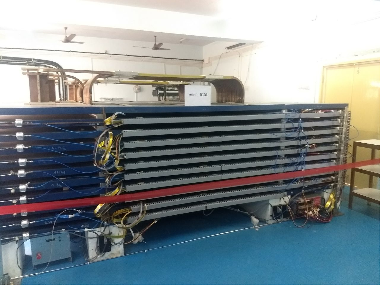
Figure 1: Fully Assembled mini-ICAL: (a) The front view of mini-ICAL (b) Schematic showing the location of RPCs inside mini-ICAL.

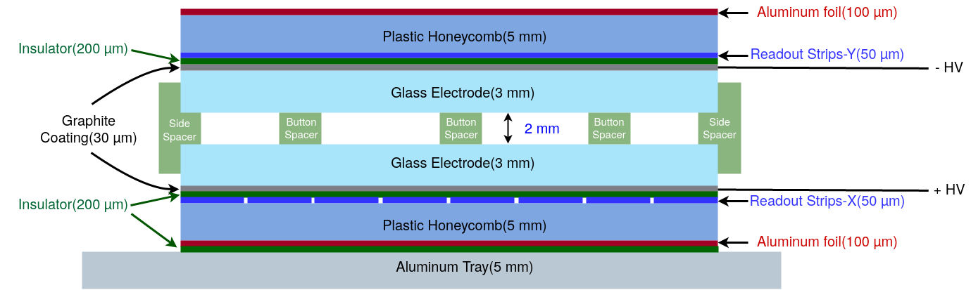
Figure 2: The schematic view of the RPC detector. The thickness of various components are shown.

The schematic view of the RPC in mini-ICAL is shown in Fig. 2. RPCs are made by placing two thin glass plates of size 175 cm$\times$185 cm and 3 mm thickness, placed 2 mm apart from each other. The bulk resistivity of glass used is 3-4$\times$10${}^{12}\Omega$cm [8]. The gap between the two glass plates is maintained to be 2 mm using circular poly-carbonate "button" spacers of diameter 11 mm. RPCs in layers 5, 7, 9 have 81 spacers, and all the remaining layers have 64 spacers placed as shown in Fig. 3. The sides are sealed with side spacers, forming a chamber. The fully assembled RPC is shown in Fig. 4. There are two sets of inlet and outlet nozzles through which the gas mixture is flown. The outer surfaces of the glass chamber are coated with a thin film of graphite paint. The graphite paint is applied by the screen printing technique. The surface resistivity of the graphite coat is in the range of 0.6-1.5 M$\Omega/\square$. This graphite coating permits the application of high voltage across the chamber as well as allows induced electrical signals to pass through it. The RPCs are operated at different high voltages based on the efficiency plateau using the muon data [9].

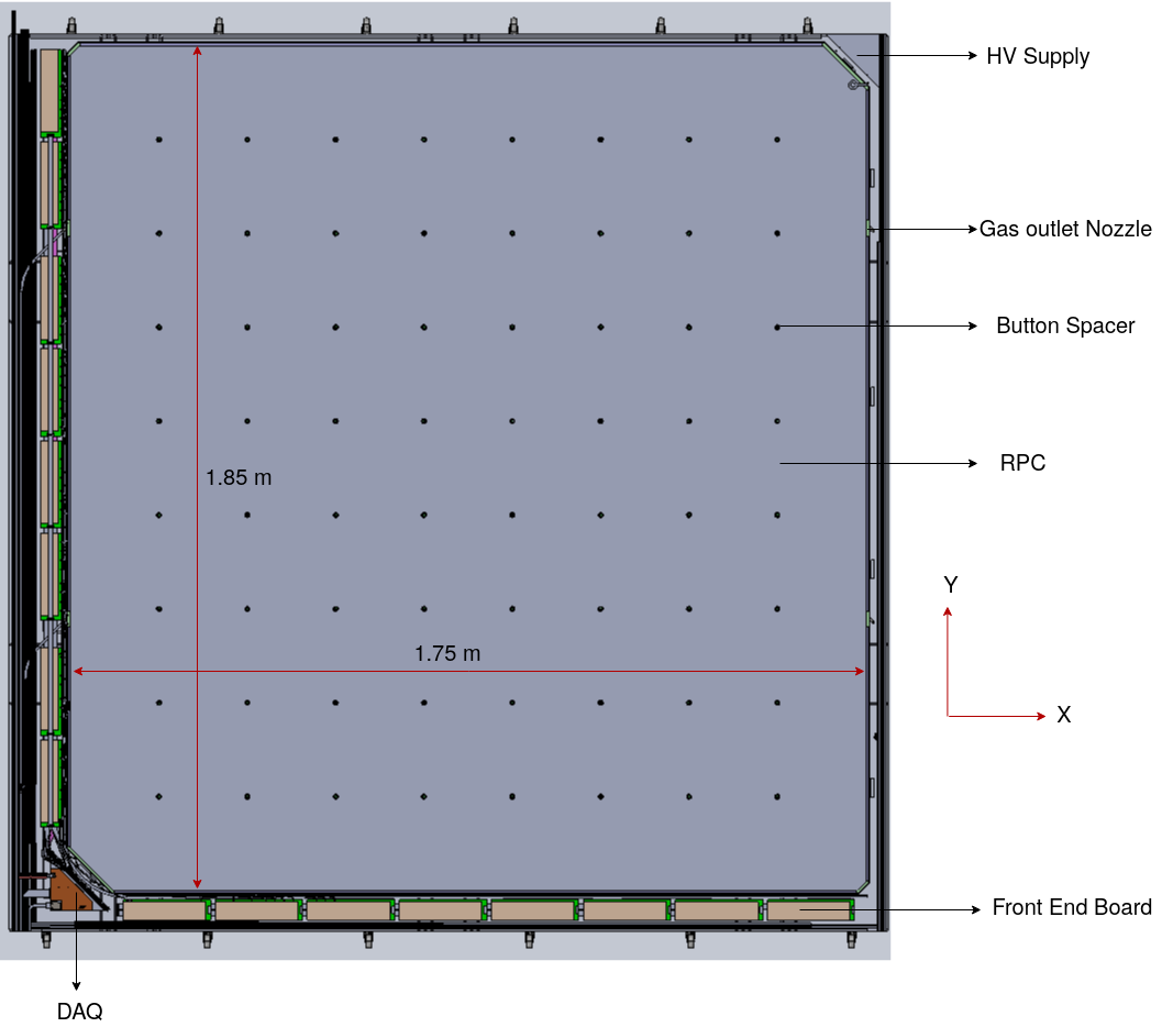
Figure 3: The top view of the RPC detector placed in a tray with the Front-End Board, Data Acquisition System and High Voltage Supply mounted.

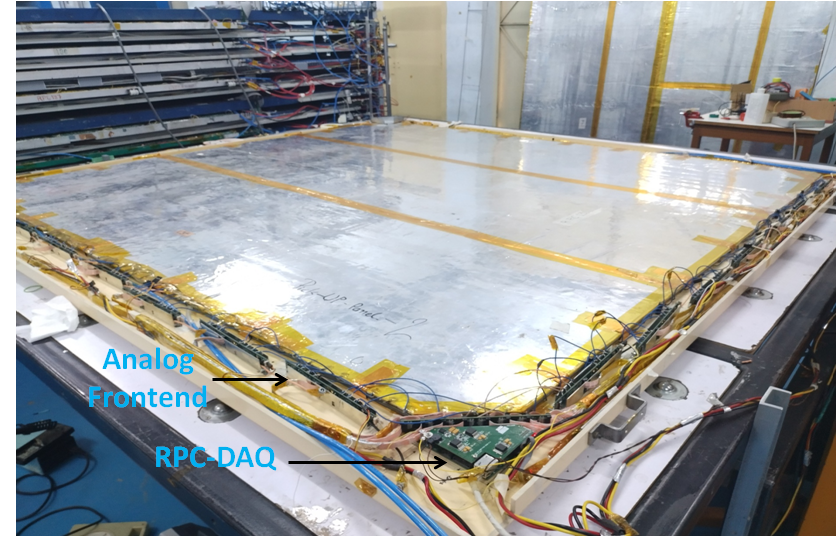
Figure 4: Fully Assembled RPC along with the tray.

The applied high voltage for optimum performance varies from 9.8 kV to 10.2 kV for different RPCs. A thin layer (100 $\mu$m) of two Mylar sheets (insulator) is kept in between the chamber and pick-up panels on both sides. The pick-up panel is made of copper (readout) strips with a width of 2.8 cm and an inter-strip gap of 0.2 cm pasted on a plastic honeycomb structure. The other side of the pick-up panel is pasted with thin aluminum foil and is connected to the ground. This will act as a Faraday cage for the strips. The readout strips are placed orthogonally on either side of the RPC to locate the position of the traversed particle. There are a total of 58 strips on the X-Side (bottom pickup panel) and 61 strips on the Y-Side (top pickup panel). The RPCs are operated in avalanche mode with a gas mixture of C₂H₂F₄ (95.2 $\%$), iso-C₄H₁₀ (4.5 $\%$), SF₆(0.3 $\%$). The gas mixture is continuously flowing through the chamber in an open loop with a flow rate of 6 standard cubic cm (sccm) per chamber.

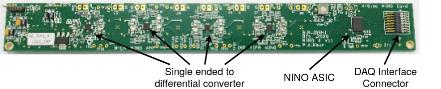
Figure 5: The Analog Front End Board.

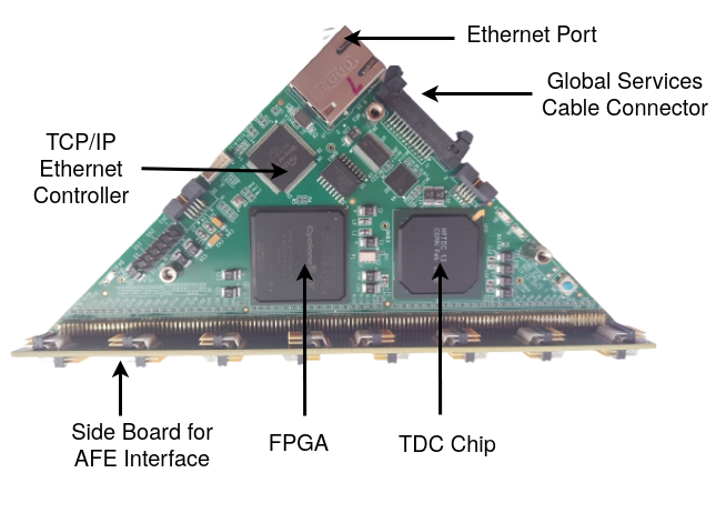
Figure 6: The Digital Front End Board.

The induced signals are amplified and discriminated by an 8-channel NINO ASIC chip [10]. The discriminator in the NINO is kept at a threshold of 100 fC. To identify as signals of traversing charged particles over background noise, the signal in a strip over this threshold is defined as “hit”. The hit localization is done using the information from the strips in both planes. Each chamber has 119 electronic channels (58 X-strips and 61 Y-strips) requires 16 NINO chips, so a total of 160 NINO chips are used. Since the NINO is designed to accept differential signals, the single-ended signals from the RPC strips were converted into differential signals and fed to the NINO chip. The Analog Frontend Board with this single-ended to differential converters and the NINO ASIC is shown in Fig. 5. The LVDS output of NINO is fed to the FPGA-based RPC data acquisition system, which is located at one corner of the RPC tray as shown in Fig. 3 via 100 $\Omega$ twisted-pair cable. The Digital Front End module consists of several functional blocks such as Time-to-Digital Converter(TDC), Strip-hit latch, Pre-trigger generator, Rate Monitor, Front End control and ambient parameter monitor as shown in Fig.6. The time resolution of TDC is 100 ps. A pre-trigger signal was generated by the OR of all strips on either the X-side or Y-side. The pre-trigger signals from the FPGA-based DAQ boards are fed to Signal Router Boards (SRBs), which bunch signals and redistribute them to Trigger Logic Boards (TLBs) as shown in Fig. 7. In Fig. 7 only one of the RPC is shown for simplicity, but there are 10 RPCs with the corresponding Front End Boards and RPC-DAQ boards. A second-level trigger for cosmic muons was created by requiring the coincidence of pre-trigger signals in layers 6, 7, 8 and 9 within the time window of 100 ns. Events with either an X-side or a Y-side trigger are stored. Once the trigger is formed the digitized data is transmitted to the back-end using the DAQ boards network interface [11]. The efficiency measurements performed on this setup are described in [6].

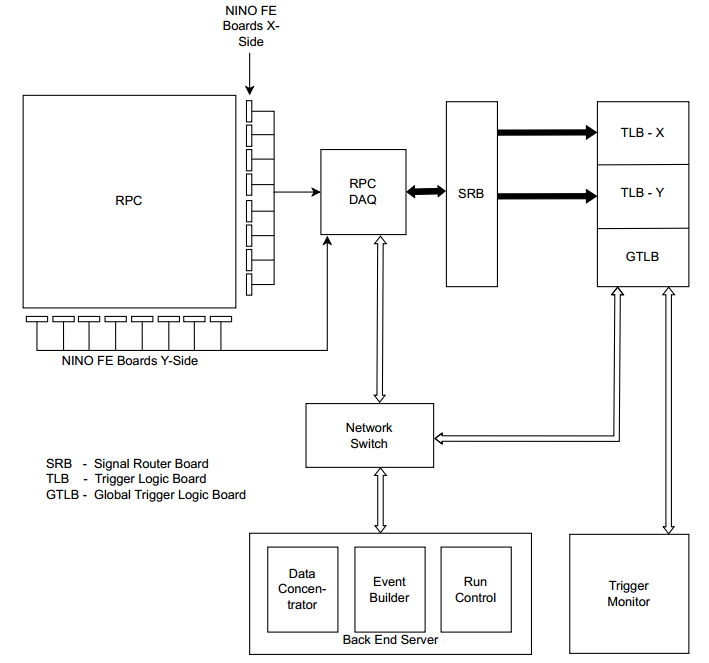
Figure 7: The Data Acquisition System.

The detector is magnetized using two copper coils as shown in Fig 1 (b), by passing $\sim$900 A through each coil generating a uniform field of 1.5 T in the negative Y direction where RPCs are situated. The temperature in the coil is maintained with the help of a closed-loop low conductivity water cooling system. For the current study, the magnet was switched OFF.

3 Event Selection and Data Analysis

The data used for this analysis is taken during December 2018, contains $\sim$9.2 million events and corresponds to 14 hours 20 minutes of run time with a trigger rate of $\sim$180 Hz. The hardware trigger records events with hits in four fixed trigger layers within a coincidence time window. This recorded data contains the single muon events, as well as events with multiple trajectories due to hadronic showers and electronic noise. Sample events of these two types are shown in Fig. 8. The hadrons can give a shower of hits, which may create multiple trajectories and create separate clusters in many layers. On the other hand in general the tracks created by single muons won’t create many clusters in a layer, even though the hits would be in consecutive strips due to sharing of induced charge and other correlated electronic noise. With these considerations, a layer that has only one cluster and with cluster-size$\leq$3 is selected explicitly for a good position resolution [12]. The above criterion also eliminates the shower events and the layers with outliers mainly due to electronic noise. The study in this paper is performed using only the single muon events. The induced signal due to the single muon gives clear trajectories and the strip multiplicity is less than four for the avalanche signal. The cluster-size for selected muon events where at least 6 layers are used to find the muon trajectory and considering the hits within only $\pm$20 ns of the muon time is shown in Fig. 9. For these distributions, first a hit is linked with the muon trajectory and then the consecutive hits are clustered together after removing dead strips in the strip list.

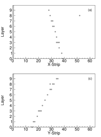
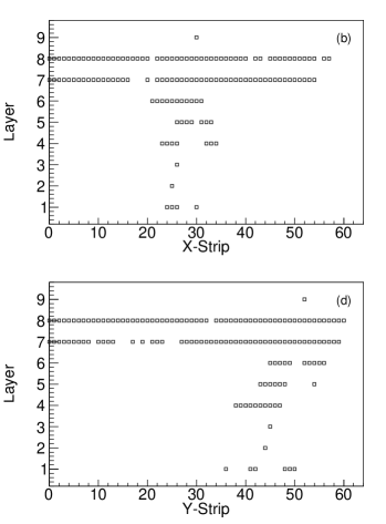
Figure 8: Example of a single muon event: (a) X-plane (c) Y-plane. Example of hadron tracks: (b) X-plane (d) Y-plane.

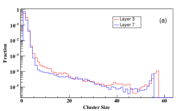
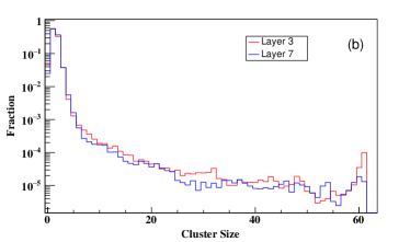
Figure 9: Clustersize of muon events for layer 3 and layer 7: (a) X-Side (b) Y-Side.

3.1 Position Analysis

The selected hits from different layers are fitted using the equation of straight line  3.1 in XZ- and YZ-views independently.

$$x\,(\,\mathrm{or}\>y)=\alpha\times z+\beta~{}$$ (3.1)

where the x/y and z are X/Y-position and the layer height from the bottom layer. The parameters, $\alpha$ and $\beta$ are the slope and intercept. Information about the trajectory is calculated by combining the fit parameters from the XZ- and YZ-view separately. Before proceeding to the detailed analysis, the time offset corrections were done using the recorded muon data. The residual distance is defined as the distance between the hit and the extrapolated hit position. The residual distribution is expected to be Gaussian with a mean at zero. The deviation of the mean from zero denotes there is an offset of the position of this RPC relative to other layers. To calculate the unbiased position correction for each layer, an iterative procedure is followed. In the iterative procedure, a layer is not included in the fit, the trajectory position is estimated using the fit parameters using other layers. After 4-5 iterations, the position accuracy of less than 100 $\mu m$ is achieved [13].

3.2 Time Analysis and Existing Time Corrections

After fitting the position information, the valid strip hits (within 6 cm of the fit position) are selected for the time correction.

Using the information from position fit, the timing information of muons is extracted from the reading in the corresponding TDC channel. For hits with cluster-size greater than 1, the strip with the earliest time is considered for the time information of that layer. The selected time information is fitted using again the straight line Eqn. 3.2,

$$t_{x/y}=\frac{1}{v}l_{i}+\delta~{}$$ (3.2)

where the $t_{x/y}$ is the time information from the X- or Y-plane, $v$ is the velocity, $l_{i}$ is the track length in the $i^{th}$ layer and the $\delta$ is the constant time offset due to trigger timing. Similar to the estimation of the offsets for the position, the time corrections are also essential to obtain a more precise measurement of time resolution. There are already a set of corrections that are calculated offline and the details of these corrections are discussed in Ref. [13]. For the completeness of this paper, in brief, the existing corrections are:

• Correction for the signal propagation delay from the position where muon crossed the RPC to the front-end board.

• The strip-wise time offset corrections for all the strips in the X- and Y-plane, due to different cable lengths for the readout of the various strips.

• The time correction as a function of the position within the strip for strip multiplicity of more than one.

4 Various contributions to the time resolution

Times are recorded independently on the top (Y-side) and bottom (X-side) pick-up panels of all RPCs. The uncertainties of the measurement in X- and Y-side are mainly categorized into two parts, $(i)$ uncorrelated and $(ii)$ correlated sources.

4.1 Uncorrelated sources

The uncorrelated sources are (i) the individual electronic components, e.g., gain in pre-amplifiers, jitter in discriminator, (ii) the signal pick-up on X-and Y-plane may differ due to the air gap between the gas gap and pick-up panel, which can cause the walk in the timing, (iii) the non-uniformity of the surface resistivity of the coating may cause different spread in the induced signal and (iv) position of the induced signal with respect to the centre of the X- and Y-strip. The offline corrections will take care of the mean time shift in each strip and as well as pixel (3 cm$\times$3 cm area, matching the pitch of the strip). Correcting the jitter due to the electronics in the X- and Y-plane on an event-by-event basis is not possible. Also due to the uncertainty on the extrapolated trajectory in a layer, the uncertainty due to the (iv)-th source can not be eliminated completely.

4.2 Correlated sources

The correlated sources of time spread are mainly contributed from two major sources, $(i)$ the fluctuation in the starting of an avalanche causes variation in the gain, which will create the spread in the observed time and $(ii)$ the walk in the discriminated signal due to different pulse height also creates the spread in the timing. Case (i) cannot be corrected because this is intrinsic. But the case (ii) can be corrected in a few ways, for example, the Constant Fraction Discriminator (CFD) can solve the walk in the discriminated signal. To reduce the complexity of the electronics the existing setup does not have CFD. But, the electronics is equipped to store the time difference between the leading and the trailing edge of the signal above the threshold as the width of LVDS output, which can be used for correcting the time walk.

5 Timing Correction with Time Over Threshold Information

The output of the front-end chip NINO will give a pseudo-LVDS signal (discriminated pulse), the width of this pulse is proportional to the time over threshold (ToT) of the RPC pulse. ToT is also correlated with the charge from the pick-up strips. The variation of pulse width with respect to the input charge is non-linear. The variation in pulse width is larger for lower pulses and is smaller for higher pulses. The pulse width variation versus input charge is shown in Ref. [14]. This pulse width for different pulse heights can be used to correct the time walk.

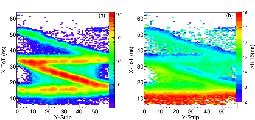
Figure 10: (a) The distribution of X-ToT vs Y-strip. (b) The time shift calculated in each bin of (a).

Figure 11: The observed pulse reflection from the RPC strips and schematic of the reflection between front-end and termination resistor.

To check the dependency of the pulse width on the position along the pick-up strip, the distribution of pulse width from the X-plane versus muon position in the Y-plane is shown in Fig. 10(a). The distribution shows four distinct bands. The same is observed in the Y-plane also as a function of the muon position in the X-plane. The first (bottom) band is the expected band corresponding to the signal at the pre-amplifier, provided no reflection from the termination resistance opposite side of the signal pick-up. The other bands are coming from the reflection of the signal due to the impedance mismatch with the termination at both ends of the strip. The RPC signals are readout only on one side of the strip, the other side of the strip is terminated using a 47 $\Omega$ resistor. The specific value of the termination resistors was chosen based on the preliminary measurements performed using sample pick-up panels during the pre-production. But the observation using the muon data tells that the characteristic impedance of the pick-up panels used in the prototype stack has to be less than 47 $\Omega$. The input impedance of the front-end is around 56 $\Omega$, which is also more than the pick-up panel, so this also will cause reflection in the front-end. Fig. 10(a) shows that there are a large fraction of events whose ToT is modified due to multiple reflections. The correlation of ToT and threshold crossing time is obliterated due to the reflections from improper termination. The reflections due to the termination resistor and the front-end leading to the distinct bands are explained in Fig. 11. If one part of the signal travel towards the front-end amplifier and the other part travel towards the termination resistor, the pulse width will depend inversely on the distance from the front end (second band). If the induced signal is large enough the reflected pulse crosses the threshold of the discriminator. And if the induced signal is even larger, the signal traveling toward the front end amplifier is reflected twice and will be able to cross the discriminator threshold. In this case, the pulse width will increase by a constant value, which is twice the time taken for the signal to propagate from one end of the strip to the other end. That is the reason why the slope of the third band is zero. The fourth band is due to a signal with three reflections for a much larger signal and that band has the same slope as the second band.

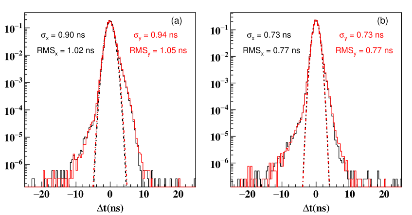
Figure 12: Time residual distributions for Layer-3 before the removal of positions where spacers are there from the analysis (a) before ToT corrections, (b) after correction with ToT.

The observed reflections in data can not be removed unless the terminator resistances change. The average time shift for each bin in figure 10(a) is calculated from the observed data, which is the mean of the distribution obtained by taking the difference between the observed time and the expected time from equation 3.2. Depending on the ToT and the position in a strip, this shift is applied to correct for the time-walk. The calculated average values are shown in figure 10(b) as a 2D histogram where the bin content shows the time shift to be applied as the correction. In the plot, an addition of 15 ns is done to have all average points on the positive side for the visualization. The mean shifts from each bin can be used for correction in further analysis.

The time residual distribution for a layer is obtained by taking the time difference between the measured time hit and the expected time hit after fitting the measured times of layers other than that under study using equation 3.2. The time residual plot obtained without and with the above mentioned correction shows a large deviation from a gaussian distribution at a leading time as shown in figure 12 . This is predominantly attributed to the spacer positions[13]. For all the subsequent analysis, a $6\,cm\times 6\,cm$ area is removed in the vicinity of the spacers to avoid the bias due to those hits. This corresponds to a $\sim$10$\%$ decrease in the statistics for 81 spacer RPCs and a $\sim$7$\%$ decrease in the statistics for 64 spacer RPCs.

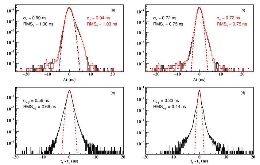
Figure 13: Time residual distributions for Layer-3 after removing the positions where spacers are there from the analysis (a) before ToT corrections, (b) after correction with ToT. (c) and (d) are the observed time difference between the X- and Y-plane before and after ToT corrections.

The time residual distributions for layer-3 before and after correcting the ToT with pixel-wise time shift correction and also removing the spacer positions is shown in figure 13(a) and 13(b) respectively. There is a clear reduction of tails on the negative side of the distributions.

The fit was done using the time and position information of the layers other than the layer under study. The events selected for the analysis have to have at least 6 layer hits where the layer under study is omitted. The implementation of the pulse width correction improved the measurement of the time resolution of the RPC detectors. This is seen in the shape of the distribution on the right side even after ToT corrections. In 13(a) the right side shoulder is due to signals, which are small and cross the discriminator threshold at a later time. This shoulder is substantially reduced in 13(b) after incorporating the ToT corrections. Similarly, the difference between the time measurement in the X- and Y-plane ($t_{x}-t_{y}$) is shown in 13(c) and 13(d) without and with the ToT correction respectively. It is assumed that the uncorrelated errors in the X- and Y-side are the same and for further studies, the uncorrected error on either side are taken as $(1/\sqrt{2})\,\sigma$, where $\sigma$ is the width of the Gaussian fit parameter.

The time resolution for different RPC layers before and after ToT correction for X-and Y-plane are given in table 1 and table 2 respectively, where "ExtErr" is the average extrapolated error due to the error in the fit parameters, "$\sigma$" is the observed Gaussian fitted width of the $\Delta t$ distribution, "Corr $\sigma$" is the time resolution of the RPC chamber after subtracting the extrapolation error for each layer, "Uncorr Err" is the uncorrelated error in time measurement for individual side obtained from the Gaussian fit of the $t_{x}-t_{y}$ distributions and "Correlated $\sigma$" is the estimated error on corrected time resolution after subtracting the extrapolation and uncorrelated error.

Table 1: The time resolution (ns) for X-plane in different RPC layers before and after ToT corrections.

Layer		Before ToT correction				After ToT correction
	Ext Err	$\sigma$	Corr. $\sigma$	Uncorr Err	Correlated $\sigma$	$\sigma$	Corr. $\sigma$	Uncorr Err	Correlated $\sigma$
0	0.612	1.221	1.057	0.546	0.905	0.949	0.725	0.339	0.641
1	0.511	1.179	1.062	0.534	0.918	0.868	0.702	0.322	0.623
2	0.401	1.174	1.103	0.648	0.893	0.836	0.733	0.363	0.637
3	0.355	0.897	0.824	0.403	0.719	0.719	0.625	0.238	0.578
4	0.284	0.878	0.831	0.442	0.703	0.697	0.636	0.286	0.568
5	0.262	0.969	0.933	0.437	0.824	0.687	0.635	0.256	0.581
6	0.285	0.958	0.915	0.472	0.784	0.706	0.646	0.294	0.576
7	0.343	1.002	0.941	0.473	0.813	0.753	0.671	0.288	0.605
8	0.438	1.047	0.951	0.449	0.838	0.794	0.662	0.275	0.603
9	0.570	1.125	0.970	0.562	0.790	0.866	0.652	0.288	0.585

Table 2: The time resolution (ns) for Y-plane in different RPC layers before and after ToT corrections.

Layer		Before ToT correction				After ToT correction
	Ext Err	$\sigma$	Corr. $\sigma$	Uncorr Err	Correlated $\sigma$	$\sigma$	Corr. $\sigma$	Uncorr Err	Correlated $\sigma$
0	0.617	1.264	1.103	0.546	0.959	0.944	0.714	0.339	0.628
1	0.507	1.224	1.114	0.534	0.977	0.886	0.726	0.322	0.651
2	0.405	1.158	1.085	0.648	0.870	0.795	0.684	0.363	0.580
3	0.357	0.935	0.864	0.403	0.765	0.716	0.621	0.238	0.574
4	0.286	0.938	0.894	0.442	0.777	0.708	0.648	0.286	0.582
5	0.267	0.997	0.961	0.437	0.855	0.709	0.657	0.256	0.605
6	0.294	1.002	0.958	0.472	0.834	0.724	0.661	0.294	0.593
7	0.355	1.064	1.003	0.473	0.884	0.784	0.699	0.288	0.636
8	0.454	1.075	0.974	0.449	0.864	0.818	0.680	0.275	0.622
9	0.585	1.209	1.057	0.562	0.896	0.897	0.680	0.288	0.617

For all the time residual distributions, improvement in the tail part is more after correcting for ToT. That is due to the effect of the position of muon trajectory in the strip coordinate. The muon might pass through the centre of X-strip, but at the edge of Y-strip and vice-versa. One expects a larger signal, consequently faster time while muon trajectory is at the center of the strip [13]. It is always the case that the layer under study is excluded from the fit. So while studying a layer before the ToT corrections are applied, the other layers in the fit are applied with ToT correction to improve the extrapolation error. Since the extrapolation error due to the fit is lower in the middle layers, the observed $\sigma$ are also lower for the middle layers. Even after the corrections, it looks like the errors in the middle layers are less than that in the uppermost and lowermost RPC layers. This could be due to the intrinsic properties of RPCs in different positions or due to any inherent bias in the fitting procedure. The last doubt is removed using MC simulated events, which will be described in the next section. The quoted uncorrelated errors also show a similar trend, which is taken from the difference in timing on the X- and Y-side of the strip and independent of any bias due to the fitting algorithm. The explanation of this trend could be due to better electromagnetic shielding of inner layers from external noises. But, overall the correlated error, which is dominated by the development of avalanche, is reduced from 0.70 - 0.98 ns to $\sim$ 0.57 - 0.64 ns, which is a big improvement in the time resolution measurement.

6 Systematic Uncertainties

For the baseline analysis, the minimum number of layers in the fit has to be greater than or equal to 6. There was no criterion placed to select the events based on $\chi^{2}/ndf$ criteria, either during time offset correction or for finding the resolution for individual layers, where $ndf$ is the number of degrees of freedom. The criteria on minimum number of layers for fitting, selecting good events for the correction of timing, etc., might bias the obtained results. Thus, after applying all the corrections on time, the hits with more than 5 ns from the muon time are removed for the next iteration of fitting to remove the effect of outliers. All these criteria reduce the statistics of timing distribution to $\sim$3 million entries in each layer. Fig. 14 shows the $\chi^{2}/ndf$ plot for X-Side and Y-Side fitting using 3.2 after corrections with ToT. A comparison of time resolutions obtained from data and from Monte Carlo simulations is explained in 6.1. The effect of $\chi^{2}/ndf$, number of layers in the fit and different offset corrections using selected events on the corrected $\sigma$ is studied in 6.2, 6.3 and 6.4 respectively. In order to verify the fitting procedure, the difference between the corrected time in different layers is studied in 6.5.

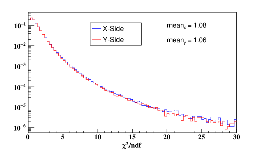
Figure 14: $\chi^{2}/ndf$ distribution of fit 3.2 in X-side and Y-side after ToT correction.

6.1 Monte Carlo simulation

The results of section 5 are verified with help of events simulated using GEANT4 toolkits and reconstructed using the same algorithm which was used to find the time resolution in data. The simulated hit time is smeared with a Gaussian in both X-Side and Y-Side, containing both correlated and uncorrelated parts. The correlated parts are matched exactly with the input value within the statistical uncertainties. The reconstructed results of uncorrelated error are also estimated with the same procedure in data and are compared with the input values, which are given in Tab. 3. There is a bias of about 10 ps in the measured time resolutions, which is much smaller than the variation of resolutions between different layers.

Table 3: Comparison of input and reconstructed timing resolution (ns) in simulation.

	Layer	0	1	2	3	4	5	6	7	8	9
Total	Input $\sigma$	0.725	0.702	0.733	0.625	0.636	0.635	0.646	0.671	0.662	0.652
	Fitted $\sigma_{x}$	0.718	0.698	0.738	0.620	0.635	0.627	0.649	0.663	0.653	0.647
	Fitted $\sigma_{y}$	0.713	0.704	0.736	0.617	0.628	0.626	0.642	0.658	0.639	0.638
Corre-lated	Input $\sigma$	0.641	0.623	0.637	0.578	0.568	0.581	0.576	0.605	0.603	0.585
	Fitted $\sigma_{x}$	0.635	0.615	0.642	0.571	0.563	0.570	0.576	0.597	0.589	0.577
	Fitted $\sigma_{y}$	0.629	0.622	0.639	0.568	0.555	0.570	0.569	0.590	0.574	0.567

6.2 Effect of $\chi^{2}/ndf$ on the corrected $\sigma$

In the baseline analysis, there was no criterion on $\chi^{2}/ndf$ of the fit to select the muon trajectories. The fit quality of the timing measurements might improve with the criterion on $\chi^{2}/ndf$ of the fit. The corrected $\sigma$ for different criteria on $\chi^{2}/ndf$ are shown in figure 15. This shows a shift in the correct $\sigma$ with the stronger criterion on $\chi^{2}/ndf$. This apparent bias is due to the inherent method of measurement. With the tighter criterion, a subset of events is selected which has less error on extrapolation, but the estimation of extrapolation error is based on $\chi^{2}/ndf<\infty$. Thus the over-estimation of extrapolation error in the selected events reduces the corrected $\sigma$. The is a systematic reduction of $\sigma$ with a tighter and tighter criterion of $\chi^{2}/ndf$ confirms the logic.

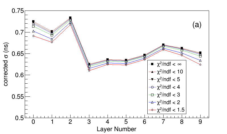
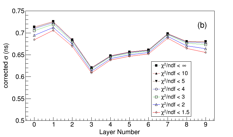
Figure 15: Corrected $\sigma$ calculated by putting various cuts on $\chi^{2}/ndf$ (a) for X-Side, (b) for Y-Side.

6.3 Effect of number of layers in the fit on the corrected $\sigma$

To have more statistics, the data were selected with the muon signal in at least six other layers excluding the test layer. The variation of the observed resolution with the variation of the minimum number of other layers in the fitting is shown in figure 16. Here also observed a systematic shift in the resolution for a few layers, while increasing the number of layers in the fit. By changing the number of layers in the fit from 6 to 8, the variation in corrected $\sigma$ is only 1.2 $\%$.

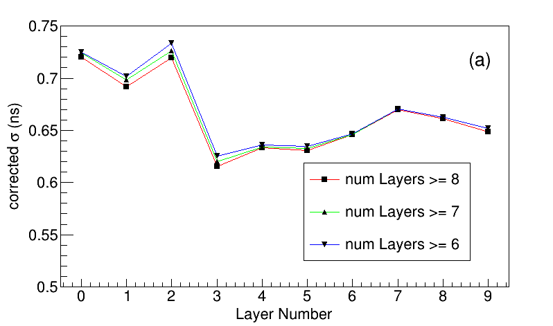
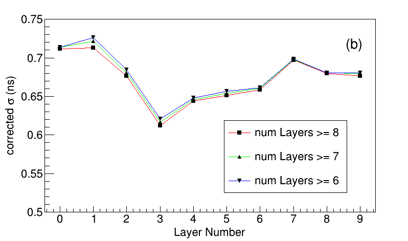
Figure 16: Corrected $\sigma$ calculated by putting various cuts on number of layers in the fit (a) for X-Side, (b) for Y-Side.

6.4 Effect of time offset with different ndf on the corrected $\sigma$

Initially, the time offset corrections were done using a minimum of 6 layers in the fit, where one expected larger uncertainties in the offset corrections. Another correction was done by using only longer tracks. Using a larger minimum number of layers in the fit reduces the statistics, which in turn deteriorates the measurement accuracy. As a trade-off, the offset corrections are done with events having at least 8 layers in fit along with criterion, $\chi^{2}/ndf<2$. The comparison of final results with these two sets of offset corrections is shown in figure 17, where the observed difference is much smaller in comparison with other effects.

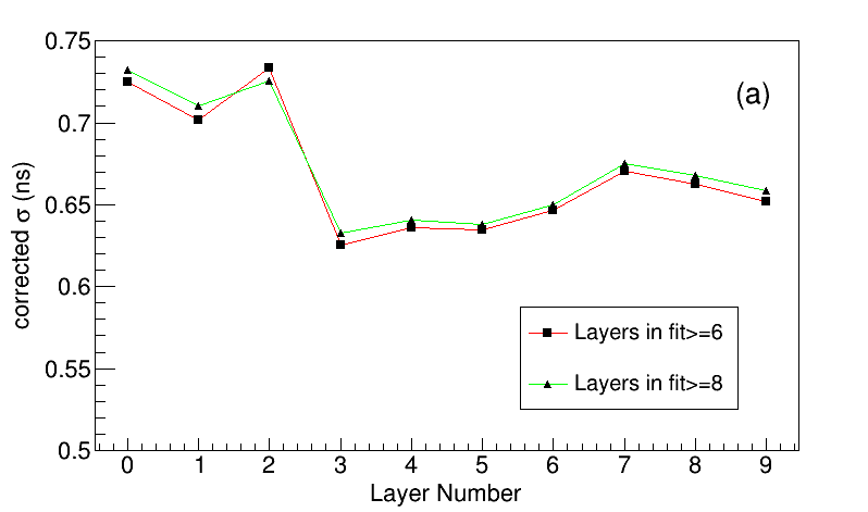
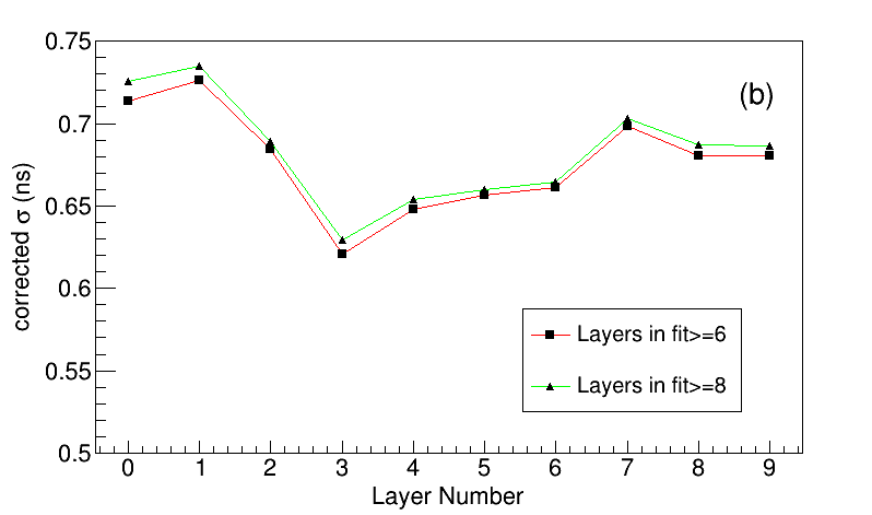
Figure 17: Corrected $\sigma$ calculated by putting various cuts on number of layers in the fit after time offset corrections with longer tracks (a) for X-Side, (b) for Y-Side.

6.5 Resolution using the muon time difference in different layers

In order to verify the corrected $\sigma$ obtained after subtracting the extrapolated error, the difference between muon time in different layers after the ToT corrections is used. After correcting the path length delay the width of difference between two layers should be equal to the quadratic sum of the corrected $\sigma$ in those layers. The time difference in Layer-3 & Layer-4 is shown in figure 18, where the observed sigma is exactly the quadratic sum of the resolution of those layers.

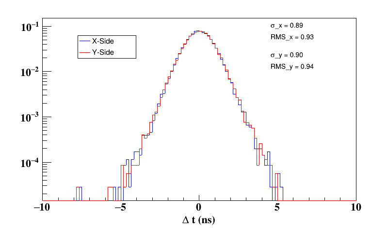
Figure 18: Time Difference between layer 3 and layer 4 after all the correction and also by taking care of the path length correction.

All possible combinations of time differences between layers are also used to find the time resolution of all individual layers. To obtain the individual resolution of the layers, we minimize the function S, where S is given by the expression,

$$S=\sum_{i=0}^{8}\sum_{j=i+1}^{9}\Big{(}\frac{\sigma_{i}^{2}+\sigma_{j}^{2}-\Delta_{ij}^{2}}{(\sigma_{{}_{\Delta_{ij}}})^{2}}\Big{)}^{2}$$ (6.1)

where $\Delta_{ij}$ is the width of the time difference distribution between layers i and j, $\sigma_{{}_{\Delta_{ij}}}$ is the error on the $\Delta_{ij}$ parameter. The errors on $\sigma_{i}$’s are avoided in the definition of S, because we are estimating the value of those $\sigma_{i}$’s. Any input to the error on $\sigma_{i}$’s might bias the minimization. Tab. 4 shows the obtained time resolution in different layers and in comparison with the values of the same quantities in Table 1 and 2 shows consistent results with a maximum deviation of 3%. But, there is no systematic bias in the estimated resolutions in these two procedures.

Table 4: The time resolutions (ns) for X-Plane and Y-Plane after the minimization of S.

Layer	0	1	2	3	4	5	6	7	8	9
Corrected $\sigma_{x}$	0.709	0.693	0.748	0.628	0.638	0.634	0.645	0.669	0.658	0.634
Corrected $\sigma_{y}$	0.695	0.717	0.685	0.628	0.650	0.656	0.658	0.689	0.673	0.664

6.6 Summary of the systematic studies

The variation of different systematic effects is summarized in table 5. The summary of the differences between the default results and the obtained results with the measurements described in the previous sections in 20 numbers (10 layers and both X- and Y-side) are given in the table. It is apparent there is no bias in the observed $\sigma$, except in the case of $\chi^{2}/ndf$ criteria, but the source of that bias is well understood. The systematic variations are smaller than the variation of the central values in different layers.

Table 5: Effect of different systematic error (ps) on the estimation of resolution.

	Mean	RMS of	Maximum +ve	Maximum $-$ve
	difference ($\mu$)	difference	shift from $\mu$	shift from $\mu$
Montecarlo	8.8	7.3	20.2	13.8
$\chi^{2}/ndf$	16.8	7.3	17.2	7.55
Number of layers	5.1	4.0	8.7	4.6
Offset correction	5.3	3.6	6.1	12.9
Time difference	4.3	8.5	14.7	19.3

7 Position Corrections using Time information

As the Time-over-Threshold information is used to improve the time resolution of RPCs, an attempt is also made to have an algorithm to improve the position resolution. The basic idea behind the technique is similar to the charge centroid method in wire chambers. The avalanche signal due to the passage of muon through the RPC can cause strip multiplicity up to three/four. The events with strip multiplicity between four to ten are primarily due to the streamer pulses and hadronic showers. The layers that have a strip multiplicity of more than ten are mainly due to correlated electronic noise. Thus, this study is restricted up to multiplicity three. When muon passes through the middle of two strips, the charge induced between the strips depends on the position where muon passes through. The charge shared between the strips can be extracted using the value of ToT. The improvement is possible only when the strip multiplicity is two or three. The new position correction in a layer is calculated with a trajectory position in that layer estimated by fitting the data from other layers. The corrections are calculated as a function of two parameters independently, ($i$) leading time and ($ii$) ToT corrected time. The lead time is the threshold crossing time of the leading part of the RPC pulses, which varies as the charge of the pulses varies. The smaller the charge, the threshold crossing time is delayed and vice versa.

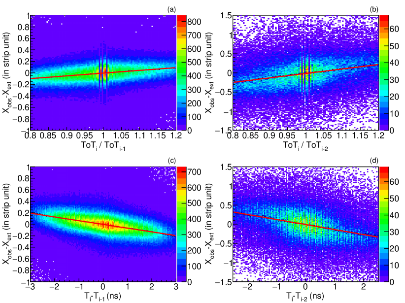
Figure 19: (a) and (b) are the distribution of the position corrections versus the ToT_i/ToT_i-j for strip multiplicity two and three respectively. (c) and (d) are the position corrections as a function of the T_i-T_i-j for strip multiplicity two and three respectively.

Figs. 19 (a) and (b) are the distribution of the position residuals versus the ToT_i/ToT_i-j for the strip multiplicity two and three respectively in layer-5. Figs. 19 (c) and (d) are the position residuals for the test RPC as a function of the $T_{i}-T_{i-j}$ (the difference between the lead time in $i^{th}$ strip and $j^{th}$ strip) for strip multiplicity two and three respectively again for the muons with minimum seven layers in the fit, where $i$ represents the rightmost (+ve side) strip among two/three strips $(i-1(2))$ is the leftmost ($-$ve side) strip with multiplicity two(three). The distribution shows that there is a clear correlation between the lead time of the signal and the position of the muon in the strip. The data points are fitted with a straight line and the fit parameters are later used in the event by event corrections. Similar to the lead time, the position corrections based on ToT are also done event by event during the analysis. The position residuals before any correction, the corrections using pulse width and lead time for events with strip multiplicity two are shown in Figs. 20 (a), (b) and (c) respectively. The position residuals before any correction and using the pulse width and lead time corrections for events with strip multiplicity three are shown in Figs. 21 (a), (b) and (c) respectively. The distribution is fitted with Gaussian and the $\sigma$ is considered to be a position resolution of the RPC.

There has been a reasonable improvement in the position resolution for strip multiplicity, two and three for the particular layer. In the figures $\sigma$ includes the extrapolation error also, hence it is larger than the intrinsic error. The corrections are not able to improve the tail part of the distribution, so there is relatively little change in RMS. We expect similar improvement in all other layers by these corrections. The strip multiplicity for muon trajectory is about 1.5, thus on average 33% of layers will have improved measurement of the position in the event since this correction is applied to multiplicity 2, and multiplicity 3 hits only.

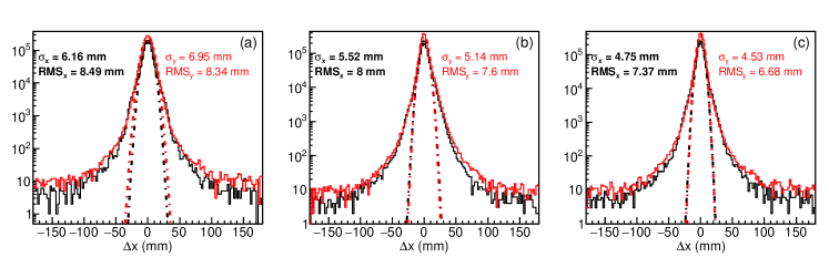
Figure 20: (a), (b) and (c) are the position residuals before any correction, pulse width corrections and lead time corrections respectively for events with hit multiplicity of two.

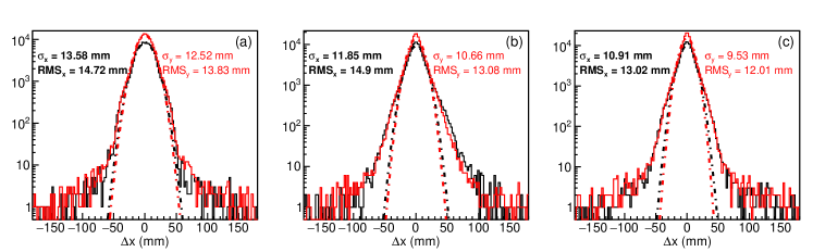
Figure 21: (a), (b) and (c) are the position residuals before any correction, pulse width corrections and lead time corrections respectively for events with hit multiplicity of three.

8 Identification of muon direction

The identification of muon direction is an important parameter in ICAL since this parameter is used to distinguish between up-going and down-going muons [1]. Fig 22, shows the time slope of the muon after fitting the time with distance. The Z-coordinate of the mini-ICAL is in the upward direction, but the cosmic muons are coming downward. The slope in the unit of ($-1/c$) reverses the direction of the muon and also normalizes the speed in the unit of $c$, the speed of light in vacuum. For an ideal case, this peak is at one and that is the observation. The slope with a negative value corresponds to muons misidentified to be going upward. The sample may contain some genuine up-going muons. But it’s assumed that the muons are only going downwards, neglecting the back-scattered muons and the muons produced by neutrinos coming from down. Fig 22 shows the fraction of maximum misidentified muon direction with numbers of layers in the fit shown in the figure, $\chi^{2}/ndf<2$ and also for various conditions as described below,

1. including the spacer positions and without ToT correction,

2. including the spacer positions and with ToT correction,

3. excluding the spacer positions and without ToT correction,

4. excluding the spacer positions and with ToT correction,

5. excluding the spacer positions and with ToT correction and also selecting vertical muons having zenith angle < 10^∘,

6. excluding the spacer positions and with ToT correction and $\chi^{2}/ndf<1.5$.

The effect of the spacer is prominent if the number of layers in the fit is less, and becomes insignificant as the number of layers in the fit increases. With the application of ToT corrections, the fraction of misidentified muons decreased. The misidentification ratio from this study cannot be compared with the previous studies [13, 3] because the maximum number of layers was 12 in those studies with more gap (16 cm) in between two layers. Those studies were done with a completely different prototype stack. Though the study of ToT correction was done by removing the spacer position, this result does not show any observed deterioration of fit/physics performance with the inclusion of that area. The muon trajectory near the spacer position has tails on the lower side of the $\Delta t$ distributions, but in the fit that is excluded if the observed point is more than 3 $\sigma$ away from the fitted value. Thus, the effect of the shift in timing near the spacer position does not affect much, though it is affected indirectly due to the reduction of an effective number of layers in the performance/physics study. Fig 22 (e) shows the effect of the path length on the maximum mis-identification fraction. Since the path length between layers is less for vertical muons, the mis-identification fraction is large. Fig 22 (f) shows the improvement in the maximum mis-identification fraction by selecting events with better fit quality.

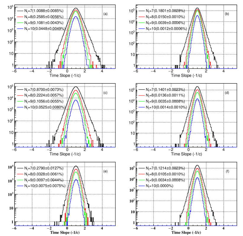
Figure 22: Slope of time fit is overlaid with different number of layers in the fit.(a),(c) without ToT corrections and (b),(d) with ToT Correction, (a),(b) with the spacer positions and (c),(d) removing the spacer positions. (e) is as the same condition as (d) but only events with zenith angle less than 10^∘ is considered and (f) is with a much tighter criteria of $\chi^{2}/ndf<1.5$ and the ToT corrections applied after removing spacer positions. The fraction of misidentified events are also given in percentage for different number of layers used in the fit.

9 Study of Reflections with Different Termination Resistors

To investigate the effect of impedance mismatch between the termination resistor and pick-up strips on pulse reflections, resistors with different values are connected in one of the RPC in standalone mode and all these tests were done just by inserting signals in different positions of the strip using a pulser. The result indicates the best matching with the termination resistance 18$\pm$3 $\Omega$ for different strips. Thus an RPC with different termination resistors is placed on top of the mini-ICAL (10th layer). The muon data were recorded based on the coincidence of the signals from the bottom four layers (6 to 9). For this study, the resistors with values of 15 $\Omega$ (0 to 19 strips in X- and Y-planes), 18 $\Omega$ (20 to 39 strips in X- and Y-planes) and 22 $\Omega$ (remaining strips in both X- and Y-plane) are used as the terminator of pick-up strips. The muon data recorded with this configuration is analyzed. The muon trajectories are selected with the criteria that at least seven RPC layers are used in the fit and $\chi^{2}/ndf$ of the fits are less than two individually both for X-Z and Y-Z planes. The distribution of the ToT vs positions along the strip for 15 $\Omega$, 18 $\Omega$ and 22 $\Omega$ are shown in Figs.23 (a), (b) and (c) respectively. It is observed that the contribution from the reflected pulses (in the same phase as the first pulse) is diminishing with the decrease in the termination resistor value. Also, it can be noted that there is a small fraction of the reflected component in the distribution even at 15 $\Omega$ termination resistor. Figs. 24 (a), (b) and (c) are the time offset calculated for using Bin-by-Bin of the ToT vs Position along the strip distribution for 15 $\Omega$, 18 $\Omega$ and 22 $\Omega$ respectively. There are almost linear correlations of ToT and the time shift for all three termination resistances.

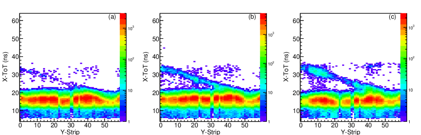
Figure 23: Correlation between the X-ToT and Y-strip position with termination resistance (a) 15 $\Omega$, (b) 18 $\Omega$ and (c) 22 $\Omega$ respectively.

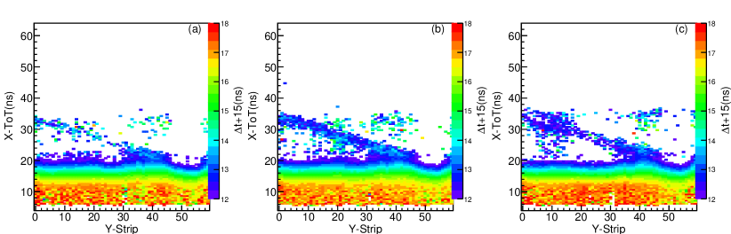
Figure 24: (a), (b) and (c) are the time offset distribution of X-ToT vs position along the Y-strip with termination resistance 15 $\Omega$, 18 $\Omega$ and 22 $\Omega$ respectively.

The time residual distribution after ToT correction for these three sets of termination resistors such as 15 $\Omega$, 18 $\Omega$ and 22 $\Omega$ are shown in Figs. 25 (a), (b) and (c) respectively. The 0 to 19th X-strips with termination resistance 15 $\Omega$ are overlapped for all strips on Y-side. Thus, $t_{x}-t_{y}$ is taken for only those events where both X- and Y- strips have the same termination resistor instead of mixing with all possible combinations of termination resistances.

All resolutions, with and without the ToT corrections are given in Table 6. There are small differences in the extrapolation errors in these three sets of data, which are mainly due to the non-uniformity of gain of RPCs in the mini-ICAL detector.

It is observed that the corrected time resolution after the Bin-by-Bin offsets does not differ much even if the termination resistors are changed. This result might be due to the fact that the values of three different resistances are nearest. To verify that this is not the case, one set of readings with the same conditions were taken by replacing all the three different resistors with 39 $\Omega$. The result is shown in Fig. 26. This corroborates that changing the termination resistor does not influence the ToT correction. This means that the walk in the larger pulses is not much, hence the saturation of pulse width at larger pulses does not contribute to time walk correction. The reason for the bumps seen on either side of the Gaussian part of $t_{x}-\textbf{ }t_{y}$ as seen in Fig. 25 is not clear and under further study.

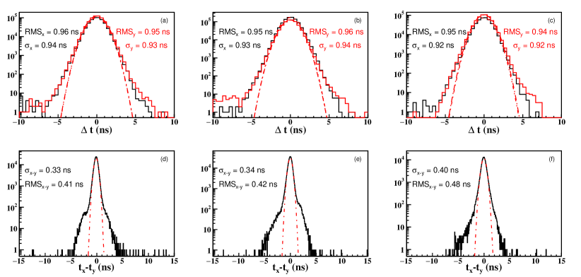
Figure 25: (a), (b) and (c) are the time residual distribution after ToT correction for strip with termination resistance 15 $\Omega$, 18 $\Omega$ and 22 $\Omega$ respectively. (d), (e) and (f) are the observed time difference between the X- and Y-plane after ToT corrections for both X $\&$ Y-strip with termination resistance 15 $\Omega$, 18 $\Omega$ and 22 $\Omega$ respectively.

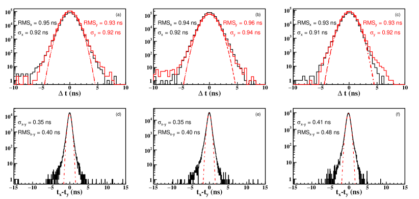
Figure 26: Time residual distributions with termination resistance 39 $\Omega$; (a), (b) and (c) are with ToT correction for both X,Y strips from 0-19, 20-39, 40-59 strip and (d), (e) and (f) are the observed time difference between the X- and Y-plane after ToT corrections for both X,Y strips from 0-19, 20-39, 40-59 respectively.

Table 6: Extrapolated error and the time resolution (in $ns$) before and after incorporating the ToT corrections for different termination resistances for the events with number of layers $\geq$ 6.

	X-Plane			Y-Plane			X-Plane			Y-Plane
Ter. Resistance	15 $\Omega$	18 $\Omega$	22 $\Omega$	15 $\Omega$	18 $\Omega$	22 $\Omega$	39 $\Omega$	39 $\Omega$	39 $\Omega$	39 $\Omega$	39 $\Omega$	39 $\Omega$
Ext Err	0.57	0.57	0.59	0.60	0.60	0.59	0.55	0.55	0.57	0.57	0.57	0.56
$\Delta t_{\mathrm{w.oToT}}$	1.36	1.30	1.38	1.38	1.39	1.42	1.39	1.30	1.38	1.39	1.39	1.43
$\Delta t_{\mathrm{withToT}}$	0.94	0.93	0.92	0.93	0.94	0.92	0.92	0.92	0.91	0.92	0.94	0.92
Corr $\Delta t_{\mathrm{w.oToT}}$	1.24	1.17	1.25	1.24	1.25	1.29	1.27	1.18	1.26	1.27	1.27	1.32
Corr $\Delta t_{\mathrm{withToT}}$	0.74	0.74	0.71	0.72	0.72	0.71	0.74	0.74	0.71	0.72	0.75	0.73

10 Conclusion

The 85-ton magnetized prototype of ICAL, called mini-ICAL is commissioned and operational. The muon data collected from the mini-ICAL is used to study the RPC performances like individual strip count rates, detector efficiency, position resolution, time resolution, etc. This work discussed the sources of the RPC time resolution and estimated the different sources. The time-walk in the discriminator due to the pulse height is corrected using the Time-Over-Threshold (ToT) information stored in the data and the time resolution is studied before and after ToT correction. The present technique of ToT correction is used to improve the time resolution of RPCs. The intrinsic resolution changed from $\sim$0.77 - 0.98 ns to $\sim$0.57 - 0.66 ns. Along with the improvement in the time resolution, the techniques are explored to improve the position accuracy of the RPC detector based on lead time and pulse width information. As a result of the corrections, there has been substantial improvement in the position resolution. Based on the knowledge gained from the mini-ICAL, the ToT information will be used in the ICAL experiment to correct the timing of signals. From the experience with this setup, the termination resistance will be chosen properly to avoid reflections of signal, though it does not show any visible effect in the physics performance.

References

- [1] S. Ahmed et. al., Physics Potential of the ICAL detector at the India-based Neutrino Observatory (INO), Pramana 88 (2017) 5, 79.
- [2] Mikheyev, S. P., Smirnov, A. Yuu, Resonance enhancement of oscillations in matter and solar neutrino spectroscopy, Sov.J.Nucl.Phys. 42 (1985) 913-917, Yad.Fiz. 42 (1985) 1441-1448, Wolfenstein, L., Neutrino oscillations in matter, Physical Review D17 (1978) 2369-2374.
- [3] G. Majumder, N.K. Mondal, S. Pal, D. Samuel, B. Satyanarayana, Study of the directionality of cosmic muons using the INO-ICAL prototype detector, Nucl. Instr. Meth. Phys. Res. A735 (2014) 88-93.
- [4] Christian Lippmann, Detector Physics of Resistive Plate Chambers, CERN-THESIS-2003-035.
- [5] E.C. Zeballos et. al., A new type of resistive plate chamber: The multigap RPC, Nucl. Instr. Meth. Phys. Res. A374 (1996) 132-135.
- [6] A.D. Bhatt Measuement of Atmospheric Muons at IICHEP in Madurai, for better estimation of Neutrino Fluxes at INO Site in Theni, PhD Thesis HBNI, Mumbai(2019).
- [7] A.V. Akindinov et. al., Results from a large sample of MRPC-strip prototypes for the ALICE TOF detector, Nucl. Instr. Meth. Phys. Res. A532 (2004) 611-621.
- [8] K. Raveendrababu et. al., Effect of electrical properties of glass electrodes on the performance of RPC detectors for the INO-ICAL experiment, Journal of Instrumentation11(2016) P08024
- [9] M. Abbrescia et. al., Beam test results on double-gap resistive plate chambers proposed for CMS experiment, Nucl. Instr. Meth. Phys. Res. A414 (1998) 135-148.
- [10] Achrekar S. et. al., Electronics, Trigger and Data Acquisition Systems for the INO ICAL Experiment. In: Liu ZA. (eds) Proceedings of International Conference on Technology and Instrumentation in Particle Physics 2017. TIPP 2017, Springer Proc.Phys. 212 (2018) 291-295.
- [11] M. N. Saraf et. al., Electronics and DAQ for the Magnetized mini-ICAL Detector at IICHEP, Springer Proc.Phys. 261 (2021) 779-786.
- [12] S. Pethuraj et. al., Measurement of azimuthal dependent muon flux by 2 m2 m RPC stack at IICHEP-Madurai, Experimental Astronomy 49 (2020) 141-147.
- [13] A.D. Bhatt et. al., Improvement of time resolution in large area single gap Resistive Plate Chambers, Nucl. Instr. Meth. Phys. Res. A844 (2017) 53-61.
- [14] F. Anghinolfi et. al., NINO: an ultra-fast and low-power front-end amplifier/discriminator ASIC designed for the multigap resistive plate chamber, Nucl. Instr. Meth. Phys. Res. A533 (2004) 183-187.