Revisiting Global Pooling through the Lens of Optimal Transport

Abstract

Global pooling is one of the most significant operations in many machine learning models and tasks, whose implementation, however, is often empirical in practice. In this study, we develop a novel and solid global pooling framework through the lens of optimal transport. We demonstrate that most existing global pooling methods are equivalent to solving some specializations of an unbalanced optimal transport (UOT) problem. Making the parameters of the UOT problem learnable, we unify various global pooling methods in the same framework, and accordingly, propose a generalized global pooling layer called UOT-Pooling (UOTP) for neural networks. Besides implementing the UOTP layer based on the classic Sinkhorn-scaling algorithm, we design a new model architecture based on the Bregman ADMM algorithm, which has better numerical stability and can reproduce existing pooling layers more effectively. We test our UOTP layers in several application scenarios, including multi-instance learning, graph classification, and image classification. Our UOTP layers can either imitate conventional global pooling layers or learn some new pooling mechanisms leading to better performance.

1 Introduction

As an essential operation of information fusion, global pooling aims to achieve a global representation for a set of inputs and make the representation invariant to the permutation of the inputs. This operation has been widely used in many machine learning models. For example, we often leverage a global pooling operation to aggregate multiple instances into a bag-level representation in multi-instance learning tasks (Ilse et al., 2018; Yan et al., 2018). Another example is graph embedding. Graph neural networks apply various pooling layers to merge node embeddings into a global graph embedding (Ying et al., 2018; Xu et al., 2018). Besides these two cases, global pooling is also necessary for convolutional neural networks (Krizhevsky et al., 2012; He et al., 2016). Therefore, the design of global pooling operation is a fundamental problem for many applications.

Nowadays, simple global pooling operations like mean-pooling (or called average-pooling) and max-pooling (Boureau et al., 2010) are commonly used because of their computational efficiency. The mixture and the concatenation of these simple operations are also considered to improve their performance (Lee et al., 2016). Recently, many pooling methods, $e.g.$, Network-in-Network (NIN) (Lin et al., 2013), Set2Set (Vinyals et al., 2015), DeepSet (Zaheer et al., 2017), attention-pooling (Ilse et al., 2018), and SetTransformer (Lee et al., 2019a), are developed with learnable parameters and more sophisticated mechanisms. Although the above pooling methods work well in many scenarios, their theoretical study is far lagged-behind — the principles of the methods are not well-interpreted, whose rationality and effectiveness are not supported in theory. Without insightful theoretical guidance, the design and the selection of global pooling are empirical and time-consuming, often leading to suboptimal performance in practice.

In this study, we propose a novel algorithmic global pooling framework to unify and generalize many existing global pooling operations through the lens of optimal transport. As illustrated in Figure 1(a), we revisit a pooling operation from the viewpoint of optimization, formulating it as optimizing the joint distribution of sample index and feature dimension for weighting and averaging representative “sample-feature” pairs. From the viewpoint of statistical signal processing, this framework achieves global pooling based on the expectation-maximization principle. We show that the proposed optimization problem corresponds to an unbalanced optimal transport (UOT) problem. Moreover, we demonstrate that most existing global pooling operations are specializations of the UOT problem under different parameter configurations.

By making the parameters of the UOT problem learnable, we design a new generalized global pooling layer for neural networks, called UOT-Pooling (or UOTP for short). Its forward computation corresponds to solving the UOT problem, while the backpropagation step updates the parameters of the problem. Besides implementing the UOTP layer based on the well-known Sinkhorn-scaling algorithm (Cuturi, 2013; Pham et al., 2020), we design a new model architecture based on the Bregman alternating direction method of multipliers (Bregman ADMM, or BADMM for short) (Wang & Banerjee, 2014; Xu, 2020), as shown in Figure 1(b). Each implementation unrolls the iterative optimization steps of the UOT problem, whose complexity and stability are analyzed quantitatively. In summary, the contributions of our work include three folds.

Modeling. To our knowledge, we make the first attempt to propose a unified global pooling framework from the viewpoint of computational optimal transport. The proposed UOTP layer owns the permutation-invariance property and can cover typical global pooing methods.

Algorithm. We propose a Bregman ADMM algorithm to solve the UOT problem and implement a UOTP layer based on it. Compared to the UOTP implemented based on the Sinkhorn-scaling algorithm, our BADMM-based UOTP layer owns better numerical stability and learning performance.

Application. We test our UOTP layer in multi-instance learning, graph classification, and image classification. In most situations, our UOTP layers either are comparable to conventional pooling methods or outperform them, and thus simplify the design and selection of global pooling.

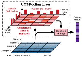
(a) The principle of our UOTP layer

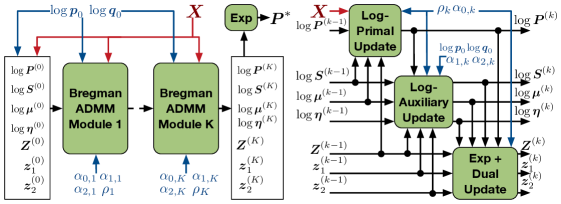
(b) The BADMM-based UOTP layer

Figure 1: (a) An illustration of the proposed UOTP layer. (b) The BADMM-based UOTP layer (left) and a single BADMM module (right). The input, model parameters, and intermediate variables are labeled in red, blue, and black. More details are shown in Section 3.1 and Appendix C.

2 Proposed UOT-Pooling Framework

2.1 A generalized formulation of global pooling operations

Denote $\mathcal{X}_{D}=\{\bm{X}\in\mathbb{R}^{D\times N}|N\in\mathbb{N}\}$ as the space of sample sets. Each $\bm{X}=[\bm{x}_{1},...,\bm{x}_{N}]\in\mathbb{R}^{D\times N}$ contains $N$ $D$-dimensional feature vectors. A global pooling operation $f:\mathcal{X}_{D}\mapsto\mathbb{R}^{D}$ maps each set to a single vector and ensures the output is permutation-invariant, $i.e.$, $f(\bm{X})=f(\bm{X}_{\pi})$ for $\bm{X},\bm{X}_{\pi}\in\mathcal{X}_{D}$, where $\bm{X}_{\pi}=[\bm{x}_{\pi(1)},...,\bm{x}_{\pi(N)}]$ and $\pi$ is an arbitrary permutation. Following the work in (Gulcehre et al., 2014; Li et al., 2020; Ko et al., 2021), we assume the input data $\bm{X}$ to be nonnegative. Note that, this assumption is reasonable in general because the input data is often processed by nonnegative activations, like ReLU, sigmoid, and so on. For some pooling methods, $e.g.$, the max-pooling shown below, the nonnegativeness is even necessary.

Typically, the widely-used mean-pooling takes the average of the input vectors as its output, $i.e.$, $f(\bm{X})=\frac{1}{N}\sum_{n=1}^{N}\bm{x}_{n}$. Another popular pooling operation, max-pooling, concatenates the maximum of each dimension as its output, $i.e.$, $f(\bm{X})=\|_{d=1}^{D}\max_{n}\{x_{dn}\}_{n=1}^{N}$, where $x_{dn}$ is the $d$-th element of $\bm{x}_{n}$ and “$\|$” represents the concatenation operator. The attention-pooling in (Ilse et al., 2018) derives a vector on the $(N-1)$-Simplex from the input $\bm{X}$ and outputs the weighted summation of the input vectors, $i.e.$, $f(\bm{X})=\bm{X}\bm{a}_{\bm{X}}$ and $\bm{a}_{\bm{X}}=\text{softmax}(\bm{w}^{T}\text{tanh}(\bm{VX}))^{T}\in\Delta^{N-1}$.

For each $\bm{X}$, its element $x_{dn}$ corresponds to a “sample-feature” pair. Essentially, the above global pooling operations would like to predict the significance of such pairs and output their weighted column-wise average. In particular, denote $\bm{P}=[p_{dn}]\in[0,1]^{D\times N}$ as the joint distribution of the sample index and the feature dimension. We obtain a generalized formulation of global pooling:

$$f(\bm{X})=(\bm{X}\odot\underbrace{\text{diag}^{-1}(\bm{P1}_{N})\bm{P}}_{\tilde{\bm{P}}=[p_{n|d}]})\bm{1}_{N}=\big{\|}_{d=1}^{D}\mathbb{E}_{n\sim p_{n|d}}[x_{dn}],$$ (1)

where $\odot$ is the Hadamard product, $\text{diag}(\cdot)$ converts a vector to a diagonal matrix, and $\bm{1}_{N}$ represents the $N$-dimensional all-one vector. $\bm{P1}_{N}=\bm{p}$ is the marginal distribution of $\bm{P}$ corresponding to feature dimensions. $\text{diag}^{-1}(\bm{p})\bm{P}=\tilde{\bm{P}}=[p_{n|d}]$ normalizes the rows of $\bm{P}$, and the $d$-th row leads to the distribution of sample indexes conditioned on the $d$-th feature dimension. Therefore, we can interpret (1) as calculating and concatenating the conditional expectation of $x_{dn}$’s for $d=1,...,D$.

Different pooling operations derive $\bm{P}$ based on different weighting mechanisms. Mean-pooling treats each element evenly, and thus, $\bm{P}=[\frac{1}{DN}]$. Max-pooling sets $\bm{P}\in\{0,\frac{1}{D}\}^{D\times N}$ and $p_{dn}=\frac{1}{D}$ if and only if $n=\arg\max_{m}\{x_{dm}\}_{m=1}^{N}$. Attention-pooling derives $\bm{P}$ as a learnable rank-one matrix, $i.e.$, $\bm{P}=\frac{1}{D}\bm{1}_{D}\bm{a}^{T}_{\bm{X}}$. All these operations set the marginal distribution $\bm{p}=\bm{P1}_{N}$ to be uniform, $i.e.$, $\bm{p}=[\frac{1}{D}]$, while let the other marginal distribution $\bm{q}=\bm{P}^{T}\bm{1}_{D}$ unconstrained.

2.2 Global pooling via solving unbalanced optimal transport problem

The above analysis implies that we can unify typical pooling operations in an interpretable algorithmic framework, in which all these operations aim at deriving the joint distribution $\bm{P}$. From the viewpoint of statistical signal processing (Turin, 1960), the input signal $\bm{X}$ is modulated by $\bm{P}$. To keep the modulated signal as informative as possible, many systems, $e.g.$, antenna arrays in telecommunication systems, keep or enlarge its expected amplitude. Following this “expectation-maximization” principle, we learn $\bm{P}$ to maximize the expectation in (1):

$$\bm{P}^{*}=\arg\sideset{}{{}_{\bm{P}\in\Pi(\bm{p},\bm{q})}}{\max}\sideset{}{{}_{d=1}^{D}}{\sum}p_{d}\mathbb{E}_{n\sim p_{n|d}}[x_{dn}]=\arg\sideset{}{{}_{\bm{P}\in\Pi(\bm{p},\bm{q})}}{\max}\underbrace{\mathbb{E}_{(d,n)\sim\bm{P}}[x_{dn}]}_{\langle\bm{X},\bm{P}\rangle},$$ (2)

where $\langle\cdot,\cdot\rangle$ represents the inner product of matrices. $\bm{p}\in\Delta^{D-1}$ and $\bm{q}\in\Delta^{N-1}$ are the distribution of feature dimension and that of sample index, respectively, which determine the marginal distributions of $\bm{P}$, $i.e.$, $\bm{P}\in\Pi(\bm{p},\bm{q})=\{\bm{P}\geq\bm{0}|\bm{P}\bm{1}_{N}=\bm{p},\bm{P}^{T}\bm{1}_{D}=\bm{q}\}$.

Through (2), we have connected the global pooling problem to computational optimal transport — (2) is an optimal transport problem (Villani, 2008), which learns the optimal joint distribution $\bm{P}^{*}$ to maximize the expectation of $x_{dn}$. Plugging $\bm{P}^{*}$ into (1) leads to a global pooling result of $\bm{X}$. Note that, achieving global pooling merely based on (2) often suffers from some limitations in practice. Firstly, solving (2) is time-consuming and always leads to sparse solutions because it is a constrained linear programming problem. A sparse $\bm{P}^{*}$ tends to filter out some weak but possibly-informative values in $\bm{X}$, which may do harm to downstream tasks. Secondly, solving (2) requires us to know the marginal distributions $\bm{p}$ and $\bm{q}$ in advance, which is either infeasible or too strict in practice.

To make the framework feasible in practice, we improve the smoothness of $\bm{P}^{*}$ and introduce two prior distributions ($i.e.$, $\bm{p}_{0}$ and $\bm{q}_{0}$) to regularize the marginals of $\bm{P}^{*}$, which leads to the following unbalanced optimal transport (UOT) problem (Benamou et al., 2015; Pham et al., 2020):

$$\begin{aligned} \bm{P}_{\text{uot}}^{*}(\bm{X};\bm{\theta})=\arg\sideset{}{{}_{\bm{P}}}{\min}\langle-\bm{X},\bm{P}\rangle+\alpha_{0}\text{R}(\bm{P})+\alpha_{1}\text{KL}(\bm{P1}_{N}|\bm{p}_{0})+\alpha_{2}\text{KL}(\bm{P}^{T}\bm{1}_{D}|\bm{q}_{0}).\end{aligned}$$ (3)

Here, $\text{R}(\bm{P})$ is a smoothness regularizer making the optimal transport problem strictly-convex, whose significance is controlled by $\alpha_{0}$. We often set the regularizer to be entropic (Cuturi, 2013), $i.e.$, $\text{R}(\bm{P})=\langle\bm{P},\log\bm{P}-\bm{1}\rangle=\sum_{d,n}p_{dn}(\log p_{dn}-1)$, or quadratic (Blondel et al., 2018), $i.e.$, $\text{R}(\bm{P})=\langle\bm{P},\bm{P}\rangle$. $\text{KL}(\bm{a}|\bm{b})=\langle\bm{a},\log\bm{a}-\log\bm{b}\rangle-\langle\bm{a}-\bm{b},\bm{1}\rangle$ represents the KL-divergence between $\bm{a}$ and $\bm{b}$. The two KL-based regularizers in (3) penalize the differences between the marginals of $\bm{P}$ and the prior distributions $\bm{p}_{0}$ and $\bm{q}_{0}$, whose significance is controlled by $\alpha_{1}$ and $\alpha_{2}$, respectively. For convenience, we use $\bm{\theta}=\{\alpha_{0},\alpha_{1},\alpha_{2},\bm{p}_{0},\bm{q}_{0}\}$ to represent the model parameters.

As shown in (3), the optimal transport $\bm{P}_{\text{uot}}^{*}$ can be viewed as a function of $\bm{X}$, whose parameters are the weights of the regularizers and the prior distributions, $i.e.$, $\bm{P}_{\text{uot}}^{*}(\bm{X};\bm{\theta})$. Plugging it into (1), we obtain the proposed UOT-Pooling operation:

$$\begin{aligned} f_{\text{uot}}(\bm{X};\alpha_{0},\alpha_{1},\alpha_{2},\bm{p}_{0},\bm{q}_{0})=(\bm{X}\odot(\text{diag}^{-1}(\bm{P}_{\text{uot}}^{*}(\bm{X};\bm{\theta})\bm{1}_{N})\bm{P}_{\text{uot}}^{*}(\bm{X};\bm{\theta})))\bm{1}_{N},\end{aligned}$$ (4)

Our UOT-Pooling satisfies the requirement of permutation-invariance under mild conditions.

Theorem 1.

The UOT-Pooling in (4) is permutation-invariant, $i.e.$, $f_{\text{uot}}(\bm{X})=f_{\text{uot}}(\bm{X}_{\pi})$ for an arbitrary permutation $\pi$, when the $\bm{q}_{0}$ in (3) is a permutation-equivariant function of $\bm{X}$.

Corollary 1.1.

The UOT-Pooling in (4) is permutation-invariant when the $\bm{q}_{0}$ in (3) is uniform, $i.e.$, $\bm{q}_{0}=\frac{1}{N}\bm{1}_{N}$ for any $\bm{X}\in\mathbb{R}^{D\times N}$.

2.3 Connecting to representative pooling operations

Our UOT-Pooling provides a unified pooling framework. In particular, we demonstrate that many existing pooling operations can be formulated as the specializations of (4) under different settings.

Proposition 1 (UOT for typical pooling operations).

Given an arbitrary $\bm{X}\in\mathbb{R}^{D\times N}$, the mean-pooling, max-pooling, and the attention-pooling with attention weights $\bm{a}_{\bm{X}}$ can be equivalently achieved by the $f_{\text{uot}}(\bm{X};\alpha_{0},\alpha_{1},\alpha_{2},\bm{p}_{0},\bm{q}_{0})$ in (4) under the following configurations:

Pooling methods	$f_{\text{uot}}(\bm{X};\alpha_{0},\alpha_{1},\alpha_{2},\bm{p}_{0},\bm{q}_{0})$
Mean-pooling	$\alpha_{0},\alpha_{1},\alpha_{2}\rightarrow\infty$, $\bm{p}_{0}=\frac{1}{D}\bm{1}_{D}$, $\bm{q}_{0}=\frac{1}{N}\bm{1}_{N}$
Max-pooling	$\alpha_{0},\alpha_{2}\rightarrow 0$, $\alpha_{1}\rightarrow\infty$, $\bm{p}_{0}=\frac{1}{D}\bm{1}_{D}$, $\bm{q}_{0}=-$
Attention-pooling	$\alpha_{0},\alpha_{1},\alpha_{2}\rightarrow\infty$, $\bm{p}_{0}=\frac{1}{D}\bm{1}_{D}$, $\bm{q}_{0}=\bm{a}_{\bm{X}}$

Here, “$\bm{q}_{0}=-$” means that $\bm{q}_{0}$ is unconstrained, and $\alpha_{1},\alpha_{2}\rightarrow\infty$ means the regularizers become strict equality constraints, rather than ignoring the optimal transport term $\langle-\bm{X},\bm{P}\rangle$.

Additionally, the combination of such UOT-Pooling operations reproduces other pooling mechanisms, such as the mixed mean-max pooling operation in (Lee et al., 2016):

$$f_{\text{mix}}(\bm{X})=\omega\text{MeanPool}(\bm{X})+(1-\omega)\text{MaxPool}(\bm{X}).$$ (5)

When $\omega\in(0,1)$ is a learnable scalar, (5) is called “Mixed mean-max pooling”. When $\omega$ is parameterized as a sigmoid function of $\bm{X}$, (5) is called “Gated mean-max pooling”. Such mixed pooling operations can be achieved by integrating three UOT-Pooling operations in a hierarchical way:

Proposition 2 (Hierarchical UOT for mixed pooling).

Given an arbitrary $\bm{X}\in\mathbb{R}^{D\times N}$, the $f_{\text{mix}}(\bm{X})$ in (5) can be equivalently implemented by $f_{\text{uot}}([f_{\text{uot}}(\bm{X};\bm{\theta}_{1}),f_{\text{uot}}(\bm{X};\bm{\theta}_{2})];\bm{\theta}_{3})$, where $\bm{\theta}_{1}=\{\infty,\infty,\infty,\frac{1}{D}\bm{1}_{D},\frac{1}{N}\bm{1}_{N}\}$, $\bm{\theta}_{2}=\{0,\infty,0,\frac{1}{D}\bm{1}_{D},-\}$, and $\bm{\theta}_{3}=\{\infty,\infty,\infty,\frac{1}{D}\bm{1}_{D},[\omega,1-\omega]^{T}\}$.

The proofs of Theorem 1, Corollary 1.1, and above Propositions are given in Appendix A.

3 Implementing Learnable UOT-Pooling Layers

Beyond reproducing existing pooling operations, we can implement the UOT-Pooling as a learnable neural network layer, whose feed-forward computation solves (3) and parameters can be learned via the backpropagation. Typically, when the smoothness regularizer is entropic, we can implement the UOTP layer based on the Sinkhorn scaling algorithm (Chizat et al., 2018; Pham et al., 2020). This algorithm solves the dual problem of (3) iteratively: $i$) Initialize dual variables as $\bm{a}^{(0)}=\bm{0}_{D}$ and $\bm{b}^{(0)}=\bm{0}_{N}$. $ii$) In the $k$-th iteration, update current dual variables $\bm{a}^{(k)}$ and $\bm{b}^{(k)}$ by

$$\begin{aligned} &\bm{T}^{(k)}=\exp(\bm{a}^{(k)}\bm{1}_{N}^{T}+\bm{1}_{D}(\bm{b}^{(k)})^{T}+{\bm{X}}/{\alpha_{0}}),\quad\bm{p}^{(k)}=\bm{T}^{(k)}\bm{1}_{N},\quad\bm{q}^{(k)}=(\bm{T}^{(k)})^{T}\bm{1}_{D},\\ &\bm{a}^{(k+1)}=\frac{\alpha_{1}(\bm{a}^{(k)}+\alpha_{0}(\log\bm{p}_{0}-\log\bm{p}^{(k)}))}{\alpha_{0}(\alpha_{0}+\alpha_{1})},\quad\bm{b}^{(k+1)}=\frac{\alpha_{2}(\bm{b}^{(k)}+\alpha_{0}(\log\bm{q}_{0}-\log\bm{q}^{(k)}))}{\alpha_{0}(\alpha_{0}+\alpha_{2})}.\end{aligned}$$ (6)

$iii$) After $K$ steps, we obtain $\bm{P}_{\text{uot}}^{*}:=\bm{T}^{(K)}$. Applying the logarithmic stabilization strategy (Chizat et al., 2018; Schmitzer, 2019), we achieve the exponentiation and scaling in (6) by “LogSumExp”.

The Sinkhorn-based UOTP layer unrolls the above iterative scheme by stacking $K$ Sinkhorn modules. Each module implements (6), which takes the dual variables as its input and updates them accordingly. The parameters include: $i$) prior distributions $\{\bm{p}_{0}\in\Delta^{D-1},\bm{q}_{0}\in\Delta^{N-1}\}$, and $ii$) module-specific weights $\{\bm{\alpha}_{i}=[\alpha_{i,k}]\in(0,\infty)^{K}\}_{i=0}^{2}$, in which $\{\alpha_{i,k}\}_{i=0}^{2}$ are parameters of the $k$-th module. As shown in (Sun et al., 2016; Amos & Kolter, 2017), introducing layer-specific parameters improves the model capacity. More details can be found at Appendix B.

Algorithm 1 UOTP${}_{\text{BADMM}}(\bm{X};\{\bm{\alpha}_{i}\}_{i=0}^{2},\bm{\rho},\bm{p}_{0},\bm{q}_{0})$

1:  Initialization: Primal and auxiliary variable $\log\bm{P}^{(0)}=\log\bm{S}^{(0)}=\log(\bm{p}_{0}\bm{q}_{0}^{T})$, $\log\bm{\mu}^{(0)}=\log\bm{p}_{0}$, $\log\bm{\eta}^{(0)}=\log\bm{q}_{0}$. Dual variables $\bm{Z}^{(0)}=\bm{0}_{D\times N}$, $\bm{z}_{1}^{(0)}=\bm{0}_{D}$, $\bm{z}_{2}^{(0)}=\bm{0}_{N}$.

2:  For $k=0,...,K-1$ ($K$ BADMM Modules)

3:   Update $\bm{P}$ by (8) (Log-primal update):  When applying the entropic regularizer, set $\bm{Y}=\log\bm{S}^{(k)}+{(\bm{X}-\bm{Z}^{(k)})}/{\rho_{k}}$,   When applying the quadratic regularizer, set $\bm{Y}=\log\bm{S}^{(k)}+{(\bm{X}-\alpha_{0,k}\bm{S}^{(k)}-\bm{Z}^{(k)})}/{\rho_{k}}$,  Update $\log\bm{P}^{(k+1)}=(\log\bm{\mu}^{(k)}-\text{LogSumExp}_{\text{col}}(\bm{Y}))\bm{1}_{N}^{T}+\bm{Y}$.

4:   Update $\bm{S},\bm{\mu},\bm{\eta}$ by (9) (Log-auxiliary update):  When applying the entropic regularizer, set $\bm{Y}={(\bm{Z}^{(k)}+\rho_{k}\log\bm{P}^{(k+1)})}{(\alpha_{0,k}+\rho_{k})}$,   When applying the quadratic regularizer, set $\bm{Y}=\log\bm{P}^{(k+1)}+{(\bm{Z}^{(k)}-\alpha_{0,k}\bm{S}^{(k+1)})}{\rho_{k}}$,   Update $\log\bm{S}^{(k+1)}=\bm{1}_{D}(\log\bm{\eta}^{(k)}-\text{LogSumExp}_{\text{row}}(\bm{Y}))^{T}+\bm{Y}$,  $\log\bm{\mu}^{(k+1)}=\frac{\rho_{k}\log\bm{\mu}^{(k)}+\alpha_{1,k}\log\bm{p}_{0}-\bm{z}_{1}^{(k)}}{\rho_{k}+\alpha_{1,k}}$,  $\log\bm{\eta}^{(k+1)}=\frac{\rho_{k}\log\bm{\eta}^{(k)}+\alpha_{2,k}\log\bm{q}_{0}-\bm{z}_{2}^{(k)}}{\rho_{k}+\alpha_{2,k}}$.

5:   Update $\bm{Z},\bm{z}_{1},\bm{z}_{2}$ (Dual update): $\bm{Z}^{(k+1)}=\bm{Z}^{(k)}+\alpha_{0,k}(\bm{P}^{(k+1)}-\bm{S}^{(k+1)})$,   $\bm{z}_{1}^{(k+1)}=\bm{z}_{1}^{(k)}+\rho_{k}(\bm{\mu}^{(k+1)}-\bm{P}^{(k+1)}\bm{1}_{N})$, $\bm{z}_{2}^{(k+1)}=\bm{z}_{2}^{(k)}+\rho_{k}(\bm{\eta}^{(k+1)}-\bm{S}^{(k+1)T}\bm{1}_{D})$.

6:  Output: $\bm{P}^{*}:=\bm{P}^{(K)}$ and apply (4) accordingly.

3.1 Proposed Bregman ADMM-based UOTP layer

The Sinkhorn-based UOTP layer is restricted to solve the entropy-regularized UOT problem and may suffer from numerical instability issues, because the Sinkhorn scaling algorithm is designed for entropic optimal transport problems and is sensitive to the weight of the entropic regularizer (Xie et al., 2020). To extend the flexibility of model design and solve the numerical problem, we develop a new UOTP layer based on the Bregman ADMM algorithm (Wang & Banerjee, 2014; Xu, 2020). Here, we rewrite (3) in an equivalent format by introducing three auxiliary variables $\bm{S}$, $\bm{\mu}$ and $\bm{\eta}$:

$$\begin{aligned} \sideset{}{{}_{\bm{P}=\bm{S},~{}\bm{P}\bm{1}_{N}=\bm{\mu},~{}\bm{S}^{T}\bm{1}_{D}=\bm{\eta}}}{\min}\langle-\bm{X},\bm{P}\rangle+\alpha_{0}\text{R}(\bm{P},\bm{S})+\alpha_{1}\text{KL}(\bm{\mu}|\bm{p}_{0})+\alpha_{2}\text{KL}(\bm{\eta}|\bm{q}_{0}).\end{aligned}$$ (7)

These three auxiliary variables correspond to the optimal transport $\bm{P}$ and its marginals. Here, the original smoothness regularizer $\text{R}(\bm{P})$ is rewritten based on the auxiliary variable $\bm{S}$. When using the entropic regularizer, we can set $\text{R}(\bm{P},\bm{S})=\langle\bm{S},\log\bm{S}-\bm{1}\rangle$. When using the quadratic regularizer, we set $\text{R}(\bm{P},\bm{S})=\langle\bm{P},\bm{S}\rangle$. This problem can be further rewritten in a Bregman-augmented Lagrangian form by introducing three dual variables $\bm{Z}$, $\bm{z}_{1}$, $\bm{z}_{2}$ for the three constraints in (7), respectively. Accordingly, we solve the UOT problem by alternating optimization: At the $k$-th iteration, we rewrite (7) in the following the Bregman-augmented Lagrangian form for $\bm{P}$ and update $\bm{P}$ by

$$\begin{aligned} \bm{P}^{(k+1)}=\arg\sideset{}{{}_{\bm{P}\in\Pi(\bm{\mu}^{(k)},\cdot)}}{\min}\langle-\bm{X},\bm{P}\rangle+\alpha_{0}\text{R}(\bm{P},\bm{S}^{(k)})+\langle\bm{Z}^{(k)},\bm{P}-\bm{S}^{(k)}\rangle+\rho\text{KL}(\bm{P}|\bm{S}^{(k)}).\end{aligned}$$ (8)

Here, $\Pi(\bm{\mu}^{(k)},\cdot)=\{\bm{P}>\bm{0}|\bm{P}\bm{1}_{N}=\bm{\mu}^{(k)}\}$ is the one-side constraint, and $\sigma_{\text{row}}$ is a row-wise softmax operation. The KL-divergence term $\text{KL}(\bm{P}|\bm{S}^{(k)})$ is the Bregman divergence. Similarly, given $\bm{P}^{(k+1)}$, we update the auxiliary variables $\bm{S}$, $\bm{\mu}$ and $\bm{\eta}$ by

$$\begin{aligned} \bm{S}^{(k+1)}&=\arg\sideset{}{{}_{\bm{S}\in\Pi(\cdot,\bm{\eta}^{(k)})}}{\min}\alpha_{0}\text{R}(\bm{P}^{(k+1)},\bm{S})+\langle\bm{Z}^{(k)},\bm{P}^{(k+1)}-\bm{S}\rangle+\rho\text{KL}(\bm{S}|\bm{P}^{(k+1)}),\\ \bm{\mu}^{(k+1)}&=\arg\sideset{}{{}_{\bm{\mu}}}{\min}\alpha_{1}\text{KL}(\bm{\mu}|\bm{p}_{0})+\langle\bm{z}_{1}^{(k)},\bm{\mu}-\bm{P}^{(k+1)}\bm{1}_{N}\rangle+\rho\text{KL}(\bm{\mu}|\bm{P}^{(k+1)}\bm{1}_{N}),\\ \bm{\eta}^{(k+1)}&=\arg\sideset{}{{}_{\bm{\eta}}}{\min}\alpha_{2}\text{KL}(\bm{\eta}|\bm{q}_{0})+\langle\bm{z}_{2}^{(k)},\bm{\eta}-(\bm{S}^{(k+1)})^{T}\bm{1}_{D}\rangle+\rho\text{KL}(\bm{\eta}|(\bm{S}^{(k+1)})^{T}\bm{1}_{D}),\end{aligned}$$ (9)

All the optimization problems in (8) and (9) have closed-form solutions. Finally, we update the dual variables as classic ADMM does. More detailed derivation is given in Appendix C.

As shown in Figure 1(b) and Algorithm 1, our BADMM-based UOTP layer implements the above BADMM algorithm by stacking $K$ feed-forward computational modules. Each module updates the primal, auxiliary, and dual variables, in which the logarithmic stabilization strategy (Chizat et al., 2018; Schmitzer, 2019) is applied. Similar to the Sinkhorn-based UOTP layer, our BADMM-based UOTP layer also owns module-specific weights of regularizers and shared prior distributions. For the module-specific weights, besides the $\{\bm{\alpha}_{i}\}_{i=0}^{2}$, the BADMM-based UOTP layer contains one more vector $\bm{\rho}=[\rho_{k}]\in(0,\infty)^{K}$, $i.e.$, the weights of the Bregman divergence terms.

3.2 Implementation details and comparisons

Reparametrization for unconstrained optimization. The above UOTP layers have constrained parameters: $\{\bm{\alpha}_{i}\}_{i=0}^{2}$ and $\bm{\rho}$ are positive, $\bm{p}_{0}\in\Delta^{D-1}$, and $\bm{q}_{0}\in\Delta^{N-1}$. We set $\{\bm{\alpha}_{i}=\text{softplus}(\bm{\beta}_{i})\}_{i=0}^{2}$ and $\bm{\rho}=\text{softplus}(\bm{\tau})$, where $\{\bm{\beta}_{i}\}_{i=0}^{2}$ and $\bm{\tau}$ are unconstrained parameters. For the prior distributions, we can either fix them as uniform distributions, $i.e.$, $\bm{p}_{0}=\frac{1}{D}\bm{1}_{D}$ and $\bm{q}_{0}=\frac{1}{N}\bm{1}_{N}$, or implement them as learnable attention modules, $i.e.$, $\bm{p}_{0}=\text{softmax}(\bm{U}\bm{X}\bm{1}_{N})$ and $\bm{q}_{0}=\text{softmax}(\bm{w}^{T}\text{tanh}(\bm{VX}))$ (Ilse et al., 2018), where $\bm{U},\bm{V}\in\mathbb{R}^{D\times D}$ and $\bm{w}\in\mathbb{R}^{D}$ are unconstrained. As a result, our UOTP layers can be learned by stochastic gradient descent.

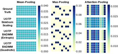
(a) Approximations of various pooling layers

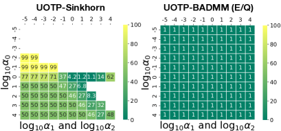
(b) Comparisons on numerical stability

Figure 2: (a) Given an arbitrary $\bm{X}\in\mathbb{R}^{5\times 10}$, we approximate the $\bm{P}^{*}$’s corresponding to the mean-, max-, and attention-pooling operations. In each subfigure, the matrices from top to bottom are the ground truth and the $\bm{P}^{*}$’s obtained by Sinkhorn-and BADMM-based UOTP layers, where $\alpha_{0}=\alpha_{1}=\alpha_{2}=10^{4}$ for mean-and attention-pooling, and $\alpha_{0}=\alpha_{2}=0.01$ and $\alpha_{1}=10^{4}$ for max-pooling. (b) Given $\bm{X}\in\mathbb{R}^{5\times 10}$, we learn $\bm{P}^{*}$’s under different configurations and calculate $\|\bm{P}^{*}\|_{1}$’s. Each subfigure shows the $\|\bm{P}^{*}\|_{1}$’s, and the white regions correspond to NaN’s. Our BADMM-based UOTP obtains the same numerical stability for both entropic and quadratic regularizers.

Precision of approximating conventional pooling methods. Proposition 1 demonstrates that our UOTP layers can approximate, even be equivalent to, some existing pooling operations. We verify this proposition by the experimental results shown in Figure 2(a). Under the configurations guided by Proposition 1, we use our UOTP layers to imitate mean-, max-, and attention-pooling operations. Both the Sinkhorn-based UOTP and the BADMM-based UOTP can reproduce the $\bm{P}^{*}$ of mean-pooling perfectly. The Sinkhorn-based UOTP achieves max-pooling with high precision, while the BADMM-based UOTP approximate max-pooling with some errors. When approximating the attention-pooling, the BADMM-based UOTP works better than the Sinkhorn-based UOTP.

Numerical stability. We set $\alpha_{1}=\alpha_{2}$ and select $\alpha_{0},\alpha_{1},\alpha_{2}$ from $\{10^{-5},...,10^{4}\}$ for for each UOTP layer. Accordingly, we derive 100 $\bm{P}^{*}$’s and check whether $\|\bm{P}^{*}\|_{1}=\sum_{d,n}|p_{dn}|\approx 1$ and whether $\bm{P}^{*}$ contains NaN elements. Figure 2(b) shows that the Sinkhorn-based UOTP merely works under some configurations. Therefore, in the following experiments, we have to restrict the range of its parameters in some cases. Our BADMM-based UOTP owns better numerical stability, which avoids NaN elements and keeps $\|\bm{P}^{*}\|_{1}\approx 1$.

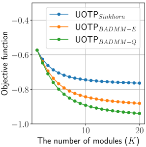
(a) Convergence comparison

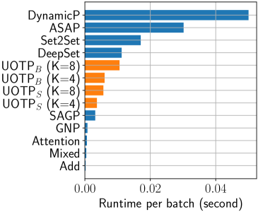
(b) Runtime comparison

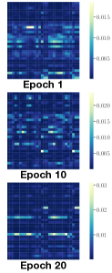
(c) Dynamics

Figure 3: Given a batch of $50$ sample sets, in which each sample set contains $500$, $100$-dimensional samples, we plot: (a) The convergence of our UOTP layers with the increase of $K$; (b) the averaged feed-forward runtime of various pooling methods in $10$ trials on a single GPU (RTX 3090). (c) Given a batch of MUTAG graphs, we illustrate dynamics of the corresponding $\bm{P}^{*}$’s during training.

Convergence and efficiency. Given $N$ $D$-dimensional samples, the computational complexity of our UOTP layer is $\mathcal{O}(KND)$, where $K$ is the number of Sinkhorn/BADMM modules. As shown in Figure 3(a), with the increase of $K$, our UOTP layers reduce the objective of the UOT problem ($i.e.$, the expectation term $\langle-\bm{X},\bm{P}\rangle$ and its regularizers) consistently. When $K\geq 4$, the objective has been reduced significantly, and when $K\geq 8$, the objective has tended to convergent.

Both the Sinkhorn-based and the BADMM-based UOTP layers involve two LogSumExp operations (the most time-consuming operations) per step. In practice, the BADMM-based UOTP may be slightly slower than the Sinkhorn-based UOTP in general — it requires additional element-wise exponentiation to get $\bm{P},\bm{S},\bm{\mu},\bm{\eta}$ when updating dual variables (Line 5 of Algorithm 1). However, the runtime of our method is comparable to that of the learning-based pooling methods. Figure 3(b) shows the rank of various pooling methods on their runtime per batch. We can find that In particular, for the BADMM-based UOTP layer with $K=8$, its runtime is almost the same with that of DeepSet (Zaheer et al., 2017). For the Sinkhorn-based UOTP layer with $K=4$, its runtime is comparable to that of SAGP (Lee et al., 2019b). When setting $K\leq 8$, our UOTP layers are more efficient than the other pooling methods that stacks multiple computational modules ($e.g.$, Set2Set (Vinyals et al., 2015) and DynamicP (Yan et al., 2018)). According to the analysis above, in the following experiments, we set $K=4$ for our UOTP layers, which can achieve a trade-off between effectiveness and efficiency in most situations.

4 Related Work

Pooling operations. Besides simple pooling operations, $e.g.$, mean/add-pooling, max-pooling, and their mixtures (Lee et al., 2016), learnable pooling layers, $e.g.$, Network-in-Network (Lin et al., 2013), Set2Set (Vinyals et al., 2015), DeepSet (Zaheer et al., 2017), and SetTransformer (Lee et al., 2019a), leverage multi-layer perceptrons, recurrent neural networks, and transformers (Vaswani et al., 2017) to achieve global pooling. The attention-pooling in (Ilse et al., 2018) and the dynamic-pooling in (Yan et al., 2018) merge multiple instances based on self-attentive mechanisms. Besides the above global pooling methods, some local pooling methods, $e.g.$, DiffPool (Ying et al., 2018), SAGPooling (Lee et al., 2019b), and ASAPooling (Ranjan et al., 2020), are proposed for pooling graph-structured data. Recently, the OTK in (Mialon et al., 2020) and the WEGL in (Kolouri et al., 2020) consider the optimal transport between samples and achieve pooling operations for specific tasks. Different from above methods, our UOTP considers the optimal transport across sample index and feature dimension, which provides a new and generalized framework of global pooling. Compared with the generalized norm-based pooling (GNP) in (Ko et al., 2021), our UOTP covers more pooling methods and can be interpreted well as an expectation-maximization strategy.

Optimal transport-based machine learning. Optimal transport (OT) theory (Villani, 2008) has proven to be useful in machine learning tasks, $e.g.$, distribution matching (Frogner et al., 2015; Courty et al., 2016), data clustering (Cuturi & Doucet, 2014), and generative modeling (Arjovsky et al., 2017; Tolstikhin et al., 2018). The discrete OT problem is a linear programming problem (Kusner et al., 2015). By adding an entropic regularizer (Cuturi, 2013), the problem becomes strictly convex and can be solved by the Sinkhorn scaling algorithm (Sinkhorn & Knopp, 1967). Along this direction, the stabilized Sinkhorn algorithm (Chizat et al., 2018; Schmitzer, 2019) and the proximal point method (Xie et al., 2020) solve the entropic OT problem robustly. These algorithms can be extended to solve UOT problems (Benamou et al., 2015; Pham et al., 2020). Recently, some neural networks are designed to imitate the Sinkhorn-based algorithms, $e.g.$, the Gumbel-Sinkhorn network (Mena et al., 2018), the sparse Sinkhorn attention model (Tay et al., 2020), the Sinkhorn autoencoder (Patrini et al., 2020), and the Sinkhorn-based transformer (Sander et al., 2021). However, these models ignore the potentials of other algorithms, $e.g.$, the Bregman ADMM (Wang & Banerjee, 2014; Xu, 2020) and the smoothed semi-dual algorithm (Blondel et al., 2018). None of them consider implementing global pooling layers as solving the UOT problem.

Table 1: Comparison on classification accuracy$\pm$Std. (%) for different pooling layers.

Pooling

Multi-instance learning

Graph classification (ADGCL)

Messidor

Component

Function

Process

NCII

PROTEINS

MUTAG

COLLAB

RDT-B

RDT-M5K

IMDB-B

IMDB-M

Add

74.33${}_{\pm\text{2.56}}$

93.35${}_{\pm\text{0.98}}$

96.26${}_{\pm\text{0.48}}$

97.41${}_{\pm\text{0.21}}$

67.96${}_{\pm\text{0.43}}$

72.97${}_{\pm\text{0.54}}$

89.05${}_{\pm\text{0.86}}$

71.06${}_{\pm\text{0.43}}$

80.00${}_{\pm\text{1.49}}$

50.16${}_{\pm\text{0.97}}$

70.18${}_{\pm\text{0.87}}$

47.56${}_{\pm\text{0.56}}$

Mean

74.42${}_{\pm\text{2.47}}$

93.32${}_{\pm\text{0.99}}$

96.28${}_{\pm\text{0.66}}$

97.20${}_{\pm\text{0.14}}$

64.82${}_{\pm\text{0.52}}$

66.09${}_{\pm\text{0.64}}$

86.53${}_{\pm\text{1.62}}$

72.35${}_{\pm\text{0.44}}$

83.62${}_{\pm\text{1.18}}$

52.44${}_{\pm\text{1.24}}$

70.34${}_{\pm\text{0.38}}$

48.65${}_{\pm\text{0.91}}$

Max

73.92${}_{\pm\text{3.00}}$

93.23${}_{\pm\text{0.76}}$

95.94${}_{\pm\text{0.48}}$

96.71${}_{\pm\text{0.40}}$

65.95${}_{\pm\text{0.76}}$

72.27${}_{\pm\text{0.33}}$

85.90${}_{\pm\text{1.68}}$

73.07${}_{\pm\text{0.57}}$

82.62${}_{\pm\text{1.25}}$

44.34${}_{\pm\text{1.93}}$

70.24${}_{\pm\text{0.54}}$

47.80${}_{\pm\text{0.54}}$

DeepSet

74.42${}_{\pm\text{2.87}}$

93.29${}_{\pm\text{0.95}}$

96.45${}_{\pm\text{0.51}}$

97.64${}_{\pm\text{0.18}}$

66.28${}_{\pm\text{0.72}}$

73.76${}_{\pm\text{0.47}}$

87.84${}_{\pm\text{0.71}}$

69.74${}_{\pm\text{0.66}}$

82.91${}_{\pm\text{1.37}}$

47.45${}_{\pm\text{0.54}}$

70.84${}_{\pm\text{0.71}}$

48.05${}_{\pm\text{0.71}}$

Mixed

73.42${}_{\pm\text{2.29}}$

93.45${}_{\pm\text{0.61}}$

96.41${}_{\pm\text{0.53}}$

96.96${}_{\pm\text{0.25}}$

66.46${}_{\pm\text{0.74}}$

72.25${}_{\pm\text{0.45}}$

87.30${}_{\pm\text{0.87}}$

73.22${}_{\pm\text{0.35}}$

84.36${}_{\pm\text{2.62}}$

46.67${}_{\pm\text{1.63}}$

71.28${}_{\pm\text{0.26}}$

48.07${}_{\pm\text{0.25}}$

GatedMixed

73.25${}_{\pm\text{2.38}}$

93.03${}_{\pm\text{1.02}}$

96.22${}_{\pm\text{0.65}}$

97.01${}_{\pm\text{0.23}}$

63.86${}_{\pm\text{0.76}}$

69.40${}_{\pm\text{1.93}}$

87.94${}_{\pm\text{1.28}}$

71.94${}_{\pm\text{0.40}}$

80.60${}_{\pm\text{3.89}}$

44.78${}_{\pm\text{4.53}}$

70.96${}_{\pm\text{0.60}}$

48.09${}_{\pm\text{0.44}}$

Set2Set

73.58${}_{\pm\text{3.74}}$

93.19${}_{\pm\text{0.95}}$

96.43${}_{\pm\text{0.56}}$

97.16${}_{\pm\text{0.25}}$

65.10${}_{\pm\text{1.12}}$

68.61${}_{\pm\text{1.44}}$

87.77${}_{\pm\text{0.86}}$

72.31${}_{\pm\text{0.73}}$

80.08${}_{\pm\text{5.72}}$

49.85${}_{\pm\text{2.77}}$

70.36${}_{\pm\text{0.85}}$

48.30${}_{\pm\text{0.54}}$

Attention

74.25${}_{\pm\text{3.67}}$

93.22${}_{\pm\text{1.02}}$

96.31${}_{\pm\text{0.66}}$

97.24${}_{\pm\text{0.16}}$

64.35${}_{\pm\text{0.61}}$

67.70${}_{\pm\text{0.95}}$

88.08${}_{\pm\text{1.22}}$

72.57${}_{\pm\text{0.41}}$

81.55${}_{\pm\text{4.39}}$

51.85${}_{\pm\text{0.66}}$

70.60${}_{\pm\text{0.38}}$

47.83${}_{\pm\text{0.78}}$

GatedAtt

73.67${}_{\pm\text{2.23}}$

93.42${}_{\pm\text{0.91}}$

96.51${}_{\pm\text{0.77}}$

97.18${}_{\pm\text{0.14}}$

64.66${}_{\pm\text{0.52}}$

68.16${}_{\pm\text{0.90}}$

86.91${}_{\pm\text{1.79}}$

72.31${}_{\pm\text{0.37}}$

82.55${}_{\pm\text{1.96}}$

51.47${}_{\pm\text{0.82}}$

70.52${}_{\pm\text{0.31}}$

48.67${}_{\pm\text{0.35}}$

DynamicP

73.16${}_{\pm\text{2.12}}$

93.26${}_{\pm\text{1.30}}$

96.47${}_{\pm\text{0.58}}$

97.03${}_{\pm\text{0.14}}$

62.11${}_{\pm\text{0.27}}$

65.86${}_{\pm\text{0.85}}$

85.40${}_{\pm\text{2.81}}$

70.78${}_{\pm\text{0.88}}$

67.51${}_{\pm\text{1.82}}$

32.11${}_{\pm\text{3.85}}$

69.84${}_{\pm\text{0.73}}$

47.59${}_{\pm\text{0.48}}$

GNP

73.54${}_{\pm\text{3.68}}$

92.86${}_{\pm\text{1.96}}$

96.10${}_{\pm\text{1.03}}$

96.03${}_{\pm\text{0.67}}$

68.20${}_{\pm\text{0.48}}$

73.44${}_{\pm\text{0.61}}$

88.37${}_{\pm\text{1.25}}$

72.80${}_{\pm\text{0.58}}$

81.93${}_{\pm\text{2.23}}$

51.80${}_{\pm\text{0.61}}$

70.34${}_{\pm\text{0.83}}$

48.85${}_{\pm\text{0.81}}$

ASAP

—

—

—

—

68.09${}_{\pm\text{0.42}}$

70.42${}_{\pm\text{1.45}}$

87.68${}_{\pm\text{1.42}}$

68.20${}_{\pm\text{2.37}}$

73.91${}_{\pm\text{1.50}}$

44.58${}_{\pm\text{0.44}}$

68.33${}_{\pm\text{2.50}}$

43.92${}_{\pm\text{1.13}}$

SAGP

—

—

—

—

67.48${}_{\pm\text{0.65}}$

72.63${}_{\pm\text{0.44}}$

87.88${}_{\pm\text{2.22}}$

70.19${}_{\pm\text{0.55}}$

74.12${}_{\pm\text{2.86}}$

46.00${}_{\pm\text{1.74}}$

70.34${}_{\pm\text{0.74}}$

47.04${}_{\pm\text{1.22}}$

UOTP${}_{\text{Sinkhorn}}$

75.42${}_{\pm\text{2.96}}$

93.29${}_{\pm\text{0.83}}$

96.62${}_{\pm\text{0.48}}$

97.08${}_{\pm\text{0.11}}$

68.27${}_{\pm\text{1.06}}$

73.10${}_{\pm\text{0.22}}$

88.84${}_{\pm\text{1.21}}$

71.20${}_{\pm\text{0.55}}$

81.54${}_{\pm\text{1.38}}$

51.00${}_{\pm\text{0.61}}$

70.74${}_{\pm\text{0.80}}$

47.87${}_{\pm\text{0.43}}$

UOTP${}_{\text{BADMM-E}}$

74.83${}_{\pm\text{2.07}}$

93.16${}_{\pm\text{1.02}}$

96.17${}_{\pm\text{0.43}}$

97.15${}_{\pm\text{0.16}}$

66.23${}_{\pm\text{0.50}}$

67.71${}_{\pm\text{1.70}}$

86.82${}_{\pm\text{2.02}}$

73.86${}_{\pm\text{0.44}}$

86.80${}_{\pm\text{1.19}}$

52.25${}_{\pm\text{0.75}}$

71.72${}_{\pm\text{0.88}}$

50.48${}_{\pm\text{0.14}}$

UOTP${}_{\text{BADMM-Q}}$

75.08${}_{\pm\text{2.06}}$

93.13${}_{\pm\text{0.94}}$

96.09${}_{\pm\text{0.46}}$

97.08${}_{\pm\text{0.17}}$

66.18${}_{\pm\text{0.76}}$

69.88${}_{\pm\text{0.87}}$

85.42${}_{\pm\text{1.10}}$

74.14${}_{\pm\text{0.24}}$

87.72${}_{\pm\text{1.03}}$

52.79${}_{\pm\text{0.60}}$

72.34${}_{\pm\text{0.50}}$

49.36${}_{\pm\text{0.52}}$

• The top-3 results of each data are bolded and the best result is in red.

5 Experiments

In principle, applying our UOTP layers can reduce the difficulty of the design and selection of global pooling — after learning based on observed data, our UOTP layers may either imitate some existing global pooling methods or lead to some new pooling layers fitting the data better. To verify this claim, we test our UOTP layers (UOTP${}_{\text{Sinkhorn}}$ and UOTP${}_{\text{BADMM-E}}$ with the entropic regularizer, and UOTP${}_{\text{BADMM-Q}}$ with the quadratic regularizer) in three tasks, $i.e.$, multi-instance learning, graph classification, and image classification. The baselines include $i)$ classic Add-Pooling, Mean-Pooling, and Max-Pooling; $ii)$ the Mixed-Pooling and the GatedMixed-Pooling in (Lee et al., 2016); $iii)$ the learnable pooling layers like DeepSet (Zaheer et al., 2017), Set2Set (Vinyals et al., 2015), DynamicP (Yan et al., 2018), GNP (Ko et al., 2021), and the Attention-Pooling and GatedAttention-Pooling in (Ilse et al., 2018); and $iv)$ SAGP (Lee et al., 2019b) and ASAP (Ranjan et al., 2020) for graph pooling. We ran our experiments on a server with two RTX3090 GPUs. Experimental results and implementation details are shown below and in Appendix D.

Multi-instance learning. We consider four MIL tasks, which correspond to a disease diagnose dataset (Messidor (Decencière et al., 2014)) and three gene ontology categorization datasets (Component, Function, and Process (Blaschke et al., 2005)). For each dataset, we learn a bag-level classifier, which embeds a bag of instances as input, merges the instances’ embeddings via pooling, and finally, predicts the bag’s label by a classifier. We use the AttentionDeepMIL in (Ilse et al., 2018), a representative bag-level classifier, as the backbone model and plug different pooling layers into it.

Graph classification. We consider eight representative graph classification datasets in the TUDataset (Morris et al., 2020), including three biochemical molecule datasets (NCII, MUTAG, and PROTEINS) and five social network datasets (COLLAB, RDT-B, RDT-M5K, IMDB-B, and IMDB-M). For each dataset, we implement the adversarial graph contrastive learning method (ADGCL) (Suresh et al., 2021), learning a graph isomorphism network (GIN) (Xu et al., 2018) to obtain graph embeddings. We apply different pooling operations to the GIN and use the learned graph embeddings to train an SVM classifier.

Table 1 presents the averaged classification accuracy and the standard deviation achieved by different methods under 5-fold cross-validation. For the multi-instance learning tasks, the performance of the UOTP layers is at least comparable to that of the baselines. For the graph classification tasks, our BADMM-based UOTP layers even achieve the best performance on five social network datasets. These results indicate that our work simplifies the design and selection of global pooling to some degree. In particular, none of the baselines perform consistently well across all the datasets, while our UOTP layers are comparable to the best baselines in most situations, whose performance is more stable and consistent. Therefore, in many learning tasks, instead of testing various global pooling methods empirically, we just need to select an algorithm ($i.e.$, Sinkhorn-scaling or Bregman ADMM) to implement the UOTP layer, which can achieve encouraging performance.

Dynamics and rationality. Take the UOTP${}_{\text{BADMM-E}}$ layer used for the MUTAG dataset as an example. For a validation batch, we visualize the dynamics of the corresponding $\bm{P}^{*}$’s in different epochs in Figure 3(c). In the beginning, the $\bm{P}^{*}$ is relatively dense because the node embeddings are not fully trained and may not be distinguishable. With the increase of epochs, the $\bm{P}^{*}$ becomes sparse and focuses more on significant sample-feature pairs. Additionally, to verify the rationality of the learned $\bm{P}^{*}$, we visualize some graphs and their $\bm{P}^{*}$’s in Figure 4. For the “V-shape” subgraphs in the two MUTAG graphs, we compare the corresponding submatrices shown in their $\bm{P}^{*}$’s. These submatrices obey the same pattern, which means that for the subgraphs shared by different samples, the weights of their node embeddings will be similar. For the key nodes in the two IMDB-B graphs, their corresponding columns in the $\bm{P}^{*}$’s are distinguished from other columns. For the nodes belonging to different communities, their columns in the $\bm{P}^{*}$’s own significant clustering structures.

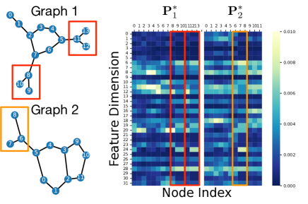
(a) MUTAG

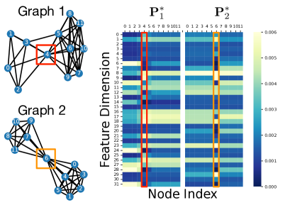
(b) IMDB-B

Figure 4: (a) The visualizations of two MUTAG graphs and their $\bm{P}^{*}$’s. For the “V-shape” subgraphs, their submatrices in the $\bm{P}^{*}$’s are marked by color frames. (b) The visualizations of two IMDB-B graphs and their $\bm{P}^{*}$’s. For each graph, its key node connecting two communities and the corresponding column in the $\bm{P}^{*}$’s are marked by color frames.

Table 2: Comparisons for ResNets and our ResNets + UOTP on validation accuracy (%)

	Learning Strategy	ResNet18	ResNet34	ResNet50	ResNet101	ResNet152
Top-5	100 Epochs (A2DP)	89.084	91.433	92.880	93.552	94.048
	90 Epochs (A2DP) + 10 Epochs (UOTP)	89.174	91.458	93.006	93.622	94.060
Top-1	100 Epochs (A2DP)	69.762	73.320	76.142	77.386	78.324
	90 Epochs (A2DP) + 10 Epochs (UOTP)	69.906	73.426	76.446	77.522	78.446

Image classification. Given a ResNet (He et al., 2016), we replace its “adaptive 2D mean-pooling layer (A2DP)” with our UOTP${}_{\text{BADMM-E}}$ layer and finetune the modified model on ImageNet (Deng et al., 2009). In particular, given the output of the last convolution layer of the ResNet, $i.e.$, $\bm{X}_{\text{in}}\in\mathbb{R}^{B\times C\times H\times W}$, our UOTP layer fuses the data and outputs $\bm{X}_{\text{out}}\in\mathbb{R}^{B\times C\times 1\times 1}$. In this experiments, we apply a two-stage learning strategy: we first train a ResNet in 90 epochs; and then we replace its A2DP layer with our UOTP layer; finally, we fix other layers and train our UOTP layer in 10 epochs. The learning rate is 0.001, and the batch size is 256. Table 2 shows that using our UOTP layer helps to improve the classification accuracy and the improvement is consistent for different ResNets.

Limitations and future work. The improvements in Table 2 are incremental because we just replace a single global pooling layer with our UOTP layer. When training the ResNets with UOTP layers from scratch, the improvements are not so significant, either — after training ResNet18+UOTP with 100 epochs, the top-1 accuracy is 69.920% and the top-5 accuracy is 89.198%. In principle, replacing more local pooling layers with our UOTP layers may bring better performance. However, given a tensor $\bm{X}_{\text{in}}\in\mathbb{R}^{B\times C\times H\times W}$, a local pooling merges each patch with size $(B\times C\times 2\times 2)$ into $B$ $C$-dimensional vectors and outputs $\bm{X}_{\text{out}}\in\mathbb{R}^{B\times C\times\frac{H}{2}\times\frac{W}{2}}$, which involves $\frac{BHW}{4}$ pooling operations. Such a local pooling requires an efficient CUDA implementation of the UOTP layers, which will be our future work.

6 Conclusion

In this work, we studied global pooling through the lens of optimal transport and demonstrated that many existing global pooling operations correspond to solving a UOT problem with different configurations. We implemented the UOTP layer based on different algorithms and analyzed their stability and complexity in details. Experiments verify their feasibility in various learning tasks.

Appendix A Delayed Proofs

A.1 Proof of Theorem 1 and Corollary 1.1

Proof.

Suppose that $\bm{q}_{0}$ be a permutation-equivariant function of $\bm{X}$, $i.e.$, $\bm{q}_{0}=g(\bm{X})$, where $g:\mathcal{X}_{D}\mapsto\Delta^{N-1}$ and $\bm{q}_{0,\pi}=g_{\pi}(\bm{X})=g(\bm{X}_{\pi})$ for an arbitrary permutation $\pi:\{1,...,N\}\mapsto\{1,....,N\}$. In such a situation, if $\bm{P}^{*}$ is the optimal solution of (3) given $\bm{X}$, then $\bm{P}^{*}_{\pi}$ must be the optimal solution of (3) given $\bm{X}_{\pi}$ because for each term in (3), we have

$$\begin{aligned} &\langle-\bm{X},\bm{P}\rangle=\langle-\bm{X}_{\pi},\bm{P}_{\pi}\rangle,\\ &\text{R}(\bm{P})=\text{R}(\bm{P}_{\pi})~{}\text{for both entropic and quadratic cases},\\ &\text{KL}(\bm{P1}_{N}|\bm{p}_{0})=\text{KL}(\bm{P}_{\pi}\bm{1}_{N}|\bm{p}_{0}),~{}\text{and}\\ &\text{KL}(\bm{P}^{T}\bm{1}_{D}|\bm{q}_{0})=\text{KL}(\bm{P}_{\pi}^{T}\bm{1}_{D}|\bm{q}_{0,\pi})=\text{KL}(\bm{P}_{\pi}^{T}\bm{1}_{D}|g(\bm{X}_{\pi})).\end{aligned}$$ (10)

As a result, $\bm{P}^{*}$ is also a permutation-equivariant function of $\bm{X}$, $i.e.$, $\bm{P}^{*}_{\pi}(\bm{X})=\bm{P}^{*}(\bm{X}_{\pi})$, and accordingly, we have

$$\begin{aligned} f_{\text{uot}}(\bm{X}_{\pi})=&(\bm{X}_{\pi}\odot(\text{diag}^{-1}(\bm{P}^{*}(\bm{X}_{\pi})\bm{1}_{N})\bm{P}^{*}(\bm{X}_{\pi})))\bm{1}_{N}\\ =&(\bm{X}_{\pi}\odot(\text{diag}^{-1}(\bm{P}_{\pi}^{*}(\bm{X})\bm{1}_{N})\bm{P}_{\pi}^{*}(\bm{X})))\bm{1}_{N}\\ =&(\bm{X}_{\pi}\odot(\text{diag}^{-1}(\bm{P}^{*}(\bm{X})\bm{1}_{N})\bm{P}_{\pi}^{*}(\bm{X})))\bm{1}_{N}\\ =&(\bm{X}\odot(\text{diag}^{-1}(\bm{P}^{*}(\bm{X})\bm{1}_{N})\bm{P}^{*}(\bm{X})))\bm{1}_{N}\\ =&f_{\text{uot}}(\bm{X}),\end{aligned}$$ (11)

which completes the proof.

Proof of Corollary 1.1: When $\bm{q}_{0}$ is uniform, we have $\text{KL}(\bm{P}^{T}\bm{1}_{D}|\bm{q}_{0})=\text{KL}(\bm{P}_{\pi}^{T}\bm{1}_{D}|\bm{q}_{0,\pi})$, which provides a special case satisfying the condition shown in Theorem 1. Accordingly, this setting also makes the optimal solution $\bm{P}^{*}$ permutation-equivariant to $\bm{X}$ and leads to the derivation in Theorem 1. ∎

A.2 Proof of Propositions 1 and 2

Proof.

Equivalence to mean-pooling: For (3), when $\alpha_{1},\alpha_{2}\rightarrow\infty$, $\bm{p}_{0}=\frac{1}{D}\bm{1}_{D}$ and $\bm{q}_{0}=\frac{1}{N}\bm{1}_{N}$, we require the marginals of $\bm{P}^{*}$ to match with $\bm{p}_{0}$ and $\bm{q}_{0}$ strictly. Additionally, $\alpha_{0}\rightarrow\infty$ means that the first term $\langle-\bm{X},\bm{P}\rangle$ becomes ignorable compared to the second term $\alpha_{0}\text{R}(\bm{P})$. Therefore, the unbalanced optimization problem in (3) degrades to the following minimization problem:

$$\bm{P}^{*}=\arg\sideset{}{{}_{\bm{P}\in\Pi(\frac{1}{D}\bm{1}_{D},\frac{1}{N}\bm{1}_{N})}}{\min}\text{R}(\bm{P}).$$ (12)

When $\text{R}(\bm{P})$ is the entropic or the quadratic regularizer, the objective function is strictly-convex, and the optimal solution is $\bm{P}^{*}=[\frac{1}{DN}]$. Therefore, the corresponding $f_{\text{uot}}$ becomes the mean-pooling operation.

Equivalence to max-pooling: For (3), when $\alpha_{0}=\alpha_{2}\rightarrow 0$, both the entropic term and the KL-based regularizer on $\bm{P}^{T}\bm{1}_{D}$ are ignorable. Additionally, $\alpha_{1}\rightarrow\infty$ and $\bm{p}_{0}=\frac{1}{D}\bm{1}_{D}$ mean that $\bm{P1}_{N}=\frac{1}{D}\bm{1}_{D}$ strictly. The problem in (3) becomes

$$\bm{P}^{*}=\arg\sideset{}{{}_{\bm{P}\in\Pi(\frac{1}{D}\bm{1}_{D},\cdot)}}{\max}\langle\bm{X},\bm{P}\rangle,$$ (13)

whose optimal solution obviously corresponds to setting $p^{*}_{dn}=\frac{1}{D}$ if and only if $n=\arg\max_{m}\{x_{dm}\}_{m=1}^{M}$. Therefore, the corresponding $f_{\text{uot}}$ becomes the max-pooling operation.

Equivalence to attention-pooling: Similar to the case of mean-pooling, under such a configuration, the problem in (3) becomes the following minimization problem:

$$\bm{P}^{*}=\arg\sideset{}{{}_{\bm{P}\in\Pi(\frac{1}{D}\bm{1}_{D},\bm{a}_{\bm{X}})}}{\max}\text{R}(\bm{P}).$$ (14)

Similar to the case of mean-pooling, when $\text{R}(\bm{P})$ is the entropic or the quadratic regularizer, the objective function is strictly-convex, and the optimal solution is $\bm{P}^{*}=\frac{1}{D}\bm{1}_{D}\bm{a}_{\bm{X}}^{T}$. Accordingly, the corresponding $f_{\text{uot}}$ becomes the self-attentive pooling operation.

Equivalence to mixed mean-max pooling: For the mixed mean-max pooling, we have

$$\begin{aligned} f_{\text{mix}}(\bm{X})&=\omega\text{MeanPool}(\bm{X})+(1-\omega)\text{MaxPool}(\bm{X})\\ &=\omega f_{\text{uot}}(\bm{X};\bm{\theta}_{1})+(1-\omega)f_{\text{uot}}(\bm{X};\bm{\theta}_{2})=\underbrace{[f_{\text{uot}}(\bm{X};\bm{\theta}_{1}),f_{\text{uot}}(\bm{X};\bm{\theta}_{2})]}_{\bm{Y}\in\mathbb{R}^{D\times 2}}[\omega,1-\omega]^{T}\\ &=\Bigl{(}\bm{Y}\odot\text{diag}^{-1}\bigl{(}\underbrace{\overbrace{\tfrac{1}{D}\bm{1}_{D}}^{\bm{p}_{0}}\overbrace{[\omega,1-\omega]}^{\bm{q}_{0}^{T}}}_{\bm{P}^{*}}\bm{1}_{2}\bigr{)}\bigl{(}\tfrac{1}{D}\bm{1}_{D}[\omega,1-\omega]\bigr{)}\Bigr{)}\bm{1}_{2}=f_{\text{uot}}(\bm{Y};\bm{\theta}_{3}).\end{aligned}$$ (15)

Here, the first equation is based on Proposition 1 — we can replace $\text{MeanPool}(\bm{X})$ and $\text{MaxPool}(\bm{X})$ with $f_{\text{uot}}(\bm{X};\bm{\theta}_{1})$ and $f_{\text{uot}}(\bm{X};\bm{\theta}_{2})$, respectively, where $\bm{\theta}_{1}=\{\infty,\infty,\infty,\frac{1}{D}\bm{1}_{D},\frac{1}{N}\bm{1}_{N}\}$ and $\bm{\theta}_{2}=\{0,\infty,0,\frac{1}{D}\bm{1}_{D},-\}$. The concatenation of $f_{\text{uot}}(\bm{X};\bm{\theta}_{1})$ and $f_{\text{uot}}(\bm{X};\bm{\theta}_{2})$ is a matrix with size $D\times 2$, denoted as $\bm{Y}$. As shown in the third equation of (15), the $f_{\text{mix}}(\bm{X})$ in (5) can be rewritten based on $\bm{p}_{0}=\frac{1}{D}\bm{1}_{D}$, $\bm{q}_{0}=[\omega,1-\omega]^{T}$, and the rank-1 matrix $\bm{P}^{*}=\bm{p}_{0}\bm{q}_{0}^{T}$. The formulation corresponds to passing $\bm{Y}$ through the third ROTP operation, $i.e.$, $f_{\text{uot}}(\bm{Y};\bm{\theta}_{3})$, where $\bm{\theta}_{3}=\{\infty,\infty,\infty,\frac{1}{D}\bm{1}_{D},[\omega,1-\omega]^{T}\}$. ∎

Appendix B The Details of Sinkhorn Scaling for UOT Problem

B.1 The dual form of UOT problem

In the case of using the entropic regularizer, given the prime form of the UOT problem in (3), we can formulate its dual form as

$$\begin{aligned} \sideset{}{{}_{\bm{a}\in\mathbb{R}^{D},\bm{b}\in\mathbb{R}^{N}}}{\min}\alpha_{0}\sideset{}{{}_{d,n=1}^{D,N}}{\sum}\exp\bigl{(}\frac{a_{d}+b_{n}+x_{dn}}{\alpha_{1}}\bigr{)}+F^{*}(-\bm{a})+G^{*}(-\bm{b}),\end{aligned}$$ (16)

where

$$\begin{aligned} F^{*}(\bm{a})&=\sideset{}{{}_{\bm{z}\in\mathbb{R}^{D}}}{\max}\bm{z}^{T}\bm{a}-\alpha_{1}\text{KL}(\bm{z}|\bm{p}_{0})=\alpha_{1}\langle\exp\bigl{(}\frac{1}{\alpha_{1}}\bm{a}\bigr{)}-\bm{1}_{D},\bm{p}_{0}\rangle.\\ G^{*}(\bm{b})&=\sideset{}{{}_{\bm{z}\in\mathbb{R}^{N}}}{\max}\bm{z}^{T}\bm{b}-\alpha_{2}\text{KL}(\bm{z}|\bm{q}_{0})=\alpha_{2}\langle\exp\bigl{(}\frac{1}{\alpha_{2}}\bm{b}\bigr{)}-\bm{1}_{N},\bm{q}_{0}\rangle.\end{aligned}$$ (17)

Plugging (17) into (16) leads to the dual form in (18):

$$\begin{aligned} \sideset{}{{}_{\bm{a}\in\mathbb{R}^{D},\bm{b}\in\mathbb{R}^{N}}}{\min}&\alpha_{0}\sideset{}{{}_{d,n=1}^{D,N}}{\sum}\exp\left(\frac{a_{d}+b_{n}+x_{dn}}{\alpha_{0}}\right)+\\ &\alpha_{1}\langle\exp(-\frac{1}{\alpha_{1}}\bm{a}),\bm{p}_{0}\rangle+\alpha_{2}\langle\exp(-\frac{1}{\alpha_{2}}\bm{b}),\bm{q}_{0}\rangle.\end{aligned}$$ (18)

This problem can be solved by the iterative steps shown in (6).

Algorithm 2 UOTP${}_{\text{Sinkhorn}}(\bm{X};\{\bm{\alpha}_{i}\}_{i=0}^{2},\bm{p}_{0},\bm{q}_{0})$

1:  Initialize $\bm{a}^{(0)}=\bm{0}_{D}$ and $\bm{b}^{(0)}=\bm{0}_{N}$, $\bm{Y}^{(0)}=\frac{1}{\alpha_{0,0}}\bm{X}$.

2:  For $k=0,...,K-1$ ($K$ Sinkhorn Modules)

3:   $\log\bm{p}=\text{LogSumExp}_{\text{col}}(\bm{Y}^{(k)})$, $\log\bm{q}=\text{LogSumExp}_{\text{row}}(\bm{Y}^{(k)})$.

4:   $\bm{a}^{(k+1)}=\frac{\alpha_{1,k}(\bm{a}^{(k)}+\alpha_{0,k}(\log\bm{p}_{0}-\log\bm{p}))}{\alpha_{0,k}(\alpha_{0,k}+\alpha_{1,k})}$, $\bm{b}^{(k+1)}=\frac{\alpha_{2,k}(\bm{b}^{(k)}+\alpha_{0,k}(\log\bm{q}_{0}-\log\bm{q}))}{\alpha_{0,k}(\alpha_{0,k}+\alpha_{2,k})}$.

5:   Logarithmic Scaling: $\bm{Y}^{(k+1)}=\frac{1}{\alpha_{0,k}}\bm{X}+\bm{a}^{(k+1)}\bm{1}_{N}^{T}+\bm{1}_{D}(\bm{b}^{(k+1)})^{T}$.

6:  Output: $\bm{P}^{*}:=\exp(\bm{Y}^{(K)})$ and apply (4) accordingly.

B.2 The implementation of the Sinkhorn-based UOTP layer

As shown in Algorithm 2, the Sinkhorn-based UOTP layer unrolls the iterative Sinkhorn scaling by stacking $K$ modules. The Sinkhorn-based UOTP layer unrolls the above iterative scheme by stacking $K$ modules. Each module implements (6), which takes the dual variables as its input and updates them accordingly.

Appendix C The Details of Bregman ADMM for UOT Problem

For the UOT problem with auxiliary variables ($i.e.$, (7)), we can write its Bregman augmented Lagrangian form as

$$\sideset{}{{}_{\bm{P},\bm{S},\bm{\mu},\bm{\eta},\bm{Z},\bm{z}_{1},\bm{z}_{2}}}{\min}\underbrace{\langle-\bm{X},\bm{P}\rangle}_{\text{OT problem}}+\underbrace{\alpha_{0}\text{R}(\bm{P},\bm{S})}_{\text{Regularizer 1}}+\underbrace{\alpha_{1}\text{KL}(\bm{\mu}|\bm{p}_{0})}_{\text{Regularizer 2}}+\underbrace{\alpha_{2}\text{KL}(\bm{\eta}|\bm{q}_{0})}_{\text{Regularizer 3}}+$$ (19)

$$\underbrace{\overbrace{\langle\bm{Z},\bm{P}-\bm{S}\rangle+\rho\text{Div}(\bm{P},\bm{S})}^{\text{Constraint 1, for $\bm{T}$ and $\bm{S}$}}+\overbrace{\langle\bm{z}_{1},\bm{\mu}-\bm{P}\bm{1}_{N}\rangle+\rho\text{Div}(\bm{\mu},\bm{P}\bm{1}_{N})}^{\text{Constraint 2, for $\bm{\mu}$ and $\bm{T}$}}+\overbrace{\langle\bm{z}_{2},\bm{\eta}-\bm{S}^{T}\bm{1}_{D}\rangle+\rho\text{Div}(\bm{\eta},\bm{S}^{T}\bm{1}_{N})}^{\text{Constraint 3, for $\bm{\eta}$ and $\bm{S}$}}}_{\text{Bregman augmented Lagrangian terms}}.$$

Here, $\text{Div}(\cdot,\cdot)$ represents the Bregman divergence term, which is implemented as the KL-divergence in this work. The second line of (19) contains the Bregman augmented Lagrangian terms, which correspond to the three constraints in (7).

At the $k$-th iteration, given current variables $\{\bm{P}^{(k)},\bm{S}^{(k)},\bm{\mu}^{(k)},\bm{\eta}^{(k)},\bm{Z}^{(k)},\bm{z}_{1}^{(k)},\bm{z}_{2}^{(k)}\}$, we update them by alternating optimization. When updating the primal variable $\bm{P}$, we can ignore Constraint 3 and the three regularizers (because they are unrelated to $\bm{P}$) and write the Constraint 2 explicitly. Then, the problem becomes:

$$\begin{aligned} &\sideset{}{{}_{\bm{P}\in\Pi(\bm{\mu}^{(k)},\cdot)}}{\min}L_{\bm{P}}\\ &=\sideset{}{{}_{\bm{P}\in\Pi(\bm{\mu}^{(k)},\cdot)}}{\min}\langle-\bm{X},\bm{P}\rangle+\alpha_{0}\text{R}(\bm{P},\bm{S}^{(k)})+\langle\bm{Z}^{(k)},\bm{P}-\bm{S}^{(k)}\rangle+\rho\underbrace{\text{Div}(\bm{P},\bm{S}^{(k)})}_{\text{KL}(\bm{P}|\bm{S}^{(k)})}.\end{aligned}$$ (20)

When using the entropic regularizer, $\text{R}(\bm{P},\bm{S}^{(k)})=\langle\bm{S}^{(k)},\log\bm{S}^{(k)}-\bm{1}\rangle$ is a constant. Applying the first-order optimality condition, we have

$$\begin{aligned} &\frac{\partial L_{\bm{P}}}{\partial\bm{P}}=\bm{0}\\ &\Rightarrow~{}~{}\rho\log\bm{P}-\bm{X}+\bm{Z}^{(k)}-\rho\log\bm{S}^{(k)}=\bm{0}\\ &\Rightarrow~{}~{}\bm{P}=\exp\left(\frac{\bm{X}-\bm{Z}^{(k)}+\rho\log\bm{S}^{(k)}}{\rho}\right)\\ &\xRightarrow{\text{Project to $\Pi(\bm{\mu}^{(k)},\cdot)$}}\bm{P}^{(k+1)}=\text{diag}(\bm{\mu}^{(k)})\sigma_{\text{row}}\left(\frac{\bm{X}-\bm{Z}^{(k)}+\rho\log\bm{S}^{(k)}}{\rho}\right)\\ &\xRightarrow{\text{Logarithmic Update}}\log\bm{P}^{(k+1)}=(\log\bm{\mu}^{(k)}-\text{LogSumExp}_{\text{col}}(\bm{Y}))\bm{1}_{N}^{T}+\bm{Y},\\ &\text{where}~{}\bm{Y}=\frac{\rho\log\bm{S}^{(k)}+\bm{X}-\bm{Z}^{(k)}}{\rho}.\end{aligned}$$ (21)

When using the quadratic regularizer, we have $\text{R}(\bm{P},\bm{S}^{(k)})=\langle\bm{P},\bm{S}^{(k)}\rangle$. We obtain the closed-form solution of $\bm{P}^{(k+1)}$ by a similar way, just computing $\bm{Y}=\frac{\rho\log\bm{S}^{(k)}+\bm{X}-\alpha_{0}\bm{S}^{(k)}-\bm{Z}^{(k)}}{\rho}$.

Similarly, when updating the auxiliary variable $\bm{S}$, we ignore the OT Problem, Constraint 2, and Regularizers 2 and 3 and write the Constraint 3 explicitly. Then, the problem becomes

$$\begin{aligned} &\sideset{}{{}_{\bm{S}\in\Pi(\cdot,\bm{\eta}^{(k)})}}{\min}L_{\bm{S}}\\ &=\sideset{}{{}_{\bm{S}\in\Pi(\cdot,\bm{\eta}^{(k)})}}{\min}\alpha_{0}\text{R}(\bm{P}^{(k+1)},\bm{S})+\langle\bm{Z}^{(k)},\bm{P}^{(k+1)}-\bm{S}\rangle+\rho\underbrace{\text{Div}(\bm{S},\bm{P}^{(k+1)})}_{\text{KL}(\bm{S}|\bm{P}^{(k+1)})}.\end{aligned}$$ (22)

When using the entropic regularizer, $\text{R}(\bm{P}^{(k+1)},\bm{S})=\langle\bm{S},\log\bm{S}-\bm{1}\rangle$. Applying the first-order optimality condition, we have

$$\begin{aligned} &\frac{\partial L_{\bm{S}}}{\partial\bm{S}}=\bm{0}\\ &\Rightarrow~{}~{}(\alpha_{0}+\rho)\log\bm{S}-\bm{Z}^{(k)}-\rho\log\bm{P}^{(k+1)}=\bm{0}\\ &\Rightarrow~{}~{}\bm{S}=\exp\left(\frac{\bm{Z}^{(k)}+\rho\log\bm{P}^{(k+1)}}{\alpha_{0}+\rho}\right)\\ &\xRightarrow{\text{Project to $\Pi(\cdot,\bm{\eta}^{(k)})$}}\bm{S}^{(k+1)}=\sigma_{\text{col}}\left(\frac{\bm{Z}^{(k)}+\rho\log\bm{P}^{(k+1)}}{\alpha_{0}+\rho}\right)\text{diag}(\bm{\eta}^{(k)})\\ &\xRightarrow{\text{Logarithmic Update}}\log\bm{S}^{(k+1)}=\bm{1}_{D}(\log\bm{\eta}^{(k)}-\text{LogSumExp}_{\text{row}}(\bm{Y}))^{T}+\bm{Y},\\ &\text{where}~{}\bm{Y}=\frac{\bm{Z}^{(k)}+\rho\log\bm{P}^{(k+1)}}{\alpha_{0}+\rho}.\end{aligned}$$ (23)

Similarly, when $\text{R}(\bm{P}^{(k+1)},\bm{S})=\langle\bm{P}^{(k+1)},\bm{S}\rangle$, we can derive $\bm{S}^{(k+1)}$ by computing $\bm{Y}=\log\bm{P}^{(k+1)}+\frac{\bm{Z}^{(k)}-\alpha_{0}\bm{S}^{(k+1)}}{\rho}$.

When updating the auxiliary variable $\bm{\mu}$, we ignore the OT Problem, Regularizers 1 and 3, Constraints 1 and 3. Then, the problem becomes

$$\begin{aligned} \sideset{}{{}_{\bm{\mu}}}{\min}L_{\bm{\mu}}=\sideset{}{{}_{\bm{\mu}}}{\min}\alpha_{1}\text{KL}(\bm{\mu}|\bm{p}_{0})+\langle\bm{z}_{1}^{(k)},\bm{\mu}-\bm{P}^{(k+1)}\bm{1}_{N}\rangle+\rho\underbrace{\text{Div}(\bm{\mu},\bm{P}^{(k+1)}\bm{1}_{N})}_{\text{KL}(\bm{\mu}|\bm{P}^{(k+1)}\bm{1}_{N})},\end{aligned}$$ (24)

where $\bm{P}^{(k+1)}\bm{1}_{N}$ actually equals to $\bm{\mu}^{(k)}$ because of the constraint in (20). Therefore, we have

$$\begin{aligned} \frac{\partial L_{\bm{\mu}}}{\partial\bm{\mu}}=\bm{0}&\Rightarrow\log\bm{\mu}=\frac{\alpha_{1}\log\bm{p}_{0}+\rho\log\bm{\mu}^{(k)}-\bm{z}_{1}^{(k)}}{\alpha_{1}+\rho}\end{aligned}$$ (25)

Similarly, when updating the auxiliary variable $\bm{\eta}$, we ignore the OT Problem, Regularizers 1 and 2, Constraints 1 and 2. Then, the problem becomes

$$\begin{aligned} \sideset{}{{}_{\bm{\eta}}}{\min}L_{\bm{\eta}}=\sideset{}{{}_{\bm{\eta}}}{\min}\alpha_{1}\text{KL}(\bm{\eta}|\bm{q}_{0})+\langle\bm{z}_{2}^{(k)},\bm{\eta}-\bm{S}^{(k+1)T}\bm{1}_{D}\rangle+\rho\underbrace{\text{Div}(\bm{\eta},\bm{S}^{(k+1)T}\bm{1}_{D})}_{\text{KL}(\bm{\eta}|\bm{S}^{(k+1)T}\bm{1}_{D})},\end{aligned}$$ (26)

where $\bm{S}^{(k+1)T}\bm{1}_{D}$ actually equals to $\bm{\eta}^{(k)}$ because of the constraint in (22). Therefore, we have

$$\begin{aligned} \frac{\partial L_{\bm{\eta}}}{\partial\bm{\eta}}=\bm{0}&\Rightarrow\log\bm{\eta}=\frac{\alpha_{2}\log\bm{q}_{0}+\rho\log\bm{\eta}^{(k)}-\bm{z}_{2}^{(k)}}{\alpha_{2}+\rho}\end{aligned}$$ (27)

Finally, the dual variables are updated based on the general rule of ADMM algorithm, $i.e.$,

$$\begin{aligned} &\bm{Z}^{(t+1)}=\bm{Z}^{(t)}+\rho(\bm{P}^{(t+1)}-\bm{S}^{(t+1)}),\\ &\bm{z}_{1}^{(t+1)}=\bm{z}_{1}^{(t)}+\rho(\bm{\mu}^{(t+1)}-\bm{P}^{(t+1)}\bm{1}_{N}),\\ &\bm{z}_{2}^{(t+1)}=\bm{z}_{2}^{(t)}+\rho(\bm{\eta}^{(t+1)}-(\bm{S}^{(t+1)})^{T}\bm{1}_{D}),\end{aligned}$$ (28)

which is also applied in (Wang & Banerjee, 2014; Ye et al., 2017; Xu, 2020).

Appendix D More Experimental Results and Implementation Details

D.1 Basic information of datasets and settings for learning backbone models

For the backbone models used in each learning task, $e.g.$, the AttentionDeepMIL in (Ilse et al., 2018) for MIL and the GIN (Xu et al., 2018) for graph embedding, we determine their hyperparameters (such as epochs, batch size, learning rate, and so on) based on the typical settings used in existing methods, $i.e.$, Attention-based deep MIL (Ilse et al., 2018) and ADGCL (Suresh et al., 2021). For the ADGCL, we connect the GIN with a linear SVM classifier. For the hyperparameters of the SVM classifier, we use the default settings shown in the code of the authors. In summary, Tables 3 and 4 show the basic information of the datasets and the settings for learning backbone models. It should be noted that all the models (associated with different pooling operations) are trained in 5 trials, and each method uses the same random seed in each trial.

Table 3: The basic information of the MIL datasets and the hyperparameters for learning

Dataset	Statistics of data							Hyperparameters
	Instance	#total	#positive	#negative	#total	Minimum	Maximum	Epochs	Batch	Learning	Weight
	dimension	bags	bags	bags	instances	bag size	bag size		size	rate	decay
Messidor	687	1200	654	546	12352	8	12	50	128	0.0005	0.005
Component	200	3130	423	2707	36894	1	53	50	128	0.0005	0.005
Function	200	5242	443	4799	55536	1	51	50	128	0.0005	0.005
Process	200	11718	757	10961	118417	1	57	50	128	0.0005	0.005

Table 4: The basic information of the graph datasets and the hyperparameters of ADGCL

Dataset	Statistics of data				Hyperparameters of ADGCL
	#Graphs	Average	Average	#Classes	Node attribute	Augmentation	Epochs	Batch	Learning
		#nodes	#edges		dimension	methods*		size	rate
NCI1	4110	29.87	32.30	2	1	LED	20	32	0.001
PROTEINS	1113	39.06	72.82	2	1	LED	20	32	0.001
MUTAG	188	17.93	19.79	2	1	LED	20	32	0.001
COLLAB	5000	74.49	2457.78	3	1	LED	100	32	0.001
RDT-B	2000	429.63	497.75	2	1	LED	150	32	0.001
RDT-M5K	4999	508.52	594.87	5	1	LED	20	32	0.001
IMDB-B	1000	19.77	96.53	2	1	LED	20	32	0.001
IMDB-M	1500	13.00	65.94	3	1	LED	20	32	0.001

• “LED” for learnable edge drop.

D.2 Settings of pooling layers

For the pooling layers used in our experiments, some of them are parametrized by attention modules, and thus, need to set hidden dimension $h$. For these pooling layers, we use their default settings shown in the corresponding references (Ilse et al., 2018; Yan et al., 2018; Lee et al., 2016). Specifically, we set $h=64$ in the MIL experiment and $h=32$ in the graph embedding experiment, respectively.

Additionally, as aforementioned, the configurations of our UOTP layers include $i$) the number of stacked modules $K$; $ii$) fixing or learning $\bm{p}_{0}$ and $\bm{q}_{0}$; $iii$) whether predefining $\alpha_{0}$ for the Sinkhorn-based UOTP for avoiding numerical instability. Table 5 lists the configurations used in our experiments. We can find that our UOTP layers are robust to their hyperparameters in most situations, which can be configured easily. In particular, in most situations, we can simply set $\bm{p}_{0}$ and $\bm{q}_{0}$ as fixed uniform distributions, $K=4$ or $8$, and make $\alpha_{0}$ unconstrained for the BADMM-based UOTP layers. In the cases that the Sinkhorn-based UOTP is unstable, we have to set $\alpha_{0}$ as a large number.

Table 5: The configurations of our UOTP layers

Task	Dataset	UOTP${}_{\text{Sinkhorn}}$				UOTP${}_{\text{BADMM-E/B}}$
		$\alpha_{0}$	$\bm{p}_{0}$	$\bm{q}_{0}$	$K$	$\alpha_{0}$	$\bm{p}_{0}$	$\bm{q}_{0}$	$K$
MIL	Messidor	—	Fixed	Fixed	4	—	Fixed	Fixed	4
	Component	—	Fixed	Fixed	4	—	Fixed	Fixed	4
	Function	—	Fixed	Fixed	4	—	Fixed	Fixed	4
	Process	—	Fixed	Fixed	4	—	Fixed	Fixed	4
	NCI1	—	Fixed	Fixed	4	—	Fixed	Fixed	4
	PROTEINS	2000	Fixed	Fixed	4	—	Fixed	Fixed	4
	MUTAG	—	Fixed	Fixed	4	—	Fixed	Fixed	4
Graph	COLLAB	$10^{10}$	Fixed	Fixed	4	—	Fixed	Fixed	4
Embedding	RDT-B	$10^{12}$	Fixed	Fixed	4	—	Fixed	Fixed	4
	RDT-M5K	$10^{10}$	Fixed	Fixed	4	—	Fixed	Fixed	4
	IMDB-B	$10^{12}$	Fixed	Fixed	4	—	Fixed	Fixed	4
	IMDB-M	$10^{11}$	Fixed	Fixed	4	—	Fixed	Fixed	4

• “—” means $\alpha_{0}$ is a learnable parameters.

D.3 More experimental results

Robustness to $K$. Our UOTP layers are simple and robust. Essentially, they only have one hyperparameter — the number of stacked modules $K$. Applying a large $K$ will lead to highly-precise solutions to (3) but take more time on both feed-forward computation and backpropagation. Fortunately, in most situations, our UOTP layers can obtain encouraging performance with small $K$’s, which achieves a good trade-off between effectiveness and efficiency. Figure 5 shows the averaged classification accuracy of different UOTP layers on the 12 datasets with respect to $K$’s. The performance of our UOTP layers is stable — when $K\in[4,8]$, the change of the averaged classification accuracy is smaller than 0.4%. This result shows the robustness to the setting of $K$.

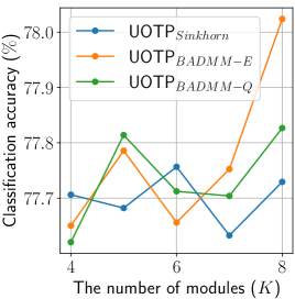
Figure 5: The averaged classification accuracy for the 12 datasets achieved by our UOTP layers under different $K$’s.

Robustness to prior distributions’ settings. Besides $K$, we also consider the settings of the prior distributions ($i.e.$, $\bm{p}_{0}$ and $\bm{q}_{0}$). As mentioned in Section 3.2, we can fix them as uniform distributions or learn them as parametric models. Take the NCI1 dataset as an example. Table 6 presents the learning results of our methods under different settings of $\bm{p}_{0}$ and $\bm{q}_{0}$. We can find that our UOT-Pooling layers are robust to their settings — the learning results do not change a lot under different settings. Therefore, in the above experiments, we fix $\bm{p}_{0}$ and $\bm{q}_{0}$ as uniform distributions. Under this simple setting, our pooling methods have already achieved encouraging results.

Table 6: The impacts of $\bm{p}_{0}$ and $\bm{q}_{0}$ on classification accuracy (%)

Layer	$\bm{p}_{0}$	$\bm{q}_{0}$	$K$	NCI1
Sinkhorn	Fixed	Fixed	4	68.27${}_{\pm\text{1.06}}$
	Learned	Fixed	4	67.97${}_{\pm\text{0.48}}$
	Fixed	Learned	4	69.86${}_{\pm\text{0.45}}$
	Learned	Learned	4	68.60${}_{\pm\text{0.15}}$
BADMM-E	Fixed	Fixed	4	66.23${}_{\pm\text{0.50}}$
	Learned	Fixed	4	65.96${}_{\pm\text{0.22}}$
	Fixed	Learned	4	66.37${}_{\pm\text{0.63}}$
	Learned	Learned	4	65.11${}_{\pm\text{0.74}}$
BADMM-Q	Fixed	Fixed	4	66.18${}_{\pm\text{0.76}}$
	Learned	Fixed	4	65.56${}_{\pm\text{0.56}}$
	Fixed	Learned	4	66.24${}_{\pm\text{0.89}}$
	Learned	Learned	4	65.40${}_{\pm\text{0.88}}$

The optimal performance achieved by grid search. The results in Table 1 are achieved by setting $K=4$ empirically. To explore the optimal performance of our method, for each dataset, we apply the grid search method to find the optimal $K$ in the range $[0,16]$, and show the results in Table 7. We can find that the results of our UOTP layers are further improved.

Table 7: Comparison on classification accuracy$\pm$Std. (%) for different pooling layers.

Pooling

Multi-instance learning

Graph classification (ADGCL)

Messidor

Component

Function

Process

NCII

PROTEINS

MUTAG

COLLAB

RDT-B

RDT-M5K

IMDB-B

IMDB-M

Add

74.33${}_{\pm\text{2.56}}$

93.35${}_{\pm\text{0.98}}$

96.26${}_{\pm\text{0.48}}$

97.41${}_{\pm\text{0.21}}$

67.96${}_{\pm\text{0.43}}$

72.97${}_{\pm\text{0.54}}$

89.05${}_{\pm\text{0.86}}$

71.06${}_{\pm\text{0.43}}$

80.00${}_{\pm\text{1.49}}$

50.16${}_{\pm\text{0.97}}$

70.18${}_{\pm\text{0.87}}$

47.56${}_{\pm\text{0.56}}$

Mean

74.42${}_{\pm\text{2.47}}$

93.32${}_{\pm\text{0.99}}$

96.28${}_{\pm\text{0.66}}$

97.20${}_{\pm\text{0.14}}$

64.82${}_{\pm\text{0.52}}$

66.09${}_{\pm\text{0.64}}$

86.53${}_{\pm\text{1.62}}$

72.35${}_{\pm\text{0.44}}$

83.62${}_{\pm\text{1.18}}$

52.44${}_{\pm\text{1.24}}$

70.34${}_{\pm\text{0.38}}$

48.65${}_{\pm\text{0.91}}$

Max

73.92${}_{\pm\text{3.00}}$

93.23${}_{\pm\text{0.76}}$

95.94${}_{\pm\text{0.48}}$

96.71${}_{\pm\text{0.40}}$

65.95${}_{\pm\text{0.76}}$

72.27${}_{\pm\text{0.33}}$

85.90${}_{\pm\text{1.68}}$

73.07${}_{\pm\text{0.57}}$

82.62${}_{\pm\text{1.25}}$

44.34${}_{\pm\text{1.93}}$

70.24${}_{\pm\text{0.54}}$

47.80${}_{\pm\text{0.54}}$

DeepSet

74.42${}_{\pm\text{2.87}}$

93.29${}_{\pm\text{0.95}}$

96.45${}_{\pm\text{0.51}}$

97.64${}_{\pm\text{0.18}}$

66.28${}_{\pm\text{0.72}}$

73.76${}_{\pm\text{0.47}}$

87.84${}_{\pm\text{0.71}}$

69.74${}_{\pm\text{0.66}}$

82.91${}_{\pm\text{1.37}}$

47.45${}_{\pm\text{0.54}}$

70.84${}_{\pm\text{0.71}}$

48.05${}_{\pm\text{0.71}}$

Mixed

73.42${}_{\pm\text{2.29}}$

93.45${}_{\pm\text{0.61}}$

96.41${}_{\pm\text{0.53}}$

96.96${}_{\pm\text{0.25}}$

66.46${}_{\pm\text{0.74}}$

72.25${}_{\pm\text{0.45}}$

87.30${}_{\pm\text{0.87}}$

73.22${}_{\pm\text{0.35}}$

84.36${}_{\pm\text{2.62}}$

46.67${}_{\pm\text{1.63}}$

71.28${}_{\pm\text{0.26}}$

48.07${}_{\pm\text{0.25}}$

GatedMixed

73.25${}_{\pm\text{2.38}}$

93.03${}_{\pm\text{1.02}}$

96.22${}_{\pm\text{0.65}}$

97.01${}_{\pm\text{0.23}}$

63.86${}_{\pm\text{0.76}}$

69.40${}_{\pm\text{1.93}}$

87.94${}_{\pm\text{1.28}}$

71.94${}_{\pm\text{0.40}}$

80.60${}_{\pm\text{3.89}}$

44.78${}_{\pm\text{4.53}}$

70.96${}_{\pm\text{0.60}}$

48.09${}_{\pm\text{0.44}}$

Set2Set

73.58${}_{\pm\text{3.74}}$

93.19${}_{\pm\text{0.95}}$

96.43${}_{\pm\text{0.56}}$

97.16${}_{\pm\text{0.25}}$

65.10${}_{\pm\text{1.12}}$

68.61${}_{\pm\text{1.44}}$

87.77${}_{\pm\text{0.86}}$

72.31${}_{\pm\text{0.73}}$

80.08${}_{\pm\text{5.72}}$

49.85${}_{\pm\text{2.77}}$

70.36${}_{\pm\text{0.85}}$

48.30${}_{\pm\text{0.54}}$

Attention

74.25${}_{\pm\text{3.67}}$

93.22${}_{\pm\text{1.02}}$

96.31${}_{\pm\text{0.66}}$

97.24${}_{\pm\text{0.16}}$

64.35${}_{\pm\text{0.61}}$

67.70${}_{\pm\text{0.95}}$

88.08${}_{\pm\text{1.22}}$

72.57${}_{\pm\text{0.41}}$

81.55${}_{\pm\text{4.39}}$

51.85${}_{\pm\text{0.66}}$

70.60${}_{\pm\text{0.38}}$

47.83${}_{\pm\text{0.78}}$

GatedAtt

73.67${}_{\pm\text{2.23}}$

93.42${}_{\pm\text{0.91}}$

96.51${}_{\pm\text{0.77}}$

97.18${}_{\pm\text{0.14}}$

64.66${}_{\pm\text{0.52}}$

68.16${}_{\pm\text{0.90}}$

86.91${}_{\pm\text{1.79}}$

72.31${}_{\pm\text{0.37}}$

82.55${}_{\pm\text{1.96}}$

51.47${}_{\pm\text{0.82}}$

70.52${}_{\pm\text{0.31}}$

48.67${}_{\pm\text{0.35}}$

DynamicP

73.16${}_{\pm\text{2.12}}$

93.26${}_{\pm\text{1.30}}$

96.47${}_{\pm\text{0.58}}$

97.03${}_{\pm\text{0.14}}$

62.11${}_{\pm\text{0.27}}$

65.86${}_{\pm\text{0.85}}$

85.40${}_{\pm\text{2.81}}$

70.78${}_{\pm\text{0.88}}$

67.51${}_{\pm\text{1.82}}$

32.11${}_{\pm\text{3.85}}$

69.84${}_{\pm\text{0.73}}$

47.59${}_{\pm\text{0.48}}$

GNP

73.54${}_{\pm\text{3.68}}$

92.86${}_{\pm\text{1.96}}$

96.10${}_{\pm\text{1.03}}$

96.03${}_{\pm\text{0.67}}$

68.20${}_{\pm\text{0.48}}$

73.44${}_{\pm\text{0.61}}$

88.37${}_{\pm\text{1.25}}$

72.80${}_{\pm\text{0.58}}$

81.93${}_{\pm\text{2.23}}$

51.80${}_{\pm\text{0.61}}$

70.34${}_{\pm\text{0.83}}$

48.85${}_{\pm\text{0.81}}$

ASAP

—

—

—

—

68.09${}_{\pm\text{0.42}}$

70.42${}_{\pm\text{1.45}}$

87.68${}_{\pm\text{1.42}}$

68.20${}_{\pm\text{2.37}}$

73.91${}_{\pm\text{1.50}}$

44.58${}_{\pm\text{0.44}}$

68.33${}_{\pm\text{2.50}}$

43.92${}_{\pm\text{1.13}}$

SAGP

—

—

—

—

67.48${}_{\pm\text{0.65}}$

72.63${}_{\pm\text{0.44}}$

87.88${}_{\pm\text{2.22}}$

70.19${}_{\pm\text{0.55}}$

74.12${}_{\pm\text{2.86}}$

46.00${}_{\pm\text{1.74}}$

70.34${}_{\pm\text{0.74}}$

47.04${}_{\pm\text{1.22}}$

UOTP${}_{\text{Sinkhorn}}$

($K=16$)

($K=10$)

($K=4$)

($K=10$)

($K=8$)

($K=8$)

($K=4$)

($K=4$)

($K=4$)

($K=8$)

($K=4$)

($K=8$)

75.92${}_{\pm\text{2.39}}$

93.67${}_{\pm\text{0.80}}$

96.62${}_{\pm\text{0.48}}$

97.18${}_{\pm\text{0.15}}$

68.44${}_{\pm\text{0.50}}$

73.36${}_{\pm\text{0.71}}$

88.84${}_{\pm\text{1.21}}$

71.20${}_{\pm\text{0.55}}$

81.54${}_{\pm\text{1.38}}$

52.04${}_{\pm\text{1.06}}$

70.74${}_{\pm\text{0.80}}$

47.95${}_{\pm\text{0.52}}$

UOTP${}_{\text{BADMM-E}}$

($K=14$)

($K=13$)

($K=16$)

($K=4$)

($K=8$)

($K=8$)

($K=7$)

($K=4$)

($K=4$)

($K=8$)

($K=8$)

($K=4$)

75.75${}_{\pm\text{2.00}}$

93.39${}_{\pm\text{0.72}}$

96.45${}_{\pm\text{0.52}}$

97.15${}_{\pm\text{0.16}}$

66.41${}_{\pm\text{0.73}}$

70.55${}_{\pm\text{1.06}}$

88.95${}_{\pm\text{1.01}}$

73.86${}_{\pm\text{0.44}}$

86.80${}_{\pm\text{1.19}}$

52.81${}_{\pm\text{0.79}}$

72.56${}_{\pm\text{0.51}}$

50.48${}_{\pm\text{0.14}}$

UOTP${}_{\text{BADMM-Q}}$

($K=11$)

($K=16$)

($K=8$)

($K=4$)

($K=4$)

($K=14$)

($K=5$)

($K=4$)

($K=8$)

($K=4$)

($K=4$)

($K=8$)

75.50${}_{\pm\text{2.29}}$

93.35${}_{\pm\text{0.83}}$

96.34${}_{\pm\text{0.56}}$

97.08${}_{\pm\text{0.17}}$

66.18${}_{\pm\text{0.76}}$

71.77${}_{\pm\text{0.85}}$

87.92${}_{\pm\text{1.11}}$

74.14${}_{\pm\text{0.24}}$

88.81${}_{\pm\text{0.79}}$

52.79${}_{\pm\text{0.60}}$

72.34${}_{\pm\text{0.50}}$

49.81${}_{\pm\text{0.64}}$

• The top-3 results of each data are bolded and the best result is in red.

References

- Amos & Kolter (2017) Brandon Amos and J Zico Kolter. Optnet: Differentiable optimization as a layer in neural networks. In International Conference on Machine Learning, pp. 136–145. PMLR, 2017.
- Arjovsky et al. (2017) Martin Arjovsky, Soumith Chintala, and Léon Bottou. Wasserstein generative adversarial networks. In International conference on machine learning, pp. 214–223. PMLR, 2017.
- Benamou et al. (2015) Jean-David Benamou, Guillaume Carlier, Marco Cuturi, Luca Nenna, and Gabriel Peyré. Iterative bregman projections for regularized transportation problems. SIAM Journal on Scientific Computing, 37(2):A1111–A1138, 2015.
- Blaschke et al. (2005) Christian Blaschke, Eduardo Andres Leon, Martin Krallinger, and Alfonso Valencia. Evaluation of biocreative assessment of task 2. BMC bioinformatics, 6(1):1–13, 2005.
- Blondel et al. (2018) Mathieu Blondel, Vivien Seguy, and Antoine Rolet. Smooth and sparse optimal transport. In International Conference on Artificial Intelligence and Statistics, pp. 880–889. PMLR, 2018.
- Boureau et al. (2010) Y-Lan Boureau, Jean Ponce, and Yann LeCun. A theoretical analysis of feature pooling in visual recognition. In International conference on machine learning, pp. 111–118, 2010.
- Chizat et al. (2018) Lenaic Chizat, Gabriel Peyré, Bernhard Schmitzer, and François-Xavier Vialard. Scaling algorithms for unbalanced optimal transport problems. Mathematics of Computation, 87(314):2563–2609, 2018.
- Courty et al. (2016) Nicolas Courty, Rémi Flamary, Devis Tuia, and Alain Rakotomamonjy. Optimal transport for domain adaptation. IEEE transactions on pattern analysis and machine intelligence, 39(9):1853–1865, 2016.
- Cuturi (2013) Marco Cuturi. Sinkhorn distances: Lightspeed computation of optimal transport. In Advances in neural information processing systems, pp. 2292–2300, 2013.
- Cuturi & Doucet (2014) Marco Cuturi and Arnaud Doucet. Fast computation of wasserstein barycenters. 2014.
- Decencière et al. (2014) Etienne Decencière, Xiwei Zhang, Guy Cazuguel, Bruno Lay, Béatrice Cochener, Caroline Trone, Philippe Gain, Richard Ordonez, Pascale Massin, Ali Erginay, et al. Feedback on a publicly distributed image database: the messidor database. Image Analysis & Stereology, 33(3):231–234, 2014.
- Deng et al. (2009) Jia Deng, R. Socher, Li Fei-Fei, Wei Dong, Kai Li, and Li-Jia Li. Imagenet: A large-scale hierarchical image database. In IEEE Conference on Computer Vision and Pattern Recognition (CVPR), pp. 248–255, 2009.
- Frogner et al. (2015) Charlie Frogner, Chiyuan Zhang, Hossein Mobahi, Mauricio Araya-Polo, and Tomaso Poggio. Learning with a wasserstein loss. In Proceedings of the 28th International Conference on Neural Information Processing Systems-Volume 2, pp. 2053–2061, 2015.
- Gulcehre et al. (2014) Caglar Gulcehre, Kyunghyun Cho, Razvan Pascanu, and Yoshua Bengio. Learned-norm pooling for deep feedforward and recurrent neural networks. In Joint European Conference on Machine Learning and Knowledge Discovery in Databases, pp. 530–546. Springer, 2014.
- He et al. (2016) Kaiming He, Xiangyu Zhang, Shaoqing Ren, and Jian Sun. Deep residual learning for image recognition. In Proceedings of the IEEE conference on computer vision and pattern recognition, pp. 770–778, 2016.
- Ilse et al. (2018) Maximilian Ilse, Jakub Tomczak, and Max Welling. Attention-based deep multiple instance learning. In International conference on machine learning, pp. 2127–2136. PMLR, 2018.
- Ko et al. (2021) Jihoon Ko, Taehyung Kwon, Kijung Shin, and Juho Lee. Learning to pool in graph neural networks for extrapolation. arXiv preprint arXiv:2106.06210, 2021.
- Kolouri et al. (2020) Soheil Kolouri, Navid Naderializadeh, Gustavo K Rohde, and Heiko Hoffmann. Wasserstein embedding for graph learning. In International Conference on Learning Representations, 2020.
- Krizhevsky et al. (2012) Alex Krizhevsky, Ilya Sutskever, and Geoffrey E Hinton. Imagenet classification with deep convolutional neural networks. Advances in neural information processing systems, 25:1097–1105, 2012.
- Kusner et al. (2015) Matt Kusner, Yu Sun, Nicholas Kolkin, and Kilian Weinberger. From word embeddings to document distances. In International conference on machine learning, pp. 957–966. PMLR, 2015.
- Lee et al. (2016) Chen-Yu Lee, Patrick W Gallagher, and Zhuowen Tu. Generalizing pooling functions in convolutional neural networks: Mixed, gated, and tree. In Artificial intelligence and statistics, pp. 464–472. PMLR, 2016.
- Lee et al. (2019a) Juho Lee, Yoonho Lee, Jungtaek Kim, Adam Kosiorek, Seungjin Choi, and Yee Whye Teh. Set transformer: A framework for attention-based permutation-invariant neural networks. In International Conference on Machine Learning, pp. 3744–3753. PMLR, 2019a.
- Lee et al. (2019b) Junhyun Lee, Inyeop Lee, and Jaewoo Kang. Self-attention graph pooling. In International Conference on Machine Learning, pp. 3734–3743. PMLR, 2019b.
- Li et al. (2020) Guohao Li, Chenxin Xiong, Ali Thabet, and Bernard Ghanem. Deepergcn: All you need to train deeper gcns. arXiv preprint arXiv:2006.07739, 2020.
- Lin et al. (2013) Min Lin, Qiang Chen, and Shuicheng Yan. Network in network. arXiv preprint arXiv:1312.4400, 2013.
- Mena et al. (2018) Gonzalo Mena, David Belanger, Scott Linderman, and Jasper Snoek. Learning latent permutations with gumbel-sinkhorn networks. In International Conference on Learning Representations, 2018.
- Mialon et al. (2020) Grégoire Mialon, Dexiong Chen, Alexandre d’Aspremont, and Julien Mairal. A trainable optimal transport embedding for feature aggregation. In International Conference on Learning Representations (ICLR), 2020.
- Morris et al. (2020) Christopher Morris, Nils M. Kriege, Franka Bause, Kristian Kersting, Petra Mutzel, and Marion Neumann. Tudataset: A collection of benchmark datasets for learning with graphs. In ICML 2020 Workshop on Graph Representation Learning and Beyond (GRL+ 2020), 2020. URL www.graphlearning.io.
- Patrini et al. (2020) Giorgio Patrini, Rianne van den Berg, Patrick Forre, Marcello Carioni, Samarth Bhargav, Max Welling, Tim Genewein, and Frank Nielsen. Sinkhorn autoencoders. In Uncertainty in Artificial Intelligence, pp. 733–743. PMLR, 2020.
- Pham et al. (2020) Khiem Pham, Khang Le, Nhat Ho, Tung Pham, and Hung Bui. On unbalanced optimal transport: An analysis of sinkhorn algorithm. In International Conference on Machine Learning, pp. 7673–7682. PMLR, 2020.
- Ranjan et al. (2020) Ekagra Ranjan, Soumya Sanyal, and Partha Talukdar. Asap: Adaptive structure aware pooling for learning hierarchical graph representations. In Proceedings of the AAAI Conference on Artificial Intelligence, volume 34, pp. 5470–5477, 2020.
- Sander et al. (2021) Michael E Sander, Pierre Ablin, Mathieu Blondel, and Gabriel Peyré. Sinkformers: Transformers with doubly stochastic attention. arXiv preprint arXiv:2110.11773, 2021.
- Schmitzer (2019) Bernhard Schmitzer. Stabilized sparse scaling algorithms for entropy regularized transport problems. SIAM Journal on Scientific Computing, 41(3):A1443–A1481, 2019.
- Sinkhorn & Knopp (1967) Richard Sinkhorn and Paul Knopp. Concerning nonnegative matrices and doubly stochastic matrices. Pacific Journal of Mathematics, 21(2):343–348, 1967.
- Sun et al. (2016) Jian Sun, Huibin Li, Zongben Xu, et al. Deep admm-net for compressive sensing mri. Advances in neural information processing systems, 29, 2016.
- Suresh et al. (2021) Susheel Suresh, Pan Li, Cong Hao, and Jennifer Neville. Adversarial graph augmentation to improve graph contrastive learning. arXiv preprint arXiv:2106.05819, 2021.
- Tay et al. (2020) Yi Tay, Dara Bahri, Liu Yang, Donald Metzler, and Da-Cheng Juan. Sparse sinkhorn attention. In International Conference on Machine Learning, pp. 9438–9447. PMLR, 2020.
- Tolstikhin et al. (2018) Ilya Tolstikhin, Olivier Bousquet, Sylvain Gelly, and Bernhard Schoelkopf. Wasserstein auto-encoders. In International Conference on Learning Representations, 2018.
- Turin (1960) George Turin. An introduction to matched filters. IRE transactions on Information theory, 6(3):311–329, 1960.
- Vaswani et al. (2017) Ashish Vaswani, Noam Shazeer, Niki Parmar, Jakob Uszkoreit, Llion Jones, Aidan N Gomez, Łukasz Kaiser, and Illia Polosukhin. Attention is all you need. In Advances in neural information processing systems, pp. 5998–6008, 2017.
- Villani (2008) Cédric Villani. Optimal transport: old and new, volume 338. Springer Science & Business Media, 2008.
- Vinyals et al. (2015) Oriol Vinyals, Samy Bengio, and Manjunath Kudlur. Order matters: Sequence to sequence for sets. arXiv preprint arXiv:1511.06391, 2015.
- Wang & Banerjee (2014) Huahua Wang and Arindam Banerjee. Bregman alternating direction method of multipliers. In Proceedings of the 27th International Conference on Neural Information Processing Systems-Volume 2, pp. 2816–2824, 2014.
- Xie et al. (2020) Yujia Xie, Xiangfeng Wang, Ruijia Wang, and Hongyuan Zha. A fast proximal point method for computing exact wasserstein distance. In Uncertainty in Artificial Intelligence, pp. 433–453. PMLR, 2020.
- Xu (2020) Hongteng Xu. Gromov-wasserstein factorization models for graph clustering. Proceedings of the AAAI Conference on Artificial Intelligence, 34(04):6478–6485, 2020.
- Xu et al. (2018) Keyulu Xu, Weihua Hu, Jure Leskovec, and Stefanie Jegelka. How powerful are graph neural networks? In International Conference on Learning Representations, 2018.
- Yan et al. (2018) Yongluan Yan, Xinggang Wang, Xiaojie Guo, Jiemin Fang, Wenyu Liu, and Junzhou Huang. Deep multi-instance learning with dynamic pooling. In Asian Conference on Machine Learning, pp. 662–677. PMLR, 2018.
- Ye et al. (2017) Jianbo Ye, Panruo Wu, James Z Wang, and Jia Li. Fast discrete distribution clustering using wasserstein barycenter with sparse support. IEEE Transactions on Signal Processing, 65(9):2317–2332, 2017.
- Ying et al. (2018) Rex Ying, Jiaxuan You, Christopher Morris, Xiang Ren, William L Hamilton, and Jure Leskovec. Hierarchical graph representation learning with differentiable pooling. In Proceedings of the 32nd International Conference on Neural Information Processing Systems, pp. 4805–4815, 2018.
- Zaheer et al. (2017) Manzil Zaheer, Satwik Kottur, Siamak Ravanbhakhsh, Barnabás Póczos, Ruslan Salakhutdinov, and Alexander J Smola. Deep sets. In Proceedings of the 31st International Conference on Neural Information Processing Systems, pp. 3394–3404, 2017.