pvCNN: Privacy-Preserving and Verifiable Convolutional Neural Network Testing

Abstract

We propose a new approach for privacy-preserving and verifiable convolutional neural network (CNN) testing in a distrustful multi-stakeholder environment. The approach is aimed to enable that a CNN model developer convinces a user of the truthful CNN performance over non-public data from multiple testers, while respecting model and data privacy. To balance the security and efficiency issues, we appropriately integrate three tools with the CNN testing, including collaborative inference, homomorphic encryption (HE) and zero-knowledge succinct non-interactive argument of knowledge (zk-SNARK).

We start with strategically partitioning a CNN model into a private part kept locally by the model developer, and a public part outsourced to an outside server. Then, the private part runs over the HE-protected test data sent by a tester, and transmits its outputs to the public part for accomplishing subsequent computations of the CNN testing. Second, the correctness of the above CNN testing is enforced by generating zk-SNARK based proofs, with an emphasis on optimizing proving overhead for two-dimensional (2-D) convolution operations, since the operations dominate the performance bottleneck during generating proofs. We specifically present a new quadratic matrix program (QMP)-based arithmetic circuit with a single multiplication gate for expressing 2-D convolution operations between multiple filters and inputs in a batch manner. Third, we aggregate multiple proofs with respect to a same CNN model but different testers’ test data (i.e., different statements) into one proof, and ensure that the validity of the aggregated proof implies the validity of the original multiple proofs. Lastly, our experimental results demonstrate that our QMP-based zk-SNARK performs nearly $13.9\times$ faster than the existing quadratic arithmetic program (QAP)-based zk-SNARK in proving time, and $17.6\times$ faster in Setup time, for high-dimension matrix multiplication. Besides, the limitation on handling a bounded number of multiplications of QAP-based zk-SNARK is relieved.

I INTRODUCTION

Convolutional neural networks (CNNs) [1, 2] have been widely applied in various application scenarios, such as healthcare analysis, autonomous vehicle and face recognition. But real-life reports demonstrate that neural networks often exhibit erroneous decisions, leading to disastrous consequences, e.g., self-driving crash due to the failure of identifying unexpected driving environments [3], and prejudice due to racial biases embedded in face recognition systems [4]. The reports emphasize that when applying CNN models in security-critical scenarios, model users should be sufficiently cautious of benchmarking the CNN models to obtain the truthful multi-faceted performance, like robustness and fairness, not limited to natural accuracy. For example, when a CNN model is deployed in a self-driving car for identifying camera images, a user should be assured that the CNN model is always highly accurate, even for perturbed images; for face recognition applications, users want to know that the underlying CNN models can accurately recognize face images without discrimination.

A widely adopted approach to benchmarking a CNN model is black-box testing [5, 6]. Black-box testing enables users to have a black-box access to the CNN model, that is, feeding the model with a batch of test data and merely observing its outputs, e.g., the proportion of correct predictions. Such approach is suitable for the setting where model users and model developers are not the same entities. The main reasons are that the parameters of CNN models are intellectual properties and are vulnerable to privacy attacks, such that developers are unwilling to reveal the parameters. We are also aware that existing excellent white-box testing approaches[7] can test CNN models in a fine-granularity fashion using model parameters, but black-box testing is preferred in the above setting where model parameters are inaccessible.

Starting by black-box testing, two essential issues need consideration to probe a CNN model’s truthful and multi-faceted performance. (i) Black-box testing strongly relies on the test dataset[7], which in turn requires multi-source data support in reality. In order to support testing a model’s multi-faceted performance, the available test dataset should be as various as possible. One evidence is that multiple benchmarks are built by embedding dozens of types of noises into ImageNet to measure the robustness of CNN models[8]. Despite the necessity, building such benchmarks consumes many manpower and multi-party efforts, even for large companies, e.g., a recent project named Crowdsourcing Adverse Test Sets for Machine Learning (CATS4ML) launched by Google Research [9]. Thus, the off-the-shelf test datasets for supporting multi-faceted CNN testing are likely from multiple sources. (ii) Black-box testing opens a door for untrusted model developers to cheat in testing. They might forge untruthful outputs without correctly running the processes of CNN testing on given test datasets. Additionally, if developers can in advance learn a given test dataset, they might craft a CNN which typically adapts to the test dataset, which deviates from our initial goal of testing their truthful multi-faceted performance. From this point, test datasets cannot be public, not merely due to that datasets themselves are privacy-sensitive in many security-critical scenarios. Motivated by the two issues above, there needs an approach for users to validate the correctness of the black-box CNN testing over multi-source test datasets, in which test datasets are not public and the CNN model is privacy-preserving.

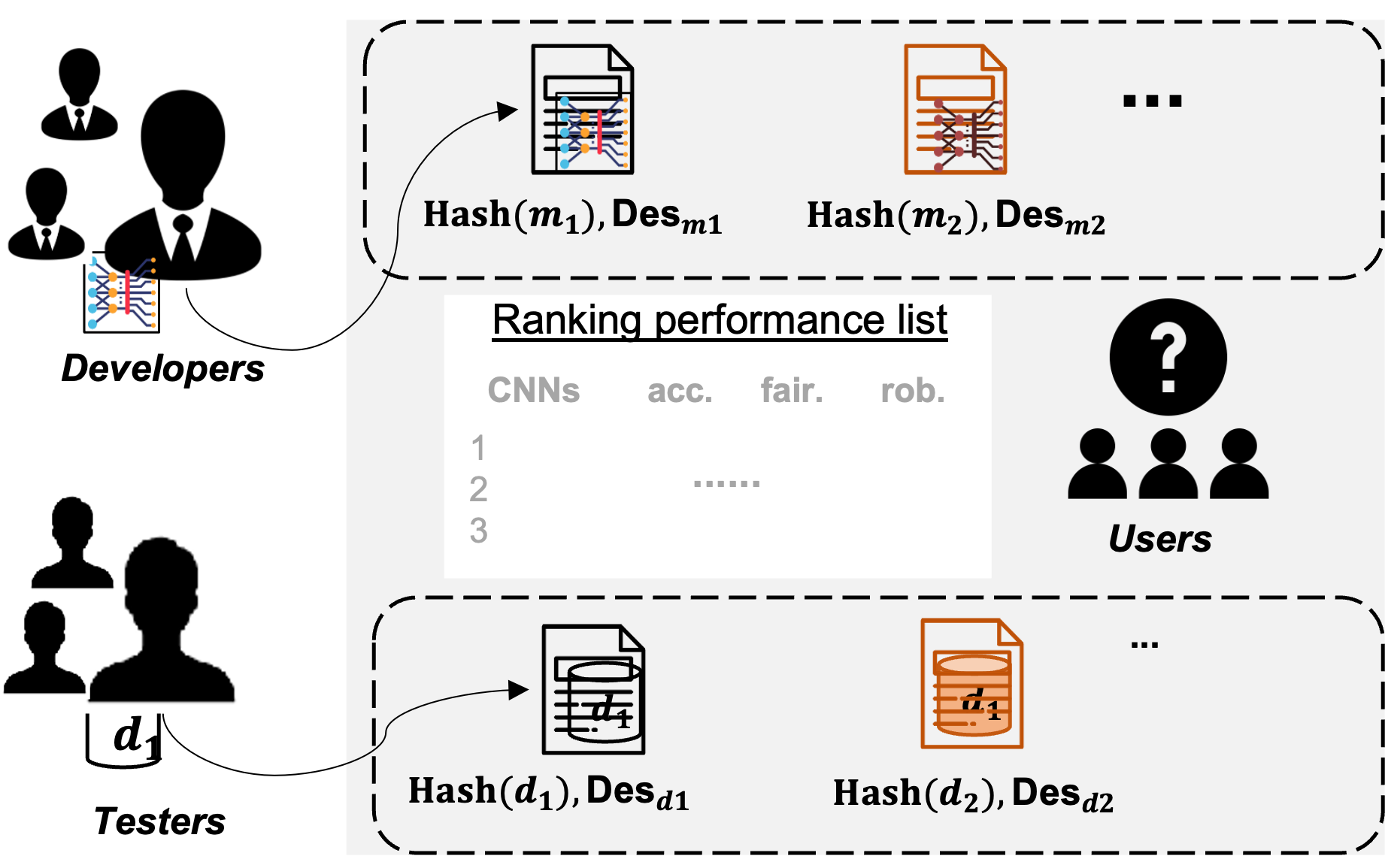
Figure 1: Scenario example ($m_{1},m_{2}$ refer to CNN models, and $d_{1},d_{2}$ refer to test datasets; Des means non-private descriptions for the CNN models or test datasets).

While many awesome efforts have been done to make CNN prediction/testing verifiable [10, 11, 12, 13, 14, 15, 16, 17] using cryptographic proof techniques [18, 19, 20, 21, 22, 23], we still need a new design satisfying our scenario requirements. We now clarify our scenario requirements, which cannot be fully satisfied by the previous work (see explanation in Section II). As shown in Fig. 1, a publicly accessible platform (in gray color), e.g., ModelZoo[24], Kaggle[25] and AWS Marketplace [26], can allow third-party developers to advertise their CNN models towards users for earning profits. For users who will pay for a CNN model, they may be understandably concerned about its performance, given previous reports of misleading claims. The platform might have a motivation to maintain a good reputation for sustainability by publishing good models. To address the concerns, the platform can announce a crowdsourcing task to test the CNN model, such that testers participate in probing the model performance using their test datasets. Note that the model parameters and test datasets are not disclosed on the platform, while the model architectures can be public. Our design empowers untrusted CNN developers by providing them with a way to prove the truthful performance of their models over multiple test datasets to convince potential users. The design needs to satisfy three requirements as follows:

(a) Public verifiability and no need of interaction. Since the user is later-coming and not pre-designated, proof generation and verification w.r.t the CNN testing should not share private information between the developer (i.e., prover) and the user (i.e., verifier), and thereby requiring public verifiability. The proving ability should also be non-interactive, due to that the CNN developer, the user and testers are not always simultaneously online.

(b) Privacy preservation. During the CNN testing, model parameters should not be exposed to users, since they may be intellectual properties for profits, and the parameters memorize sensitive training data[27]. Also, the test data should also be protected against the CNN developer, considering the CNN developer might strategically craft the CNN model based on the test data. Besides, any verifier should fail to learn private information from the final CNN performance and proofs.

(c) Batch proving and verification. A CNN model usually receives test data in batches, so it is a natural requirement to support batch operations in proof generation. In terms of verification in our scenario, a later-coming user has to verify multiple proofs w.r.t a single CNN model which is tested with the multi-tester test data. Hence, enabling the user to verify multiple proofs in a batch manner can be another desirable requirement.

I-A Our Designs

To satisfy the three requirements, we populate our designs by strategically integrating fully homomorphic encryption (FHE), zero-knowledge Succinct Non-interactive ARgument of Knowledge (zk-SNARK) and an idea of collaborative inference [28, 29]. We adopt zk-SNARK-based proof systems, mainly due to that the class of proof technique supports many properties like public delegatability and public verifiability which suit our scenario involving multiple distrustful entities. To summarize, our designs include three components: (1) privacy-preserving CNN testing based on an FHE algorithm and collaborative inference, (2) generating zk-SNARK proofs for the above privacy-preserving CNN testing, with an emphasis on proposing a new quadratic matrix programs (QMP)-based zk-SNARK for proving 2-D convolutional relations, and (3) enabling zk-SNARK proof aggregation for verifying multiple proofs in a batch manner.

Firstly, we start by letting a developer locally run the CNN testing process over the FHE-protected test data from every tester. Our starting point is to enable performing the whole CNN testing processing over ciphertext domain. While FHE can provide stronger data confidentiality, compared to other secure computing techniques, such as secure multi-party computation and differential privacy [30], the straightforward adoption is computation-expensive, nearly 4 to 5 orders slower than computing on unencrypted data. Moreover, proving overhead on encrypted data (in ring field $\mathcal{R}_{q}$) and encoded CNN parameters (in ring field $\mathcal{R}_{t}$) becomes unaffordable, compared to generating proofs over plaintext domain. We hence find a middle point for balancing privacy and efficiency, by introducing a collaborative inference strategy, and thereby making partial testing process run on ciphertext domain. Particularly, the CNN developer can split his CNN model into two parts: one is private, called PriorNet, and another one is less private, called LaterNet. Then, the developer can locally evaluate PriorNet on the FHE-protected test data, and delegate LaterNet to a computation-powerful server for accomplishing the subsequent computation by feeding it with the plaintext outputs of PriorNet. Next, due to that the plaintext outputs of PriorNet might be susceptible to model inversion attacks [28] by the malicious server, an off-the-shelf and generic adversarial training strategy [29] is able to protect the PriorNet’s outputs against the attacks.

The second step is to prove the correctness of the above splitting CNN testing on FHE-encrypted test data (i.e., polynomial ring elements). We concretely adopt a proving roadmap recently proposed by Fiore et al.[22], in which Step 1 is to prove the simultaneous evaluation of multiple polynomial ring elements in the same randomly selected point (for PriorNet), and Step 2 is to prove the satisfiability of quadratic arithmetic program (QAP)-based arithmetic circuits (for PriorNet and LaterNet) whose inputs and outputs are committed.

But we do not directly apply Step 2 into our case, since the direct adoption causes high proving and storage overhead due to a large number of multiplication gates for handling convolutional relations[12]. We thus present a new method to reduce the number of multiplication gates during proof generation, for improving the proving time of the convolutional relations. At first, we represent the 2-D convolution operations between $M$ filters which are $m\times m$ matrices and $Mn^{2}$ test inputs which are $n\times n$ matrices into a single matrix multiplication (MM) computation. The MM computation is conducted between a $Mn^{2}\times Mn^{2}$ filter matrix which is strategically assigned with the $M$ filters and zeros as padding for operation correctness, and another $Mn^{2}\times Mn^{2}$ input matrix which is assigned with the $Mn^{2}$ test inputs. After that, we start from the QAP-based zk-SNARK and present a new QMP formula[31]. We then express the above single MM computation as a circuit over $Mn^{2}\times Mn^{2}$ matrices by an only one-degree QMP. As a result, the number of multiplication gates always is $1$ and the proving time linearly increases by the matrix dimension, i.e., $Mn^{2}\times Mn^{2}$. With the effort, we prove the satisfiability of the QMP-based circuits via checking the divisibility in randomly selected point of the set of matrix polynomials of the QMP. Note that there are heterogeneous operations in each neural network layer during CNN testing. We express the convolution and full connection operations as QMP-based circuits, while expressing the activation and max pooling functions as QAP-based circuits, and then separately generate specialized proofs for them. Furthermore, we add commit-and-prove (CaP) components based on LegoSNARK [21] for gluing the separately generated specialized proofs, aiming to prove that the current layer indeed takes as inputs the previous layer’s outputs.

Thirdly, we enable batch verification via proof aggregation, and only a single proof is generated for a CNN model tested by multi-tester inputs. We aggregate multiple proofs with regard to the same CNN but different test inputs from multiple testers based on Snarkpack[32]. We note that the aggregation computation and proof validation can be delegated to computation-powerful parties in a competition manner, e.g., decentralized nodes who run a secure consensus protocol to maintain the publicly accessible platform previously described in Fig. 1. The validation result will be elected according to the consensus protocol, and then uploaded to the public platform and attached to the corresponding CNN model. To the end, a future user who is interested in the CNN model can enjoy a lightweight verification by merely checking the validation result, via browsing the platform.

In summary, this work makes the following contributions:

• We generate zk-SNARK proofs for the CNN testing based on FHE and collaborative inference, which protects both of the model and data privacy and ensures the integrity.

• We present a new QMP-based arithmetic circuit to express convolutional relations for efficiency improvement.

• We aggregate multiple proofs respective to a same CNN model and different testers’ inputs for reducing the entire verification cost.

• We give a proof-of-concept implementation, and the experimental results demonstrate that our QMP-based method for matrix multiplication performs about $17.6\times$ faster than the existing QAP-based method in Setup time, and $13.9\times$ faster in proving time. The code is available at https://github.com/muclover/pvCNN.

I-B Organization

In Section II, we revisit related work. In Section III, we introduce intrinsic preliminaries. Section IV elaborates the scenario problem this work is concerned about. Section V presents our solutions with customized proof designs. In Section VI and Section VII, we show the security analysis and experimental results, respectively.

II RELATED WORK

TABLE I: Comparison of verifiable CNN prediction/testing schemes. Consider applying a two-dimensional (2-D) convolution to a filter matrix of $m\times m$ and a test data matrix of $n\times n$. The column of Proving Time is for such 2-D convolutions on $M$ filter matrices and $Mn^{2}$ test data matrices (under plaintext). For simplicity, we note $M>m$ and the channel number of test data is $1$. Herein, the requirements include (a) public verifiability and no need of interaction, (b) privacy preservation of data and model and (c) batch proving and verification, respectively. See concrete description in Section I.

Schemes	Requirements			Proving Time
	(a)	(b)	(c)
SafetyNets[10]				$O(M\cdot Mn^{2}\cdot(n^{2}\cdot m^{2}))$
Keuffer’s[14]				$O(M\cdot Mn^{2}\cdot(n^{2}\cdot m^{2}))$
SafeTPU[11]				$O(M\cdot Mn^{2}\cdot(n^{2}\cdot m^{2}\cdot\frac{m^{2}}{n^{2}}))$
Madi’s[16]				$O(M\cdot Mn^{2}\cdot(n^{2}\cdot m^{2}))$
vCNN[12]				$O(M\cdot Mn^{2}\cdot(n^{2}+m^{2}))$
VeriML[15]				$O(M\cdot Mn^{2}\cdot(n^{2}\cdot m^{2}))$
ZEN[13]				$O(M\cdot Mn^{2}\cdot(n^{2}\cdot m^{2}\cdot\frac{1}{\textsf{fac}}))$
zkCNN[17]				$O(M\cdot Mn^{2}\cdot(n^{2}+m^{2}))$
Ours				$O(Mn^{2}\cdot Mn^{2})$

• denotes the requirement is not satisfied;  denotes the scheme partially supports the requirement;  denotes the scheme fully supports the requirement. Besides, fac depends on the real size of filters. ZEN’s optimization method may not be effective for small filters. See Table 4 in [13].

Verifiable CNN Prediction/Testing. Many prior schemes [10, 11, 12, 13, 14, 15, 16, 17] fail to fully satisfy our requirements, as summarized in TABLE I. The previous schemes can be roughly classified into two major groups, according to their underlying cryptographic proof techniques, such as Sum-Check like protocols [18, 33, 34] and Groth16 zk-SNARK-based systems [19, 20, 21, 22, 23]. Based on the underlying techniques, some schemes clearly elaborate how they support privately verifiable and interactive proofs[10, 11, 16]; some schemes support partial privacy protection[16, 12, 13]. A few schemes [35, 36] do not consider CNN. In addition, other promising directions are designing an efficient and memory-scalable proof protocol to support complicated neural network inference [37], and using clever verification methods to convert any semi-honest secure inference into a malicious secure one [38], when entities are allowed to be simultaneously online.

We next differentiate this paper from previous schemes in terms of our requirements. Regarding requirement (a). We adopt a class of zk-SNARK proof systems that provide public delegatability and public verifiability, which is suitable to our scenario. We depart from previous schemes like SafetyNets, SafeTPU and Madi et al.’s work, since they generally need not the properties. Compared to the line of Groth16 zk-SNARK-based schemes [12, 13, 14, 15], we make new contributions considering the following requirements (b) and (c). Regarding requirement (b). We protect data and model privacy by enabling CNN inference on encrypted test data while ensuring the correctness of the result. Specifically, we protect the test data from the entity who runs the CNN inference, preserve the model privacy from the entity who provides the test data, and prevent any verifier who checks the result correctness from learning private information either of the test data or of the model. Most existing work protects the privacy either of model or of test data depending on which one is treated as the witnesses on the side of a prover. For example, Keuffer’s [14], vCNN [12] and zkCNN [17] treat model parameters as the witnesses to be proven, while in ZEN [13], test data is witness and model parameters should be shared between a prover and a verifier. Although Madi’s [16] provides privacy protection on the both sides, by leveraging homomorphic encryption and homomorphic message authenticator, the work requires a designated verifier. As requirement (a) mentioned, our work considers a non-designated verifier, since each user as a verifier is not designated in advance. Regarding requirement (c). We improve the proving time for handling 2-D convolutional operations on batches of filters and test data, as well as aggregate multiple proofs for reducing verification cost. In terms of proving time, Keuffer’s and VeriML directly apply the Groth16 zk-SNARK [19] to the 2-D convolutional operations between each filter and each input, resulting in $O(n^{2}\cdot m^{2})$ proving time. For such convolutional operations, vCNN reduces the proving time to $O(n^{2}+m^{2})$ by firstly transforming the original convolutional representations of a sum of products into a product of sums representations, and then employing the quadratic polynomial program (QPP) in the original QAP-based zk-SNARK. ZEN also makes effort to reduce the proving time by reducing the number of constraints in the underlying zk-SNARK system based on a new stranded encoding method. Essentially, ZEN’s encoding method can be complementary to other zk-SNARK-based applications, including ours, when encoding the original numbers into finite field elements. Despite the effort, they do not consider the batch case as we previously described. When handling convolutional operations between $M$ filters and $Mn^{2}$ input data, we have $O(Mn^{2}\cdot Mn^{2})$ proving complexity. It derives from our two-step effort: first, we strategically represent the $M$ filters into a matrix of $Mn^{2}\times Mn^{2}$ and meanwhile reshape the $Mn^{2}$ inputs into another matrix; second, we employ a new quadratic matrix program (QMP) in the QAP-based zk-SNARK, making proving time depend on the dimension of matrices, i.e., $Mn^{2}\times Mn^{2}$. Besides, the previous work does not consider proof aggregation as our work.

Secure Outsourced ML Inference. Our work delegates partial computation of CNN inference to a strong but untrusted server, which relates to a long line of work about secure outsourced ML inference. One of most relevant work starts from CryptoNets, enabling CNN inference on FHE-encrypted data. CryptoNets [39] inspires many follow-up schemes [40, 41, 42, 43, 44, 38] that aim to improve accuracy, communication or computational efficiency by carefully leveraging cryptographic primitives, other than FHE [39, 45]. For example, Huang et al. [44] achieve efficient and accurate CNN feature extraction using a secret sharing-based encryption technique, which avoids approximating the ReLU function with a low-degree polynomial that is needed by CryptoNets, and thereby ensures accuracy. However, the integrity of outsourced computation is out of the consideration of the above schemes. Similarly targeted at the scenario of privacy-preserving outsourced computation, another line of work studies a group of toolkits, which may pave the way for achieving more complex privacy-preserving ML. The toolkits support general operations of integer numbers [46] and rational numbers [47], as well as enable large-scale computation [48]; many ML-based applications usually contain such computation characteristics.

III PRELIMINARIES

III-A CNN Prediction

We present here a prediction process of a CNN model on a step-by-step basis. The CNN model basically contains two convolution (conv) layers and three full connection (fc) layers in order; other layers between them include activation (act) and max pooling or average pooling (pool) layers, and the output layer is softmax layer. Notice, complex CNN models generally contain the above layers. Specifically, taking as inputs a single-channel test data X which is a $n\times n$ matrix, e.g., gray-scale image, the layer-by-layer operations can be conducted sequentially: $y_{o}=f^{o}(f^{fc}(f^{fc}(f^{pool}(f^{act}(f^{conv}(f^{pool}(f^{act}(f^{conv}(\textbf{X}))))))))),$ where $f^{o}$ is the output function which selects out the maximal value among the values outputted by the last $f^{fc}$, determining the prediction output.

We proceed to elaborate the layer-by-layer operations in detail. Denote a $m\times m$ weight matrix $\textbf{W}^{(k)}$ in the $k_{th}$ layer. (1) Convolutional Layer $f^{conv}$. Two dimensional (2-D) convolution operations will be applied to input matrices and weight matrices (also called filters). Here, we show a 2-D convolution operation applying to two matrices X and $\textbf{W}^{(1)}$ with a $(n-m+1)\times(n-m+1)$ matrix $\textbf{Y}^{(1)}$ as output:

$$\textbf{Y}^{(1)}[i][j]=\sum_{l^{(1)}_{r}=0,l^{(1)}_{c}=0}^{m-1,m-1}\textbf{X}[i+l^{(1)}_{r}][j+l^{(1)}_{c}]\times\textbf{W}^{(1)}[l^{(1)}_{r}][l^{(1)}_{c}],$$

where $i,j\in[0,n-m+1)$ and the row (resp. column) index of the weight is $l^{(1)}_{r}$ (resp. $l^{(1)}_{c}$), and the stride size is $1$. The subsequent $f^{conv}$ are done similarly, applying to the previous layer’s output matrices and the weight matrices in the current layer. (2) Activation Layer $f^{act}$. There are two widely used activation functions, applying to each element of the output matrices of $f^{conv}$ in layer $l$, in order to catch non-linear relationships. Concretely, the two functions are $f^{act}(\textbf{Y}^{(k)}[i][j])=max(\textbf{Y}^{(k)}[i][j],0)$ named the ReLU function, and $f^{act}(\textbf{Y}^{(k)}[i][j])=\frac{1}{1+e^{-\textbf{Y}^{(k)}[i][j]}}$ named the Sigmoid function. (3) Pooling Layer $f^{pool}$. Average pooling and max pooling are two common pooling functions for reducing the dimension of the output matrices in certain layer $k$. They are applied to each region covered by a $m\times m$ filter, within each output matrix of the previous $f^{act}$ layer. Specifically, an average pooling function is done by $(\textbf{Y}^{(k)}[0][0],...,\textbf{Y}^{(k)}[m-1][m-1])/m^{2}$, and a max pooling function is by max($\textbf{Y}^{(k)}[0][0],...,\textbf{Y}^{(k)}[m-1][m-1]$). (4) Full Connection Layer $f^{fc}$. In this layer, each output matrix of the previous layer multiplies by each weight matrix, and then add with a bias in the current layer. We will omit the bias, for simplicity. (5) After executing the mentioned sequential operations, $f^{o}$ outputs a prediction label $l_{test}$ for X.

III-B Non-Interactive Zero-Knowledge Arguments

Non-interactive zero-knowledge (NIZK) arguments allow a prover to convince any verifier of the validity of a statement without revealing other information. Groth [19] proposed the most efficient zk-SNARK scheme, with small constant size and low verification time. Our work leverages a CaP Groth16 variant to prove arithmetic circuit satisfiability with committed inputs, parameters and outputs. We here recall some essential preliminaries.

Bilinear Groups. We review Type-3 bilinear group ($p$, $\mathtt{G}_{1}$, $\mathtt{G}_{2}$, $\mathtt{G}_{T}$, $e$), where $p$ is a prime, and $\mathtt{G}_{1},\mathtt{G}_{2}$ are cyclic groups of prime order $p$. Note that $g\in\mathtt{G}_{1}$, $h\in\mathtt{G}_{2}$ are the generators. Then, $e:\mathtt{G}_{1}\times\mathtt{G}_{2}\rightarrow\mathtt{G}_{T}$ is a bilinear map, that is, $e(g^{a},h^{b})=e(g,h)^{ab}$, where $a,b\in\mathtt{Z}_{p},e(g,h)^{ab}\in\mathtt{G}_{T}$.

Arithmetic Circuits. Arithmetic circuits are the widely adopted computational models for expressing the computation of polynomials over finite fields $\mathtt{F}_{p}$. An arithmetic circuit is formed with a directed acyclic graph, where each vertex of fan-in two called gate is labelled by an operation $+$ or $\times$, and each edge called wire is labelled by an operand in the finite field. Besides, there are usually two measures for the complexity of a circuit, such as its size and depth. Specifically, the number of wires of the circuit determines its size; the longest path from inputs to the outputs determine its depth.

Quadratic Arithmetic Program (QAP) [49] For an arithmetic circuit with $n_{in}$ input variables, $n_{ot}$ output variables in $\mathtt{F}_{p}$ ($p$ is a large prime) and $n_{*}$ multiplication gates, a QAP is consisting of three sets of polynomials $\{l_{i}(X),r_{i}(X),o_{i}(X)\}_{i=0}^{m}$ and a $n_{*}$-degree target polynomial $t(X)$. The QAP holds and $(a_{0},...,a_{n_{in}},a_{m-n_{ot}+1},...,a_{m})\in\mathtt{F}_{p}^{n_{in}+n_{ot}}$ is a valid assignment for the input/output variables of the arithmetic circuit iff there is $(a_{n_{in}+1},...,a_{m-n_{ot}})\in\mathtt{F}_{p}^{m-n_{in}-n_{ot}}$ such that $\sum_{i=0}^{m}a_{i}l_{i}(X))\cdot\sum_{i=0}^{m}a_{i}r_{i}(X)\equiv\sum_{i=0}^{m}a_{i}o_{i}(X)\quad\text{mod}\quad t(X).$ Herein, the size of the QAP is $m$ and the degree is $n_{*}$.

zk-SNARK. Groth16 [19] is a QAP-based zk-SNARK scheme, enabling proving the satisifiability of QAP via conducting a divisibility check between polynomials, which is equivalent to prove the satisifiability of the corresponding circuits. We figure out some major notations which can pave the way for presenting Groth16 and our design later. Concretely, we can specify the mentioned assignment $(a_{0},...,a_{n_{in}},a_{m-n_{ot}+1},...,a_{m})\in\mathtt{F}_{p}^{n_{in}+n_{ot}}$ as statement st to be proven, and specify ($a_{n_{in}+1},...,a_{m-n_{ot}}$)  $\in\mathtt{F}_{p}^{m-n_{in}-n_{ot}}$ as witness wt only known by a prover. Then, we define the polynomial time computable binary relation $\mathtt{R}$ that comprises the pairs of (st, wt) satisfying the denoted QAP $\{\{l_{i}(X),r_{i}(X),$ $o_{i}(X)\}_{i\in[0,m]},t(X)\}$. The degree of $\{l_{i}(X),r_{i}(X),o_{i}(X)\}$ is lower than that of $t(X)$. If $\mathtt{R}$ holds on (st, wt), $\mathtt{R}=1$; otherwise, $\mathtt{R}=0$. Formally, the relation is denoted as $\mathtt{R}=\{(\textsf{st},\textsf{wt})\mid\textsf{st}:=(a_{0},...,a_{n_{in}},a_{m-n_{ot}+1},...,a_{m}),\textsf{wt}:=(a_{n_{in}+1},...,a_{m-n_{ot}}).$ Associated to the relation $\mathtt{R}$, we denote that language $\mathtt{L}$ contains the statements that the corresponding witnesses exist in $\mathtt{R}$, that is, $\mathtt{L}=\{\textsf{st}\mid\exists\textsf{wt}~{}\text{s.t.}~{}\mathtt{R}(\textsf{st},\textsf{wt})=1\}$.

Based on the above notations, we are proceeding to review the definition of a zk-SNARK scheme for the relation $\mathtt{R}$. Specifically, a zk-SNARK scheme is consisting of a quadruple of probabilistic polynomial time (PPT) algorithms (Setup, Prove, Verify, Sim), which satisfies three properties:

$\underline{\textsf{Setup}(1^{\lambda},\mathtt{R})\rightarrow(\textsf{crs},\textsf{td})}$: the Setup algorithm takes a security parameter $\lambda$ and a relation $\mathtt{R}$ as inputs, which returns a common reference string crs and a simulation trapdoor td.

$\underline{\textsf{Prove}(\textsf{crs},\textsf{st},\textsf{wt})\rightarrow\pi}$: the Prove algorithm takes crs, statement st and witness wt as inputs, and outputs an argument $\pi$.

$\underline{\textsf{Verify}(\mathtt{R},\textsf{crs},\textsf{st},\pi)\rightarrow 0/1}$: the Verify algorithm takes the relation $\mathtt{R}$, common reference string crs, statement st and argument $\pi$ as inputs, and returns $0$ as Reject or $1$ as Accept.

$\underline{\textsf{Sim}(\mathtt{R},\textsf{td},\textsf{st})\rightarrow\pi^{{}^{\prime}}}$: the Sim algorithm takes the relation $\mathtt{R}$, simulation trapdoor td and statement st as inputs, and returns an argument $\pi^{{}^{\prime}}$.

$\cdot$ Completeness. Given a security parameter $\lambda$, $\forall(\textsf{st},\textsf{wt})\in\mathtt{R}$, a honest prover can convince a honest verifier the validity of a correctly generated proof with an overwhelming probability, that is, $\textsf{Pr}\{\textsf{Setup}(1^{\lambda},\mathtt{R})\rightarrow(\textsf{crs},\textsf{td}),\textsf{Prove}(\textsf{crs},\textsf{st},\textsf{wt})\rightarrow\pi|\\ \textsf{Verify}(\mathtt{R},\textsf{crs},\textsf{st},\pi)\rightarrow 1\}=1-\text{negl}(1^{\lambda}).$

$\cdot$ Computational soundness. For every computationally bounded adversary $\mathcal{A}$, if an invalid proof is successfully verified by a honest verifier, there exists a PPT extractor $\mathcal{E}$ who can extract wt with a non-negligible probability, that is, $\textsf{Pr}\{\exists(\textsf{st},\textsf{wt})\notin\mathtt{R},\mathcal{A}(\textsf{crs},\textsf{st},\textsf{wt})\rightarrow\pi|\textsf{Verify}(\mathtt{R},\textsf{crs},\textsf{st},\pi)\rightarrow 1\\ \wedge\mathcal{E}(\textsf{crs})\rightarrow\textsf{wt}\}=1-\text{negl}(1^{\lambda}).$

$\cdot$ Zero knowledge. For every computationally bounded distinguisher $\mathcal{D}$, there exists the Sim algorithm such that $\mathcal{D}$ successfully distinguishes a honestly generated proof from a simulation proof with a negligible probability, that is, $\textsf{Pr}\{\textsf{Setup}(1^{\lambda},\mathtt{R})\rightarrow(\textsf{crs},\textsf{td}),\textsf{Prove}(\textsf{crs},\textsf{st},\textsf{wt})\rightarrow\pi,\\ \textsf{Sim}(\mathtt{R},\textsf{td},\textsf{st})\rightarrow\pi^{{}^{\prime}}|\mathcal{D}(\pi,\pi^{{}^{\prime}})=1\}\leq\text{negl}(1^{\lambda}).$

Commit-and-prove zk-SNARK. We particularly emphasize the capability of CaP zk-SNARK that is useful for our scenario. The formal definition can be found in Definition 3.1 of [21]. Essentially, the CaP capability allows a prover to convince a verifier of ”$C_{y^{1}}$ commits to $y^{1}$ such that $y^{1}=F_{1}(x)$ and meanwhile $y^{2}=F_{2}(y^{1})$”.

Intuitively, we suppose $C_{m}$ committed to an intermediate model $m$ of a computation and meanwhile the model $m$ is taken as input for completing subsequent computation, that is $m=F(x)\wedge y=G(m)$. We next explain how such capability matches the features of our scenario: (a) Compression. Before proving the correctness of a CNN testing, the CNN developer (resp. testers) store commitments to the CNN model (resp. test inputs). Herein, commitment is a lightweight method to compress large-size CNN models and test inputs for saving storage overhead. In terms of security, both the models and test inputs are sealed as well. (b) Flexibility. Committing to the CNN model in advance provides the developer with certain flexibility that enables proving later-defined statements on the previously committed CNN model over unexpected test inputs. (c) Interoperability. The proofs corresponding to the process of CNN testing are generated separately due to that a CNN model is partitioned into separate parts, so commitments to the CNN model will provide the interoperability between the separately generated proofs (see Fig. 6 and Fig. 7).

IV Problem Statement

IV-A Collaborative Inference

We take the CNN model described in Section III-A for image classification as an example, and partition it into two parts. We choose the first pooling layer as a split point, such that the model can be partitioned into a part named PriorNet $F_{\textbf{M}_{1}}=f^{pool_{1}}(f^{act_{1}}(f^{conv_{1}}(\cdot)))$ and another part named LaterNet $F_{\textbf{M}_{2}}=f^{o}(f^{fc_{4}}(f^{fc_{3}}(f^{pool_{2}}(f^{act_{2}}(f^{conv_{2}}(\cdot))))))$. Suppose that the chosen split point is sufficiently optimized [28] or the model is pre-processed [29] for privacy protection, which makes the outputs of the PriorNet not reveal private information of its input data. The choice of the split point depends on the model architecture. A general principle is that the deeper layer a split point locates at, the less privacy will be leaked. Besides, we note that PriorNet $\textbf{M}_{1}$ will be locally evaluated and LaterNet $\textbf{M}_{2}$ will be delegated.

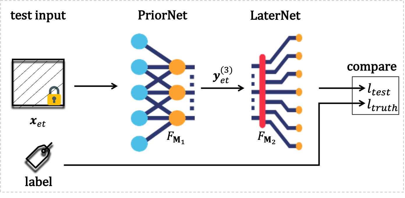
Figure 2: Pipeline of PriorNet and LaterNet inference.

We now elaborate in Fig. 2 the pipeline of PriorNet and LaterNet inference over a given test input encrypted under a tester’s public key of homomorphic encryption. We note that the corresponding label of the test input is not encrypted. Concretely, PriorNet is privately performed by the developer. It takes as input an encrypted test $\textbf{X}_{et}\in\mathcal{R}_{q}$, and produces an FHE-encrypted intermediate result $\textbf{Y}^{(3)}_{et}\in\mathcal{R}_{q}$ as the output. Since the homomorphic encryption cannot efficiently support the operations beyond additions and multiplications [39, 30], the activation layer within the PriorNet is approximated by a $2$-degree polynomial function.

Successively, $\textbf{Y}^{(3)}_{et}$’s plaintext $\textbf{Y}^{(3)}$ will be fed into the LaterNet $F_{\textbf{M}_{2}}$ whose computations are delegated to a service provider. We can leverage the re-encryption technique to let the service provider obtain the plaintext $\textbf{Y}^{(3)}$. Since the computations are conducted on plaintext domain, the later activation functions remain unchanged. Finally, LaterNet outputs the prediction result $l_{\textsf{test}}$. The service provider proceeds to compare the previously given true label $l_{\textsf{truth}}$ with $l_{\textsf{test}}$, and returns an equality indicator $0$ or $1$. For a batch of test data, he would count the number of $1$ indicator, and return a proportion of correct prediction. For the case of using a posterior probability vector as a prediction output, we determine the indicator value according to the distance between the prediction output and the corresponding truth.

IV-B Basic Workflow

We consider four main entities—public platform (PP), model tester (MT), model developer (MD) and service provider (SP) as demonstrated in Fig. 3.

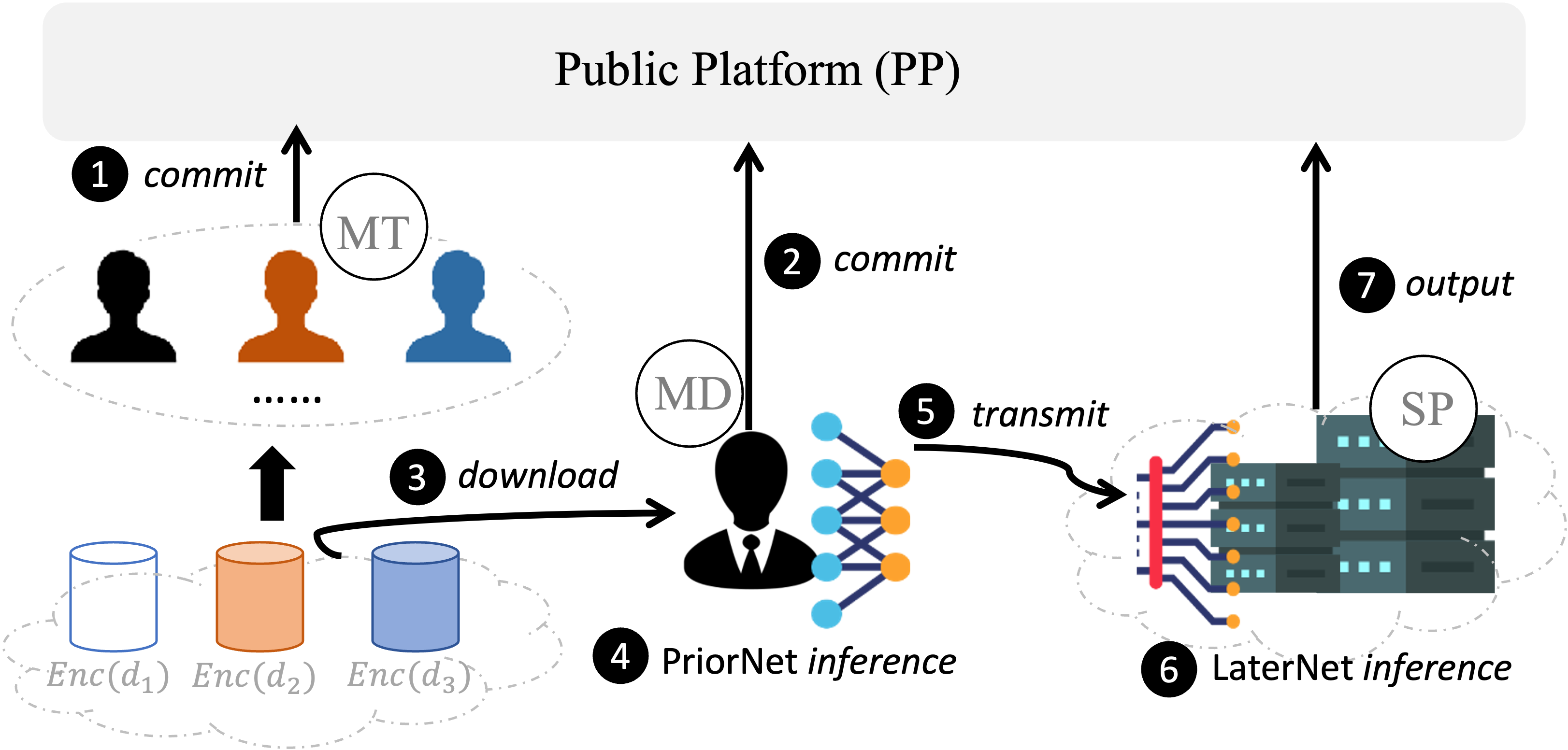
Figure 3: Scenario overview of pvCNN

Specifically, the PP in real world may refer to a publicly accessible and online platform, which can be maintained by a set of computational nodes. On the platform, an MD is allowed to advertise his/her pre-trained CNN model by announcing some usage descriptions and model performance, so as to attract users of interest for earning profits, while an MT can provide test data for measuring the model performance. In order to establish trust among the MD, the MT and future users in the scenario, the pvCNN wants to enable verifiable announcements on the public platform, that is, any future user is assured of the truthfulness of model performance without learning any information of either private model parameters or test data. We note the MD can delegate computation-consuming tasks to the powerful SP.

The basic workflow around the entities is shown below:  ➊ MTs freely participate in the platform and commit to the test data. They also store encrypted test data by using a leveled FHE (L-FHE) scheme [50] on the publicly accessible server.  ➋ The MD splits his CNN model into a private PriorNet which is kept at local device, as well as, a public LaterNet which is sent to the SP; After that, he generates two commitments to the PriorNet and LaterNet, and sends them to the PP.  ➌ The MD downloads the ciphered test data.  ➍ The MD evaluates the plaintext PriorNet on the encrypted test data and generates a proof of executing the inference computation as promised.  ➎ The MD sends the encrypted output of the Step ➍. Note that the encrypted output can be transformed into the ciphertext under the SP’s public key via re-encryption.  ➏ The SP successively runs LaterNet inference in the clear by taking the plaintext output of PriorNet inference as inputs, and proves that LaterNet is executed correctly with the true inputs and meanwhile LaterNet is consistent to the committed one.  ➐ The SP submits the final test results (e.g., classification correctness rate) to the platform, and distributes proofs to the decentralized nodes for proofs aggregation and validation.

IV-C Threat Assumptions

Model Developers. We consider CNN developers are untrusted; they can provide untruthful prediction results, e.g., outputting meaningless predictions or using arbitrary test data or CNN model. They can also be curious about test data during a CNN testing. Note that our verifiable computing design does not focus on poisoned or backdoored models[51], but it greatly relies on multi-tester test data to probe the performance of CNN models in a black-box manner. Recently, SecureDL[52] and VerIDeep[53] resort to sensitive samples to detect model changes, which can be complementary to our work.

Service Providers. They can be computationally powerful entities, and accept outsourced LaterNet from developers. Despite service providers’ powerful capabilities on computation and storage, we do not trust them. They can try their best to steal private information with regard to PriorNet and test inputs. They even incorrectly run LaterNet and produce untruthful results due to machine disruption. Service providers can also collude with a developer to fake correctness proofs, with respect to the independent inference processes based on a splitting CNN, aiming to evade verification by later-coming users. But the service providers cannot obtain PriorNet by colluding with the developer, since the developer has no motivation. Similar to previous studies [16, 15], we do not account for hyper-parameter extraction attacks through side-channel analysis [54, 55] from service providers in our research. Instead, we assume hyper-parameters to be publicly accessible in our setting. Moreover, there are defensive methods available [56] to mitigate such side-channel analysis attacks .

Model Testers. Testers are organized via a crowdsourcing manner. We consider that the testers are willing to contribute their test inputs for measuring the quality of the CNNs. A tester’s test inputs concretely contain a batch of data on an input-label basis. We assume the original inputs need protected but their labels can be public (refer to encrypted inputs and plaintext labels in Section IV-A). We also assume each label is consistent with the corresponding input’s true label, considering currently popular crowdsourcing-empowered label platforms.

Public Platform and Future Users. We assume both the public platform and future users are honest. Users have access to all of data (not including model parameters or test data) uploaded to the platform and the data cannot be tampered. Finally, we assume that all entities communicate via a secure authenticated channel.

V CONCRETE DESIGN

This section will introduce how to generate publicly verifiable zk-SNARK proofs for CNN testing based on L-FHE and collaborative inference. We will present high-level ideas in the subsection V-A. We then illustrate the optimization for 2-D convolutional relations in the subsection V-B. In the subsequent subsection V-C, we generate zk-SNARK proofs for a whole CNN testing process in a divide-and-conquer fashion, and aggregate multiple proofs in the subsection V-D.

V-A High-level Ideas

On top of the scenario of testing PriorNet and LaterNet with encrypted test data from testers, we want to generate zk-SNARK proofs for convincing any future user that (1) the model developer correctly runs PriorNet on the ciphered test data and returns the ciphered intermediate result as output; and (2) the service provider exactly takes the intermediate result as input and correctly accomplishes the successive computations of LaterNet, which produces a correct result. Meanwhile, any future user does not learn any information about the model parameters, the intermediate result and the test data.

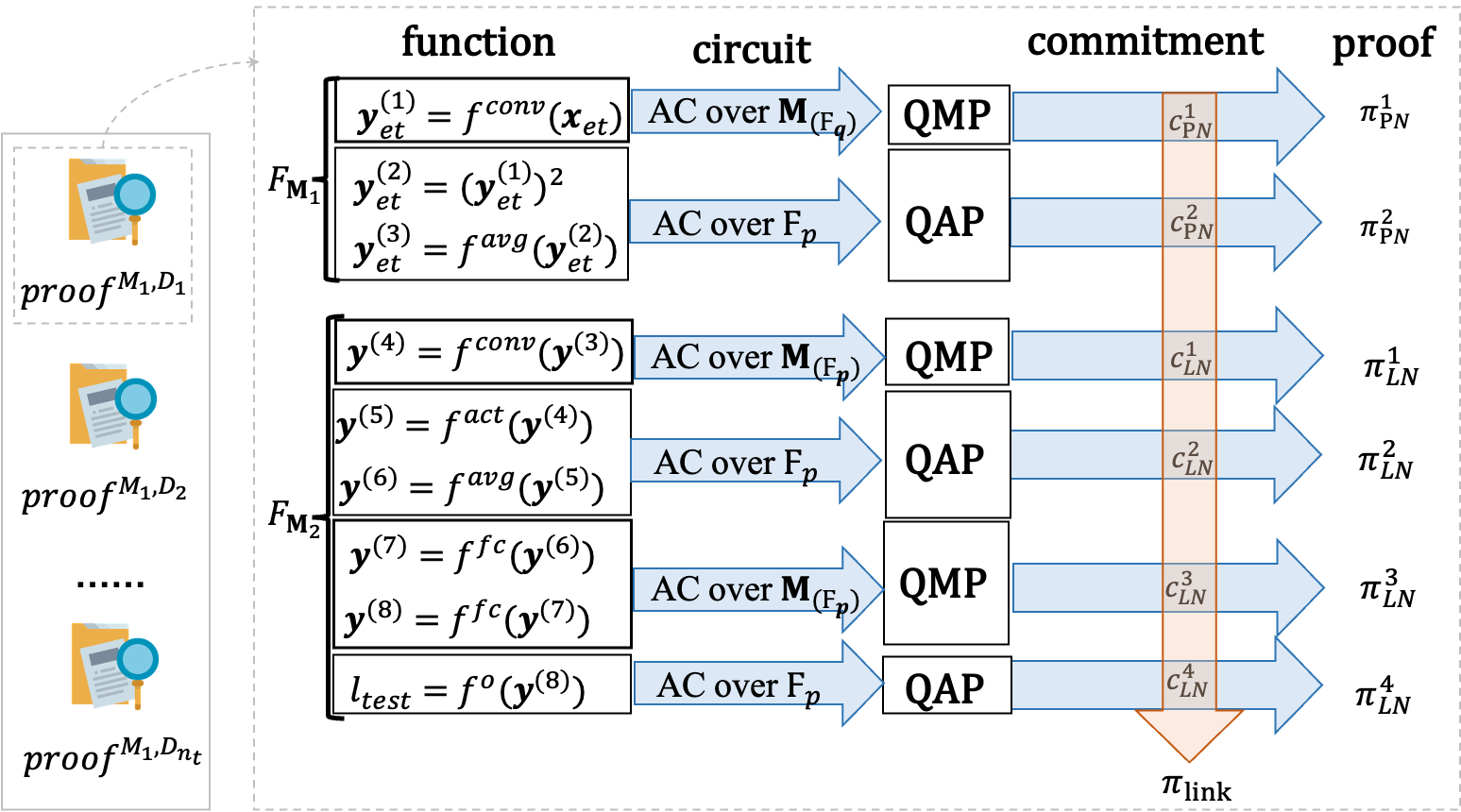
Figure 4: Overview of proof generation. See the column of function, we use a 2-degree polynomial to approximate the ReLU function in the PriorNet $F_{\textbf{M}_{1}}$.

Most importantly, we make two efforts to improve proving and verification costs, by reducing the number of multiplication gates and compressing multiple proofs, respectively. For ease of understanding, we firstly introduce a roadmap of proof generation, and then particularly emphasize our two efforts during proof generation. As shown in Fig. 4, the roadmap of generating QAP-based zkSNARK proofs is: a) compiling the functions of the splitting CNN testing into circuits, b) expressing the circuits as a set of QAPs, c) constructing the zk-SNARK proofs for the QAPs, and d) generating commitments for linking together the zk-SNARK proofs which are constructed separately. Based on the roadmap, our main efforts include: (A) Optimizing convolutional relations for b) (see Section V-B). We allow matrices in constructing the QAP, leading to quadratic matrix programs (QMP) [31], which is inspired by vCNN[12]’s efforts of applying polynomials into QAP (QPPs, quadratic polynomial programs [57]). Our QMP can optimize convolutional relations, considering a convolution layer with multiple filters and inputs can be strategically represented by a single matrix multiplication operation. The operation of matrix multiplication then is complied into the arithmetic circuits in QMP with only a single multiplication gate. As a consequence, the number of multiplication gates dominating proving costs is greatly reduced, compared to the previous case of using the original expression of QAP. (B) Aggregating proofs for c) (see Section V-D). We enable aggregating multiple proofs for different statements respective to test datasets over the same QAP/QMP for the same CNN model. The single proof after aggregation then is validated by a secure committee and the validity result based on the majority voting will be submitted and recorded on our public platform. In such way, any future user only needs to check the validation result to determine whether or not the statements over the CNN are valid.

V-B Optimizing Convolutional Relations

As demonstrated in Fig. 5, we consider 2-D convolution operations between $Mn^{2}$ amount of $n\times n$ input matrices and $M$ amount of $m\times m$ convolution filters (herein, $M>n$), which produces $M^{2}n^{2}$ filtered matrices of $(n-m+1)\times(n-m+1)$, by setting the stride $1$. Specifically, by computing the inner products between each input matrix and each filter matrix, $\forall i,j\in[0,n-m]$ and $k\in[0,M-1]$, it can be expressed as: $\textbf{Y}^{k}[i][j]=\sum_{l_{r}=0,l_{c}=0}^{m-1,m-1}\textbf{X}[i+l_{r}][j+l_{c}]\times\textbf{W}^{k}[l_{r}][l_{c}].$ Obviously, the multiplication complexity of such inner product computation is $O(n^{2}\cdot m^{2})$. Note that there are $M\cdot Mn^{2}$ amount of such set of Y, with respect to $Mn^{2}$ inputs and $M$ filters. Thus, $O(M\cdot Mn^{2}\cdot(n^{2}\cdot m^{2}))$ multiplication gates in QAP-based circuits are needed for handling $Mn^{2}$ inputs and $M$ filters. Since the proving time depends on the number of multiplication gates, a proof generation process for 2-D convolution operations becomes impractical.

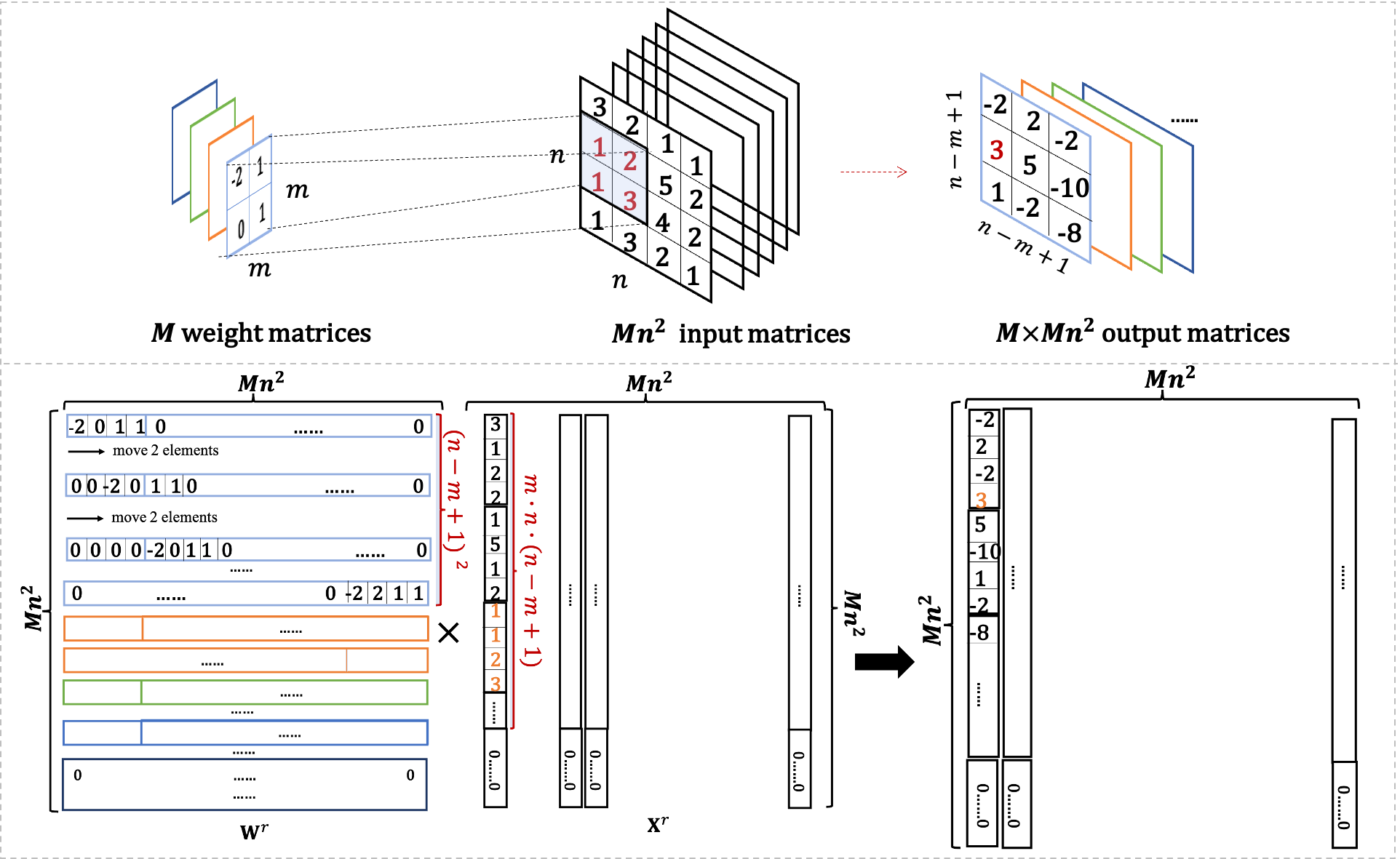
Figure 5: Matrix multiplication for convolution operations. We transform the convolution operations of $M$ weight matrices and $Mn^{2}$ input matrices (demonstrated on the top) into the matrix multiplication operation between two square matrices of $Mn^{2}\times Mn^{2}$ (demonstrated on the bottom).

Now, we seek for improving proving efficiency by reducing the multiplication complexity to $O(Mn^{2}\cdot Mn^{2})$. The very first step is to represent the inner products between the $Mn^{2}$ inputs and $M$ filters with a single matrix multiplication. Concretely, we show a concrete example of the representation in Fig. 5. First, given $Mn^{2}$ amount of $n\times n$ input matrices $\{\textbf{X}\}$, they are reshaped into a square matrix $\textbf{X}^{r}$ of $Mn^{2}\times Mn^{2}$. Second, another square matrix $\textbf{W}^{r}$ of the same dimension can be constructed by packing the $M$ filter matrices in a moving and zero padding manner. As a result, the multiplication between the two square matrices produces a square matrix $\textbf{Y}^{r}$ of $Mn^{2}\times Mn^{2}$, which can also be regarded as a reshaped matrix from the original $M\cdot Mn^{2}$ amount of output matrices. Based on such representation, the two square matrices $\textbf{W}^{r}$ and $\textbf{X}^{r}$ of the matrix multiplication can later be the left and right inputs of an arithmetic circuit with only one multiplication gate. We proceed to express the above circuit with our new QMP by using matrices in QAP, which follows the similar principle of using polynomials in QAP [57].

QMP Definition [31]. For an arithmetic circuit with $n_{in}$ input variables, $n_{ot}$ output variables in $\textbf{M}_{(\mathtt{F}_{p})}^{s\times s}$ and $n_{*}$ multiplication gates, a QMP is consisting of three sets of polynomials $\{L_{i}(x),R_{i}(x),O_{i}(x)\}_{i=0}^{m}$ with coefficients in $\textbf{M}_{(\mathtt{F}_{p})}^{s\times s}$ and a $n_{*}$-degree target polynomial $t(x)\in\mathtt{F}_{p}[x]$. $\mathtt{F}_{p}$ is a large finite field, e.g., $2^{254}$. The QMP computes the arithmetic circuit and $(\textbf{A}_{0},...,\textbf{A}_{n_{in}},\textbf{A}_{m-n_{ot}+1},...,\textbf{A}_{m})\in\textbf{M}_{(\mathtt{F}_{p})}^{s\times s}$ is valid assignment for the $n_{in}+n_{ot}$ input/output variables iff there exists $m-n_{in}-n_{ot}$ coefficients $(\textbf{A}_{n_{in}+1},...,\textbf{A}_{m-n_{ot}})\in\textbf{M}_{(\mathtt{F}_{p})}^{s\times s}$ for arbitrary $\textbf{X}\in\textbf{M}_{(\mathtt{F}_{p})}^{s\times s}$ such that $t(x)$ divides $p(x,\textbf{X})=\textsf{tr}\{\textbf{X}^{T}\sum_{i=0}^{m}\textbf{A}_{i}L_{i}(x))\cdot\sum_{i=0}^{m}\textbf{A}_{i}R_{i}(x)\}-\textsf{tr}\{\textbf{X}^{T}\sum_{i=0}^{m}\textbf{A}_{i}O_{i}(x)\}.$ Herein, tr means the trace of a square matrix, and the degree of the QMP is $deg(t(x))$. We note that each wire of the arithmetic circuit is labeled by a square matrix $\textbf{A}_{i}\in\textbf{M}_{(\mathtt{F}_{p})}^{s\times s}$. Suppose that the arithmetic circuit contains $n_{*}$ multiplication gates, and then $t(x)=\prod_{r=0}^{n_{*}-1}t(x-x_{r})$. With regard to a multiplication gate $x_{r}$, its left input wire is labeled by $\sum_{i=0}^{m}\textbf{A}_{i}L_{i}(x_{r}))$, right input wire is labeled by $\sum_{i=0}^{m}\textbf{A}_{i}R_{i}(x_{r}))$, and the output wire is $\sum_{i=0}^{m}\textbf{A}_{i}O_{i}(x_{r}))$. We note that the multiplication gate is constrained by $\textsf{tr}\{\textbf{X}^{T}\sum_{i=0}^{m}\textbf{A}_{i}L_{i}(x_{r}))\cdot\sum_{i=0}^{m}\textbf{A}_{i}R_{i}(x_{r})\}=\textsf{tr}\{\textbf{X}^{T}\sum_{i=0}^{m}\textbf{A}_{i}O_{i}(x_{r})\}.$

Part 1: Layer-wise prediction correctness for PriorNet. Step 1: to prove that the prover knows the openings of the commitments in $\textsf{st}_{\textsf{PN}}^{S1}$ $\mathtt{R}_{\textsf{PN}}^{S1}:=\big{\{}(\textsf{st}_{\textsf{PN}}^{S1}=(C_{\textsf{L}_{1}},C_{\textbf{X}},C_{\textsf{PN}}^{inter},\underline{C_{\textsf{L}_{1},k},C_{\textsf{L}_{2},k},C_{\textsf{L}_{3},k}},k,{\color[rgb]{0.68,0.09,0.13}ck^{\textsf{S1}},ck_{\textsf{PN}}}),\textsf{wt}_{\textsf{PN}}^{S1}=(\textbf{W}_{ed}^{r(1)},\textbf{X}_{et}^{r(1)},\textbf{Y}_{et}^{r(1)},\textbf{Y}_{et}^{r(2)},\textbf{Y}_{et}^{r(3)},\underline{\textbf{W}_{ed,k}^{r(1)},\textbf{X}_{et,k}^{r(1)},\textbf{Y}_{et,k}^{r(1)},\textbf{Y}_{et,k}^{r(2)},\textbf{Y}_{et,k}^{r(3)}},\mathbf{r}_{\textsf{PN}})\mid$ $\textbf{W}_{ed,k}^{r(1)}=\textbf{W}_{ed}^{r(1)}(k)\wedge\textbf{X}_{et,k}^{r(1)}=\textbf{X}_{et}^{r(1)}(k)\wedge\textbf{Y}_{et,k}^{r(1)}=\textbf{Y}_{et}^{r(1)}(k)\wedge\textbf{Y}_{et,k}^{r(2)}=\textbf{Y}_{et}^{r(2)}(k)\wedge\textbf{Y}_{et,k}^{r(3)}=\textbf{Y}_{et}^{r(3)}(k)$ $\wedge C_{\textsf{L}_{1}}=\textsf{MPoly.Com}(\textbf{W}_{ed}^{r(1)},{\color[rgb]{0.68,0.09,0.13}ck^{\textsf{S1}}},\mathbf{r}_{\textsf{PN}})\wedge C_{\textbf{X}}=\textsf{MPoly.Com}(\textbf{X}_{et}^{r(1)},{\color[rgb]{0.68,0.09,0.13}ck^{\textsf{S1}}},\mathbf{r}_{\textsf{PN}})\wedge C_{\textsf{PN}}^{inter}=\textsf{MPoly.Com}(\textbf{Y}_{et}^{r(1)},\textbf{Y}_{et}^{r(2)},\textbf{Y}_{et}^{r(3)},{\color[rgb]{0.68,0.09,0.13}ck_{\textsf{PN}}},\mathbf{r}_{\textsf{PN}})$ $\wedge\underline{C_{\textsf{L}_{1},k}=\textsf{MPoly.Com}(\textbf{W}_{ed,k}^{r(1)},\textbf{X}_{et,k}^{r(1)},\textbf{Y}_{et,k}^{r(1)},{\color[rgb]{0.68,0.09,0.13}ck_{\textsf{PN}}},\mathbf{r}_{\textsf{PN}})}$ $\wedge\underline{C_{\textsf{L}_{2},k}=\textsf{MPoly.Com}(\textbf{Y}_{et,k}^{r(2)},{\color[rgb]{0.68,0.09,0.13}ck_{\textsf{PN}}},\mathbf{r}_{\textsf{PN}})}\wedge\underline{C_{\textsf{L}_{3},k}=\textsf{MPoly.Com}(\textbf{Y}_{et,k}^{r(3)},{\color[rgb]{0.68,0.09,0.13}ck_{\textsf{PN}}},\mathbf{r}_{\textsf{PN}})}\big{\}}.$ //$ck_{\textsf{PN}}$ is the commitment key used before the evaluation while $ck^{\textsf{S1}}$ is used during the prediction //$C_{\textbf{X}}$ commits to $\textbf{X}_{et}^{r(1)}$; $C_{\textsf{L}_{1}}$ commits to $\textbf{W}_{ed}^{r(1)}$ Step 2: to prove that the equations with respect to $\textsf{L}_{1},\textsf{L}_{2},\textsf{L}_{3}$ hold $\mathtt{R}_{\textsf{PN}}^{S2}[\textsf{L}_{1}]:=\big{\{}(\textsf{st}_{\textsf{PN}}^{S2}=(C_{\textsf{L}_{1},k}^{{}^{\prime}},k,{\color[rgb]{0.68,0.09,0.13}ck_{\textsf{L}_{1}}}),\textsf{wt}_{\textsf{PN}}^{S2}=(\textbf{W}_{ed,k}^{r(1)},\textbf{X}_{et,k}^{r(1)},\textbf{Y}_{et,k}^{r(1)},\textbf{r}_{\textsf{PN}}))\mid\textbf{Y}_{et,k}^{r(1)}=\textbf{W}_{ed,k}^{r(1)}\odot\textbf{X}_{et,k}^{r(1)}\wedge~{}C_{\textsf{L}_{1},k}^{{}^{\prime}}=\textsf{MPoly.Com}(\textbf{W}_{ed,k}^{r(1)}),\textbf{X}_{et,k}^{r(1)},\textbf{Y}_{et,k}^{r(1)},{\color[rgb]{0.68,0.09,0.13}ck_{\textsf{L}_{1}}},\textbf{r}_{\textsf{PN}})\big{\}}.$ //$ck_{\textsf{L}_{1}}$ is built depending on the relation; $C_{\textsf{L}_{1},k}^{{}^{\prime}}$ commits to the consistent $\textbf{W}_{ed,k}^{r(1)}),\textbf{X}_{et,k}^{r(1)},\textbf{Y}_{et,k}^{r(1)}$ with the above $C_{\textsf{L}_{1},k}$ $\mathtt{R}_{\textsf{PN}}^{S2}[\textsf{L}_{2},\textsf{L}_{3}]:=\big{\{}(\textsf{st}_{\textsf{PN}}^{S2}=(C_{\textbf{L}_{2},k}^{{}^{\prime}},C_{\textbf{L}_{2}}[\textbf{Y}_{et,k}^{r(1)}],C_{\textbf{L}_{3},k}^{{}^{\prime}},C_{\textbf{L}_{3}}[\textbf{Y}_{et,k}^{r(2)}],k,{\color[rgb]{0.68,0.09,0.13}ck_{\textsf{L}_{2}}},{\color[rgb]{0.68,0.09,0.13}ck_{\textsf{L}_{3}}}),\textsf{wt}_{\textsf{PN}}^{S2}=(\textbf{Y}_{et,k}^{r(2)},\textbf{Y}_{et,k}^{r(3)},\mathbf{r}_{\textsf{PN}})\mid$ $\{\textbf{Y}^{r(2)}_{et,k}[i][j]=(\textbf{Y}^{r(1)}_{et,k}[i][j])^{2}+\textbf{Y}^{r(1)}_{et,k}[i][j]\}_{i=0,j=0}^{Mn^{2}-1,Mn^{2}-1}\wedge\textbf{Y}^{r(3)}_{et,k}=f^{\text{avg}}(\textbf{Y}^{r(2)}_{et,k})\wedge~{}C_{\textbf{L}_{2},k}^{{}^{\prime}}=\textsf{MPoly.Com}(\textbf{Y}_{et,k}^{r(2)},{\color[rgb]{0.68,0.09,0.13}ck_{\textsf{L}_{2}}},\mathbf{r}_{\textsf{PN}})$ $\wedge C_{\textbf{L}_{2}}[\textbf{Y}_{et,k}^{r(1)}]=\textsf{MPoly.Com}(\textbf{Y}_{et,k}^{r(1)},{\color[rgb]{0.68,0.09,0.13}ck_{\textsf{L}_{2}}},\mathbf{r}_{\textsf{PN}})\wedge C_{\textbf{L}_{3},k}^{{}^{\prime}}=\textsf{MPoly.Com}(\textbf{Y}_{et,k}^{r(3)},{\color[rgb]{0.68,0.09,0.13}ck_{\textsf{L}_{3}}},\mathbf{r}_{\textsf{PN}})\wedge C_{\textbf{L}_{3}}[\textbf{Y}_{et,k}^{r(2)}]=\textsf{MPoly.Com}(\textbf{Y}_{et,k}^{r(2)},{\color[rgb]{0.68,0.09,0.13}ck_{\textsf{L}3}},\mathbf{r}_{\textsf{PN}})\big{\}}.$ //$C_{\textbf{L}_{2},k}^{{}^{\prime}}$ (and $C_{\textbf{L}_{3},k}^{{}^{\prime}}$) commit to the same $\textbf{Y}_{et,k}^{r(2)}$ (resp. $\textbf{Y}_{et,k}^{r(3)}$) with $C_{\textbf{L}_{2},k}$ (resp. $C_{\textbf{L}_{3},k}$) //$C_{\textbf{L}_{2}}[\textbf{Y}_{et,k}^{r(1)}]$ should commit to the same $\textbf{Y}_{et,k}^{r(1)}$ that $C_{\textsf{L}_{1},k}^{{}^{\prime}}$ commits to; similarly, $C_{\textbf{L}_{3}}[\textbf{Y}_{et,k}^{r(2)}]$ should commit to the same $\textbf{Y}_{et,k}^{r(2)}$ that $C_{\textsf{L}_{2},k}^{{}^{\prime}}$ commits to

Figure 6: Layer-by-layer relation definition for PriorNet.

Part 2: Layer-wise prediction correctness for LaterNet. $\mathtt{R}_{\textsf{LN}}[\textsf{L}_{4}]:=\big{\{}(\textsf{st}_{\textsf{LN}}=(C_{\textbf{Y}^{r(3)}},C_{\textsf{L}_{4}},C_{\textbf{Y}^{r(4)}},{\color[rgb]{0.68,0.09,0.13}ck_{\textsf{L}_{4}}}),~{}\textsf{wt}_{\textsf{LN}}=(\textbf{W}^{r(4)},\textbf{Y}^{r(3)},\textbf{Y}^{r(4)},\mathbf{r}_{\textsf{LN}}))\mid\textbf{Y}^{r(4)}=\textbf{W}^{r(4)}\times\textbf{Y}^{r(3)}$ $\wedge~{}C_{\textbf{Y}^{r(3)}}=\textsf{MPoly.Com}(\textbf{Y}^{r(3)},{\color[rgb]{0.68,0.09,0.13}ck_{\textsf{L}_{4}}},\mathbf{r}_{\textsf{LN}})\wedge C_{\textsf{L}_{4}}=\textsf{MPoly.Com}(\textbf{W}^{r(4)},{\color[rgb]{0.68,0.09,0.13}ck_{\textsf{L}_{4}}},\mathbf{r}_{\textsf{LN}})\wedge C_{\textbf{Y}^{r(4)}}=\textsf{MPoly.Com}(\textbf{Y}^{r(4)},{\color[rgb]{0.68,0.09,0.13}ck_{\textsf{L}_{4}}},\mathbf{r}_{\textsf{LN}})\big{\}}.$ //$C_{\textbf{Y}^{r(3)}}$ should commit to $\textbf{Y}^{r(3)}$ whose encryption is committed in $C_{\textsf{PN}}^{inter}$ $\mathtt{R}_{\textsf{LN}}[\textsf{L}_{5},\textsf{L}_{6}]:=\big{\{}(\textsf{st}_{\textsf{LN}}=(C_{\textsf{L}_{5}}[\textbf{Y}^{r(4)}],C_{\textbf{Y}^{r(5)}},C_{\textsf{L}_{6}}[\textbf{Y}^{r(5)}],C_{\textbf{Y}^{r(6)}},{\color[rgb]{0.68,0.09,0.13}ck_{\textsf{L}_{5}}},{\color[rgb]{0.68,0.09,0.13}ck_{\textsf{L}_{6}}}),~{}\textsf{wt}_{\textsf{LN}}=(\textbf{Y}^{r(4)},\textbf{Y}^{r(5)},\textbf{Y}^{r(6)},\mathbf{r}_{\textsf{LN}}))\mid$ $\{\textbf{Y}^{r(5)}[i][j]=max(\textbf{Y}^{r(4)}[i][j],0)\}_{i=0,j=0}^{Mn^{2}-1,Mn^{2}-1}\wedge\textbf{Y}^{r(6)}=f^{\text{avg}}(\textbf{Y}^{r(5)})$ $\wedge~{}C_{\textsf{L}_{5}}[\textbf{Y}^{r(4)}]=\textsf{MPoly.Com}(\textbf{Y}^{r(4)},{\color[rgb]{0.68,0.09,0.13}ck_{\textsf{L}_{5}}},\mathbf{r}_{\textsf{LN}})\wedge C_{\textbf{Y}^{r(5)}}=\textsf{MPoly.Com}(\textbf{Y}^{r(5)},{\color[rgb]{0.68,0.09,0.13}ck_{\textsf{L}_{6}}},\mathbf{r}_{\textsf{LN}})$//$C_{\textsf{L}_{5}}[\textbf{Y}^{r(4)}]$ should commit to $\textbf{Y}^{r(4)}$ that is committed in $C_{\textbf{Y}^{r(4)}}$ of $\textsf{L}_{4}$ $\wedge C_{\textsf{L}_{6}}[\textbf{Y}^{r(5)}]=\textsf{MPoly.Com}(\textbf{Y}^{r(5)},{\color[rgb]{0.68,0.09,0.13}ck_{\textsf{L}_{6}}},\mathbf{r}_{\textsf{LN}})\wedge C_{\textbf{Y}^{r(6)}}=\textsf{MPoly.Com}(\textbf{Y}^{r(6)},{\color[rgb]{0.68,0.09,0.13}ck_{\textsf{L}_{6}}},\mathbf{r}_{\textsf{LN}})\big{\}}.$//$C_{\textsf{L}_{6}}[\textbf{Y}^{r(5)}]$ should commit to $\textbf{Y}^{r(5)}$ that is committed in $C_{\textbf{Y}^{r(5)}}$ of $\textsf{L}_{5}$ $\mathtt{R}_{\textsf{LN}}[\textsf{L}_{7},\textsf{L}_{8}]:=\big{\{}(\textsf{st}_{\textsf{LN}}=(C_{\textsf{L}_{7,8}},C_{\textsf{L}_{7}}[\textbf{Y}^{r(6)}],C_{\textsf{L}_{8}}[\textbf{Y}^{r(8)}],{\color[rgb]{0.68,0.09,0.13}ck_{\textsf{L}_{7,8}}}),~{}\textsf{wt}_{\textsf{LN}}=(\textbf{W}^{r(7)},\textbf{W}^{r(8)},\textbf{Y}^{r(6)},\textbf{Y}^{r(7)},\textbf{Y}^{r(8)},\mathbf{r}_{\textsf{LN}}))\mid$ $\textbf{Y}^{r(7)}=\textbf{Y}^{r(6)}\times\textbf{W}^{r(7)}$ $\wedge C_{\textsf{L}_{7,8}}=\textsf{MPoly.Com}(\textbf{W}^{r(7)},\textbf{W}^{r(8)},{\color[rgb]{0.68,0.09,0.13}ck_{\textsf{L}_{7,8}}},\mathbf{r}_{\textsf{LN}})\wedge C_{\textsf{L}_{7}}[\textbf{Y}^{r(6)}]=\textsf{MPoly.Com}(\textbf{Y}^{r(6)},{\color[rgb]{0.68,0.09,0.13}ck_{\textsf{L}_{7,8}}},\mathbf{r}_{\textsf{LN}})\wedge C_{\textsf{L}_{8}}[\textbf{Y}^{r(8)}]=\textsf{MPoly.Com}(\textbf{Y}^{r(8)},{\color[rgb]{0.68,0.09,0.13}ck_{\textsf{L}_{7,8}}},\mathbf{r}_{\textsf{LN}})\big{\}}.$ //$C_{\textsf{L}_{7}}[\textbf{Y}^{r(6)}]$ should commit to $\textbf{Y}^{r(6)}$ that is committed in $C_{\textbf{Y}^{r(6)}}$ of $\textsf{L}_{6}$ $\mathtt{R}_{\textsf{LN}}[\textsf{L}_{o}]:=\big{\{}(\textsf{st}_{\textsf{LN}}=(C_{\textsf{L}_{o}}[\textbf{Y}^{r(8)}],\textbf{l}_{test},{\color[rgb]{0.68,0.09,0.13}ck_{\textsf{L}_{o}}}),\textsf{wt}_{\textsf{LN}}=(\textbf{Y}^{r(8)}))\mid\textbf{l}_{test}[j]=\textsf{argmax}(\textbf{Y}^{r(8)}[j])\wedge~{}C_{\textsf{L}_{o}}[\textbf{Y}^{r(8)}]=\textsf{MPoly.Com}(\textbf{Y}^{r(8)},{\color[rgb]{0.68,0.09,0.13}ck_{\textsf{L}_{o}}},\mathbf{r}_{\textsf{LN}})\big{\}}.$ //$C_{\textsf{L}_{o}}[\textbf{Y}^{r(8)}]$ should commit to $\textbf{Y}^{r(8)}$ that is committed in $C_{\textbf{Y}^{r(8)}}$ of $\textsf{L}_{8}$

Figure 7: Layer-by-layer relation definition for LaterNet.

QMP for Matrix Multiplication Relations. As we introduced before, we can represent convolutional operations as matrix multiplication $\textbf{Y}^{r}=\textbf{W}^{r}\times\textbf{X}^{r}$, where $\textbf{Y}^{r},\textbf{X}^{r}$ and $\textbf{W}^{r}\in\textbf{M}_{(\mathtt{Z}_{p})}^{Mn^{2}\times Mn^{2}}$. It is noteworthy that we can use advanced quantization techniques to transform floating-point numbersm of 8-bit precision into unsigned integer numbers in [$0,255$], which adapts to a large finite field. Now according to the QMP definition, when the matrix multiplication computation is expressed by the arithmetic circuit over matrices, the corresponding QMP is $\{L_{\textbf{W}}(x),R_{\textbf{X}}(x),O_{\textbf{Y}}(x),t(x)\}$ of the arithmetic circuit. Herein, there are three input/output variables, and the degree of the QMP is one.

Similarly, we can apply our above idea into full connection operations, and finally the operations can also be expressed with similarly low-degree QMP.

V-C Proof Generation for a Whole CNN Testing

This section elaborates how to generate proofs based on the CaP zk-SNARK for ensuring the result correctness of executing PriorNet and LaterNet. The proofs convince an arbitrary user that PriorNet is correctly evaluated on the ciphered test inputs, and subsequently, LaterNet is correctly performed by taking the clear outputs of PriorNet as inputs, yielding correct results. We note that the processes of proof generation for the PriorNet and LaterNet are slightly different. For PriorNet, the values, such as weights, test inputs and outputs, are represented as polynomial ring elements, and we follow Fiore et al.’s work [22] to generate proofs for the computation over polynomial rings. For LaterNet, we generate zk-SNARK proofs for the computation over scalars. We will begin with relation definition, and then present concrete realization for generating proofs. In light of the nature of layer-by-layer computation of model inference, we will use a divide-and-conquer method to generate zk-SNARK proofs for each separate layer, and combine them as a whole via a commit-and-prove methodology.

Let us define some notations at the beginning. We let MPoly.Com be a polynomial commitment scheme from [22]. We denote $ck_{\textsf{PN}}$ and $ck_{\textsf{LN}}$ are the commitment keys used for committing to the PriorNet and LaterNet; $\mathbf{r}_{\textsf{PN}}$, $\mathbf{r}_{\textsf{LN}}$ are non-reused commitment randomnesses. $C_{\textbf{M}_{1,{ed}}}$ means the commitments to the inputs, weights, intermediates of $\textbf{M}_{1}$ while $C_{\textbf{M}_{2}}$ represents the commitments to the weights and intermediates of $\textbf{M}_{2}$.

Relation Definition. We define the relations $\mathtt{R}_{\textsf{PN}}$ and $\mathtt{R}_{\textsf{LN}}$ with regard to PriorNet and LaterNet execution correctness:

$$\mathtt{R}_{\textsf{PN}}:=\big{\{}(\textsf{st}_{\textsf{PN}} =(C_{\textbf{M}_{1,{ed}}},C_{\textbf{X}_{et}^{r(1)}},\textbf{Y}^{r(3)}_{et},ck_{\textsf{PN}}),$$

$$\textsf{wt}_{\textsf{PN}} =(\textbf{M}_{1,{ed}},\textbf{X}_{et},\mathbf{r}_{\textsf{PN}}))\mid\textbf{Y}^{r(1)}_{et}=\textbf{W}^{r(1)}_{ed}\odot\textbf{X}^{r(1)}_{et}$$

$$\wedge\{\textbf{Y}^{r(2)}_{et}[i][j] =(\textbf{Y}^{r(1)}_{et}[i][j])^{2}+\textbf{Y}^{r(1)}_{et}[i][j]\}_{i=0,j=0}^{Mn^{2}-1,Mn^{2}-1}$$

$$\wedge\textbf{Y}^{r(3)}_{et} =f^{\text{avg}}(\textbf{Y}^{r(2)}_{et})$$

$$\wedge C_{\textbf{M}_{1,{ed}}} =\textsf{MPoly.Com}(\textbf{M}_{1,{ed}},ck_{\textsf{PN}},\mathbf{r}_{\textsf{PN}})$$

$$\wedge C_{\textbf{X}_{et}} =\textsf{MPoly.Com}(\textbf{X}_{et}^{r(1)},ck_{\textsf{PN}},\mathbf{r}_{\textsf{PN}})\big{\}},$$

$$\mathtt{R}_{\textsf{LN}}:=\{(\textsf{st}_{\textsf{LN}} =(C_{\textbf{Y}^{r(3)}},C_{\textbf{M}_{2}},l_{test},ck_{\textsf{LN}}),$$

$$\textsf{wt}_{\textsf{LN}} =(\textbf{Y}^{r(3)},\textbf{M}_{2},\mathbf{r}_{\textsf{LN}}))\mid\textbf{Y}^{r(4)}=\textbf{W}^{r(4)}\times\textbf{Y}^{r(3)}$$

$$\wedge\{\textbf{Y}^{r(5)}[i][j] =max(\textbf{Y}^{r(4)}[i][j],0)\}_{i=0,j=0}^{Mn^{2}-1,Mn^{2}-1}$$

$$\wedge\textbf{Y}^{r(6)} =f^{\text{avg}}(\textbf{Y}^{r(5)})$$

$$\wedge\textbf{Y}^{r(7)} =\textbf{Y}^{r(6)}\times\textbf{W}^{r(7)}$$

$$\wedge\textbf{Y}^{r(8)} =\textbf{Y}^{r(7)}\times\textbf{W}^{r(8)}$$

$$\wedge~{}\textbf{l}_{test}[j] =\textsf{argmax}(\textbf{Y}^{r(8)}[j])$$

$$\wedge~{}C_{\textbf{Y}^{r(3)}} =\textsf{MPoly.Com}(\textbf{Y}^{r(3)},ck_{\textsf{LN}},\mathbf{r}_{\textsf{LN}})$$

$$\wedge~{}C_{\textbf{M}_{2}} =\textsf{MPoly.Com}(\textbf{M}_{2},ck_{\textsf{LN}},\mathbf{r}_{\textsf{LN}})\big{\}}.$$

Besides the relations, we further define layer-by-layer relations for proving the layer-wise computations of the $\mathtt{R}_{\textsf{PN}}$ and $\mathtt{R}_{\textsf{LN}}$ in Fig. 6 and 7. In Part 1, the layer-wise computations of the PriorNet performs in an encryption manner, so we define the relations to be proven with Setp 1 and Setp 2, as guided by the work [22]. In Part 2, the LaterrNet runs in a plaintext setting, so we define the corresponding relations similar to the above Setp 2 (not needing Setp 1). Lastly, in order to combine the layer-wise computations as a whole, we also denote the relations for ensuring that starting from the second layer, each layer’s inputs are consistent with the former layer’s outputs.

With the relations, we proceed to generate zk-SNARK proofs accordingly. At a high level, the computations of the PriorNet and LaterNet are proved correct iff both of binary relations $\mathtt{R}_{\textsf{PN}}$ and $\mathtt{R}_{\textsf{LN}}$ return $1$, which means $\mathtt{R}_{\textsf{PN}}$ and $\mathtt{R}_{\textsf{LN}}$ hold on the corresponding pairs of statement and witness $(\textsf{st},\textsf{wt})$. For $\mathtt{R}_{\textsf{PN}}$, we generate publicly verifiable proofs that $\textbf{Y}^{r(3)}_{et}$ is computed correctly in an encryption manner, with the trained parameters of PriorNet $\textbf{M}_{1,{ed}}$ and ciphered test inputs $\textbf{X}_{et}^{r(1)}$ through the sequential computations mentioned in the $\mathtt{R}_{\textsf{PN}}$. In the relation, the witnesses $\textbf{M}_{1,{ed}}$ and $\textbf{X}_{et}^{r(1)}$ are committed using the key $ck_{\textsf{PN}}$, and the generated commitments plus $\textbf{Y}^{r(3)}_{et}$ are treated as the public statement. For $\mathtt{R}_{\textsf{LN}}$, we generate proofs that LaterNet takes the correct plaintext $\textbf{Y}^{r(3)}$ and returns the correct inference result $l_{test}$ by conducting the sequential operations included in the $\mathtt{R}_{\textsf{LN}}$. Similarly, the witnesses $\textbf{M}_{2}$ and $\textbf{Y}^{r(3)}$ are committed using the key $ck_{\textsf{LN}}$, and then the commitments and the execution result are public statements. The processes of proof generation for $\mathtt{R}_{\textsf{PN}}$ and $\mathtt{R}_{\textsf{LN}}$ are conducted separately, since the two parts PriorNet and LaterrNet are executed by different entities. After completing the proofs for the two parts, we link the proofs together by additionally proving that the output of the PriorNet is exactly equal to the input of the LaterNet.

Step 1 CaP zk-SNARK Proofs of Knowledge of Commitments 1:  MUniEv-$\Pi$.Setup($\lambda,d_{c},n_{c})\rightarrow{\color[rgb]{0.68,0.09,0.13}ck^{S1}}:$ 2:  //$d_{c}$ refers to the degree of ciphers; $n_{c}$ is the number of ciphers 3:   $g,h\overset{\$}{\leftarrow}\mathtt{G}$, $g^{*}\overset{\$}{\leftarrow}\mathcal{G}$, $\alpha,s,t\overset{\$}{\leftarrow}\mathtt{Z}_{p}$ 4:   $\hat{g}=g^{\alpha},\hat{h}=h^{\alpha},\hat{g^{*}}={g^{*}}^{\alpha}$, $g^{*}_{1}={g^{*}}^{s}$, $h_{1}=h^{s}$, 5:   $\{g_{i,j}=g^{s^{i}t^{j}},\hat{g}_{i,j}=\hat{g}^{s^{i}t^{j}}\}_{i=0,j=0}^{d_{c},n_{c}}$, HASH: ${\mathtt{G}}^{*}\times{\mathtt{Z}_{q}}^{*}\rightarrow\mathtt{Z}_{p}$ 6:   ${\color[rgb]{0.68,0.09,0.13}ck^{S1}}:=(g,h,g^{*},\{g_{i,j},\hat{g}_{i,j}\}_{i=0,j=0}^{d_{c},n_{c}},\hat{g},\hat{h},\hat{g^{*}},g^{*}_{1},h_{1},\textsf{HASH})$ 7:  MUniEv-$\Pi$.Prove(${\color[rgb]{0.68,0.09,0.13}ck^{S1}},\textbf{W}^{r(1)}_{ed},\textbf{X}^{r(1)}_{et})\rightarrow\pi^{S1}:$ 8:  //$\textbf{W}^{r(1)}_{ed},\textbf{X}^{r(1)}_{et}$ are square matrices of $l_{\text{new}}=Mn^{2}$ 9:  //$l_{\text{new}}^{2}$ is smaller that $n_{c}$ 10:  //call the commitment scheme MPoly.Com of [22] 11:  $\textsf{call~{}MPoly.Com}({\color[rgb]{0.68,0.09,0.13}ck^{S1}},\textbf{W}^{r(1)}_{ed})\rightarrow C_{\textsf{W}_{1}}$: $-~{}r_{\textsf{W}_{1}}\overset{\$}{\leftarrow}\mathtt{Z}_{p}$, $-~{}C_{\textsf{W}_{1}}^{1}=h^{r_{\textsf{W}_{1}}}g_{i,j}^{\sum_{i=0,j=0}^{d_{c},l_{\text{new}}^{2}-1}w_{i,j}}$, $C_{\textsf{W}_{1}}^{2}=\hat{h}^{r_{\textsf{W}_{1}}}\hat{g}_{i,j}^{\sum_{i=0,j=0}^{d_{c},l_{\text{new}}^{2}-1}w_{i,j}}$, $-~{}C_{\textsf{W}_{1}}:=(C_{\textsf{W}_{1}}^{1},C_{\textsf{W}_{1}}^{2})$ 12:  $\textsf{call~{}MPoly.Com}({\color[rgb]{0.68,0.09,0.13}ck^{S1}},\textbf{X}^{r(1)}_{et})\rightarrow C_{\textbf{X}}$: $-~{}r_{\textbf{X}}\overset{\$}{\leftarrow}\mathtt{Z}_{p}$, $C_{\textbf{X}}^{1}=h^{r_{\textbf{X}}}g_{i,j}^{\sum_{i=0,j=0}^{d_{c},l_{\text{new}}^{2}-1}\text{x}_{i,j}}$, $C_{\textbf{X}}^{2}=\hat{h}^{r_{\textbf{X}}}\hat{g}_{i,j}^{\sum_{i=0,j=0}^{d_{c},l_{\text{new}}^{2}-1}\text{x}_{i,j}}$, $-~{}C_{\textbf{X}}:=(C_{\textbf{X}}^{1},C_{\textbf{X}}^{2})$ 13: $\textsf{call~{}MPoly.Com}({\color[rgb]{0.68,0.09,0.13}ck^{S1}},\textbf{Y}^{r(1)}_{et})\rightarrow C_{\textbf{Y}}$: $-~{}r_{\textbf{Y}}\overset{\$}{\leftarrow}\mathtt{Z}_{p}$, $C_{\textbf{Y}}^{1}=h^{r_{\textbf{Y}}}g_{i,j}^{\sum_{i=0,j=0}^{d_{c},l_{\text{new}}^{2}-1}\text{y}_{i,j}}$, $C_{\textbf{Y}}^{2}=\hat{h}^{r_{\textbf{Y}}}\hat{g}_{i,j}^{\sum_{i=0,j=0}^{d_{c},l_{\text{new}}^{2}-1}\text{y}_{i,j}}$, $-~{}C_{\textbf{Y}}:=(C_{\textbf{Y}}^{1},C_{\textbf{Y}}^{2})$ 14: $k=\textsf{HASH}(C_{\textsf{W}_{1}},C_{\textbf{X}},\textbf{W}^{r(1)}_{ed},\textbf{X}^{r(1)}_{et},\textbf{Y}^{r(1)}_{et})$ 15:  //$\textbf{X}^{r(1)}_{et}\in\textbf{M}_{\mathtt{Z}_{q}[x](x^{d_{c}}+1)}^{l_{new}^{2}}$, $\textbf{X}(x,y)=\sum_{i=0,j=0}^{d_{c},l_{\text{new}}^{2}-1}\text{x}_{i,j}x^{i}y^{j}$ 16:  //$\textbf{W}^{r(1)}_{et}\in\textbf{M}_{\mathtt{Z}_{q}[x](x^{d_{c}}+1)}^{l_{new}^{2}}$, $\textbf{W}(x,y)=\sum_{i=0,j=0}^{d_{c},l_{\text{new}}^{2}-1}\text{w}_{i,j}x^{i}y^{j}$ 17:  //$\textbf{Y}^{r(1)}_{et}\in\textbf{M}_{\mathtt{Z}_{q}[x](x^{d_{c}}+1)}^{l_{new}^{2}}$, $\textbf{Y}(x,y)=\sum_{i=0,j=0}^{d_{c},l_{\text{new}}^{2}-1}\text{y}_{i,j}x^{i}y^{j}$ 18: $\textsf{L}_{1}:=\textsf{L}_{1}(x,y)=\textbf{W}(x,y)+\textbf{X}(x,y)+\textbf{Y}(x,y)=\sum_{i=0,j=0}^{d_{c},l_{\text{new}}^{2}-1}l_{i,j}x^{i}y^{j}$ 19: $\textsf{call~{}MPoly.Com}({\color[rgb]{0.68,0.09,0.13}ck^{S1}},\textsf{L}_{1}(s,t))\rightarrow C_{\textsf{L}_{1}}=(C_{\textsf{L}_{1}}^{1},C_{\textsf{L}_{1}}^{2})$ 20: $\textsf{L}_{1,k}:=\textsf{L}_{1}(k,y)=\textbf{W}(k,y)+\textbf{X}(k,y)+\textbf{Y}(k,y)=\sum_{i=0,j=0}^{d_{c},l_{\text{new}}^{2}-1}l_{i,j}k^{i}y^{j}$ 21: $\textsf{call~{}MPoly.Com}({\color[rgb]{0.68,0.09,0.13}ck^{S1}},\textbf{W}^{r(1)}_{ed,k})\rightarrow C_{\textsf{w},k}=(C_{\textsf{w},k}^{1},C_{\textsf{w},k}^{2})$ 22: $\textsf{call~{}MPoly.Com}({\color[rgb]{0.68,0.09,0.13}ck^{S1}},\textbf{X}^{r(1)}_{ed,k})\rightarrow C_{\textsf{x},k}=(C_{\textsf{x},k}^{1},C_{\textsf{x},k}^{2})$ 23: $\textsf{call~{}MPoly.Com}({\color[rgb]{0.68,0.09,0.13}ck^{S1}},\textbf{Y}^{r(1)}_{ed,k})\rightarrow C_{\textsf{y},k}=(C_{\textsf{y},k}^{1},C_{\textsf{y},k}^{2})$ 24: $C_{\textsf{L}_{1},k}^{1}=(C_{\textsf{w},k}^{1}\cdot C_{\textsf{x},k}^{1}\cdot C_{\textsf{y},k}^{1});C_{\textsf{L}_{1},k}^{2}=(C_{\textsf{w},k}^{2}\cdot C_{\textsf{x},k}^{2}\cdot C_{\textsf{y},k}^{2})$ 25: $\textbf{T}(x,y)=\frac{\textsf{L}_{1}(x,y)-\textsf{L}_{1}(k,y)}{(x-k)}$ 26: $\bar{g}=\frac{h_{1}}{h^{k}}$, $a,b\overset{\$}{\leftarrow}\mathtt{Z}_{p}$, 27: $\textsf{call~{}MPoly.Com}({\color[rgb]{0.68,0.09,0.13}ck^{S1}},\textbf{T}(x,y))\rightarrow C_{\textbf{T}}$: $-~{}r_{\textbf{T}}\overset{\$}{\leftarrow}\mathtt{Z}_{p}$, $C_{\textbf{T}}^{1}=h^{r_{\textbf{T}}}\bar{g}^{\sum_{t=0,i=0,j=0}^{d_{c}-1,d_{c}-t,l_{\text{new}}^{2}-1}l_{i+t,j}k^{i-1}s^{i}t^{j}}$, $C_{\textbf{T}}^{1}=h^{r_{\textbf{T}}}\hat{\bar{g}}^{\sum_{t=0,i=0,j=0}^{d_{c}-1,d_{c}-t,l_{\text{new}}^{2}-1}l_{i+t,j}k^{i-1}s^{i}t^{j}}$, $-~{}C_{\textbf{T}}:=(C_{\textbf{T}}^{1},C_{\textbf{T}}^{2})$ 28: $U=e(h^{a}\bar{g}^{b},g^{*})$, $\mathtt{e}\leftarrow\textsf{HASH}(C_{\textsf{L}_{1}},C_{\textsf{L}_{1},k},C_{\textbf{T}},U,k)$, 29: $\sigma=a-(r_{\textbf{L}_{1},k}-r_{\textbf{L}_{1}})\cdot\mathtt{e}~{}\text{mod}~{}q$, $\tau=b-r_{\textbf{T}}\cdot\mathtt{e}~{}\text{mod}~{}q$, $\pi^{S1}=(C_{\textbf{T}},\mathtt{e},\sigma,\tau)$ 30: MUniEv-$\Pi$.Verify(${\color[rgb]{0.68,0.09,0.13}ck^{S1}},C_{\textsf{L}_{1}},C_{\textbf{X}},C_{\textsf{L}_{1},k},C_{\textbf{T}},k,\pi^{\textsf{S1}})\rightarrow 0/1$: 31: $b_{1}:=(e(C_{\textsf{L}_{1}}^{1},\hat{g^{*}})==e(C_{\textsf{L}_{1}}^{2},g^{*}))$; $b_{2}:=(e(C_{\textbf{X}}^{1},\hat{g^{*}})==e(C_{\textbf{X}}^{2},g^{*}))$; 32: $b_{3}:=(e(C_{\textbf{w},k}^{1},\hat{g^{*}})==e(C_{\textbf{w},k}^{2},g^{*})\wedge e(C_{\textbf{x},k}^{1},\hat{g^{*}})==e(C_{\textbf{x},k}^{2},g^{*})$ $\wedge e(C_{\textbf{y},k}^{1},\hat{g^{*}})==e(C_{\textbf{y},k}^{2},g^{*}))$; 33: $b_{4}:=(e(C_{\textbf{T}}^{1},\hat{g^{*}})==e(C_{\textbf{T}}^{2},g^{*}))$; 34: $H=e(C_{\textbf{T}}^{1},g^{*}_{1}/{g^{*}}^{k})\cdot e(C_{\textbf{L}_{1}}^{1}/C_{\textbf{L}_{1},k}^{1},g^{*})^{-1}$, $\bar{g}=h_{1}/h^{k}$, 35: $U=e(h^{\sigma}\bar{g}^{\tau},g^{*})\cdot H^{\mathtt{e}}$, 36: $b_{5}:=(\mathtt{e}==\textsf{HASH}(C_{\textbf{L}_{1}},C_{\textbf{L}_{1},k},C_{\textbf{T}},U,k))$; 37: $b=(b_{1}\wedge b_{2}\wedge b_{3}\wedge b_{4}\wedge b_{5})\rightarrow 0/1$.

Figure 8: Generating zk-SNARK proofs for relation $\mathtt{R}_{\textsf{PN}}^{S1}$.

Step 2 CaP zk-SNARK Proofs over QMP //st=($\textbf{W}^{r(1)}_{ed,k}$, $\textbf{X}^{r(1)}_{et,k}$, $\textbf{Y}^{r(1)}_{et,k}$);   $io=m=3$; QMP=($L(x)$,$R(x)$,$O(x)$,$t(x)$) //$p(x,\textbf{Z})=\textsf{tr}\{\textbf{Z}^{T}\cdot L(x)\cdot R(x)\}-\textsf{tr}\{\textbf{Z}^{T}\cdot O(x)\}=h(x,\textbf{Z})t(x)$, $\forall~{}\textbf{Z}\in\textbf{M}_{(\mathtt{Z}_{p})}^{l_{new}^{2}}$ 1: AC-$\Pi$.Setup($1^{\lambda}$, QMP)$\rightarrow\textsf{crs}$: 2: $(\alpha,\beta,\gamma,\delta,\eta,z)\leftarrow\mathtt{Z}_{p}$, $\textbf{Z}\leftarrow\textbf{M}_{(\mathtt{Z}_{p})}^{l_{new}^{2}}$, $g,h\leftarrow\mathtt{G}$ 3: $\textsf{crs}:=(g,h,g^{\alpha},g^{\beta},h^{\beta},h^{\gamma},g^{\delta},h^{\delta},g^{\frac{\eta}{\delta}},g^{\frac{\eta}{\gamma}},\{\textsf{OP}_{i}=g^{\frac{\beta L_{i}(z)}{\gamma}}\cdot g^{\frac{\alpha R_{i}(z)}{\gamma}}\cdot g^{\frac{O_{i}(z)}{\gamma}}\}_{i=0}^{t})$ 4: AC-$\Pi$.Prove(crs, st,wt)$\rightarrow\pi^{S2}_{\textsf{L}_{1}}$: 5: $L(x)=\cdot\textbf{W}^{r(1)}_{ed,k}\cdot L_{\textbf{W}}(z)$; $R(x)=\textbf{X}^{r(1)}_{et,k}\cdot R_{\textbf{X}}(z)$; $O(x)=\cdot\textbf{Y}^{r(1)}_{et,k}\cdot O_{\textbf{Y}}(z)$ 6: $(t,s,v)\overset{\$}{\leftarrow}\mathtt{Z}_{p}$, $A:=g^{\alpha}\cdot g^{\textbf{Z}^{T}L(z)}\cdot g^{\delta t}$, $B:=h^{\beta}\cdot h^{R(z)}\cdot h^{\delta s}$, 7: $C:=g^{h(z,\textbf{Z})t(z)/\delta}\cdot A^{s}\cdot(g^{\beta}\cdot g^{R(z)}\cdot g^{\delta s})^{t}\cdot g^{-ts\delta}\cdot g^{-v\eta/\delta}$, 8: $D:=g^{\frac{\beta\textbf{Z}^{T}L(z)}{\gamma}}\cdot g^{\frac{\alpha R(z)}{\gamma}}\cdot g^{\frac{\textbf{Z}^{T}O(z)}{\gamma}}\cdot g^{v\eta/\gamma}$, 9: $d_{1}=g^{\frac{\beta L(z)}{\gamma}}\cdot g^{v\eta/\gamma},d_{2}=g^{\frac{\alpha R(z)}{\gamma}}\cdot g^{v\eta/\gamma},d_{3}=g^{\frac{O(z)}{\gamma}}\cdot g^{v\eta/\gamma}$, 10: $C_{\textsf{L}_{1},k}^{{}^{\prime}}:=(d_{1},d_{2},d_{3}),$ $~{}~{}\pi^{S2}_{\textsf{L}_{1}}:=(A,B,C,D,C_{\textsf{L}_{1},k}^{{}^{\prime}})$ 11: AC-$\Pi$.Verify(crs, $\pi^{S2}_{\textsf{L}_{1}})\rightarrow 0/1$: 12: $b:=(\textsf{tr}\{e(A,B)\}==\textsf{tr}\{e(g^{\alpha},h^{\beta})\cdot e(D,h^{\gamma})\cdot e(C,h^{\delta})\})\rightarrow 0/1$.

Figure 9: Generating zk-SNARK proofs for relation $\mathtt{R}_{\textsf{PN}}^{S2}[\textsf{L}_{1}]$.

Proof Generation for $\mathtt{R}_{\textsf{PN}}$. As described before, the relation $\mathtt{R}_{\textsf{PN}}$ defines that PriorNet is performed in an encryption manner, by taking the encrypted inputs $\textbf{X}_{et}^{r(1)}$ in ring field $Z_{q}[x](x^{d_{c}}+1)$. To prove it, we adopt the methodology of efficient verification computation on encrypted data by Fiore et al. [22]. We then integrate it with the aforementioned CaP zk-SNARK from Groth scheme [21] for proving the satisifiability of QMP-based arithmetic circuits that are used to express convolutional operations.

Following Fiore et al., there are two steps for completing the proofs. With respective to the relation $\textsf{R}^{S_{1}}_{\textsf{PN}}$, Step 1 is to prove the knowledge of the commitments to test inputs, trained weights of $\textsf{L}_{1}$, and intermediate outputs, by proving simultaneous evaluation of multiple ring field polynomials on a same point, as demonstrated in Fig. 8. With respective to the relation $\textsf{R}^{S_{2}}_{\textsf{PN}}[\textsf{L}_{1}]$, Step 2 shown in Fig. 9 is to prove the arithmetic correctness of the matrix multiplication computation with our idea of using QMP. The proofs in Fig. 9 contains the commitments to the QMP, and they are $C_{\textsf{L}_{1},k}^{{}^{\prime}}=(d_{1},d_{2},d_{3})$. For another relation $\textsf{R}^{S_{2}}_{\textsf{PN}}[\textsf{L}_{2},L_{3}]$, the computation conducted in the two layers involves a 2-degree polynomial evaluated on $\textbf{Y}^{r(1)}_{et}$ and subsequently an average pooling function. Hence, we remain using the QAP-based circuit to express them, instead of QMP-based one, and generate proofs by directly leveraging the CaP variant of the Groth scheme [21].

Proof Generation for $\mathtt{R}_{\textsf{LN}}$. We previously describe in the relation $\mathtt{R}_{\textsf{LN}}$ that LaterNet is executed over scalars instead of polynomial rings, due to all of the data here are plaintext. Hence, Step 1 is not needed and we directly adopt the above Step 2 to prove the validity of the relations regarding the LaterNet. Notice, before proof generation, we express matrix multiplication operations in $\mathtt{R}_{\textsf{LN}}[\textsf{L}_{4}]$ and $\mathtt{R}_{\textsf{LN}}[\textsf{L}_{7},\textsf{L}_{8}]$ using QMP-based arithmetic circuits, while expressing non-linear operations in $\mathtt{R}_{\textsf{LN}}[\textsf{L}_{5},\textsf{L}_{6}]$ and $\mathtt{R}_{\textsf{LN}}[\textsf{L}_{o}]$ using QAP-based arithmetic circuits.

$\textsf{CP}_{\textsf{link}}$ proof for $\mathtt{R}_{\textsf{PN}}^{\textsf{link}}$ 1: build $\mathtt{R}_{\textsf{PN}}^{\textsf{link}}:=\big{\{}(\textsf{st}_{\textsf{PN}}^{\textsf{link}},\textsf{wt}_{\textsf{PN}}^{\textsf{link}})\mid\mathtt{R}_{\textbf{W}}\wedge\mathtt{R}_{\textbf{X}}\wedge\mathtt{R}_{\textbf{Y}}\big{\}}$ 2: $\textsf{CP}_{\textsf{link}}$.Setup($1^{\lambda},ck_{\textsf{PN}}$,$\mathtt{R}_{\textsf{PN}}^{\textsf{link}}$)$\rightarrow\textsf{crs}^{\textsf{link}}$: 3: build ck from $ck_{\textsf{PN}}$, $ck_{\textsf{L}_{1}}$ 4: call $\prod_{as}^{\prime}$.Setup(ck )$\rightarrow$ $\textsf{crs}^{\textsf{link}}$ 5: $\textsf{CP}_{\textsf{link}}$.Prove($\textsf{crs}^{\textsf{link}}$, $C_{\textsf{L}_{1},k}^{1}$, $C_{\textsf{L}_{1},k}^{{}^{\prime}}$,$\textbf{r}_{\text{PN}}$,$\textbf{W}^{r(1)}_{ed,k}$, $\textbf{X}^{r(1)}_{et,k}$, $\textbf{Y}^{r(1)}_{et,k}$)$\rightarrow\pi^{\textsf{link}}$: 6: build C from $C_{\textsf{L}_{1},k}^{1}$, $C_{\textsf{L}_{1},k}^{{}^{\prime}}$ 7: build wt from $\textbf{r}_{\text{PN}}$,$\textbf{W}^{r(1)}_{ed,k}$, $\textbf{X}^{r(1)}_{et,k}$, $\textbf{Y}^{r(1)}_{et,k}$ 8: call $\prod_{as}^{\prime}$.Prove($\textsf{crs}^{\textsf{link}}$, C, wt)$\rightarrow$ $\textsf{crs}^{\textsf{link}}$ 9: $\textsf{CP}_{\textsf{link}}$.Verify($\textsf{crs}^{\textsf{link}}$, $C_{\textsf{L}_{1},k}^{1}$, $C_{\textsf{L}_{1},k}^{{}^{\prime}}$)$\rightarrow$$\pi^{\textsf{link}}$): 10: call $\prod_{as}^{\prime}$.Verify($\textsf{crs}^{\textsf{link}}$, C)$\rightarrow$$\pi^{\textsf{link}}$

Figure 10: Generating zk-SNARK proofs for relation $\mathtt{R}_{\textsf{PN}}^{\textsf{link}}$.

Proofs Composition. We now need to combine the previous layer-wise proofs together by following the commit-and-prove methodology. Concretely, we need to prove two commitments of two successive layer proofs open to the same values. One of the commitments may commit to the inputs of a current layer while another one may commit to its previous layer’s outputs. Taking two separate proofs $\pi^{\textsf{S1}}$ and $\pi^{\textsf{S2}}_{\textsf{L}_{1}}$ as an example, we ensure the commitments $C_{\textsf{L}_{1},k}^{1}$ and $C_{\textsf{L}_{1},k}^{{}^{\prime}}$ are opened to the same value, i.e., $\mathtt{R}_{\textsf{PN}}^{\textsf{link}}:=\big{\{}(\textsf{st}_{\textsf{PN}}^{\textsf{link}}=(C_{\textsf{L}_{1},k}^{1},C_{\textsf{L}_{1},k}^{{}^{\prime}},ck_{\textsf{PN}},ck_{\textsf{L}_{1}}),\textsf{wt}_{\textsf{PN}}^{\textsf{link}}=(\textbf{W}^{r(1)}_{et,k},\textbf{X}^{r(1)}_{et,k},\textbf{Y}^{r(1)}_{et,k},r_{\textsf{PN}},r^{\prime}_{\textsf{PN}}))\mid$ $C_{\textsf{L}_{1},k}^{1}=\textsf{MPoly.Com}(\textbf{W}^{r(1)}_{et,k},\textbf{X}^{r(1)}_{et,k},\textbf{Y}^{r(1)}_{et,k},r_{\textsf{PN}},ck_{\textsf{PN}})\wedge C_{\textsf{L}_{1},k}^{{}^{\prime}}=\textsf{MPoly.Com}(\textbf{W}^{r(1)}_{et,k},\textbf{X}^{r(1)}_{et,k},\textbf{Y}^{r(1)}_{et,k},r^{\prime}_{\textsf{PN}},ck_{\textsf{L}_{1}})\big{\}}.$ Note that they are Pedersen-like commitments. We make use of the previously proposed CaP zk-SNARK $\textsf{CP}_{\textsf{link}}$ [21] to composite two separate proofs by proving the validity of the relation $\mathtt{R}_{\textsf{PN}}^{\textsf{link}}$. Also, the similar methodology can be applied into other-layer relations for linking the proofs regarding any two subsequent layers. The key idea of the methodology is to reshape the computation of Pedersen commitment into the linear subspace computation. Concretely, the relation of proving $C_{\text{w},k}^{1}=h^{r_{w,k}}g_{0,i}^{\sum_{i=0}^{l^{2}_{\text{new}}-1}w_{i}}$ (line 21 of Fig. 8) and $d_{1}=g^{\frac{v\eta}{\gamma}}\cdot g^{\frac{\beta}{\gamma}\sum_{i=0}^{l^{2}_{\text{new}}-1}w_{i}}$ (line 9 of Fig. 9) committing to $\textbf{W}^{r(1)}_{ed,k}$ is transformed into the linear subspace relation $\mathtt{R}_{\textbf{W}}:\textbf{C}=\textbf{ck}\cdot\textbf{wt}=\overbrace{{\begin{bmatrix}g^{\frac{\beta}{\gamma}\text{w}_{0}}\cdot g^{v\eta/\gamma}\\ g^{\frac{\beta}{\gamma}\text{w}_{1}}\cdot g^{v\eta/\gamma}\\ ...\\ h^{r_{\text{w},k}}g_{0,i}^{\sum_{i=0}^{l^{2}_{\text{new}}-1}w_{i}}\end{bmatrix}}}^{\textbf{C}\in\mathtt{G}^{l_{new}^{2}}}$

$=\overbrace{{\begin{bmatrix}0&g^{\frac{\eta}{\gamma}}&g^{\frac{\beta}{\gamma}}&0&...&0\\ 0&g^{\frac{\eta}{\gamma}}&0&g^{\frac{\beta}{\gamma}}&...&0\\ ...&...&...&...&...&...\\ 0&g^{\frac{\eta}{\gamma}}&0&0&...&g^{\frac{\beta}{\gamma}}\\ h&0&g_{0,0}&...&...&g_{0,(l_{new}^{2}-1)}\end{bmatrix}}}^{\textbf{ck}\in\mathtt{G}^{(l_{new}^{2})\times(l_{new}^{2}+2)}}$ $\times\overbrace{{\begin{bmatrix}r_{\text{w},k}\\ v\\ \text{w}_{0}\\ \text{w}_{1}\\ ...\\ \text{w}_{(l_{new}^{2}-1)}\\ \end{bmatrix}_{.}}}^{\textbf{wt}\in\mathtt{Z}_{p}^{(l_{new}^{2}+2)}}$.

Similarly, we can deduce relations $\mathtt{R}_{\textbf{X}}$ and $\mathtt{R}_{\textbf{Y}}$ for proving $C_{\text{x},k}^{1}$ and $d_{2}$ committing to $\textbf{X}^{r(1)}_{et,k}$, and $C_{\text{y},k}^{1}$ and $d_{3}$ committing to $\textbf{Y}^{r(1)}_{et,k}$, respectively. As a result, we represent the former $\mathtt{R}_{\textsf{PN}}^{\textsf{link}}$ as $\mathtt{R}_{\textsf{PN}}^{\textsf{link}}:=\big{\{}(\textsf{st}_{\textsf{PN}}^{\textsf{link}},\textsf{wt}_{\textsf{PN}}^{\textsf{link}})\mid\mathtt{R}_{\textbf{W}}\wedge\mathtt{R}_{\textbf{X}}\wedge\mathtt{R}_{\textbf{Y}}\big{\}}$. Then, as demonstrated in Fig. 10, the proof $\pi^{\textsf{link}}$ for such a relation is generated by leveraging $\textsf{CP}_{\textsf{link}}$ that calls a scheme for proving linear subspace relations $\mathtt{R}_{\textbf{W}}$, $\mathtt{R}_{\textbf{X}}$ and $\mathtt{R}_{\textbf{Y}}$.

V-D Aggregating multiple proofs

Due to that a CNN model is tested with the test data from multiple testers, there are multiple proofs with respect to proving the correctness of each inference process. For ease of storage overhead and verification cost, it is desirable to aggregate multiple proofs into a single proof. Besides, ensuring the verification computation as simple and low as possible can make our public platform more easily accessible to a later-coming user. To the end, this section proceeds to introduce the algorithm of aggregating multiple proofs.

Relation Definition. Suppose there are $n_{t}$ CaP proofs $\{\pi^{\textsf{m},i}=(A_{i},B_{i},C_{i},D_{i})\}_{i\in[n_{t}]}$ w.r.t a CNN m which is tested by $n_{t}$ testers. We define the aggregation relation that the multiple generated proofs are valid at the same time: $\mathtt{R}_{\text{agg}}=\{(\textsf{st}_{\text{agg}},\textsf{wt}_{\text{agg}})\mid\{\textsf{AC-}\prod.\textsf{Verify}(\textsf{vk}^{\textsf{m}},\pi^{\textsf{m},i},\textsf{st}^{\textsf{m},i})\rightarrow 1\}_{i\in[n_{t}]}\}.$ Here, $\textsf{vk}^{\textsf{m}}$ is the verification key, extracted from the common randomness string in the Setup algorithm, and $\textsf{vk}^{\textsf{m}}=(g^{\alpha},h^{\beta},\{\textsf{OP}_{i}\}_{i=0}^{t},h^{\gamma},h^{\delta})$. We note that $\textsf{vk}^{\textsf{m}}$ is the same for the different statements $\{\textsf{st}^{\textsf{m},i}\}_{i\in[n_{t}]}$, each of which contains $\textsf{st}^{\textsf{m},i}=(a_{i,0},...,a_{i,t})$. $\pi^{\textsf{m},i}$ is the proof for the statement $\textsf{st}^{\textsf{m},i}$ based on the different test data and the different intermediates during the computation of m.

Proof Aggregation. With the defined relation, we are ready to provide a proof for it. A crucial tool to generate such a proof is recently proposed SnarkPack [32]. The external effort for us is to extend this work targeted at the original Groth16 scheme [19] without a commit-and-prove component to our case, that is, the proofs based on the CaP Groth16 scheme [21] as well as our QMP-based proofs (see Fig. 9). As shown in line $18$ of Fig. 11, we additionally compute a multi-exponentiation inner product for $\{D_{i}\}_{i\in[n_{t}]}$ of the multiple proofs, which is similar to computing the original $\{C_{i}\}_{i\in[n_{t}]}$. As a result, we enable a single verification on the aggregated proof $\pi_{\textsf{agg}}$ for a later-coming user who is interested in the model m that is tested by $n_{t}$ testers.

Aggregating multiple CaP proofs 1: SnarkPack.Setup($1^{\lambda},\mathtt{R}_{\text{agg}})\rightarrow\textsf{crs}_{\textsf{agg}}$: 2: obtain $g$ and $h$ from crs; $a,b\overset{\$}{\leftarrow}\mathtt{Z}_{p}$ 3: generate commitment keys $ck_{\textsf{two}}$ and $ck_{\textsf{one}}$: 4:  $\vec{v_{1}}=(h,h^{a},...,h^{a^{n-1}})$,  $\vec{w_{1}}=(g^{a^{n}},...,g^{a^{2n-1}})$, 5:  $\vec{v_{2}}=(h,h^{b},...,h^{b^{n-1}})$,  $\vec{w_{2}}=(g^{b^{n}},...,g^{b^{2n-1}})$ 6: $ck_{\textsf{two}}=(\vec{v_{1}},\vec{v_{2}},\vec{w_{1}},\vec{w_{2}})$, $ck_{\textsf{one}}=(\vec{v_{1}},\vec{v_{2}})$ //call a generalized inner product argument MT_IPP (see Section 5.2 of [32]) 7: MT_IPP.Setup($1^{\lambda}$,$\mathtt{R}_{\textsf{MT}}$)$\rightarrow\textsf{crs}_{\textsf{MT}}$ 8: $\textsf{crs}_{\textsf{agg}}=(vk^{\textsf{m}},ck_{\textsf{two}},ck_{\textsf{one}},\textsf{crs}_{\textsf{MT}})$ 9: $\textsf{SnarkPack}.\textsf{Prove}(\textsf{crs}_{\textsf{agg}},\{\textsf{st}^{\textsf{m},i}\}_{i\in[n_{t}]},\{\pi^{\textsf{m},i}\}_{i\in[n_{t}]})$: 10:  //commit to $\{A_{i}\}_{i\in[n_{t}]}$ and $\{B_{i}\}_{i\in[n_{t}]}$ using $ck_{\textsf{two}}$ 11: $C_{1-AB}=e(A_{0},h)...e(A_{n_{t}-1},h^{a^{n-1}})...e(g^{a^{n}},B_{0})...e(g^{a^{2n-1}},B_{n_{t}-1})$ 12: $C_{2-AB}=e(A_{0},h)...e(B_{n_{t}-1},h^{b^{n-1}})...e(g^{b^{n}},B_{0})...e(g^{b^{2n-1}},B_{n_{t}-1})$ 13:  //commit to $\{C_{i}\}_{i\in[n_{t}]}$ and $\{D_{i}\}_{i\in[n_{t}]}$ separately using $ck_{\textsf{one}}$ 14: $C_{C}=e(C_{0},h)...e(C_{n_{t}-1},h^{a^{n-1}})$, $C_{C}=e(C_{0},h)...e(C_{n_{t}-1},h^{b^{n-1}})$ 15: $C_{D}=e(D_{0},h)...e(D_{n_{t}-1},h^{a^{n-1}})$, $C_{D}=e(D_{0},h)...e(D_{n_{t}-1},h^{b^{n-1}})$ 16:  //generate a challenge 17: $r=\textsf{HASH}(\{\textsf{st}^{\textsf{m},i}\}_{i\in[n_{t}]},C_{1-AB},C_{2-AB},C_{C},C_{D})$, $\vec{r}=(r^{0},...,r^{n_{t}-1})$ 18: $I_{AB}=\prod_{i=0}^{n_{t}-1}e(A_{i},B_{i})^{r^{i}}$, $I_{C}=\prod_{i=0}^{n_{t}-1}(C_{i})^{r^{i}}$, $I_{D}=\prod_{i=0}^{n_{t}-1}(D_{i})^{r^{i}}$ 19: MT_IPP.Prove($\textsf{crs}_{\textsf{MT}},C_{1-AB},C_{2-AB},C_{C},C_{D},I_{AB},I_{C},I_{D}$, $(A_{i},B_{i},C_{i},D_{i})_{i\in[n_{t}]},\vec{r})\rightarrow\pi_{\textsf{MT}}$ 21: $\pi_{\textsf{agg}}=(C_{1-AB},C_{2-AB},C_{C},C_{D},I_{AB},I_{C},I_{D},\pi_{\textsf{MT}})$ 22: SnarkPack.Verify($vk^{\textsf{m}},\textsf{crs}_{\textsf{MT}},\{\textsf{st}^{\textsf{m},i}\}_{i\in[n_{t}]},\pi_{\textsf{agg}})\rightarrow b_{1}\wedge b_{2}$ 23:MT_IPP.Verify($\textsf{crs}_{\textsf{MT}},C_{1-AB},C_{2-AB},C_{C},C_{D},I_{AB},I_{C},I_{D},\vec{r},\pi_{\textsf{MT}})\rightarrow b_{1}$ 24: ($I_{AB}\overset{?}{=}e(g^{\alpha\sum_{i=0}^{n_{t}-1}r^{i}},h^{\beta})e(I_{D}^{\sum_{i,j=0}^{n_{t}-1,t}a_{i,j}},h^{\gamma})e(I_{C},h^{\delta}))\rightarrow b_{2}$

Figure 11: Generating zk-SNARK proofs for relation $\mathtt{R}_{\textsf{agg}}$.

VI SECURITY ANALYSIS

Theorem 1.

If the underlying CaP zk-SNARK schemes are secure commit-and-prove arguments of knowledge $\prod_{s}$, the used leveled FHE scheme L-FHE is semantically secure and commitments Com are secure, and moreover a model is partitioned into PriorNet and LaterNet with an optimal splitting strategy, then our publicly verifiable model evaluation satisfies the following three properties:

Correctness. If PriorNet $F_{\textbf{M}_{1}}$ runs on correctly encrypted inputs $\textbf{X}_{et}$ and outputs $\textbf{Y}_{et}^{(3)}$, and meanwhile, LaterNet $F_{\textbf{M}_{2}}$ runs on the correctly decrypted $\textbf{Y}^{(3)}$ and returns $l_{\textsf{test}}$, then $l_{\textsf{test}}=F_{\textbf{M}_{2}}(\textbf{Y}^{(3)})$ and $\textbf{Y}_{et}^{(3)}=F_{\textbf{M}_{1}}(\textbf{X}_{et})$ are verified;

Security. If a PPT $\mathcal{A}$ knows all public parameters and public outputs of $\prod_{s}$, L-FHE and Com, as well as, the computation of $F_{\textbf{M}_{1}}$ and $F_{\textbf{M}_{2}}$, but has no access to the model parameters of $F_{\textbf{M}_{1}}$, it cannot generate $l_{\textsf{test}}^{*}$ which passes verification but $l_{\textsf{test}}^{*}\neq F_{\textbf{M}_{2}}(\textbf{Y}^{(3)})$;

Privacy. If a PPT $\mathcal{A}$ knows all public parameters and public outputs of $\prod_{s}$, L-FHE and Com, as well as, the computation of $F_{\textbf{M}_{1}}$ and $F_{\textbf{M}_{2}}$, but has no access to the model parameters of $F_{\textbf{M}_{1}}$, it cannot obtain any information about the clear X.

We recall that a secure CaP zk-SNARK scheme should satisfy the properties of completeness, knowledge soundness and zero-knowledge; a secure commitment should be correct, hiding and binding, and a secure L-FHE scheme satisfies semantic security and correctness. Now we are ready to analyze how the three properties of correctness, security and privacy can be supported by the underlying used cryptographic components of our publicly verifiable model evaluation method. Notice, as we mentioned in Section III-A, the proof generation for $\mathtt{R}_{\textsf{PN}}$ needs an additional step (namely Step 1 in Fig. 8), since $\mathtt{R}_{\textsf{PN}}$ relates to encrypted computation. $\mathtt{R}_{\textsf{LN}}$ only needs Step 2, relying on the completeness, knowledge soundness and zero-knowledge of the underlying CaP zk-SNARK scheme [21]. Our following analysis is exactly for $\mathtt{R}_{\textsf{PN}}$.

The correctness property relies on the correctness of L-FHE and commitments, and the completeness of the underlying CaP zk-SNARK schemes. We employ a widely-adopted L-FHE scheme [50] which has been proved correct. For CaP zk-SNARK schemes, our designs use (a) Fiore et al.’s CaP zk-SNARK for simultaneous evaluation of multiple ciphertexts generated by the L-FHE scheme [22] (see Fig. 8), (b) the CaP Groth16 scheme [19, 21], (c) our QMP-based zk-SNARK derived from the CaP Groth16 (see Fig. 9), and (d) the CaP zk-SNARK $\textsf{CP}_{\textsf{link}}$ for compositing separate proofs [21] (see Fig. 10).

Based on Theorem 10 of scheme (a) [22], we deduce the correctness of zk-SNARK proofs for relation $\mathtt{R}_{\textsf{PN}}^{S1}$ by direct verification (see Fig. 8). Specifically, if $C_{\textsf{L}_{1}},C_{\textbf{X}}$ are correct commitments, and for $\textsf{L}_{1}(x,y)=\textbf{W}(x,y)+\textbf{X}(x,y)+\textbf{Y}(x,y)=\sum_{i=0,j=0}^{d_{c},l_{\text{new}}^{2}-1}l_{i,j}x^{i}y^{j}$ and random point $k\in\mathtt{Z}_{p}$, $s,t\in\mathtt{Z}_{p}$, the following formula holds,

$$\textbf{T}(s,t)=\frac{\textsf{L}_{1}(s,t)-\textsf{L}_{1}(k,t)}{(s-k)}$$

$$=\underline{[(\textsf{L}_{1,0}(s)\cdot t^{0}+...+\textsf{L}_{1,l_{\text{new}}^{2}-1}(s)\cdot t^{l_{\text{new}}^{2}-1})-}$$

$$~{}~{}~{}~{}~{}\frac{(\textsf{L}_{1,0}(k)\cdot t^{0}+...+\textsf{L}_{1,l_{\text{new}}^{2}-1}(k)\cdot t^{l_{\text{new}}^{2}-1})]}{(s-k)}$$

$$=\underline{[(l_{0,0}(s-k)+...+l_{d_{c},0}(s^{d_{c}}-k^{d_{c}}))\cdot t^{0}+...+}$$

$$~{}~{}~{}~{}~{}\frac{(l_{0,l_{\text{new}}^{2}-1}(s-k)+...+l_{d_{c},l_{\text{new}}^{2}-1}(s^{d_{c}}-k^{d_{c}}))\cdot t^{l_{\text{new}}^{2}-1}]}{(s-k)}$$

$$=\sum_{j=0}^{l_{\text{new}}^{2}-1}\sum_{t=0}^{d_{c}-1}\sum_{i=0}^{d_{c}-t}l_{i+t,j}k^{i-1}s^{i}t^{j}.$$

Note that $C_{\textbf{T}}$ correctly commits to $\textbf{T}(s,t)$, then given $\pi^{S1}=(C_{\textbf{T}},\mathtt{e},\sigma,\tau)$, a verifier can compute $U$ which is equal to $e(h^{a}\bar{g}^{b},g^{*})$ (see line $28$ in Fig. 8) by

$$U =e(h^{\sigma}\bar{g}^{\tau},g^{*})\cdot e(C_{\textbf{T}}^{1},g^{*}_{1}/{g^{*}}^{k})^{\textsf{e}}\cdot e(C_{\textbf{L}}^{1}/C_{\textbf{L},k}^{1},g^{*})^{-\textsf{e}}$$

$$=e(h^{\sigma}\bar{g}^{\tau},g^{*})\cdot e(h^{r_{\textsf{T}}}\bar{g}^{\textsf{T}(s,t)},{g^{*}}^{(s-k)})^{\textsf{e}}\cdot e(\frac{h^{r_{\textsf{T}}}}{h^{r_{\textsf{T},k}}}\frac{g^{\textsf{L}_{1}(s,t)}}{g^{\textsf{L}_{1}(k,t)}},g^{*})^{-\textsf{e}}$$

$$=e(h^{\sigma}\bar{g}^{\tau},g^{*})\cdot e(h,g^{*})^{\textsf{e}r_{\textsf{T}}(s-k)}\cdot e(g,g^{*})^{\textsf{e}\textsf{T}(s,t)(s-k)}\cdot$$

$$~{}~{}~{}~{}~{}~{}~{}e(h,g^{*})^{-\textsf{e}(r_{\textsf{T}}-r_{\textsf{T},k})}\cdot e(g,g^{*})^{-\textsf{e}(\textsf{L}_{1}(s,t)-\textsf{L}_{1}(k,t))}$$

$$=e(h,g^{*})^{\sigma}\cdot e(h,g^{*})^{\textsf{e}(r_{\textsf{T},k}-r_{\textsf{T}})}\cdot e(\bar{g},g^{*})^{\tau+\textsf{e}r_{\textsf{T}}}\cdot$$

$$~{}~{}~{}~{}~{}~{}~{}e(g,g^{*})^{\textsf{e}\textsf{T}(s,t)(s-k)}\cdot e(g,g^{*})^{-\textsf{e}(\textsf{L}_{1}(s,t)-\textsf{L}_{1}(k,t))}$$

$$=e(h,g^{*})^{a}\cdot e(\bar{g},g^{*})^{b}\cdot 1$$

$$=e(h^{a}\bar{g}^{b},g^{*}).$$

Based on Theorem H.1. of scheme (b) [21], we proceed to derive the correctness of our QMP-based zk-SNARK proofs for relation $\mathtt{R}_{\textsf{PN}}^{S2}[\textsf{L}_{1}]$ (i.e., scheme (c)) by verifying $\pi^{S2}_{\textsf{L}_{1}}:=(A,B,C,D,C_{\textsf{L}_{1},k}^{{}^{\prime}})$, where $C_{\textsf{L}_{1},k}^{{}^{\prime}}$ will be used in $\textsf{CP}_{\textsf{Link}}$. Specifically, a verifier needs to verify that ($\star$) $\textsf{tr}\{e(A,B)\}\overset{?}{==}\textsf{tr}\{e(g^{\alpha},h^{\beta})\cdot e(D,h^{\gamma})\cdot e(C,h^{\delta})\}$, where

$$\textsf{tr}\{e(A,B)\}=\textsf{tr}\{e(g^{\alpha}\cdot g^{Z^{T}L(z)}\cdot g^{\delta t},h^{\beta}\cdot h^{R(z)}\cdot h^{\delta s})\}~{}~{}~{}~{}~{}~{}~{}~{}$$

$$=e(g,h)^{\textsf{tr}\{(\alpha+Z^{T}L(z)+\delta t)(\beta+R(z)+\delta s)\}}$$

$$=e(g,h)^{(\alpha+\delta t)(\beta+R(z)+\delta s)+\textsf{tr}\{Z^{T}L(z)(\beta+R(z)+\delta s)\}}$$

$$=e(g,h)^{(\alpha+\delta t)(\beta+R(z)+\delta s)+\beta Z^{T}L(z)+\textsf{tr}\{Z^{T}L(z)R(z)\}+\delta sZ^{T}L(z)},$$

$$\textsf{tr}\{e(g^{\alpha},h^{\beta})\cdot e(D,h^{\gamma})\cdot e(C,h^{\delta})\}$$

$$=\textsf{tr}\{e(g,h)^{\alpha\beta}\cdot e(g^{\frac{\beta Z^{T}L(z)+\alpha R(z)+Z^{T}O(z)+v\eta}{\gamma}},h^{\gamma})$$

$$\cdot e(g^{h(z,Z)t(z)/\delta+(\alpha+Z^{T}L(z)+\delta t)s+(\beta+R(z)+\delta s)t-ts\delta-v\eta/\delta},h^{\delta})\}$$

$$=e(g,h)^{\alpha\beta+\beta Z^{T}L(z)+\alpha R(z)+\textsf{tr}\{Z^{T}O(z)\}+v\eta}$$

$$\cdot e(g,h)^{h(z,Z)t(z)+(\alpha+Z^{T}L(z)+\delta t)s\gamma+(\beta+R(z)+\delta s)t\gamma-ts\gamma^{2}-v\eta}.\vspace{-30pt}$$

Due to $p(x,Z)=\textsf{tr}\{Z^{T}\cdot L(x)\cdot R(x)\}-\textsf{tr}\{Z^{T}\cdot O(x)\}=h(x,Z)t(x)$, formula ($\star$) holds.

The presentation of the correctness of schemes (b) and (d) is omitted, as they can be directly found in [21].

The security property relies on the correctness of L-FHE, and the knowledge soundness of CaP zk-SNARK we leveraged. The correctness of L-FHE ensures that $\textbf{Y}^{r(3)}_{et}=f^{\text{avg}}(f^{\textsf{act}}(f^{\text{conv}}(\textbf{X}_{et}^{r(1)})))$ decrypts to $\textbf{Y}^{r(3)}=f^{\text{avg}}(f^{\textsf{act}}(f^{\text{conv}}(\textbf{X}^{r(1)})$. For the knowledge soundness of our two-step zk-SNARK proofs (Fig. 8 and Fig. 9), we rely on the knowledge soundness of the two schemes (a) and (c), and assume an adversary can black-box query a random oracle HASH. We next analyze it specifically for the first layer $\textsf{L}_{1}$ from two aspects.

On the one hand, based on the knowledge soundness of schemes (a) and (c), if any adversary $\mathcal{A}$ can provide valid proofs with regard to layer-by-layer computations, e.g., $\pi^{\textsf{S1}}$ and $\pi^{\textsf{S2}}$ for $\textsf{L}_{1}$, there exists an extractor who is able to output the witnesses satisfying the corresponding defined relations $\mathtt{R}_{\textsf{PN}}^{S_{1}},\mathtt{R}_{\textsf{PN}}^{S_{2}}[\textsf{L}_{1}]$, with all but negligible probability. Particularly, the knowledge soundness of scheme (a) gives us that $\textbf{T}(s,t)=\sum_{j=0}^{l_{\text{new}}^{2}-1}\sum_{t=0}^{d_{c}-1}\sum_{i=0}^{d_{c}-t}l_{i+t,j}k^{i-1}s^{i}t^{j}$ is correct evaluation value in the random point $k$ of the polynomial $\textsf{L}_{1}(x,t)$; the knowledge soundness of scheme (c) gives us that $\textsf{tr}\{Z^{T}\cdot L(z)\cdot R(z)\}-\textsf{tr}\{Z^{T}\cdot O(z)\}=h(z,Z)t(z)$.

On the other hand, the remaining probability $\mathcal{A}$ can cheat is that $\textbf{W}(x,t)\odot\textbf{X}(x,t)-\textbf{Y}^{*}(x,t)$ is a non-zero polynomial while $\textbf{W}(k,t)\odot\textbf{X}(k,t)-\textbf{Y}^{*}(k,t)=0$ (meaning $\textbf{Y}^{*r(1)}_{et}=\textbf{W}^{r(1)}_{ed}\odot\textbf{X}^{r(1)}_{et}$), which is negligible in $\textsf{L}_{1}$. This depends on that we ensure parameters $q\gg d_{c}$ ($q=2^{109}$ and $d_{c}=4096$) and the point $k$ is randomly generated by the random oracle HASH. The probability that $k$ is the root of the non-zero polynomial $\textbf{W}(x,t)\odot\textbf{X}(x,t)-\textbf{Y}^{*}(x,t)$ thus is negligible, i.e., $d_{c}$/$q$=$4096/2^{109}$. Last, to analyze the knowledge soundness of the proofs for other layers of PriorNet is similar to the above two-aspect analysis for $\textsf{L}_{1}$, due to the nature of layer-wise computation.

The privacy property relies on the semantic security of L-FHE, the hiding property of comments and the zero-knowledge of the leveraged CaP zk-SNARK schemes. In terms of semantic security, we derive from the security of a previously proposed L-FHE (applied to PriorNet), such that for any PPT adversary $\mathcal{A}$ who has acess to the resulting proofs, the probability of the following experiment $\textsf{Exp}_{\mathcal{A}}^{Privacy}[\textsf{L-FHE},f^{\text{avg}}(f^{\text{act}}(f^{\text{conv}}(\cdot),\lambda]$ outputting 1 is not larger than $1/2+\text{negl}(\lambda)$:

$$\textsf{Exp}_{\mathcal{A}}^{Privacy}[\textsf{L-FHE},f^{\text{avg}}(f^{\text{act}}(f^{\text{conv}}(\cdot),\lambda]:$$

$$~{}~{}~{}b\leftarrow{0,1};$$

$$~{}~{}~{}(pk_{u},sk_{u})\leftarrow\textsf{L-FHE}.\textsf{KeyGen}(1^{\lambda});$$

$$~{}~{}~{}(\textbf{X}^{r(1)}_{0},\textbf{X}^{r(1)}_{1})\leftarrow\mathcal{A}(pk_{u});$$

$$~{}~{}~{}(\textbf{X}^{r(1)}_{et,b})\leftarrow\textsf{L-FHE}.\textsf{Enc}(\textbf{X}^{r(1)}_{b});$$

$$~{}~{}~{}b^{*}\leftarrow\mathcal{A}(pk_{u},\textbf{X}^{r(1)}_{et,b},\pi^{\textsf{S1}},\pi^{\textsf{S2}}),$$

$$~{}~{}~{}\text{If}~{}b^{*}=b,\text{output}~{}1,\text{else}~{}0.\vspace{-20pt}$$

For commitments, we leverage the MPoly.Com scheme which is perfect hiding as proven in Theorem 8 of [22].

We now analyse zero-knowledge based on the zero-knowledge simulators of the underlying zk-SNARKs, including $(\textsf{Sim}^{\textsf{MUniEv}-\Pi.\textsf{Setup}},\textsf{Sim}^{\textsf{MUniEv}-\Pi.\textsf{Prove}})$ and $(\textsf{Sim}^{\textsf{AC}-\Pi.\textsf{Setup}},\textsf{Sim}^{\textsf{AC}-\Pi.\textsf{Prove}})$, respectively. $\textsf{Sim}^{\textsf{MUniEv}-\Pi.\textsf{Setup}}$ and $\textsf{Sim}^{\textsf{AC}-\Pi.\textsf{Setup}}$ are the same as the algorithms of $\textsf{MUniEv}-\Pi.\textsf{Setup}$ and $\textsf{AC}-\Pi.\textsf{Setup}$ respectively, and generate specific common random strings for the two zk-SNARKs by running $\textsf{Sim}^{\textsf{MUniEv}-\Pi.\textsf{Setup}}(1^{\lambda})\rightarrow(\textsf{crs}^{S1},\textsf{td}^{S1})$ and $\textsf{Sim}^{\textsf{AC}-\Pi.\textsf{Setup}}(1^{\lambda})\rightarrow(\textsf{crs}^{S2},\textsf{td}^{S2})$. Then, we use the simulations $\textsf{Sim}^{\textsf{MUniEv}-\Pi.\textsf{Prove}}$ and $\textsf{Sim}^{\textsf{AC}-\Pi.\textsf{Prove}}$ to generate simulated proofs with the crs for the corresponding statements. With the simulators, we proceed with the following games, in which any PPT distinguisher $\mathcal{D}$ successfully distinguishes the simulation with a negligible probability.

Hybrid 0. This starts with the real algorithms in Fig. 8 and Fig. 9, where the proofs $\pi^{S1}$ and $\pi^{S2}$ are generated by $\textsf{MUniEv}-\Pi.\textsf{Prove}$ and $\textsf{AC}-\Pi.\textsf{Prove}$, respectively.

Hybrid 1. This remains unchanged in the usage of witnesses to be proven and we generate commitments as the line 11-12, 19-23 and 27 presented of Fig. 8. But we adopt the zero-knowledge simulators including $(\textsf{Sim}^{\textsf{MUniEv}-\Pi.\textsf{Setup}},\textsf{Sim}^{\textsf{MUniEv}-\Pi.\textsf{Prove}})$ and $(\textsf{Sim}^{\textsf{AC}-\Pi.\textsf{Setup}},\textsf{Sim}^{\textsf{AC}-\Pi.\textsf{Prove}})$ to generate proofs. Based on that the real $\textsf{MUniEv}-\Pi.\textsf{Prove}$ and $\textsf{AC}-\Pi.\textsf{Prove}$ are zero-knowledge algorithms, Hybrid 0 and Hybrid 1 are indistinguishable.

Hybrid 2. This runs the same algorithms as Hybrid 1 except that we replace the values in the above commitments with zeros. Based on the hiding property of the leveraged MPoly.Com scheme, Hybrid 1 and Hybrid 2 are indistinguishable.

VII Experiments

Implementation. The main components of our implementation include zk-SNARK systems, FHE and polynomial commitment. We firstly use the libsnark library in C++ to implement proving/verification based on Groth16 of QAP and QMP-based circuits during the process of CNN prediction. We then use the Microsoft SEAL library to encrypt test inputs and evaluate PriorNet on ciphered inputs, with necessary parameters setting (i.e., $d_{c}=4096,q=2^{109},t=1032193\approx 2^{20}$) as recommended. We proceed to implement the component of polynomial commitment using the libff library of libsnark, for generating commitments to encrypted/unencrypted data.

In the aspect of machine learning models, we use well-trained CNN models to run the prediction process over the single-channel MNIST and three-channel CIFAR-10 datasets. Specifically, we start from a toy CNN with a convolution layer, a ReLU layer plus an average pooling layer, and generate proofs w.r.t the toy CNN running on the MNIST dataset. We then extend it to LeNet-5 over the MNIST dataset. The LeNet-5 architecture is $32\times 32\times 1$ $\xrightarrow[\text{filter~{}size}=5\times 5\times 6]{conv_{1}~{}\text{and}~{}act_{1}}$ $28\times 28\times 6$ $\xrightarrow[\text{size}=2\times 2]{pool_{1}}$ $14\times 14\times 6$ $\xrightarrow[\text{filter~{}size}=5\times 5\times 16]{conv_{2}~{}\text{and}~{}act_{2}}$ $10\times 10\times 16$ $\xrightarrow[\text{size}=2\times 2]{pool_{2}}$ $5\times 5\times 16$ $\xrightarrow[\text{ }]{fc_{3}~{}\text{and}~{}act_{3}}$ $120\times 1\times 1$ $\xrightarrow[\text{ }]{fc_{4}~{}\text{and}~{}act_{4}}$ $84\times 1\times 1$ $\xrightarrow[\text{ }]{fc_{o}}$ $10\times 1\times 1$. We additionally run the model on the CIFAR-10 dataset. In this part, we spend major efforts on approximately handling convolution operations over the two datasets with different-scale matrix multiplication, before generating proofs. Due to the parameters and pixel values of data are floating-point numbers, not adapting to zk-SNARK systems, we use a generic $8$-bit unsigned quantization technique to transform them into integers in [$0,255$]. We conduct our MNIST experiments on a Ubuntu $18.04.6$ server with a 6-core Ryzen5 processor, $7.8$ GB RAM and $97.2$ GB Disk space, and execute CIFAR-10 experiments on a docker container with Ubuntu18.04, Quad-core Intel i5-7500 processor running at 3.4 GHz and 48 GB RAM.

Evaluation. We evaluate the running time and the storage overhead of performing PriorNet over a single encrypted image, by taking LeNet-5 as an example and selecting different split points. The evaluation results are shown in TABLE II. We also evaluate the overhead with an increasing number of encrypted images, when a split point is selected at the activation layer after the first full connection layer, see TABLE III.

TABLE II: Running time (s) and storage overhead (MB) of performing PriorNet. If the split point is at $fc_{3}$, the PriorNet $F_{\textbf{M}_{1}}$ can be represented by $f^{fc_{3}}(f^{pool_{2}}(f^{act_{2}}(f^{conv_{2}}(f^{pool_{1}}(f^{act_{1}}(f^{conv_{1}}(\cdot)))))))$.

Split point	$conv_{1}$	$conv_{2}$	$fc_{3}$	$fc_{4}$	$fc_{5}$
Running time	$12.95$	$46.08$	$53.70$	$55.50$	$56.26$
Storage	$5.11$	$84.31$	$1702.23$	$2035.23$	$2063.13$

TABLE III: Running time (s) with an increasing number of encrypted images.

Dataset size	$10$	$30$	$50$	$80$	$100$
Running time	$1272.68$	$3807.05$	$6343.02$	$10261.01$	$12687.47$

Next, we compare QMP-based zk-SNARK and QAP-based zk-SNARK for matrix multiplication in terms of the proving time, Setup time and CRS size, as shown Fig.12 and TABLE IV. Concretely, we simulate the operations of matrix multiplication in increasing dimensions up to $200\times 200$ padding with random integers in [$0,10$]. Then, we generate proofs for the matrix multiplication operations using the QAP-based and QMP-based zk-SNARK. Fig.12 shows that the QMP-based zk-SNARK is efficient than the QAP-based one in generating CRS and proof, as the matrix dimension increases. For the $200\times 200$ matrix multiplication, the QMP-based zk-SNARK is $17.6\times$ and $13.9\times$ faster than the QAP-based one in Setup time and proving time, respectively. Besides, the QMP-based zk-SNARK obviously produces smaller CRS size than the QAP-based zk-SNARK, see TABLE IV.

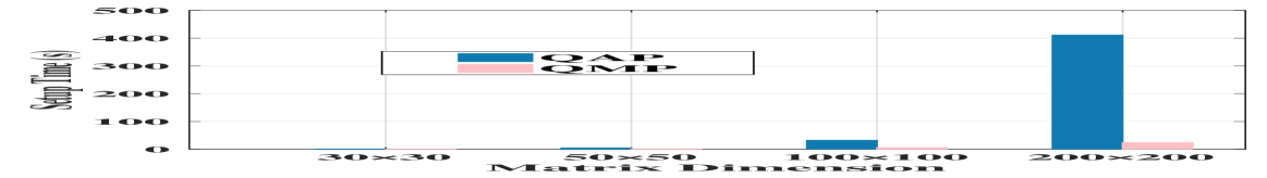
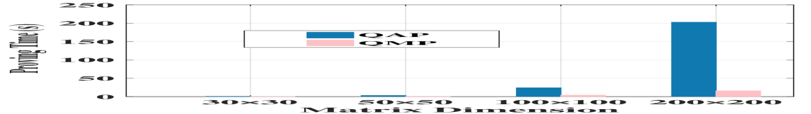
Figure 12: Comparison on Setup time and proving time.

TABLE IV: CRS size comparison (KB).

Matrix dimension	$\mathbf{30\times 30}$	$\mathbf{50\times 50}$	$\mathbf{100\times 100}$	$\mathbf{200\times 200}$
QAP	2,911.22	12,445.73	97,230.09	768,503.09
QMP	84.42	233.83	934.21	3,735.72
Matrix dimension	$\mathbf{500\times}$	$\mathbf{1000\times}$	$\mathbf{2000\times}$	$\mathbf{3000\times}$
QMP	23,346.32	93,384.16	373,535.53	840,454.47

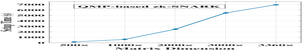
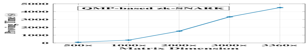
Figure 13: Performance of our QMP-based zk-SNARK handling matrix multiplication in dimensions greater than $220\times 220$.

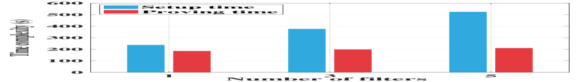
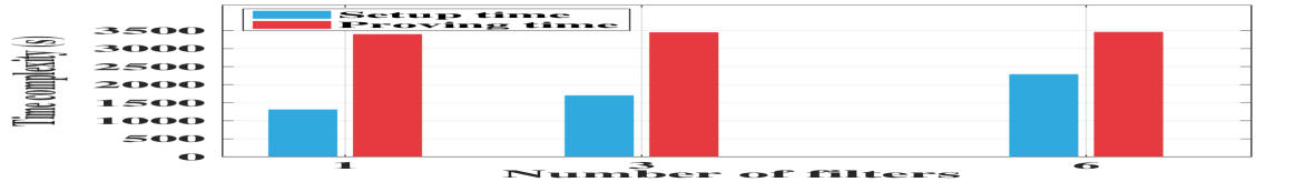
Figure 14: Setup time and proving time for a conv. layer with 1000 images from MNIST and CIFAR-10.

TABLE V: Other performance metrics.

Datasets	#Filter	Verification time (s)	Size (KB)
			CRS	Proof
MNIST	1	54559	1,054,266.00	351,421.97
	3	54002	1,054,266.00	351,421.97
	5	56011	1,054,266.00	351,421.97
CIFAR-10	1	375942	15353859056	351,421.97
	3	376144	15353859056	351,421.97
	6	408911	16927629296	351,421.97

We can see in Fig. 13 that the QMP-based zk-SNARK can handle the matrix multiplication in increasing dimensions up to $3360\times 3360$, which is its merit, compared to the QAP-based zk-SNARK supporting the maximum number of multiplication bound $10^{7}$ [14]. Also, the proving time almost increases linearly by the dimension of matrices.

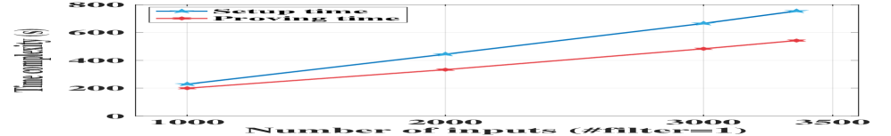
Figure 15: Time complexity on MNIST dataset.

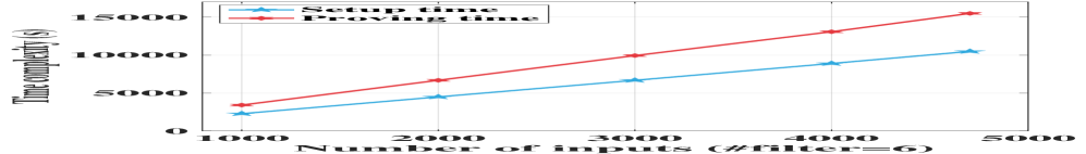
Figure 16: Time complexity on CIFAR-10 dataset.

We proceed to apply the QMP-based zk-SNARK in a convolution layer with stride $(1,1)$, taking as inputs $1000$ single-channel images of $28\times 28$ from MNIST and $1000$ three-channel images of $32\times 32$ from CIFAR-10. For the former dataset, we use $5$ filters of $5\times 5$ while for the latter one, we use $6$ filters. We transform the convolution operations into a matrix multiplication between a weight matrix and an input matrix both in dimension $3360\times 3360$ for MNIST (similarly, $4704\times 4704$ for CIFAR-10). We note $3360=28\times(28-5+1)\times 5\approx mn^{2}$, where $m,n$ mean the dimension of a filter and an image, respectively. Here, $m\geq M$ which is the number of filters. Different from the aforementioned experiments where the values of matrices are random integers, the weight matrix of $3360\times 3360$ here is strategically assigned with the weights of filters plus some zero elements as padding, for ensuring computation correctness (recall it in Fig.5), and similarly, the input matrix of $3360\times 3360$ is assigned with the pixel values of $1000$ images, padding with $3360\times(3360-1000)$ zeros. As a result, the average performance results of 5 runs are shown in Fig. 14. We discover that compared to the aforementioned experiments as presented in Fig.13, the Setup and proving time here are relatively smaller. The main reason can be the padding zero elements inside the weight and input matrices cancel a lot of multiplications. Besides the Setup and proving time, TABLE V demonstrates the corresponding verification time, as well as constant CRS size and proof size.

We further conduct additional experiments (named Exp ($\star$)) on different number of filters and an increasing number of inputs from MNIST and CIFAR-10 datasets, as elaborated in Fig. 15 and Fig. 16. We can see from the figures that the proving time basically stays stable regardless of the number of filters, but the Setup time increases linearly by the number of filters $M$. We note that the complexity of the proving time is $O(mn^{2}\cdot mn^{2}),m\geq M$ (resp. $O(Mn^{2}\cdot Mn^{2})$ if $m<M$), where $mn^{2}$ (resp. $Mn^{2}$) is the number of inputs, and the proving time is independent of the number of filters $M$.

We proceed to generate QAP-based proofs for the ReLU and average pooling operations on the $3360\times 3360$ matrix, named Exp ($\star\star$). Note that a ReLU operation needs $20$ constraints and an average pooling operation needs $144$ constraints. The evaluated performance is elaborated in TABLE VI.

TABLE VI: Performance for Exp ($\star\star$) (s).

Layer	Setup Time	Proving Time	Verification Time
ReLU	5520.61	1448.83	14.78
Pooling	196.43	49.93	14.78

VIII Conclusion

The paper discusses using zk-SNARK systems for verifiable CNN testing on encrypted test data. The authors optimize matrix multiplication relations by representing convolution operations with a single MM computation and using a new QMP. This reduces the multiplication gate and proof generation overhead. They also aggregate multiple proofs into a single proof for the same CNN but different test datasets. They provide a proof-of-concept implementation and share their implementation code publicly.

VIII-A Discussion

In terms of verification time and proof size, the QMP-based zk-SNARK has a higher overhead than the QAP-zk-SNARK. Its verification time grows faster than that of QAP-based zk-SNARK, see TABLE VIII. The proof size also becomes lager when the matrix dimension turns lager as shown in TABLE VII, while the proof size in the QAP-based zk-SNARK keeps $1019~{}$bits regardless of the matrix dimension. We next see how the proof size becomes longer with the matrix dimension increasing. We note that the bounded number of multiplications the QAP zk-SNARK can handle is $220*220*220=10,648,000$, and then the QAP zk-SNARK would be called multiple times when handling the multiplication operations more than $10,648,000$, which results in multiple $1019$-bit proofs. Suppose that the QAP-based zk-SNARK proofs for the $3000\times 3000$ matrix multiplication are totally $\frac{3000*3000*3000}{220*220*220}$ $\times 1019$ bits. Also, the QMP-based zk-SNARK proofs for the same matrix multiplication are $2,295,000,764$ bits. The proof size is nearly $888$ times larger than that of the above QAP-based zk-SNARK proof. We observe that the times of magnitude become smaller as the matrix dimension increases, see TABLE VII, which may mean that the QMP-based zk-SNARK is more suitable to handle large matrix multiplication.

TABLE VII: Times of magnitude in proof size.

Matrix dimension	$\mathbf{1000\times}$	$\mathbf{2000\times}$	$\mathbf{3000\times}$	$\mathbf{3360\times}$	$\mathbf{4000\times}$
Times	2665	1332	888	793	666

TABLE VIII: Verification time comparison (s).

Matrix dimension	$\mathbf{30\times 30}$	$\mathbf{50\times 50}$	$\mathbf{100\times 100}$	$\mathbf{200\times 200}$
QAP	0.005	0.007	0.014	0.044
QMP	4.896	13.580	54.630	215.800

In our future work, we would introduce a random sampling strategy in the phase of proof generation, aiming to reduce the verification time. A straightforward idea can be adopted by randomly sampling a bounded number of values in two matrices to be multiplied, and resetting the non-chosen values as zeros. In such a way, only the sampled values in the two matrices are multiplied and only their multiplication correctness need to be proved. But here two noteworthy issues should be considered: (1) how to generate the randomness used for sampling against a distrusted prover; (2) how to determine the bound of the number of sampled values for ensuring computational soundness in zk-SNARK.

References

• [1] Y. LeCun, B. Boser et al., “Backpropagation applied to handwritten zip code recognition,” Neural computation, vol. 1, no. 4, pp. 541–551, 1989.
• [2] R. Das, E. Piciucco et al., “Convolutional neural network for finger-vein-based biometric identification,” IEEE Transactions on Information Forensics and Security, vol. 14, no. 2, pp. 360–373, 2018.
• [3] G. Accident, “A google self-driving car caused a crash for the first time.” https://www.theverge.com/2016/2/29/11134344/google-self-driving-car-crash-report, 2016.
• [4] “The two-year fight to stop amazon from selling face recognition to the police.” https://www.technologyreview.com/2020/06/12/1003482/amazon-stopped-selling-police-face-recognition-fight/, 2020.
• [5] M. Wicker, X. Huang et al., “Feature-guided black-box safety testing of deep neural networks,” in Proc. of TACAS, 2018.
• [6] A. Aggarwal, S. Shaikh, S. Hans, S. Haldar, R. Ananthanarayanan, and D. Saha, “Testing framework for black-box ai models,” in Proc. of IEEE/ACM ICSE-Companion, 2021.
• [7] L. Ma, F. Juefei-Xu et al., “Deepgauge: Multi-granularity testing criteria for deep learning systems,” in Proc. of ACM/IEEE ICASE, 2018.
• [8] D. Hendrycks and T. Dietterich, “Benchmarking neural network robustness to common corruptions and perturbations,” in ICLR, 2018.
• [9] L. Aroyo and P. Paritosh, “Uncovering unknown unknowns in machine learning,” https://ai.googleblog.com/2021/02/uncovering-unknown-unknowns-in-machine.html, 2021.
• [10] Z. Ghodsi, T. Gu, and S. Garg, “Safetynets: Verifiable execution of deep neural networks on an untrusted cloud,” in Proc. of NIPS, 2017.
• [11] M. I. M. Collantes et al., “Safetpu: A verifiably secure hardware accelerator for deep neural networks,” in Proc. Of IEEE VTS, 2020.
• [12] S. Lee, H. Ko, J. Kim, and H. Oh, “vcnn: Verifiable convolutional neural network.” https://eprint.iacr.org/2020/584.pdf, 2020.
• [13] B. Feng, L. Qin, Z. Zhang, Y. Ding, and S. Chu, “Zen: An optimizing compiler for verifiable, zero-knowledge neural network inferences,” https://eprint.iacr.org/2021/087.pdf, 2021.
• [14] J. Keuffer, R. Molva, and H. Chabanne, “Efficient proof composition for verifiable computation,” in Proc. of ESORICS, 2018.
• [15] L. Zhao, Q. Wang et al., “Veriml: Enabling integrity assurances and fair payments for machine learning as a service,” IEEE Transactions on Parallel and Distributed Systems, vol. 32, no. 10, pp. 2524–2540, 2021.
• [16] A. Madi, R. Sirdey et al., “Computing neural networks with homomorphic encryption and verifiable computing,” in ACNS Workshops, 2020.
• [17] T. Liu, X. Xie et al., “zkcnn: Zero knowledge proofs for convolutional neural network predictions and accuracy,” in Proc. of ACM CCS, 2021.
• [18] J. Thaler, “Time-optimal interactive proofs for circuit evaluation,” in Annual Cryptology Conference, 2013, pp. 71–89.
• [19] J. Groth, “On the size of pairing-based non-interactive arguments,” in EUROCRYPT, 2016, pp. 305–326.
• [20] S. Agrawal, C. Ganesh et al., “Non-interactive zero-knowledge proofs for composite statements,” in CRYPTO, 2018, pp. 643–673.
• [21] M. Campanelli et al., “Legosnark: Modular design and composition of succinct zero-knowledge proofs,” in Proc. of ACM CCS, 2019.
• [22] D. Fiore, A. Nitulescu, and D. Pointcheval, “Boosting verifiable computation on encrypted data,” in PKC, no. 12111, 2020, pp. 124–154.
• [23] D. Mouris and N. G. Tsoutsos, “Zilch: A framework for deploying transparent zero-knowledge proofs,” IEEE Transactions on Information Forensics and Security, 2021.
• [24] “Bvlc/caffe,” https://github.com/BVLC/caffe/wiki/Model-Zoo, 2019.
• [25] Kaggle, “Data science competition platform.” https://www.kaggle.com/.
• [26] A. Marketplace, “Machine learning solutions.” https://aws.amazon.com/marketplace/solutions/machine-learning.
• [27] G. Xu et al., “Verifynet: Secure and verifiable federated learning,” IEEE Transactions on Information Forensics and Security, vol. 15, pp. 911–926, 2019.
• [28] Z. He, T. Zhang, and R. B. Lee, “Model inversion attacks against collaborative inference,” in Proc. of ACM ACSAC, 2019.
• [29] T. Ryffel, E. Dufour-Sans et al., “Partially encrypted machine learning using functional encryption,” in NIPS, 2019.
• [30] Y. Aono, T. Hayashi et al., “Privacy-preserving deep learning via additively homomorphic encryption,” IEEE Transactions on Information Forensics and Security, vol. 13, no. 5, pp. 1333–1345, 2017.
• [31] S. G. Francesco Alesiani, “Method for verifying information,” https://patentimages.storage.googleapis.com/53/3c/62/0ed0b3f9bb163f/US20210091953A1.pdf, 2021.
• [32] N. Gailly, M. Maller, and A. Nitulescu, “Snarkpack: Practical snark aggregation.” in Proc. of RWC, 2022.
• [33] J. Zhang, T. Liu et al., “Doubly efficient interactive proofs for general arithmetic circuits with linear prover time,” in Proc. of ACM CCS, 2021.
• [34] S. Goldwasser et al., “Delegating computation: interactive proofs for muggles,” Journal of the ACM, vol. 62, no. 4, pp. 1–64, 2015.
• [35] C. Niu, F. Wu, S. Tang, S. Ma, and G. Chen, “Toward verifiable and privacy preserving machine learning prediction,” IEEE Transactions on Dependable and Secure Computing, 2020.
• [36] J. Zhang, Z. Fang et al., “Zero knowledge proofs for decision tree predictions and accuracy,” in Proc. of ACM CCS, 2020.
• [37] C. Weng, K. Yang, X. Xie, J. Katz, and X. Wang, “Mystique: Efficient conversions for zero-knowledge proofs with applications to machine learning,” in Proc. of USENIX Security, 2021, pp. 501–518.
• [38] C. Dong, J. Weng et al., “Fusion: Efficient and secure inference resilient to malicious server and curious clients,” in Proc. of NDSS, 2023.
• [39] R. Gilad-Bachrach, N. Dowlin et al., “Cryptonets: Applying neural networks to encrypted data with high throughput and accuracy,” in ICML, 2016, pp. 201–210.
• [40] P. Mohassel and Y. Zhang, “Secureml: A system for scalable privacy-preserving machine learning,” in Proc. Of IEEE S&P, 2017.
• [41] P. Mishra, R. Lehmkuhl et al., “Delphi: A cryptographic inference service for neural networks,” in USENIX Security, 2020, pp. 2505–2522.
• [42] C. Juvekar, V. Vaikuntanathan, and A. Chandrakasan, “$\{$GAZELLE$\}$: A low latency framework for secure neural network inference,” in Proc. of USENIX Security, 2018.
• [43] N. Kumar, M. Rathee et al., “Cryptflow: Secure tensorflow inference,” in IEEE S&P, 2020, pp. 336–353.
• [44] K. Huang, X. Liu et al., “A lightweight privacy-preserving cnn feature extraction framework for mobile sensing,” IEEE Transactions on Dependable and Secure Computing, vol. 18, no. 3, pp. 1441–1455, 2019.
• [45] E. Hesamifard, H. Takabi, and M. Ghasemi, “Cryptodl: Deep neural networks over encrypted data,” https://arxiv.org/abs/1711.05189, 2017.
• [46] X. Liu, R. H. Deng et al., “An efficient privacy-preserving outsourced calculation toolkit with multiple keys,” IEEE Transactions on Information Forensics and Security, vol. 11, no. 11, pp. 2401–2414, 2016.
• [47] X. Liu et al., “Efficient and privacy-preserving outsourced calculation of rational numbers,” IEEE Transactions on Dependable and Secure Computing, vol. 15, no. 1, pp. 27–39, 2016.
• [48] X. Liu, R. H. Deng et al., “Privacy-preserving outsourced calculation toolkit in the cloud,” IEEE Transactions on Dependable and Secure Computing, vol. 17, no. 5, pp. 898–911, 2018.
• [49] R. Gennaro, C. Gentry et al., “Quadratic span programs and succinct nizks without pcps,” https://eprint.iacr.org/2012/215.pdf, 2012.
• [50] J. Fan and F. Vercauteren, “Somewhat practical fully homomorphic encryption,” https://eprint.iacr.org/2012/144.pdf, 2012.
• [51] X. Chen, C. Liu et al., “Targeted backdoor attacks on deep learning systems using data poisoning,” https://arxiv.org/abs/1712.05526, 2017.
• [52] G. Xu, H. Li et al., “Secure and verifiable inference in deep neural networks,” in Proc. of ACM ACSAC, 2020.
• [53] Z. He, T. Zhang et al., “Sensitive-sample fingerprinting of deep neural networks,” in CVPR, 2019.
• [54] Y. Zhang et al., “Stealing neural network structure through remote fpga side-channel analysis,” IEEE Transactions on Information Forensics and Security, vol. 16, pp. 4377–4388, 2021.
• [55] M. Yan et al., “Cache telepathy: Leveraging shared resource attacks to learn dnn architectures,” in Proc. of USENIX Security, 2020.
• [56] G. Saileshwar et al., “Mirage: Mitigating conflict-based cache attacks with a practical fully-associative design.” in Proc. of USENIX Security, 2021.
• [57] A. E. Kosba, D. Papadopoulos et al., “Trueset: Faster verifiable set computations,” in Proc. of USENIX Security, 2014.