High-$\mathbf{Q^{2}}$ Behavior of Structure Function $\mathbf{F_{2}}$ with the Solution to Balitsky-Kovchegov Equation

Abstract

As a lot of studies have declared, the proton structure function $F_{2}$ explicitly satisfies a power-law mathematical formation. We describe the behavior of proton structure function $F_{2}$ at small-$x$ as well as large $Q^{2}$ using the analytical solution of the Balitsky-Kovchegov equation. We obtain the effective slope value $\lambda$ of the structure function with $Q^{2}$. Our results come from fitting the HERA experimental data at low $Q^{2}$ region and we also give the prediction for the effective slope of $F_{2}$ at the high $Q^{2}$ region.

I Introduction

Quantum chromodynamics (QCD) is used to explain the interactions between hadrons, especially the high-energy scattering processes. However, due to the color confinement nature of QCD, we cannot obtain pure interaction between quarks and gluons, which are crucial for high-energy physics. Fortunately, due to the asymptotic freedom of QCD Gross and Wilczek (1973); Politzer (1973), the behavior in the high energy region can be solved using perturbation theory. Experimentally, the high-energy lepton-nucleon scattering experiments of recent years have given physicists a window to study the strong interactions. Lots of hadron structure-related issues need to be considered.

In last two decades, the LO and NLO of the Balitsky-Fadin-Kuraev-Lipatov (BFKL) equation Lipatov (1976); Kuraev et al. (1977); Balitsky and Lipatov (1978) were studied by L. N. Lipatov et al. Ellis et al. (2008); Kowalski et al. (2010, 2011, 2013, 2014, 2016, 2017); Salam (1998), using the Green’s function approach. They argued that the BFKL equation shall be considered as an eigen-equation with eigenvalue $\omega_{n}$. The authors in Ref. Ellis et al. (2008) argued that the discrete asymptotically-free BFKL Pomeron has been shown firstly to describe the HERA data at low $x$ and high $Q^{2}$. Most of the Deep inelastic scattering (DIS) data provided by HERA are well described by the Dokshitzer–Gribov–Lipatov–Altarelli–Parisi (DGLAP) equations Dokshitzer (1977); Gribov and Lipatov (1972); Lipatov (1974); Altarelli and Parisi (1977) equation presented by the renormalization group evolution Wilson (1975). However, the discussion related to HEAR data for small $x$ regions was initiated with the combination of the DGLAP and BFKL equations. In other words, since the variation of the scattering cross section with energy has to satisfy the unitarity limit naturally, the BFKL as a linear evolution equation will destroy this property in the high energy region. Fortunately, the infinite growth of gluons seems to be suppressed by certain processes. The saturation behavior of gluons is discussed in Ref. Mueller (2001); Stasto et al. (2001); Munier and Peschanski (2003) (and references cited therein). Balitsky-Kovchegov (BK) equation Balitsky (1997); Kovchegov (1999, 2000); Balitsky (2001), a nonlinear equation representing the evolution of gluons, which is a mean-field approximation to the Jalilian-Marian-Iancu-McLerran-Weigert-Leonidov-Kovner (JIMWLK) equation Balitsky (1996); Jalilian-Marian et al. (1997); Iancu et al. (2001); Weigert (2002). The BK equation describes the gluon behavior in the small $x$ region. Some of us obtained the analytical solution of the BK equation at momentum space in a novel way in previous work Wang et al. (2021).

HERA collaboration provides high precision data for the proton structure function $F_{2}$, therefore, it is used to study the behavior of $F_{2}$ at the small $x$ and large $Q^{2}$ conditions. The behavior of the structure function at small $x$ region is generally understood by studying its slope parameter $\lambda$ Bartels and Kowalski (2001), with the form $\lambda\propto\partial\ln F_{2}/\partial\ln(1/x)$. A significant amount of previous works include this topic in a comprehensive manner Ellis et al. (2008); Kowalski et al. (2010, 2011, 2013, 2014, 2016, 2017); Salam (1998); Cvetic et al. (2009); Cooper-Sarkar et al. (1998); Kotikov and Parente (1999); Kotikov (2007); Ball and Forte (1994); Illarionov et al. (2008); Mankiewicz et al. (1997) (and references cited therein). Until recent years, physicists also given different explanations and fitting results with new HERA data Abramowicz et al. (2015); Luszczak and Kowalski (2020). In contrast to the range of $Q^{2}$ included in the data, several theoretical works give results for the parameter lambda versus $Q^{2}$ for only the intermediate region such as $\mathcal{O}(200)$ MeV² Kotikov and Parente (1999); Illarionov et al. (2008); Kaidalov et al. (2001); Donnachie and Landshoff (2003). Of course, the data of structure function $F_{2}$ at very high $Q^{2}$ are all for the large $x$ scale. All these considerations lead us to be interested in double-asymptotic-scaling (DAS) phenomenon, which means the limits for $Q^{2}\to\infty$ and $x\to 0$.

In present work, we associate the experiments as well as the QCD evolution theory to analyze the proton structure function from the perspective of the BK equation. Based on the form of analytic solution introduced in previous work Wang et al. (2021), we calculate the proton structure function $F_{2}$ at higher $Q^{2}$ and analyze the small $x$ behavior by fitting computed results. The organization of this paper is as follows. In Sec. II, we briefly introduce the methods and principles which of calculating the proton structure function $F_{2}$ by using analytical solution of BK equation in Ref. Wang et al. (2021). We then discuss, in Sec. III how one can get the structure function $F_{2}$ and corresponding effective slop parameter $\lambda$ in high energies. In Sec. IV we briefly discuss the interesting results from Sec. III. The summaries about this work are represented in Sec. V.

II Formalism

We consider the high-energy scattering process with the dipole model (see FIG. 1). The high-speed moving photon fluctuates the $q\bar{q}$ pair from QCD vacuum into a dipole. The total cross section of the overall $\gamma^{*}p$ scattering is represented by integrating the dipole cross section with the photon wave functions Mueller and Patel (1994); Kowalski and Teaney (2003); Kowalski et al. (2006). The momentum space formulation of the dipole scattering cross section can be obtained from the Fourier transform. If the transverse profile of the proton is considered as an isotropic disk with radius $R_{p}$, the dipole scattering cross section is considered to be proportional to the forward scattering amplitude $\mathcal{N}(r,Y)$ related to de Santana Amaral et al. (2007)

$$\sigma_{\mathrm{dip}}^{\gamma^{*}p}(r,Y)=2\pi R_{p}^{2}\mathcal{N}(r,Y),$$ (1)

in which $R_{p}$ is treated as the electronic radius of proton.

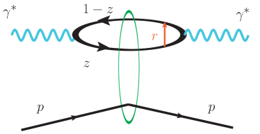
Figure 1: (color online). The elastic scattering of a virtual photon on a proton in the dipole representation Kowalski et al. (2006).

Based on the above discussions and some algebraic calculations, the structure function of proton can be expressed in momentum space as Barone and Predazzi (2002); de Santana Amaral et al. (2007)

$$\small F_{2}\left(x,Q^{2}\right)=\frac{Q^{2}R_{p}^{2}N_{c}}{4\pi^{2}}\int_{0}^{\infty}\frac{dk}{k}\int_{0}^{1}dz\left|\tilde{\Psi}\left(k^{2},z;Q^{2}\right)\right|^{2}\mathcal{N}(k,Y),$$ (2)

with the Fourier transform

$$\small\mathcal{N}(k,Y)=\frac{1}{2\pi}\int\frac{d^{2}r}{r^{2}}e^{i\mathbf{k}\cdot\mathbf{r}}\mathcal{N}(r,Y)=\int_{0}^{\infty}\frac{dr}{r}J_{0}(kr)\mathcal{N}(r,Y).$$ (3)

The photo wave functions $\tilde{\Psi}$ in Eq. (2) can be found in Ref. de Santana Amaral et al. (2007) in the momentum space. Of course, not only DIS calculations, but also the vector meson diffractive production process has a similar wave function representation to calculate Kowalski et al. (2006); Xie and Chen (2018). Now we shall handle the forward scattering amplitude by the method from Wang et al. (2021). The BK equation is rewritten as the Fisher-KPP equation FISHER (1937) with some variable substitution. We use the analytical solution of BK equation calculated by Homogeneous Balance method in Refs. Wang (1995, 1996); Zhou et al. (2003, 2004); Wang and Li (2014), thus it is expressed as Wang et al. (2021)

$$\mathcal{N}(L,Y)=\frac{A_{0}e^{5A_{0}Y/3}}{\left[e^{5A_{0}Y/6}+e^{\left[-\theta+\sqrt{A_{0}/6A_{2}}\left(L-A_{1}Y\right)\right]}\right]^{2}},$$ (4)

where the variable $L=\ln\left(k^{2}/k_{0}^{2}\right)$ with the cutoff $k_{0}=\Lambda_{\mathrm{QCD}}=200$ MeV. The parameter values $\theta$, $A_{0}$, $A_{1}$, $A_{2}$ are referred to Marquet and Soyez (2005); Wang et al. (2021), which can be obtained by fitting experimental data.

In accordance with all the discussions in this section, we shall relate the structure function $F_{2}$ of the proton to solution Eq. (4) of the BK equation with reference to the QCD evolution behaviors. We discuss the analysis process in detail is as following sections.

III Structure function $\mathbf{F_{2}(x,Q^{2})}$ in High energies

In Ref. de Santana Amaral et al. (2007), the authors already discussed in detail the process of calculating the structure function $F_{2}$, including the selection of parameters contained in the momentum space photon wave function. We use the same formalism from Ref. de Santana Amaral et al. (2007) to get several parameters in the analytical solution of the BK equation by fitting HERA data Andreev et al. (2014); Abramowicz et al. (2015). Considering the small $x$ limit, we chose to fit the experimental data in the range of 2.5 GeV${}^{2}<Q^{2}<$250 GeV², because the amount of data as well as the precision in this region are appropriate.

According to the discussions from Wang et al. (2021), we fixed the strong coupling constant $\bar{\alpha_{\mathrm{s}}}\equiv\alpha_{\mathrm{s}}N_{c}/\pi=0.191$. It is effective in the energy range we considered. In order to calculate $F_{2}$ with Eq. (2), the color number $N_{c}$ is determined to $3$, and the considerations of quark mass and flavor are not changed which we used in Ref. de Santana Amaral et al. (2007). In other words, we choose $m_{u}=m_{d}=m_{q}=140$ MeV, $m_{c}=1.3$ GeV for quarks mass de Santana Amaral et al. (2007), proton size is treated as the electronic radius $R_{p}=4.23$ GeV^-1. Based on these fixed parameters options, we shall use the HERA data to fit and obtain the parameters in Eq. (4). The fitting results are displayed in FIG. 2 (with partial fitting results) and the fitting parameters of Eq. (4) are determined as $A_{0}=0.5262\pm 0.0024$, $A_{1}=1.4383\pm 0.0133$, $A_{2}=0.1047\pm 0.0008$ and $\theta=-0.4572\pm 0.0110$.

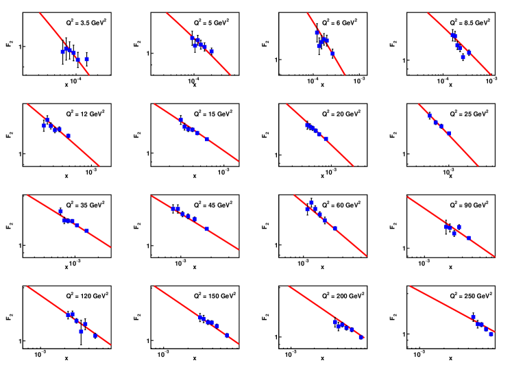
Figure 2: (color online). $x$ dependence of structure function $F_{2}(x,Q^{2})$ with bins of $Q^{2}$. The data from H1 Andreev et al. (2014) (blue squares) are compared with our fit by analytical solution of BK Wang et al. (2021) (red lines). The parameters determination is discussed in text.

Due to all the constraints of the experiment, one is often interested in the physics at the energy limit, such as $x\to 0$ and $Q^{2}\to\infty$. This research we discussed is always more mathematical, but it is usually possible to give some interesting predictions we want. We wish to investigate the small-$x$ behavior of $F_{2}$ at higher $Q^{2}$. We can find the slope parameter $\lambda\propto\partial\ln F_{2}/\partial\ln(1/x)$ at different $Q^{2}$ in Ref. Cvetic et al. (2009). At small-$x$ range ($x<0.01$), the structure function of proton $F_{2}$ can be parameterized as a power like form

$$F_{2}\left(x,Q^{2}\right)=Cx^{-\lambda\left(Q^{2}\right)}.$$ (5)

According to our calculations, the slope parameter $\lambda$ is determined from computed $F_{2}(x,Q^{2})$ by using BK equation and dipole amplitude, with Eqs. (2) and (4). This will be discussed in the next section.

IV Results and discussions

The BK equation, as a QCD theory, has some predictive power at limit conditions. Previous works have made theoretical predictions based on experimental data with proper assumptions, which are very effective and inspiring. We take this a step further by extending both the Bjorken scale $x$ and $Q^{2}$ to the limit, taking advantage of the analytical solution of the BK equation. As we discussed, we want to see what characterizes the behavior of $F_{2}$ under very high-$Q^{2}$. We shall easily extend $F_{2}$ to $Q^{2}\sim\mathcal{O}(2000)$ GeV² by just doing some numerical calculations ($2.0\times 10^{-5}<x<1.0\times 10^{-2}$). Based on the analytical solution (4) with the fitted parameters, the behavior of slope factor $\lambda$ are shown in FIG. 3.

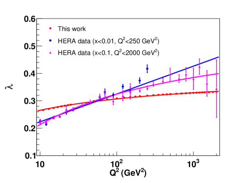
Figure 3: (color online). Slope parameter $\lambda$ v.s. energy scale $Q^{2}$ . The red squares with error bar represent our calculations, determined by Eqs. (2), (4) and (5). The Blue circles denote the extracted $\lambda$ from Abramowicz et al. (2015); Luszczak and Kowalski (2020) ($x<0.01$, $Q^{2}<250$ GeV²) and magenta triangles are extracted from same data from HREA Abramowicz et al. (2015) ($x<0.1$, $Q^{2}<2000$ GeV²). Red line represents the fitting result comes from Eq. (6) which describe the red points. The blue and magenta lines are fitting results of the corresponding color points respectively.

Figure. 3 presents the $\lambda$ values extracted from the HERA data (blue and magenta points) Andreev et al. (2014); Abramowicz et al. (2015) and our calculated results using BK equation (red solid squares), we also give parameterized formulas to describe the $\lambda-Q^{2}$ relation, which are written as

$$\lambda(Q^{2})=a(1-\frac{b}{\ln(Q^{2}/\Lambda_{\mathrm{QCD}}^{2})})+c,$$ (6)

for red and magenta points in FIG. 3 and

$$\lambda(Q^{2})=A\ln\left(\frac{Q^{2}}{\Lambda_{\mathrm{QCD}}^{2}}\right)+B,$$ (7)

for blue points Luszczak and Kowalski (2020), in which the QCD cutoff $\Lambda_{\mathrm{QCD}}=200$ MeV is fixed. We use Eq. (6) to fit our calculations and HERA data Abramowicz et al. (2015) (magenta triangles, $Q^{2}<2000$ GeV²). All parameter information is listed in TABLE. I. TABLE. II and III, respectively.

Let us consider this formula, in contrast to the logarithmic growth of $\lambda$ with $Q^{2}$ considered in other works Kaidalov et al. (2001); Donnachie and Landshoff (2003), we find that the $\lambda$ growth rate decreases slowly with increasing $Q^{2}$ because of $\mathrm{d}\lambda/\mathrm{d}Q^{2}|_{Q^{2}\to\infty}=0$. It looks like the behavior of the running strong coupling constant in the extreme of high energy (see Ref. Schrempp (2005) and references cited therein). From Eq. (6), we consider a case where $Q^{2}$ approaches infinity. At this time $\lambda$ barely grows with $Q^{2}$ and the value is taken at $\lambda(Q^{2}\to\infty)=a+c\simeq 0.41\pm 0.01$. It is probably the limit of the value that $\lambda$ will reach. The “frozen” $\lambda$ means no change even if $Q^{2}$ continues to rise, and the rates of variation of $x$ dependence of $F_{2}$ are fixed, too. We also consider the selection of the fitting range of $F_{2}$ in the limit $Q^{2}$ and found no differences ($C$ and $\lambda$ in Eq. (5)) between $x<0.01$ and $x<0.001$ we selected under this condition.

In order to explain the “frozen” $\lambda$, we consider the behavior of gluons in high-energy $\gamma^{*}p$ scattering by using the BK equation. The parameter $\lambda$ as the power index part represents the gluon emissions per unit of rapidity from high speed dipole Bartels and Kowalski (2001); Luszczak and Kowalski (2020), because of the formation of structure function is written as Ellis et al. (2008); Kowalski et al. (2010)

$$F_{2}\left(x,Q^{2}\right)=\int_{x}^{1}dz\int\frac{dk}{k}\Phi_{\text{DIS }}(z,Q,k)xg\left(\frac{x}{z},k\right),$$ (8)

where $xg\left(\frac{x}{z},k\right)$ denotes the unintegrated gluon density defined from Ellis et al. (2008), expressing as a power law form with index $\lambda$ (or eigenvalue of BFKL $\omega_{n}$). On one hand, the invariant $\lambda$ in high $Q^{2}$ region also indicates that the gluon emission rate achieves at equilibrium. The $\lambda$’s behavior we obtained is also generally consistent with the discussions and results in previous works Martin et al. (1996); Golec-Biernat and Wusthoff (1998, 1999). On the other hand, with increasing $Q^{2}$ and decreasing $x$ Luszczak and Kowalski (2020), the phase space for gluon emission grows quickly with increasing, the gluons overlap with each other when the numbers of gluon is large, the phase space growth is limited and eventually achieves a particular value, which is also unitarity of the QCD theory requires.

Our results are developed on the basis of previous related works Ellis et al. (2008); Kowalski et al. (2010, 2011, 2013, 2014, 2016, 2017); Ellis et al. (2008); Kowalski et al. (2010, 2011, 2013, 2014, 2016, 2017); Salam (1998); Cvetic et al. (2009); Cooper-Sarkar et al. (1998); Kotikov and Parente (1999); Kotikov (2007); Ball and Forte (1994); Illarionov et al. (2008); Mankiewicz et al. (1997), which generalize the $Q^{2}$-dependence lambda to the higher $Q^{2}$ situation. However, in this work, we have taken some approximations, such as the selection of fixed strong coupling constants. This approximation means that we shall think the calculation results more significant at some particular $Q^{2}$, while at very low or high $Q^{2}$ there will be differences (see FIG. 3). We argue that it is feasible to use the BK equation to investigate the proton structure function, although we make some approximations. Our results start from the QCD evolution theory, the BK equation has been shown to be a opening window in DIS and diffraction processes studies Mueller (2001); Stasto et al. (2001); Munier and Peschanski (2003). The problems we encountered are explained and solved in the future researches, which will be addressed by the solution of the BK equation in case of running coupling constants Marquet et al. (2005) or the numerical solution of JIMWLK equation Mäntysaari and Schenke (2018), especially DGLAP equation Ball and Forte (1994) in future.

V Summary

In this paper, on one hand, we mainly use the analytical solution of the BK equation from Ref. Wang et al. (2021) to calculate the proton structure function $F_{2}$ at the higher $Q^{2}$ and discuss the behaviors of structure function in the small-$x$ region. We find that the speed of growth of $\lambda$, the slope parameter of $F_{2}$, decreases as $Q^{2}$ increases. It eventually maybe converges to a certain value, precisely around $\lambda\simeq 0.41\pm 0.01$, of course, it requires large $Q^{2}$ scale. On the other hand, we present some phenomenological discussions of the results. In our views, we think gluons overlap and phase space growth supression at high scale could explain the behavior of parameter $\lambda$. The conclusion will definitely need to be tested by future high-precision Electron-Ion Collision experiments Accardi et al. (2016); Abdul Khalek et al. (2021); Chen (2018); Chen et al. (2020); Anderle et al. (2021) in wide ranges of $Q^{2}$ and $x$.

Table 1: Parameters determination according to Eq. (6) and (7), using our calculations and HERA data. The results of the last two lines come from Refs. Abramowicz et al. (2015); Luszczak and Kowalski (2020).

Parameters	$\Lambda_{\mathrm{QCD}}$ (MeV)	$a$	$b$	$c$	$A$	$B$
This work	200	$0.162\pm 0.006$	$4.800\pm 0.168$	$0.244\pm 0.006$
Fits from Luszczak and Kowalski (2020)	200				$0.044\pm 0.001$	$-0.020\pm 0.004$
Fits from Abramowicz et al. (2015)	200	$0.195\pm 0.017$	$10.657\pm 0.838$	$0.395\pm 0.016$

Table 2: The results for the $\lambda$ constant obtained from the fits of the function (5) from Ref. Luszczak and Kowalski (2020) ($x<0.01$), $Q^{2}<250$ GeV².

$Q^{2}$ (GeV2)	$\lambda$	$\delta\lambda$
0.35	0.110	0.008
0.4	0.082	0.009
0.5	0.100	0.009
0.65	0.121	0.011
0.85	0.150	0.014
1.2	0.133	0.013
1.5	0.142	0.009
2	0.159	0.007
2.7	0.169	0.005
3.5	0.173	0.004
4.5	0.189	0.004
6.5	0.200	0.003
8.5	0.208	0.004
10	0.226	0.007
12	0.215	0.005
15	0.237	0.003
18	0.242	0.003
22	0.258	0.007
27	0.267	0.004
35	0.280	0.003
45	0.292	0.004
60	0.313	0.005
70	0.332	0.009
90	0.321	0.007
120	0.352	0.008
150	0.339	0.011
200	0.373	0.010
250	0.417	0.014

Table 3: The results for the $\lambda$ constant obtained from the fits of the function (5) from Ref. Abramowicz et al. (2015) ($x<0.1$, $Q^{2}<2000$ GeV²).

$Q^{2}$ (GeV2)	$\lambda$	$\delta\lambda$
10	0.224	0.008
12	0.223	0.006
15	0.240	0.004
18	0.244	0.005
22	0.269	0.012
27	0.271	0.005
35	0.284	0.006
45	0.296	0.007
60	0.316	0.008
70	0.330	0.014
90	0.299	0.013
120	0.319	0.019
150	0.334	0.0281
200	0.339	0.006
250	0.347	0.007
300	0.361	0.008
400	0.373	0.010
500	0.396	0.023
650	0.381	0.014
800	0.397	0.025
1000	0.380	0.039
1200	0.425	0.028
1500	0.364	0.047
2000	0.345	0.105