The Forward-Backward Envelope for Sampling
with the Overdamped Langevin Algorithm

Abstract

In this paper, we analyse a proximal method based on the idea of forward-backward splitting for sampling from distributions with densities that are not necessarily smooth. In particular, we study the non-asymptotic properties of the Euler-Maruyama discretization of the Langevin equation, where the forward-backward envelope is used to deal with the non-smooth part of the dynamics. An advantage of this envelope, when compared to widely-used Moreu-Yoshida one and the MYULA algorithm, is that it maintains the MAP estimator of the original non-smooth distribution. We also study a number of numerical experiments that support our theoretical findings.

1 Introduction

The problem of calculating expectations with respect to a probability distribution $\mathfrak{p}$ in $\mathbb{R}^{d}$ is ubiquitous throughout applied mathematics, statistics, molecular dynamics, statistical physics and other fields. In practice, often $d$ is large, which renders deterministic techniques, such as quadrature methods, computationally intractable. In contrast, probabilistic methods do not suffer from the curse of dimensionality and are often the method of choice when the dimension $d$ is large. In particular, Markov chain Monte Carlo (MCMC) methods are based on the construction of a Markov chain in $\mathbb{R}^{m}$ with $m\geq d$, for which the invariant distribution (or its suitable marginal) coincides with the target distribution $\mathfrak{p}$ [1].

Often, such Markov chains are based on the discretization of stochastic differential equations (SDEs). One such SDE, which is also the focus of this paper, is the (overdamped) Langevin equation

$$\operatorname{d}X_{t}=-\nabla f(X_{t})\operatorname{d}t+\sqrt{2}\operatorname{d}W_{t},$$ (1)

where $\{W_{t}\}_{t}$ is the standard $d$-dimensional Brownian motion and $\nabla f$ denotes the gradient of a continuously-differentiable function $f:\mathbb{R}^{d}\rightarrow\mathbb{R}$. Under mild assumptions on $f$, the dynamics of (1) are ergodic with respect to the distribution $\mathfrak{p}\propto e^{-f}$. In particular, $\mathfrak{p}$ is the invariant distribution of (1) [2].

The discretization of (1), however, requires special care, since the resulting discrete Markov chain might not be ergodic [3]. In addition, even if ergodic, the resulting discrete Markov chain often has a different invariant distribution than $\mathfrak{p}$, known as the numerical invariant distribution $\widehat{\mathfrak{p}}$. The study of the asymptotic error between the numerical invariant distribution $\widehat{\mathfrak{p}}$ and the target distribution $\mathfrak{p}$ has received considerable attention recently [4, 5]. In particular, [4] investigated the effect of discretization on the convergence of the ergodic averages, and [5] presented general order conditions to ensure that the numerical invariant distribution accurately approximates the target distribution.

Another active line of research quantifies the nonasymptotic error between the numerical invariant distribution $\widehat{\mathfrak{p}}$ and the target distribution $\mathfrak{p}$. In particular, when $\mathfrak{p}$ is a smooth and strongly log-concave distribution, [6] established non-asymptotic bounds in total variation distance for the Euler-Maruyama discretization of (1), commonly known as the unadjusted Langevin algorithm (ULA). These results have also been extended to the Wasserstein distance $\mathrm{W}_{2}$ in [7, 8, 9, 10, 11], to name a few. Typically, these works study the number of iterations that the numerical integrator would require to achieve a desired accuracy, when applied to a target distribution $\mathfrak{p}$ with a known condition number.

In fact, the above strong log-concavity of $\mathfrak{p}$ can be substantially relaxed. In particular, using a variant of the reflection coupling, the recent work [12] derived non-asymptotic bounds for the ULA in the Wasserstein distance $\mathrm{W}_{1}$, when $\mathfrak{p}$ is strictly log-concave outside of a ball in $\mathbb{R}^{d}$. Similar results for the Wasserstein distance $\mathrm{W}_{2}$ have also been presented in [13].

Within the class of log-concave distributions, a significant challenge for the Langevin diffusion in (1) arises when the target distribution $\mathfrak{p}$ is not smooth and/or has a compact (convex) support in $\mathbb{R}^{d}$. One approach to address this challenge is to replace the non-smooth distribution $\mathfrak{p}$ with a smooth proxy obtained via the so-called Moreu-Yoshida (MY) envelope. This new smooth density remains log-concave and, hence, amenable to the non-asymptotic results discussed earlier. When the support of $\mathfrak{p}$ is also compact, proximal Monte Carlo methods have been explored in [14, 15, 16]. It is also worth noting that [17] pursued a different approach for sampling from compactly-supported densities that does not involve the MY envelope.

A potential drawback of the above approach is that the MY envelope often does not maintain the maximum a posteriori (MAP) estimator. That is, the above approach alters the location at which the new (smooth) density reaches its maximum. This is a well-known issue in the context of (non-smooth) convex optimization and is often resolved by appealing to the proximal gradient method. The latter can be understood as the Euler discretization of the so-called forward-backward (FB) envelope [18].

Contributions.

This work explores and analyzes the use of the FB envelope for sampling from non-smooth and compactly-supported log-concave distributions. In analogy with the Langevin proximal Monte Carlo, we replace the non-smooth density with a smooth proxy obtained via the FB envelope. In particular, this proxy is strongly log-concave over long distances.

Crucially, the new proxy also maintains the MAP estimator , under certain assumptions. However, this improvement comes at the cost of requiring additional smoothness for the smooth part of the density. Lastly, the strong convexity of the new proxy over long distances allows us to utilise the work of [12] to obtain non-asymptotic guarantees for our method in the Wasserstein distance $\mathrm{W}_{1}$.

In addition to investigating the use of FB envelope in sampling, this work has the following contributions:

• It introduces a general theoretical framework for sampling from non-smooth densities by introducing the notion of admissible envelopes. MY and FB envelopes are both instances of admissible envelopes.

• It proposes a new Langevin algorithm to sample from non-smooth densities, dubbed EULA, which generalizes MYULA. EULA can work with any admissible envelope (e.g., MY or FB) and can handle a family of increasingly more accurate envelopes rather than a fixed envelope.

Organization.

The rest of the paper is organised as follows. Section 2 formalizes the problem of sampling from a non-smooth and compactly-supported log-concave distribution. As a proxy for this non-smooth distribution, its (smooth) Moreau-Yosida (MY) envelope is reviewed in Section 3. This section also explains the main limitation of MY envelope, i.e., its inaccurate MAP estimation. In Section 4, we introduce the forward-backward (FB) envelope which overcomes the key shortcoming of the MY envelope.

Section 5 introduces and analyses EULA, an extension of the popular ULA for sampling from a non-smooth distribution. EULA can be adapted to various envelopes. In particular, MYULA from [14] is a special case of EULA for the MY envelope. Section 6 proves the iteration complexity of EULA and Section 7 presents a few numerical examples to support the theory developed here.

2 Statement of the Problem

Consider a compact convex set $\mathrm{K}\subset\mathbb{R}^{d}$. For a pair of functions $\overline{f}:\mathbb{R}^{d}\rightarrow\mathbb{R}$ and $\overline{g}:\mathbb{R}^{d}\rightarrow\mathbb{R}$, our objective in this work is to sample from the probability distribution

$$\mathfrak{p}(x):=\begin{cases}\frac{e^{-\overline{f}(x)-\overline{g}(x)}}{\int_{\mathrm{K}}e^{-\overline{f}(z)-\overline{g}(z)}\,\operatorname{d}z}&x\in\mathrm{K}\\ 0&x\notin\mathrm{K},\end{cases}$$ (2)

whenever the ratio above is well-defined. In order to sample from $\mathfrak{p}$, we only have access to the gradient of $\overline{f}$ and the proximal operator for $\overline{g}$, to be defined later. Our assumptions on $\mathrm{K},\overline{f},\overline{g}$ are detailed below.

Assumption 2.1.

We make the following assumptions:

1. For radii $R\geq r>0$, assume that $\mathrm{K}\subset\mathbb{R}^{d}$ is a compact convex body that satisfies $\mathrm{B}(0,r)\subset\mathrm{K}\subset\mathrm{B}(0,R)$. Here, $\mathrm{B}(0,r)$ is the Euclidean ball of radius $r$ centered at the origin.

2. Assume also that $\overline{f}:\mathbb{R}^{d}\rightarrow\mathbb{R}$ is a convex function that is three-times continuously differentiable.

3. Assume lastly that $\overline{g}:\mathbb{R}^{d}\rightarrow(-\infty,\infty]$ is a proper closed convex function. Moreover, we assume that $\overline{g}$ is continuous.

A few important remarks about Assumption 2.1 are in order. First, in the special case when $\overline{f}$ is a convex quadratic [20], the assumption of thrice-differentiability above is trivially met and some of the developments below are simplified. However, our more general setup here necessitates the thrice-differentiability above and results below in more involved technical derivations.

Second, instead of the two functions $\overline{f},\overline{g}$, it will be more convenient to work with two new functions $f,g$, without any loss of generality. More specifically, consider a convex function $f$ that coincides with $\overline{f}$ on the set $\mathrm{K}$, has a compact support and a continuously differentiable Hessian.

For this function $f$, the compactness of $\mathrm{K}$ and smoothness of $\overline{f}$ in Assumption 2.1 together imply that $f,\nabla f,\nabla^{2}f$ are all Lipschitz-continuous functions. To summarize, for the function $f$ described above, there exist nonnegative constants $\lambda_{0},\lambda_{1},\lambda_{2},\lambda_{3}$ such that

$$f(x)=0,\qquad\text{if }\|x\|_{2}\geq\lambda_{0},$$ (3a)

$$|f(x)-f(y)|\leq\lambda_{1}\|x-y\|_{2},\qquad x,y\in\mathbb{R}^{d},$$ (3b)

$$\|\nabla f(x)-\nabla f(y)\|_{2}\leq\lambda_{2}\|x-y\|_{2},\qquad x,y\in\mathbb{R}^{d},$$ (3c)

$$\|\nabla^{2}f(x)-\nabla^{2}f(y)\|\leq\lambda_{3}\|x-y\|_{2},\qquad x,y\in\mathbb{R}^{d}.$$ (3d)

Let us also define the proper closed convex function

$$g:=\overline{g}+1_{\mathrm{K}},$$ (4)

where $1_{\mathrm{K}}$ is the indicator function for the set $\mathrm{K}$. That is, $1_{\mathrm{K}}(x)=0$ if $x\in\mathrm{K}$ and $1_{\mathrm{K}}(x)=\infty$ if $x\notin\mathrm{K}$. The compactness of $\mathrm{K}$ and continuity of ${\bar{g}}$ in Assumption 2.1 together imply that $g$ is finite, when its domain is limited to the set $\mathrm{K}$. Outside of the set $\mathrm{K}$, $g$ is infinite. To summarize, the new function $g$ is lower semi-continuous and also satisfies

$$\max_{x\in\mathrm{K}}|g(x)|<\infty,\qquad g(x)=\infty,\quad\text{if }x\notin\mathrm{K}.$$ (5)

We can now revisit (2) and, using the new functions $f,g$, we rewrite the definition of $\mathfrak{p}$ as

$$\mathfrak{p}(x):=\frac{e^{-F(x)}}{\int_{\mathbb{R}^{d}}e^{-F(z)}\,\operatorname{d}z},\qquad x\in\mathbb{R}^{d},$$ (6a)

$$F(x):=\overline{f}(x)+\overline{g}(x)+1_{\mathrm{K}}(x)=f(x)+g(x),\qquad x\in\mathbb{R}^{d}.$$ (6b)

Above, $F$ is often referred to as the potential associated with $\mathfrak{p}$. The last identity above holds by construction. Indeed, on the set $\mathrm{K}$, the functions $f$ and $\overline{f}$ coincide. Likewise, on the set $\mathrm{K}$, the functions $g$ and $\overline{g}$ coincide. On the other hand, outside of the set $\mathrm{K}$, both sides of the last equality above are infinite.

In view of (6b), we will often use $f$ and $\overline{f}$ interchangeably throughout this work, depending on the context. Likewise, we will use $g$ and $\overline{g}$ interchangeably. Note also that the integral in the denominator above is finite by Assumption 2.1. When there is no confusion, we will overload our notation and use $\mathfrak{p}$ to also denote the probability measure associated with the law $\mathfrak{p}$.

Since $g$ is not differentiable, $F$ in (6b) is itself non-differentiable. In turn, this means that one cannot use gradient based algorithms such as ULA to sample from $\mathfrak{p}\propto e^{-F}$ [10]. One way to deal with this issue is to replace $F$ with a smooth function $F_{\gamma}$, which we will refer to as an envelope, to which we can then apply ULA. It is reasonable to require this envelope $F_{\gamma}$ to fulfill the following admissibility assumptions.

Definition 2.2 (Admissible envelopes).

For $\gamma^{0}>0$, the functions $\{F_{\gamma}:\mathbb{R}^{d}\rightarrow[-\infty,\infty]:\gamma\in(0,\gamma^{0})\}$ are admissible envelopes of $F$ if

1. There exists a function $F^{0}:\mathbb{R}^{d}\rightarrow[-\infty,\infty]$ such that $e^{-F^{0}}$ is integrable, and $F_{\gamma}$ dominates $F^{0}$. That is,

   $$\int_{\mathbb{R}^{d}}e^{-F^{0}(z)}\,\operatorname{d}z<\infty,\qquad F_{\gamma}(x)\geq F^{0}(x),\qquad x\in\mathbb{R}^{d},\,\gamma\in(0,\gamma^{0}).$$

2. $F_{\gamma}$ converges pointwise to $F$, i.e., $\lim_{\gamma\rightarrow 0}F_{\gamma}(x)=F(x)$ for every $x\in\mathbb{R}^{d}$.

3. $F_{\gamma}$ is $\lambda_{\gamma}$-smooth, i.e., there exists a constant $\lambda_{\gamma}\geq 0$ such that

   $$\|\nabla F_{\gamma}(x)-\nabla F_{\gamma}(y)\|_{2}\leq\lambda_{\gamma}\|x-y\|_{2},\qquad x,y\in\mathbb{R}^{d},\,\gamma\in(0,\gamma^{0}).$$

If $\{F_{\gamma}:\gamma\in(0,\gamma^{0})\}$ are admissible envelopes of $F$, we can define the corresponding probability densities

$$\mathfrak{p}_{\gamma}(x):=\frac{e^{-F_{\gamma}(x)}}{\int_{\mathbb{R}^{d}}e^{-F_{\gamma}(z)}\,\operatorname{d}z},\qquad x\in\mathbb{R}^{d},\,\gamma\in(0,\gamma^{0}).$$ (7)

Remark 2.3.

In the definition above, the property (i) implies that $\mathfrak{p}_{\gamma}$ can be normalized. This observation, combined with the property (ii), imply after an application of the dominated convergence theorem that

$$\lim_{\gamma\rightarrow 0}\mathfrak{p}_{\gamma}(x)=\mathfrak{p}(x),\qquad x\in\mathbb{R}^{d}.$$

where the probability measures $\mathfrak{p}$ and $\mathfrak{p}_{\gamma}$ are defined in (6a) and (7), respectively. That is, $\mathfrak{p}_{\gamma}$ converges weakly to $\mathfrak{p}$ in the limit of $\gamma\rightarrow 0$. (For completeness, the proof of this claim is included in the appendix.) In other words, we can use $\mathfrak{p}_{\gamma}$ as a proxy for $\mathfrak{p}$, provided that $\gamma$ is sufficiently small. Finally, as we will see shortly, the property (iii) guarantees the convergence of the ULA to an invariant distribution close to $\mathfrak{p}_{\gamma}$, provided that the step size of the ULA is small.

3 Moreau-Yosida Envelope and Its Limitation

For $\gamma>0$, let us define

$$F^{\textup{MY}}_{\gamma}(x):=f(x)+g_{\gamma}(x),\qquad x\in\mathbb{R}^{d},$$ (MY)

where

$$g_{\gamma}(x):=\min_{z\in\mathbb{R}^{d}}\left\{g(z)+\frac{1}{2\gamma}\|x-z\|_{2}^{2}\right\}$$ (8)

is the Moreau-Yosida (MY) envelope of $g$. Somewhat inaccurately, we will also refer to $F_{\gamma}^{\textup{MY}}$ as the MY envelope of $F$, to distinguish $F^{\textup{MY}}_{\gamma}$ from its newer alternatives. It is well-known that $g_{\gamma}$ is $\gamma^{-1}$-smooth and that $g_{\gamma}$ converges pointwise to $g$ in the limit of $\gamma\rightarrow 0$. These facts enable us to establish the admissibility of MY envelopes, as detailed below. All proofs are deferred to the appendices. We note that the result below closely relates to [16, Proposition 1].

Proposition 3.1 (Admissibility of MY envelopes).

Suppose that Assumption 2.1 is fulfilled. Then $\{F_{\gamma}^{\textup{MY}}:\gamma>0\}$ are admissible envelopes of $F$ in (6b). In particular, $\nabla F_{\gamma}^{\textup{MY}}$ is $(\lambda_{2}+\gamma^{-1})$-Lipschitz continuous, and given by the expression

$$\nabla F_{\gamma}^{\textup{MY}}(x)=\nabla f(x)+\frac{x-P_{\gamma g}(x)}{\gamma}\in\nabla f(x)+\partial g(P_{\gamma g}(x)),$$

$$P_{\gamma g}(x):=\operatorname*{arg\,min}_{z\in\mathbb{R}^{d}}\left\{g(z)+\frac{1}{2\gamma}\|x-z\|_{2}^{2}\right\}.$$ (9)

Above, $\lambda_{2}$ was defined in (3c), $P_{\gamma g}:\mathbb{R}^{d}\rightarrow\mathbb{R}^{d}$ is the proximal operator associated with the function $\gamma g$, and $\partial g(z)$ is the subifferential of $g$ at $z$ [21].

Remark 3.2 (Connection to Nesterov’s smoothing technique).

Alternatively, we can also view the MY envelope through the lens of Nesterov’s smoothing technique [22]. More specifically, if Assumption 2.1 is fulfilled, one can invoke a standard minimax theorem to verify that

$$g_{\gamma}(x)=\max_{z\in\mathbb{R}^{d}}\left\{\langle x,z\rangle-g^{*}(z)-\frac{\gamma}{2}\|z\|_{2}^{2}\right\},\qquad x\in\mathbb{R}^{d},$$

where $g^{*}$ is the Fenchel conjugate of $g$. The right-hand side above plays a key role in Nesterov’s technique for minimizing the non-smooth function $F$ in (6a).

In view of the admissibility of $F^{\textup{MY}}_{\gamma}$ by Proposition 3.1, applying ULA to the new potential $F^{\textup{MY}}_{\gamma}$ leads to a well-defined algorithm, see Remark 2.3. In addition, if $\gamma$ is sufficiently small, $\mathfrak{p}^{\textup{MY}}_{\gamma}\propto e^{-{F_{\gamma}^{\textup{MY}}}}$ would be close to the target distribution $\mathfrak{p}$ by Remark 2.3. This technique is known as MYULA [14]. However, a limitation of the MY envelope is that the minimizers of $F^{MY}_{\gamma}$ are not necessarily the same as the minimizers of $F$. In turn, the MAP estimator of $\mathfrak{p}_{\gamma}^{\textup{MY}}$, denoted by $x^{\textup{MY}}_{\gamma}$, might not coincide with the MAP estimator of $\mathfrak{p}$, except in the limit of $\gamma\rightarrow 0$. That is

$$\lim_{\gamma\rightarrow 0}F_{\gamma}(x_{\gamma}^{\textup{MY}})=\min_{x}F(x).$$

This observation is particularly problematic because, as we will see later, very small values of $\gamma$ are often avoided in practice due to numerical stability issues. In view of this discussion, our objective is to replace the MY envelope with a new envelope that has the same minimizers as $F$ for all sufficiently small $\gamma$, and not just in the limit of $\gamma\rightarrow 0$.

4 Forward-Backward Envelope

In this section, we will study an envelope that addresses the limitations of the MY envelope. More specifically, for $\gamma>0$, let us recall from [18] that the forward-backward (FB) envelope of the function $F$ in (6b) is defined as

$$F_{\gamma}^{\textup{FB}}(x):=f(x)-\frac{\gamma}{2}\|\nabla f(x)\|_{2}^{2}+g_{\gamma}(x-\gamma\nabla f(x)),\qquad x\in\mathbb{R}^{d},$$ (FB)

where $g_{\gamma}$ was defined in (8). A number of useful properties of $F^{\textup{FB}}_{\gamma}$ are collected below for the convenience of the reader [18]. Recall that $P_{\gamma g}$ denotes the proximal operator associated with the function $\gamma g$ in (9).

Proposition 4.1 (Properties of the FB envelope).

Suppose that Assumption 2.1 is fulfilled. For $\gamma\in(0,1/\lambda_{2})$ and every $x\in\mathbb{R}^{d}$, it holds that

1. $F(P_{\gamma g}(x-\gamma\nabla f(x))\leq F_{\gamma}^{\textup{FB}}(x)\leq F(x)$, which relates the function $F$ to its FB envelope.

2. $F_{\frac{\gamma}{1-\gamma\lambda_{2}}}^{\textup{MY}}(x)\leq F_{\gamma}^{\textup{FB}}(x)\leq F_{\gamma}^{\textup{MY}}(x)$, which relates the MY and FB envelopes of the function $F$.

3. $F_{\gamma}^{\textup{FB}}$ is continuously differentiable and its gradient is given by

   $$\nabla F_{\gamma}^{\textup{FB}}(x)=\gamma^{-1}(I-\gamma\nabla^{2}f(x))(x-P_{\gamma g}(x-\gamma\nabla f(x))).$$

4. $\operatorname*{arg\,min}F^{\textup{FB}}_{\gamma}=\operatorname*{arg\,min}F$, i.e., the function $F$ and its FB envelope have the same minimizers.

In view of Proposition 4.1(iv), a remarkable property of the FB envelope is that the modes of $\mathfrak{p}_{\gamma}^{\textup{FB}}\propto e^{-F^{\textup{FB}}_{\gamma}}$ coincide with the modes of the target measure $\mathfrak{p}\propto e^{-F}$, for all sufficiently small $\gamma$, rather than only in the limit of $\gamma\rightarrow 0$. Indeed, very small values of $\gamma$ are often avoided in practice due to numerical stability issues. This observation signifies the advantage of the FB envelope over the MY envelope. Recall that the modes of the MY envelope coincide with those of $\mathfrak{p}$ only in the limit of $\gamma\rightarrow 0$, see Section 3.

As a side note, let us remark that the proximal gradient descent algorithm for minimizing the (non-smooth) function $F$ coincides with the gradient descent (with variable metric) for minimizing the (smooth) function $F^{\textup{FB}}_{\gamma}$, whenever $\gamma$ is sufficiently small [18]. It is also easy to use Proposition 4.1 to check the admissibility of the FB envelopes, as summarized below.

Proposition 4.2 (Admissibility of FB envelopes).

Suppose that Assumption 2.1 is fulfilled. Then $\{F_{\gamma}^{\textup{FB}}:\gamma\in(0,\gamma^{\textup{FB}})\}$ are admissible envelopes of $F$ in (6b), where

$$\gamma^{\textup{FB}}:=\frac{1}{2\lambda_{2}+2\lambda_{3}(\lambda_{0}+R)}.$$ (10)

Moreover, it holds that

$$\left\|\nabla F^{\textup{FB}}_{\gamma}(x)-\nabla F^{\textup{FB}}_{\gamma}(y)\right\|_{2}\leq\lambda_{\gamma}^{\textup{FB}}\|x-y\|_{2},\qquad x,y\in\mathbb{R}^{d},$$ (11a)

$$\langle x-y,\nabla F^{\textup{FB}}_{\gamma}(x)-\nabla F^{\textup{FB}}_{\gamma}(y)\rangle\geq\mu^{\textup{FB}}_{\gamma}\|x-y\|_{2}^{2},\qquad\|x-y\|_{2}\geq\rho_{\gamma}^{\textup{FB}},$$ (11b)

where

$$\lambda^{\textup{FB}}_{\gamma} :=\gamma^{-1}+2\lambda_{2}+\lambda_{3}(\lambda_{0}+R),\quad\mu^{\textup{FB}}_{\gamma}:=\lambda_{2}+\lambda_{3}(\lambda_{0}+R),$$

$$\rho_{\gamma}^{\textup{FB}} :=\frac{2R}{1-2\gamma(\lambda_{2}+\lambda_{3}(\lambda_{0}+R)))}.$$

The equation (11) provides valuable information about the landscape of the FB envelope of $F$, which we now summarize: (11a) means that $F^{\textup{FB}}_{\gamma}$ is a $\lambda_{\gamma}^{\textup{FB}}$-smooth function. The smoothness of $F^{\textup{FB}}_{\gamma}$ in (FB) is not surprising since both $f$ and $g_{\gamma}$ are smooth functions. (Recall that $g_{\gamma}$ is the MY envelope of $g$, which is known to be $\gamma^{-1}$-smooth.)

Moreover, even though $F^{\textup{FB}}_{\gamma}$ is not necessarily a strongly convex function, (11b) implies that $F^{\textup{FB}}_{\gamma}$ behaves like a strongly convex function over long distances. As detailed in the proof, (11b) holds essentially because the MY envelope of the indicator function $1_{\mathrm{K}}$ is the function $\frac{1}{2\gamma}\operatorname{dist}(\cdot,\mathrm{K})^{2}$. The latter function grows quadratically faraway from the origin. Here, $\operatorname{dist}(\cdot,\mathrm{K})$ is the distance to the set $\mathrm{K}$.

It is worth noting that a similar result to Proposition 4.2 is implicit in [14]. That is, the MY envelope $F^{\textup{MY}}_{\gamma}$ also satisfies (11), albeit with different constants.

Remark 4.3 (Convergence in the Wasserstein metric).

Recall from Remark 2.3 that  $\mathfrak{p}_{\gamma}^{\textup{FB}}$ converges weakly to $\mathfrak{p}$ in the limit of $\gamma\rightarrow 0$. This weak convergence implies convergence in the Wasserstein metric by [23, Lemma 2.6]:

$$\lim_{\gamma\rightarrow 0}\mathrm{W}_{1}(\mathfrak{p}_{\gamma}^{\textup{FB}},\mathfrak{p})=0.$$ (12)

We recall that, for two probability measures $\mathfrak{q}_{1}$ and $\mathfrak{q}_{2}$ that satisfy $\mathbb{E}_{x\sim\mathfrak{q}_{1}}\|x\|_{2}<\infty$ and $\mathbb{E}_{y\sim\mathfrak{q}_{2}}\|y\|_{2}<\infty$, their $1$-Wasserstein or Kantorovich distance [24] is defined as

$$\mathrm{W}_{1}(\mathfrak{q}_{1},\mathfrak{q}_{2}):=\inf_{\begin{subarray}{c}x\sim\mathfrak{q}_{1}\\ y\sim\mathfrak{q}_{2}\end{subarray}}\mathbb{E}\|x-y\|_{2}.$$ (13)

With some abuse of notation, throughout this work, we will occasionally replace the probability measures with the corresponding probability distributions or random variables.

A non-asymptotic version of Remark 4.3 is presented below, which bounds the Wasserstein distance between the two probability measures $\mathfrak{p}^{\textup{FB}}_{\gamma}$ and $\mathfrak{p}$. In effect, the result below is an analogue of [14, Proposition 5] for the MY envelope. The key ingredient of their result is the Steiner’s formula for the volume of the set $\mathrm{K}+\mathrm{B}(0,t)=\{x:\operatorname{dist}(x,\mathrm{K})\leq t\}$ for every $t\geq 0$. The previous sum is in the Minkowski sense. Essentially, our proof strategy is to use Proposition 4.1(ii) to relate the FB and MY envelopes and then invoke [14, Proposition 5].

Theorem 4.4 (Wassenstein distance between $\mathfrak{p}^{\textup{FB}}_{\gamma}$ and $\mathfrak{p}$).

Suppose that Assumption 2.1 is fulfilled. For $\gamma\in(0,\gamma^{\textup{FB}})$, it holds that

$$\mathrm{W}_{1}(\mathfrak{p}_{\gamma}^{\textup{FB}},\mathfrak{p}) \leq\Cl[fcn]{dist1}+\frac{\Cl[fcn]{dist3}RI_{1}(\gamma)+\Cr{dist3}I_{2}(\gamma)+\Cl[fcn]{dist2}I_{2}(\gamma/(1-\gamma\lambda_{2}))}{\textup{vol}(\mathrm{K})+I_{1}(\gamma)}+\Cl[fcn]{dist4}$$

$$=:\Cl[fcn]{env}^{\textup{FB}}(\gamma),$$ (14)

where

$$\Cr{dist1}:=\frac{e^{2\max_{x\in\mathrm{K}}g(x)-\gamma\lambda_{2}\min_{z}f(z)}\int_{\mathrm{K}}\|x\|_{2}e^{-(1-\gamma\lambda_{2})f(x)}\,\operatorname{d}x}{\int e^{-f(x)-\frac{\operatorname{dist}(x,\mathrm{K})^{2}}{2\gamma}}\,\operatorname{d}x}$$

$$\quad-\frac{e^{\gamma\lambda_{2}\min_{z}f(z)-2\max_{x\in\mathrm{K}}g(x)}\int_{\mathrm{K}}\|x\|_{2}e^{-f(x)}\,\operatorname{d}x}{\int e^{-(1-\gamma\lambda_{2})f(x)-\frac{\operatorname{dist}(x,\mathrm{K})^{2}}{2\gamma/(1-\gamma\lambda_{2})}}\,\operatorname{d}x},$$

$$\Cr{dist3}:=e^{\max_{x}f(x)-\min_{x}f(x)},$$

$$\Cr{dist2}:=e^{\max_{x}f(x)-\min_{x}f(x)+2\max_{x\in\mathrm{K}}g(x)},$$

$$\Cr{dist4}:=e^{\max_{x\in\mathrm{K}}g(x)-\min_{x\in\mathrm{K}}g(x)}-e^{\min_{x\in\mathrm{K}}g(x)-\max_{x\in\mathrm{K}}g(x)},$$

$$I_{1}(\gamma):=\sum_{i=0}^{d-1}\textup{vol}_{i}(\mathrm{K})\cdot(2\pi\gamma)^{\frac{d-i}{2}},$$

$$I_{2}(\gamma):=\sum_{i=0}^{d-1}\textup{vol}_{i}(\mathrm{K})\cdot(2\pi\gamma)^{\frac{d-i}{2}}\left(\sqrt{\gamma(d-i+3)}+R\right).$$ (15)

Above, $\textup{vol}_{i}(\mathrm{K})$ is the $i$-th intrinsic volume of $\mathrm{K}$, see [25]. In particular, the $d$-th volume of $\mathrm{K}$ coincides with the standard volume of $\mathrm{K}$, i.e., $\textup{vol}_{d}(\mathrm{K})=\textup{vol}(\mathrm{K})$. Moreover, to keep the notation light, above we have suppressed the dependence of $\Cr{dist1}$ to $\Cr{env}^{\textup{FB}}$ on $\mathrm{K},f,g,\gamma$. As a sanity check, consider the special case of $g=1_{\mathrm{K}}$, where $1_{\mathrm{K}}$ is the indicator function for the set $\mathrm{K}$. Then we can use (15) to verify that $\Cr{dist1}$ and $I_{1}(\gamma)$ and $I_{2}(\gamma)$ and $I_{2}(\gamma/(1-\gamma\lambda_{2}))$ all vanish when we send $\gamma\rightarrow 0$. Consequently, both the left- and right-hand sides of (14) vanish if we send $\gamma\rightarrow 0$. When $g=1_{\mathrm{K}}$, then Theorem 4.4 is precisely the analogue of [14, Proposition 5]. Their work, however, does not cover the case of $g\neq 1_{\mathrm{K}}$.

In our result, when $g\neq 1_{\mathrm{K}}$ and $\gamma\rightarrow 0$, the right-hand side of (14) converges to the nonzero value

$$\left(e^{2\max_{x\in\mathrm{K}}g(x)}-e^{-2\max_{x\in\mathrm{K}}g(x)}\right)\frac{\int_{\mathrm{K}}\|x\|_{2}e^{-f(x)}\,\operatorname{d}x}{\int e^{-f(x)}\,\operatorname{d}x}$$

$$\quad+\left(\frac{e^{\max_{x\in\mathrm{K}}g(x)}}{e^{\min_{x\in\mathrm{K}}g(x)}}-\frac{e^{\min_{x\in\mathrm{K}}g(x)}}{e^{\max_{x\in\mathrm{K}}g(x)}}\right),$$

unlike the left-hand side of (14), which converges to zero by (12). Improving (14) in the case $g\neq 1_{\mathrm{K}}$ appears to require highly restrictive assumptions on $g$ which we wish to avoid here. Moreover, in practice, very small values of $\gamma$ are often avoided due to numerical stability issues. In this sense, improving (14) for very small values of $\gamma$ might have limited practical value.

To summarize this section, the FB envelopes $\{F^{\textup{FB}}_{\gamma}:\gamma\in(0,\gamma^{0,\textup{FB}})\}$ are admissible and we can use them as a differentiable proxy for the non-smooth function $F$ in (6b). Crucially, the FB envelope addresses the key limitation of the MY envelope, i.e., the modes of $\mathfrak{p}^{\textup{FB}}_{\gamma}\propto e^{-F^{\textup{FB}}_{\gamma}}$ coincide with the modes $\mathfrak{p}\propto e^{-F}$, for all sufficiently small $\gamma$, rather than only in the limit of $\gamma\rightarrow 0$.

5 EULA:
Envelope Unadjusted Langevin Algorithm

We have so far introduced two smooth envelopes for the non-smooth function $F$ in (6b), namely, the MY envelope $F^{\textup{MY}}_{\gamma}$ in (MY) and the FB envelope $F^{\textup{FB}}_{\gamma}$ in (FB). We also described in Section 4 the advantage of the FB envelope over the MY envelope. To keep our discussion general, below we consider admissible envelopes $\{F_{\gamma}:\gamma\in(0,\gamma^{0})\}$ for the target function $F$ in (6b), see Definition 2.2. Our discussion below can be specialized to either of the envelopes by setting $F_{\gamma}=F^{\textup{MY}}_{\gamma}$ or $F_{\gamma}=F^{\textup{FB}}_{\gamma}$.

For the time being, let us fix $\gamma\in(0,\gamma^{0})$. Unlike $F$, note that $\nabla F_{\gamma}$ exists and is Lipschitz continuous by Definition 2.2(iii). We can now use the ULA [10] to sample from $\mathfrak{p}_{\gamma}\propto e^{-F_{\gamma}}$, as a proxy for the target measure $\mathfrak{p}\propto e^{-F}$. The $k$-th iteration of the resulting algorithm is

$$x_{k+1}=x_{k}-h\nabla F_{\gamma}(x_{k})+\sqrt{2h}\zeta_{k+1},$$ (16)

where $h$ is the step size and $\zeta_{k+1}\in\mathbb{R}^{d}$ is a standard Gaussian random vector, independent of $\{\zeta_{i}\}_{i\leq k}$. In particular, if we choose $F_{\gamma}=F^{\textup{MY}}_{\gamma}$, then (16) coincides with the MYULA from [14].

Under standard assumptions, to be reviewed later, the Markov chain $\{x_{k}\}_{k\geq 0}$ in (16) has a unique invariant probability measure, which we denote by $\widehat{\mathfrak{p}}_{\gamma,h}$. There are two sources of error that contribute to the difference between $\widehat{\mathfrak{p}}_{\gamma,h}$ and the target measure $\mathfrak{p}$ in (6a), which we list below:

1. First, note that (16) is only intended to sample from $\mathfrak{p}_{\gamma}$, as a proxy for the target distribution $\mathfrak{p}$. That is, the first source of error is the difference between the two probability measures $\mathfrak{p}_{\gamma}$ and $\mathfrak{p}$.

2. Second, the step size $h$ is known to contribute to the difference between the two probability measures $\widehat{\mathfrak{p}}_{\gamma,h}$ and $\mathfrak{p}_{\gamma}$, see [10]. This bias vanishes only in the limit of $h\rightarrow 0$.

In fact, instead of (16), we study here a slightly more general algorithm that allows $\gamma$ and $h$ to vary. More specifically, for a nonincreasing sequence $\{\gamma_{k}\}_{k\geq 0}$ and step sizes $\{h_{k}\}_{k\geq 0}$, the $k$-th iteration of this more general algorithm is

$$x_{k+1}=x_{k}-h_{k}\nabla F_{\gamma_{k}}(x_{k})+\sqrt{2h_{k}}\zeta_{k+1},$$ (EULA)

where $\zeta_{k+1}in\mathbb{R}^{d}$ is a standard Gaussian random vector independent of $\{\zeta_{i}\}_{i\leq k}$. (EULA) stands for Envelope Unadjusted Langevin Algorithm.

In particular, if we set $\gamma_{k}=\gamma$ in (EULA) for every $k\geq 0$, then we retrieve (16). Alternatively, if $\{\gamma_{k}\}_{k\geq 0}$ is a decreasing sequence, then $F_{\gamma_{k}}$ becomes an increasingly better approximation of the target potential function $F$ as $k$ increases, see Definition 2.2(ii). That is, (EULA) uses increasingly better approximations of the potential function $F$ as $k$ increases.

We next present the iteration complexity of the (EULA) for admissible envelopes $\{F_{\gamma}:\gamma\in(0,\gamma^{0})\}$, where admissibility was defined in Definition 2.2. The result below can be specialized to both MY and FB envelopes by setting $F_{\gamma}=F^{\textup{MY}}_{\gamma}$ or $F_{\gamma}=F^{\textup{FB}}_{\gamma}$, respectively.

Theorem 5.1 (Iteration complexity of (EULA)).

For $\gamma^{0}>0$, consider admissible envelopes $\{F_{\gamma}:\gamma\in(0,\gamma^{0})\}$ of $F$ in (6b), see Definition 2.2. For $\mu_{\gamma}>0$ and $\rho_{\gamma}\geq 0$, we additionally assume that $F_{\gamma}$ satisfies the inequality

$$\langle x-y,\nabla F_{\gamma}(x)-\nabla F_{\gamma}(y)\rangle\geq\mu_{\gamma}\|x-y\|_{2}^{2},\qquad\|x-y\|_{2}\geq\rho_{\gamma},\qquad\gamma\in(0,\gamma^{0}).$$ (17)

Consider two sequences $\{\gamma_{k}\}_{k\geq 0}\subset(0,\gamma^{0})$ and $\{h_{k}\}_{k\geq 0}\subset\mathbb{R}_{+}$. For the algorithm (EULA), let $\mathfrak{q}_{k}$ denote the law of $x_{k}$ for every integer $k\geq 0$. That is, $x_{k}\sim\mathfrak{q}_{k}$ for every $k\geq 0$. Then the $\mathrm{W}_{1}$ distance between $\mathfrak{q}_{k}$ and the target measure $\mathfrak{p}\propto e^{-F}$ in (6a) is bounded by

$$\mathrm{W}_{1}(\mathfrak{q}_{k},\mathfrak{p}) \leq e^{\Cl[fcn]{radius}\Cl[fcn]{q}}\prod_{i=0}^{k-1}(1-\Cl[fcn]{contraction}h_{i})\cdot\mathrm{W}_{1}(\mathfrak{q}_{0},\mathfrak{p}_{\gamma_{0}})+e^{\Cr{radius}\Cr{q}}\sum_{i=0}^{k-1}\alpha_{i}\prod_{j=i+1}^{k-1}(1-\Cr{contraction}h_{j})$$

$$+\mathrm{W}_{1}(\mathfrak{p}_{\gamma_{k}},\mathfrak{p}),$$ (18)

for every $k\geq 0$, provided that

$$\gamma_{k}\in(0,\gamma^{0}),\quad h_{k}\leq\frac{1}{\lambda_{\gamma_{k}}}\min\left(\frac{1}{6},\frac{\mu_{\gamma_{k}}}{\lambda_{\gamma_{k}}},\frac{\lambda_{\gamma_{k}}\rho_{\gamma_{k}}^{2}}{3},\frac{c_{0}^{2}}{970\lambda_{\gamma_{k}}\rho_{\gamma_{k}}^{2}}\right),\quad k\geq 0.$$

Above, $c_{0}\geq 0.007$ is a universal constant specified in [12, Equation (6.6)]. Moreover,

$$\Cr{radius}:=(1+h_{k}\lambda_{\gamma_{k}})\rho_{\gamma_{k}}\leq 7\rho_{\gamma_{k}}/6,\quad\Cr{q}:=7\lambda_{\gamma_{k}}\rho_{\gamma_{k}}/c_{0},$$

$$\Cr{contraction}:=\min\left(\frac{\mu_{\gamma_{k}}}{2},\frac{245}{24c_{0}}(\lambda_{\gamma_{k}}\rho_{\gamma_{k}})^{2}\right)e^{-\frac{49}{6c_{0}}\lambda_{\gamma_{k}}\rho_{\gamma_{k}}^{2}},$$

$$\alpha_{k}:=\lambda_{\gamma_{k}}\sqrt{h_{k}^{3}d}\cdot\left(\sqrt{h_{k}\lambda_{\gamma_{k}}}+\sqrt{2}\right)+\mathrm{W}_{1}(\mathfrak{p}_{\gamma_{k}},\mathfrak{p})+\mathrm{W}_{1}(\mathfrak{p}_{\gamma_{k+1}},\mathfrak{p}),\,\,\,k\geq 0.$$

Note that, when $\rho_{\gamma}=0$, then (17) requires $F_{\gamma}$ to be $\mu_{\gamma}$-strongly convex for every $\gamma\in(0,\gamma^{0})$. This can happen, for example, when $f$ itself is a strongly convex function. A particularly important special case of Theorem 5.1 is when we choose the FB envelope, and use a fixed $\gamma$ and step size $h$.

Corollary 5.2 (Iteration complexity of (EULA) for FB envelope).

Suppose that Assumption 2.1 is fulfilled. For the algorithm (EULA), suppose that $\gamma_{k}=\gamma\in(0,\gamma^{\textup{FB}})$ and $F_{\gamma_{k}}=F^{\textup{FB}}_{\gamma}$ and $h_{k}=h>0$ for every integer $k\geq 0$, see (FB) and (10). In (EULA), also let $\mathfrak{q}_{k}$ denote the law of $x_{k}$ for every $k\geq 0$. That is, $x_{k}\sim\mathfrak{q}_{k}$ for every integer $k\geq 0$. Then the $\mathrm{W}_{1}$ distance between $\mathfrak{q}_{k}$ and the target measure $\mathfrak{p}\propto e^{-F}$ in (6a) is bounded by

$$\mathrm{W}_{1}(\mathfrak{q}_{k},\mathfrak{p}) \leq e^{\Cr{radius}^{\textup{FB}}\Cr{q}^{\textup{FB}}}(1-\Cr{contraction}^{\textup{FB}}h)^{k}\cdot\mathrm{W}_{1}(\mathfrak{q}_{0},\mathfrak{p}_{\gamma})+\frac{\alpha^{\textup{FB}}e^{\Cr{radius}^{\textup{FB}}\Cr{q}^{\textup{FB}}}}{\Cr{contraction}^{\textup{FB}}h}+\Cr{env}^{\textup{FB}},$$ (19)

for every $k\geq 0$, provided that

$$\gamma\in(0,\gamma^{0}),\qquad h\leq\frac{1}{\lambda_{\gamma}^{\textup{FB}}}\min\left(\frac{1}{6},\frac{\mu_{\gamma}^{\textup{FB}}}{\lambda_{\gamma}^{\textup{FB}}},\frac{\lambda_{\gamma}^{\textup{FB}}(\rho_{\gamma}^{\textup{FB}})^{2}}{3},\frac{c_{0}^{2}}{970\lambda_{\gamma}^{\textup{FB}}(\rho_{\gamma}^{\textup{FB}})^{2}}\right).$$ (20)

Above, $c_{0}\geq 0.007$ is a universal constant specified in [12, Equation (6.6)]. Moreover,

$$\Cr{radius}^{\textup{FB}}:=(1+h\lambda_{\gamma}^{\textup{FB}})\rho_{\gamma}^{\textup{FB}}\leq 7\rho_{\gamma}^{\textup{FB}}/6,\quad\Cr{q}^{\textup{FB}}:=7\lambda_{\gamma}^{\textup{FB}}\rho_{\gamma}^{\textup{FB}}/c_{0},$$

$$\Cr{contraction}^{\textup{FB}}:=\min\left(\frac{\mu_{\gamma}^{\textup{FB}}}{2},\frac{245}{24c_{0}}(\lambda_{\gamma}^{\textup{FB}}\rho_{\gamma}^{\textup{FB}})^{2}\right)e^{-\frac{49}{6c_{0}}\lambda_{\gamma}^{\textup{FB}}(\rho_{\gamma}^{\textup{FB}})^{2}},$$

$$\alpha^{\textup{FB}}:=\lambda_{\gamma}^{\textup{FB}}\sqrt{h^{3}d}\cdot\left(\sqrt{h\lambda_{\gamma}^{\textup{FB}}}+\sqrt{2}\right)+2\Cr{env}^{\textup{FB}}.$$

The remaining quantities were defined in Propositions 4.2 and 4.4.

We remark that Corollary 5.2 for the FB envelope is the analogue of [14, Proposition 7] for the MY envelope. However, note that [14, Proposition 7] requires $f$ to be strongly convex whereas we merely assume $f$ to be convex, see Assumption 2.1.

6 Proof of Theorem 5.1
(Iteration Complexity of EULA)

To begin, we let $Q_{k}$ denote the Markov transition kernel associated with the Markov chain $\{x_{k}\}_{k\geq 0}$. This transition kernel is specified as

$$Q_{k}(x,\cdot):=\text{Normal}(x-h_{k}\nabla F_{\gamma_{k}}(x),2h_{k}I_{d}),\qquad x\in\mathbb{R}^{d},$$ (21)

where $\text{Normal}(a,B)$ is the Gaussian probability measure with mean $a\in\mathbb{R}^{d}$ and covariance matrix $B\in\mathbb{R}^{d\times d}$. Above, note that $Q_{k}$ depends on both $h_{k}$ and $\gamma_{k}$. We also let $\mathfrak{q}_{k}$ denote the law of $x_{k}$, i.e., $x_{k}\sim\mathfrak{q}_{k}$. Using the standard notation, we can now write that

$$\mathfrak{q}_{k+1}=\mathfrak{q}_{k}Q_{{k}},\qquad k\geq 0.$$ (22)

To be precise, (22) is equivalent to

$$\mathfrak{q}_{k+1}(\operatorname{d}y)=\int\mathfrak{q}_{k}(\operatorname{d}x)Q_{k}(x,\operatorname{d}y),\qquad y\in\mathbb{R}^{d},\,k\geq 0.$$ (23)

Recall that $\mathfrak{p}_{\gamma_{k+1}}$ serves as a proxy for the target probability measure $\mathfrak{p}$. The $\mathrm{W}_{1}$ distance between $\mathfrak{q}_{k+1}$ and $\mathfrak{p}_{\gamma_{k}}$ can be bounded as

$$\mathrm{W}_{1}(\mathfrak{q}_{k+1},\mathfrak{p}_{\gamma_{k}}) =\mathrm{W}_{1}(\mathfrak{q}_{k}Q_{k},\mathfrak{p}_{\gamma_{k}})\qquad\text{(see \eqref{eq:Qq})}$$

$$\leq\mathrm{W}_{1}(\mathfrak{q}_{\gamma_{k}}Q_{k},\mathfrak{p}_{\gamma_{k}}Q_{k})+\mathrm{W}_{1}(\mathfrak{p}_{\gamma_{k}}Q_{k},\mathfrak{p}_{\gamma_{k}}),$$ (24)

where the second line follows from the triangle inequality. We separately control each $\mathrm{W}_{1}$ distance in the last line above. For the first distance, we plan to invoke Theorem 2.12 from [12], reviewed below for the convenience of the reader. It is worth noting that a similar result to the one below appears in [13, Corollary 2.4].

Proposition 6.1 ([12], Theorem 2.12).

Let

$$\Cr{radius}:=(1+h_{k}\lambda_{\gamma_{k}})\rho_{\gamma_{k}}\leq 7\rho_{\gamma_{k}}/6,\quad\Cr{q}:=7\lambda_{\gamma_{k}}\rho_{\gamma_{k}}/c_{0},$$

$$\theta(r):=\int_{0}^{r}e^{-\Cr{q}\min(s,r_{1})}\operatorname{d}s,\qquad\Theta(x,y):=\theta(\|x-y\|_{2}),$$

$$\Cr{contraction}:=\min\left(\frac{\mu_{\gamma_{k}}}{2},\frac{245}{24c_{0}}(\lambda_{\gamma_{k}}\rho_{\gamma_{k}})^{2}\right)e^{-\frac{49}{6c_{0}}\lambda_{\gamma_{k}}\rho_{\gamma_{k}}^{2}},$$

$$h_{k}\leq\frac{1}{\lambda_{\gamma_{k}}}\min\left(\frac{1}{6},\frac{\mu_{\gamma_{k}}}{\lambda_{\gamma_{k}}},\frac{\lambda_{\gamma_{k}}\rho_{\gamma_{k}}^{2}}{3},\frac{c_{0}^{2}}{970\lambda_{\gamma_{k}}\rho_{\gamma_{k}}^{2}}\right),$$

where $c_{0}\geq 0.007$ is a universal constant specified in [12, Equation (6.6)]. Then it holds that

$$\mathrm{W}_{\Theta}(\mathfrak{q}_{k}Q_{k},\mathfrak{p}_{\gamma_{k}}Q_{k})\leq(1-\Cr{contraction}h_{k})\cdot\mathrm{W}_{\Theta}(\mathfrak{q}_{k},\mathfrak{p}_{\gamma_{k}}),$$ (25)

where $\mathrm{W}_{\Theta}$ is defined similar to (13) but the $\ell_{2}$-norm is replaced with $\Theta$. Above, to keep the notation light, we have suppressed the dependence of $\Cr{radius}$ and $\Cr{q}$ and $\Cr{contraction}$ on $\mathrm{K},f,g,h_{k}$. Moreover, the two metrics $\mathrm{W}_{\Theta}$ and $\mathrm{W}_{1}$ are related as

$$e^{-\Cr{radius}\Cr{q}}\mathrm{W}_{1}\leq\mathrm{W}_{\Theta}\leq\mathrm{W}_{1}.$$ (26)

For the second $\mathrm{W}_{1}$ distance in the last line of (24), the following result is standard, see appendix for the proof.

Lemma 6.2 (Discretization error).

It holds that

$$\mathrm{W}_{1}(\mathfrak{p}_{\gamma_{k}}Q_{k},\mathfrak{p}_{\gamma_{k}})\leq\Cl[fcn]{disc}:=\lambda_{\gamma_{k}}\sqrt{h_{k}^{3}d}\cdot\left(\sqrt{h_{k}\lambda_{\gamma_{k}}}+\sqrt{2}\right).$$ (27)

In fact, it is more common to write the left-hand side of (27) in terms of the Markov transition kernel of the corresponding Langevin diffusion, as discussed in the proof of Lemma 6.2. By combining Proposition 6.1 and Lemma 6.2, we can now revisit (24) and write that

$$\mathrm{W}_{\Theta}(\mathfrak{q}_{k+1},\mathfrak{p}_{\gamma_{k}}) \leq\mathrm{W}_{\Theta}(\mathfrak{q}_{k}Q_{k},\mathfrak{p}_{\gamma_{k}}Q_{k})+\mathrm{W}_{\Theta}(\mathfrak{p}_{\gamma_{k}}Q_{k},\mathfrak{p}_{\gamma_{k}})\qquad\text{(see \eqref{eq:mainTri})}$$

$$\leq(1-\Cr{contraction}h_{k})\mathrm{W}_{\Theta}(\mathfrak{q}_{k},\mathfrak{p}_{\gamma_{k}})+\mathrm{W}_{1}(\mathfrak{p}_{\gamma_{k}}Q_{k},\mathfrak{p}_{\gamma_{k}})\qquad\text{(see \eqref{eq:W1WTheta})}$$

$$\leq(1-\Cr{contraction}h_{k})\mathrm{W}_{\Theta}(\mathfrak{q}_{k},\mathfrak{p}_{\gamma_{k}})+\Cr{disc}.\qquad\text{(Lemma \ref{lem:termTwo})}$$ (28)

Using the triangle inequality, it immediately follows that

$$\mathrm{W}_{\Theta}(\mathfrak{q}_{k+1},\mathfrak{p}_{\gamma_{k+1}})$$

$$\leq\mathrm{W}_{\Theta}(\mathfrak{q}_{k+1},\mathfrak{p}_{\gamma_{k}})+\mathrm{W}_{\Theta}(\mathfrak{p}_{\gamma_{k}},\mathfrak{p})+\mathrm{W}_{\Theta}(\mathfrak{p}_{\gamma_{k+1}},\mathfrak{p})\qquad\text{(triangle inequality)}$$

$$\leq(1-\Cr{contraction}h_{k})\mathrm{W}_{\Theta}(\mathfrak{q}_{k},\mathfrak{p}_{\gamma_{k}})+\Cr{disc}+\mathrm{W}_{\Theta}(\mathfrak{p}_{\gamma_{k}},\mathfrak{p})+\mathrm{W}_{\Theta}(\mathfrak{p}_{\gamma_{k+1}},\mathfrak{p})\qquad\text{(see \eqref{eq:OneIteration})}$$

$$\leq(1-\Cr{contraction}h_{k})\mathrm{W}_{\Theta}(\mathfrak{q}_{k},\mathfrak{p}_{\gamma_{k}})+\Cr{disc}+\mathrm{W}_{1}(\mathfrak{p}_{\gamma_{k}},\mathfrak{p})+\mathrm{W}_{1}(\mathfrak{p}_{\gamma_{k+1}},\mathfrak{p})\qquad\text{(see \eqref{eq:W1WTheta})}$$

$$=:(1-\Cr{contraction}h_{k})\mathrm{W}_{\Theta}(\mathfrak{q}_{k},\mathfrak{p}_{\gamma_{k}})+\alpha_{k}.$$ (29)

By unwrapping (29), we find that

$$\mathrm{W}_{1}(\mathfrak{q}_{k},\mathfrak{p}_{\gamma_{k}}) \leq e^{\Cr{radius}\Cr{q}}\mathrm{W}_{\Theta}(\mathfrak{q}_{k},\mathfrak{p}_{\gamma_{k}})\qquad\text{(see \eqref{eq:W1WTheta})}$$

$$\leq e^{\Cr{radius}\Cr{q}}\prod_{i=0}^{k-1}(1-\Cr{contraction}h_{i})\cdot\mathrm{W}_{\Theta}(\mathfrak{q}_{0},\mathfrak{p}_{\gamma_{0}})$$

$$\qquad\quad+e^{\Cr{radius}\Cr{q}}\sum_{i=0}^{k-1}\alpha_{i}\prod_{j=i+1}^{k-1}(1-\Cr{contraction}h_{j})\qquad\text{(see \eqref{eq:OneIteration2})}$$

$$\leq e^{\Cr{radius}\Cr{q}}\prod_{i=0}^{k-1}(1-\Cr{contraction}h_{i})\cdot\mathrm{W}_{1}(\mathfrak{q}_{0},\mathfrak{p}_{\gamma_{0}})$$

$$\qquad\quad+e^{\Cr{radius}\Cr{q}}\sum_{i=0}^{k-1}\alpha_{i}\prod_{j=i+1}^{k-1}(1-\Cr{contraction}h_{j}).\qquad\text{(see \eqref{eq:W1WTheta})}$$ (30)

Lastly, we can use (30) in order to bound the $\mathrm{W}_{1}$ distance at iteration $k$ to the target measure $\mathfrak{p}$ as

$$\mathrm{W}_{1}(\mathfrak{q}_{k},\mathfrak{p}) \leq\mathrm{W}_{1}(\mathfrak{q}_{k},\mathfrak{p}_{\gamma_{k}})+\mathrm{W}_{1}(\mathfrak{p}_{\gamma_{k}},\mathfrak{p})\qquad\text{(triangle inequality)}$$

$$\leq e^{\Cr{radius}\Cr{q}}\prod_{i=0}^{k-1}(1-\Cr{contraction}h_{i})\cdot\mathrm{W}_{1}(\mathfrak{q}_{0},\mathfrak{p}_{\gamma_{0}})$$

$$\qquad+e^{\Cr{radius}\Cr{q}}\sum_{i=0}^{k-1}\alpha_{i}\prod_{j=i+1}^{k-1}(1-\Cr{contraction}h_{j})+\mathrm{W}_{1}(\mathfrak{p}_{\gamma_{k}},\mathfrak{p}),$$ (31)

which completes the proof of Theorem 5.1.

7 Numerical experiments

A number of numerical experiments are presented below to support our theoretical contributions.

7.1 Truncated Gaussian

Our first numerical experiment deals with sampling from a truncated Gaussian distribution, restricted to a box $K_{d}\subset\mathbb{R}^{d}$. For this problem the potential $U:\mathbb{R}^{d}\rightarrow\mathbb{R}$ is specified as

$$U(x):=\frac{1}{2}\left\langle x,\Sigma^{-1}x\right\rangle+\iota_{K_{d}}(x).$$ (32)

Here similarly to [14] the $(i,j)$th entry of the covariance matrix is given by

$$\Sigma_{i,j}:=\frac{1}{1+|i-j|}.$$

We now consider three scenarios, namely,

• $d=2$ with $K_{2}=[0.5]\times[0,1]$,

• $d=10$ with $K_{10}=[0,5]\times[0,0.5]^{9}$

• $d=100$ with $K_{100}=[0,5]\times[0,0.5]^{99}$.

Using quadrature techniques, it is possible in the two-dimensional case ($d=2$) to calculate exactly the mean and the covariance of the truncated Gaussian distribution, as well as the corresponding approximations obtained via MY and FB envelopes. More specifically, Figure 1 uses MATLAB’s integral2 command to plot the following quantities for various values of $\gamma$:

$$\mathbb{E}_{\mathfrak{p}^{\textup{MY}}_{\gamma}}[x_{1}]:=\frac{\int x_{1}e^{-F^{\textup{MY}}_{\gamma}(x)}\,\operatorname{d}x}{\int e^{-F^{\textup{MY}}_{\gamma}(x)}\,\operatorname{d}x},\quad\mathrm{var}_{\mathfrak{p}^{\textup{MY}}_{\gamma}}[x_{1}]:=\frac{\int x_{1}^{2}e^{-F^{\textup{MY}}_{\gamma}(x)}\,\operatorname{d}x}{\int e^{-F^{\textup{MY}}_{\gamma}(x)}\,\operatorname{d}x}-(\mathbb{E}_{\mathfrak{p}^{\textup{MY}}_{\gamma}}[x_{1}])^{2},$$

$$\mathbb{E}_{\mathfrak{p}^{\textup{FB}}_{\gamma}}[x_{1}]:=\frac{\int xe^{-F^{\textup{FB}}_{\gamma}(x)}\,\operatorname{d}x}{\int e^{-F^{\textup{FB}}_{\gamma}(x)}\,\operatorname{d}x},\quad\mathrm{var}_{\mathfrak{p}^{\textup{FB}}_{\gamma}}[x_{1}]:=\frac{\int x_{1}^{2}e^{-F^{\textup{FB}}_{\gamma}(x)}\,\operatorname{d}x}{\int e^{-F^{\textup{FB}}_{\gamma}(x)}\,\operatorname{d}x}-(\mathbb{E}_{\mathfrak{p}^{\textup{FB}}_{\gamma}}[x_{1}])^{2}.$$

The horizontal lines in Figure 1 show the ground truth values obtained by MATLAB’s integral2 command, i.e.,

$$\mathbb{E}_{\mathfrak{p}}[x_{1}]:=\frac{\int x_{1}e^{-F(x)}\,\operatorname{d}x}{\int e^{-F(x)}\,\operatorname{d}x},\quad\mathrm{var}_{\mathfrak{p}}[x_{1}]:=\frac{\int x_{1}^{2}e^{-F(x)}\,\operatorname{d}x}{\int e^{-F(x)}\,\operatorname{d}x}-(\mathbb{E}_{\mathfrak{p}}[x_{1}])^{2}.$$

For small values of the parameter $\gamma$, we observe in Figure 1 that the FB envelope better approximates the mean of the first component than the MY envelope. However, the FB envelope tends to overestimate the variance. This can be understood by comparing the two envelopes since in the case of the MY envelope the smoothing is more localized compared to the FB envelope.

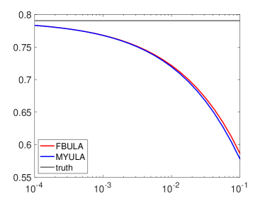
(a) $\mathbb{E}(x_{1})$

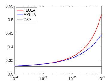
(b) $\text{Var}(x_{1})$

Figure 1: This figure compares the MY and FB envelopes for the two-dimensional truncated Gaussian distribution $\mathfrak{p}\propto e^{-U-1_{K_{2}}}$ specified in Section 7.1. The horizontal lines in the left and right panels show, respectively, the expectation and variance of the first coordinate, namely, $\mathbb{E}_{\mathfrak{p}}[x_{1}]$ and $\mathrm{var}_{\mathfrak{p}}[x_{1}]=\mathbb{E}_{\mathfrak{p}}[x_{1}^{2}]-(\mathbb{E}_{\mathfrak{p}}[x_{1}])^{2}$. The blue and red graphs in both panels show the estimated values of $\mathbb{E}_{\mathfrak{p}}[x_{1}]$ and $\mathrm{var}_{\mathfrak{p}}[x_{1}]$, obtained via MY and FB envelopes. That is, the graphs on the left correspond to $\mathbb{E}_{\mathfrak{p}_{\gamma}^{\textup{MY}}}[x_{1}]$ and $\mathbb{E}_{\mathfrak{p}_{\gamma}^{\textup{FB}}}[x_{1}]$, for various values of $\gamma$. Similarly, the graphs on the right correspond to $\mathrm{var}_{\mathfrak{p}_{\gamma}^{\textup{MY}}}[x_{1}]$ and $\mathrm{var}_{\mathfrak{p}_{\gamma}^{\textup{FB}}}[x_{1}]$, for various values of $\gamma$.

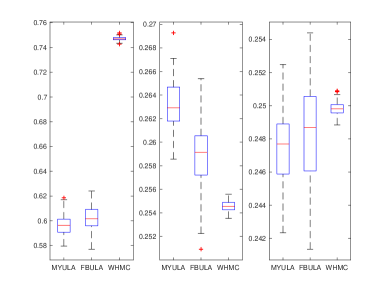
Figure 2: This figure shows the boxplots for the expectations of $x_{1},x_{2},x_{3}$ for the truncated Gaussian distribution in dimension $10$ obtained by MYULA, FBULA, and wHMC. The last approach serves as the ground truth.

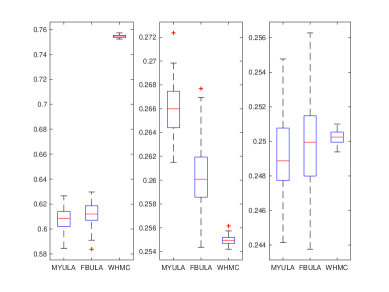
Figure 3: Boxplots for the expectations of $x_{1},x_{2},x_{3}$ for the truncated Gaussian distribution in dimension $100$, obtained by MYULA, FBULA, and wHMC. The last approach serves as the ground truth.

Such explicit calculations are not tractable in higher dimensions, i.e., for $d\in\{10,100\}$. Instead, we now generate $10^{6}$ samples from the truncated Gaussian distribution $\mathfrak{p}$ by applying MYULA and FBULA. As our ground truth, we also generate $10^{5}$ samples from $\mathfrak{p}$ with the wall HMC (wHMC) [26]. In all three approaches, the initial $10\%$ of the obtained samples are discarded as the burn-in period. In terms of the parameters, we set $\gamma=0.05$ and fix $h=0.005$ for all of our experiments.

The results are visualized in Figures 2 and 3. More specifically, Figure 2 corresponds to $d=10$ and shows the estimates for $\mathbb{E}_{\mathfrak{p}}[x_{i}]$ for $i\in\{1,2,3\}$, obtained by MYULA, FBULA, and wHMC. Similarly, Figure 3 corresponds to $d=100$. These figures indicate that, in all of these cases, FBULA is providing a more accurate approximation of the expectation compared to MYULA.

7.2 Tomographic image reconstruction

We now study a tomographic image reconstruction problem. In this case the true image is taken to the Shepp-Logan phantom test image of dimension $d=128\times 128$, in which we applied a Fourier operator $F$ followed by a subsampling operator $A$, reducing the observed pixels by approximately $85\%$. Finally, zero-mean additive Gaussian noise $\xi$ is added with standard deviation $\sigma=10^{-2}$ to produce an incomplete observation $y=AFx+\xi$ where $y\in\mathbb{C}^{p}$. Note that $p<d$. With regards to the prior, we use the total-variation norm with an additional constraint for the size of the pixels. This leads to the following posterior distribution:

$$\pi(x)\propto\exp\left[-\|y-AFx\|^{2}/2\sigma^{2}-\beta\text{TV}(x)-1_{\left[0,1\right]^{d}}(x)\right],$$ (33)

with $\beta=100$. Above, $1_{[0,1]^{d}}$ is the convex indicator function on the unit cube, as the pixel values for this experiment are scaled to the range $[0,1]$. Following (4) and (6b), we have that $f(x)=\|y-AFx\|^{2}/2\sigma^{2}$ and $g(x)={\beta}\text{TV}(x)+1_{\left[0,1\right]^{d}}(x)$. Figure 4(a) shows the Shepp-Logan phantom tomography test image for this experiment and Figure 4(b) shows the amplitude of the (noisy) Fourier coefficients collected in the observation vector $y$ (in logarithmic scale). In this figure, black regions represent unobserved pixels.

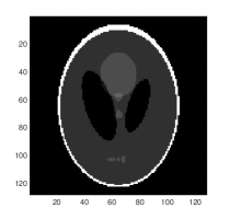
(a) True image $x$

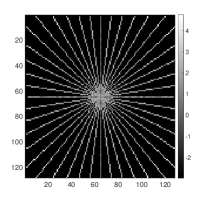
(b) Observation $y$

Figure 4: Tomography experiment: (a) True image $x$ of dimension $d=128\times 128$. (b) Incomplete and noisy observation $y$, amplitude of Fourier coefficients in logarithmic scale.

We have set $\gamma=1/5L_{f}$ where $L_{f}=1/\sigma^{2}=10^{4}$ for both MYULA and FBULA. Figure 5(a) shows the evolution of the values of $\log\pi(x)$ from (33) of both MYULA and FBULA with the step-size $h=1/(L_{f}+1/\gamma)=1.67\times 10^{-5}$. We observe that both methods converge at a similar rate. However, Figure 5(b) shows the evolution of the mean-squared error (MSE) between the ergodic mean of the samples and the true image $x$. Here, it can be seen FBULA reaches a better MSE level compared to MYULA. We have also included in Figure 5(c),(d) the posterior mean estimated by both MYULA and FBULA.

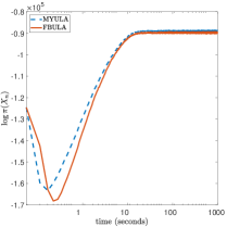
(a) $\log\pi^{\gamma}(x)$

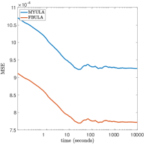
(b) MSE

(c) MYULA: posterior mean.

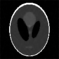
(d) FBULA: posterior mean.

Figure 5: Tomography experiment: (a) Convergence to the typical set of the posterior distribution (33). (b) Evolution of the MSE in stationarity. Posterior mean of (33) as estimated with (c) MYULA and (d) FBULA, respectively, after $10^{6}$ iterations.

Appendix A Proof of Proposition 3.1

To establish the admissibility of the MY envelopes, we verify the conditions in Definition 2.2. We begin by verifying that Definition 2.2(iii) is met. Recall that the MY envelope is continuously-differentiable [27, Theorem 2.26], and its gradient is given by

$$\nabla F_{\gamma}^{\textup{MY}}(x)=\nabla f(x)+\frac{x-P_{\gamma g}(x)}{\gamma},\qquad x\in\mathbb{R}^{d},$$ (A.1)

where

$$P_{\gamma g}:x\rightarrow\operatorname*{arg\,min}_{z\in\mathbb{R}^{d}}\left\{g(z)+\frac{1}{2\gamma}\|x-z\|_{2}^{2}\right\}$$ (A.2)

is the proximal operator associated with the function $\gamma g$. Above, note that the minimizer is unique and the map $P_{\gamma g}$ is thus well-defined. Recall also that we can use the Moreau decomposition [28] to write that

$$x=P_{\gamma g}(x)+P_{\gamma g^{*}(\cdot/\gamma)}(x),\qquad x\in\mathbb{R}^{d},$$ (A.3)

where $g^{*}$ is the Fenchel conjugate of $g$. Using (A.3), we rewrite (A.1) as

$$\nabla F^{\textup{MY}}_{\gamma}(x)=\nabla f(x)+\frac{P_{\gamma g^{*}(\cdot/\gamma)}(x)}{\gamma},$$ (A.4)

which we will use next to compute the Lipschitz constant of $\nabla F_{\gamma}^{\textup{MY}}$. For $x,y\in\mathbb{R}^{d}$, note that

$$\|\nabla F_{\gamma}^{\textup{MY}}(x)-\nabla F_{\gamma}^{\textup{MY}}(y)\|_{2}$$

$$\leq\|\nabla f(x)-\nabla f(y)\|_{2}+\frac{1}{\gamma}\|P_{\gamma g^{*}(\cdot/\gamma)}(x)-P_{\gamma g^{*}(\cdot/\gamma)}(y)\|_{2}\qquad\text{(see \eqref{eq:eqGrad})}$$

$$\leq\lambda_{2}+\frac{1}{\gamma},\qquad\text{(\eqref{eq:gradLipschitz} and non-expansiveness of the proximal operator)}$$ (A.5)

where the first line above uses the triangle inequality. We next verify that Definition 2.2(ii) holds. In one direction, it is easy to see that $g_{\gamma}\leq g$ for every $\gamma>0$. In the other direction, we fix $x\in\mathbb{R}^{d}$ and distinguish two cases:

1. When $x\in\mathrm{K}$, let us fix an arbitrary $\epsilon>0$. Because $g(x)<\infty$ and $\min_{z}g(z)>-\infty$ by (5), there exists a sufficiently small $\gamma_{\epsilon}>0$ such that the following holds for every $\gamma\leq\gamma_{\epsilon}$:

   $$\min_{z\in\mathbb{R}^{d}}\left\{g(z)+\frac{\epsilon^{2}}{2\gamma}\right\}>g(x).\qquad x\in\mathrm{K}.$$ (A.6)

   We now use the above inequality as part of the following argument,

   $$\min_{z\in\mathbb{R}^{d}}\left\{g(z)+\frac{1}{2\gamma}\|x-z\|_{2}^{2}:\|x-z\|\geq\epsilon\right\}$$

   $$\geq\min_{z}\left\{g(z)+\frac{\epsilon^{2}}{2\gamma}\right\}$$

   $$>g(x)\qquad\text{(see \eqref{eq:suffSmallGamma})}$$

   $$\geq g_{\gamma}(x)=\min_{z}\left\{g(z)+\frac{1}{2\gamma}\|x-z\|_{2}^{2}\right\},$$ (A.7)

   which holds when $x\in\mathrm{K}$ and for every $\gamma\leq\gamma_{\epsilon}$. In view of (A.2) and (A.7), we conclude that $\|x-P_{\gamma g}(x)\|_{2}\leq\epsilon$, for every $x\in\mathrm{K}$ and every $\gamma\leq\gamma_{\epsilon}$. Since the choice of $\epsilon$ was arbitrary, we arrive at

   $$\lim_{\gamma\rightarrow 0}\|x-P_{\gamma g}(x)\|_{2}=0,\qquad x\in\mathrm{K}.$$ (A.8)

   It immediately follows that

   $$\liminf_{\gamma\rightarrow 0}g_{\gamma}(x)-g(x)$$

   $$=\liminf_{\gamma\rightarrow 0}\min_{z}\left\{g(z)+\frac{1}{2\gamma}\|x-z\|_{2}^{2}\right\}-g(x)\qquad\text{(see \eqref{eq:MYEnv})}$$

   $$=\liminf_{\gamma\rightarrow 0}\left\{g(P_{\gamma g}(x))+\frac{1}{2\gamma}\|x-P_{\gamma g}(x)\|_{2}^{2}\right\}-g(x)\qquad\text{(see \eqref{eq:proxDefn})}$$

   $$\geq\liminf_{\gamma\rightarrow 0}g(P_{\gamma g}(x))-g(x)$$

   $$\geq\liminf_{z\rightarrow x}g(z)-g(x)\qquad\text{(see \eqref{eq:insideC})}$$

   $$\geq 0,\qquad x\in\mathrm{K},$$ (A.9)

   where the last inequality follows from the fact that $g$ is lower semi-continuous, see above Equation (5). If we combine (A.9) with the earlier observation that $g_{\gamma}\leq g$ for every $\gamma$, we reach the conclusion that $\lim_{\gamma\rightarrow 0}g_{\gamma}(x)=g(x)$, provided that $x\in\mathrm{K}$. Lastly, after recalling the definitions of $F$ and $F_{\gamma}^{\textup{MY}}$ in (6b) and (MY), respectively, we arrive at

   $$\lim_{\gamma\rightarrow 0}F^{\textup{MY}}_{\gamma}(x)=F(x),\qquad x\in\mathrm{K}.$$ (A.10)

2. When $x\notin\mathrm{K}$, note that $g(x)=\infty$ by (5). Note also that

   $$g_{\gamma}(x) =\min_{z}\left\{g(z)+\frac{1}{2\gamma}\|x-z\|_{2}^{2}\right\}\qquad\text{(see \eqref{eq:MY})}$$

   $$=\min\left\{g(z)+\frac{1}{2\gamma}\|x-z\|^{2}_{2}:z\in\mathrm{K}\right\}\qquad\text{(see \eqref{eq:propsG})}$$

   $$\geq-\max_{z\in\mathrm{K}}g(z)+\frac{1}{2\gamma}\min_{z\in\mathrm{K}}\|x-z\|_{2}^{2}$$

   $$=:-\max_{z\in\mathrm{K}}g(z)+\frac{1}{2\gamma}\operatorname{dist}(x,\mathrm{K})^{2},$$ (A.11)

   where $\operatorname{dist}(x,\mathrm{K})$ is the Euclidean distance from $x$ to the set $\mathrm{K}$. The maximum above is finite by (5). Above, by sending $\gamma$ to zero, we immediately find that $\lim_{\gamma\rightarrow 0}g_{\gamma}(x)=\infty=g(x)$, provided that $x\notin\mathrm{K}$. Recalling the definition of $F$ and $F_{\gamma}$ in (6b) and (MY), we conclude that

   $$\lim_{\gamma\rightarrow 0}F_{\gamma}^{\textup{MY}}(x)=F(x)=\infty,\qquad x\notin\mathrm{K}.$$ (A.12)

Together, (A.8) and (A.12) imply that $\lim_{\gamma\rightarrow 0}F_{\gamma}(x)=F(x)$ for every $x\in\mathbb{R}^{d}$.

Lastly, we now verify that Definition 2.2(i) is satisfied: Because, by Assumption 2.2(i), $\mathrm{K}$ is enclosed inside a ball of radius $R$ centered at the origin, it holds that

$$\operatorname{dist}(x,\mathrm{K})\geq(\|x\|-R)_{+},\qquad x\in\mathbb{R}^{d},$$ (A.13)

where $(a)_{+}:=\max(a,0)$. When $\|x\|_{2}$ is sufficiently large, we can simplify (A.13). In particular, (A.13) immediately implies that

$$\operatorname{dist}(x,\mathrm{K})\geq\|x\|_{2}/2,\qquad\|x\|_{2}\geq 2R.$$ (A.14)

If $\|x\|_{2}\geq 2R$, then we can use the convexity of $f$ by Assumption 2.1(ii), in order to write that

$$F_{\gamma}^{\textup{MY}}(x) =f(x)+g_{\gamma}(x)\qquad\text{(see \eqref{eq:MYEnv})}$$

$$\geq f(0)+\langle x,\nabla f(0)\rangle+g_{\gamma}(x)\qquad(\text{convexity of }f)$$

$$\geq f(0)+\langle x,\nabla f(0)\rangle-\max_{z\in\mathrm{K}}g(z)+\frac{1}{2\gamma}\operatorname{dist}(x,\mathrm{K})^{2}\qquad\text{(see \eqref{eq:gToDist})}$$

$$\geq f(0)+\langle x,\nabla f(0)\rangle-\max_{z\in\mathrm{K}}g(z)+\frac{\|x\|_{2}^{2}}{8\gamma},\qquad\text{(see \eqref{eq:gToDist2})}$$ (A.15)

for $\|x\|_{2}\geq 2R$. We now set

$$F^{0}(x):=\begin{cases}F_{\gamma}(x)&\|x\|_{2}\leq 2R\\ f(0)+\langle x,\nabla f(0)\rangle-\max_{z\in\mathrm{K}}g(z)+\frac{\|x\|_{2}^{2}}{8\gamma}&\|x\|_{2}\geq 2R.\end{cases}$$ (A.16)

By its construction, note that $F^{0}$ satisfies $\int e^{-F^{0}(x)}\,\operatorname{d}x<\infty$ and $F^{0}\geq F_{\gamma}$, as required in Definition 2.2(i). The former claim is true because $F^{0}(x)$ is quadratic for large $\|x\|_{2}$ and $e^{-F^{0}}$ thus decays rapidly faraway from the origin. This completes the proof of Proposition 3.1.

Appendix B Proof of Proposition 4.2

To establish the admissibility of the FB envelopes, we verify the requirements in Definition 2.2. We first verify that Definition 2.2(iii) holds. To begin, for $x\in\mathbb{R}^{d}$, let

$$\overline{x}:=x-\gamma\nabla f(x),\qquad T_{\gamma}(x):=P_{\gamma g}(\overline{x}),$$ (B.17)

for short. Above, recall that $P_{\gamma g}$ is the proximal operator associated with the function $\gamma g$, see (9). We can then apply the Moreau decomposition [28] to write that

$$\overline{x}=P_{\gamma g}(\overline{x})+P_{\gamma g^{*}(\cdot/\gamma)}(\overline{x}),$$ (B.18)

where $g^{*}$ is the Fenchel conjugate of $g$. For future reference, we record the following observations:

$$\|T_{\gamma}(x)\|_{2} =\|P_{\gamma g}(\overline{x})\|_{2}\leq R,\qquad\text{(combine Assumption~{}\ref{assumption:fg}\ref{item:CAssumption} and \eqref{eq:gToDist})}$$ (B.19)

$$\|x-T_{\gamma}(x)\|_{2} \leq\|x\|_{2}+\|T_{\gamma}(x)\|_{2}\leq\|x\|_{2}+R,\qquad\text{(see \eqref{eq:normTx})}$$ (B.20)

$$\|x-y-(T_{\gamma}(x)-T_{\gamma}(y))\|_{2}$$

$$=\|x-y-(P_{\gamma g}(\overline{x})-P_{\gamma g}(\overline{y}))\|_{2}\qquad\text{(see \eqref{eq:shortHands})}$$

$$=\|\gamma(\nabla f(x)-\nabla f(y))+(P_{\gamma g^{*}(\cdot/\gamma)}(\overline{x})-P_{\gamma g^{*}(\cdot/\gamma)}(\overline{x}))\|_{2}\quad\text{(see \eqref{eq:2ndMeuro})}$$

$$\leq\gamma\|\nabla f(x)-\nabla f(y)\|_{2}+\left\|P_{\gamma g^{*}(\cdot/\gamma)}(\overline{x})-P_{\gamma g^{*}(\cdot/\gamma)}(\overline{x})\right\|_{2}$$

$$\leq\gamma\lambda_{2}\|x-y\|+\|\overline{x}-\overline{y}\|_{2}\qquad(\text{\eqref{eq:gradLipschitz} and non-expansiveness of }P_{\gamma g^{*}(\cdot/\gamma)})$$

$$\leq\gamma\lambda_{2}\|x-y\|_{2}+\|x-y\|_{2}+\gamma\|\nabla f(x)-\nabla f(y)\|_{2}\qquad\text{(see \eqref{eq:shortHands})}$$

$$\leq(1+2\gamma\lambda_{2})\|x-y\|,\qquad\text{(see \eqref{eq:gradLipschitz})}$$ (B.21)

$$0\prec(1-\gamma\lambda_{2})I_{d}\preccurlyeq I_{d}-\gamma\nabla^{2}f(x)\preccurlyeq I_{d},$$

$$\|I_{d}-\gamma\nabla^{2}f(x)\|\leq 1.\qquad(\text{\eqref{eq:gradLipschitz} and }\gamma\in(0,1/\lambda_{2}))$$ (B.22)

Above, $I_{d}\in\mathbb{R}^{d\times d}$ is the identity matrix. Recall the expression for $\nabla F_{\gamma}^{\textup{FB}}$ from Proposition 4.1(iii). We next establish that $F_{\gamma}^{\textup{FB}}$ is smooth. Below, without loss of generality, we can assume that $\|y\|_{2}\leq\lambda_{0}$:

$$\|\nabla F^{\textup{FB}}_{\gamma}(x)-\nabla F^{\textup{FB}}_{\gamma}(x)\|_{2}$$

$$=\frac{1}{\gamma}\|(I_{d}-\gamma\nabla^{2}f(x))(x-T_{\gamma}(x))-(I_{d}-\gamma\nabla^{2}f(y))(y-T_{\gamma}(y))\|_{2}\qquad\text{(Proposition~{}\ref{prop:propsFB}\ref{item:derFB})}$$

$$\leq\frac{1}{\gamma}\left\|(I_{d}-\gamma\nabla^{2}f(x))(x-y-(T_{\gamma}(x)-T_{\gamma}(y))\right\|_{2}+\left\|(\nabla^{2}f(x)-\nabla^{2}f(y))(y-T_{\gamma}(y))\right\|_{2}$$

$$\leq\frac{1+2\gamma\lambda_{2}}{\gamma}\|x-y\|_{2}+\lambda_{3}(\|y\|_{2}+R)\|x-y\|_{2}\qquad\text{(see \eqref{eq:hessianLipschitz} and \eqref{eq:x-Tx}-\eqref{eq:specofR})}$$

$$\leq\frac{1+2\gamma\lambda_{2}}{\gamma}\|x-y\|_{2}+\lambda_{3}(\lambda_{0}+R)\|x-y\|_{2}\qquad(\|y\|_{2}\leq\lambda_{0}\text{ without loss of generality})$$

$$=(\gamma^{-1}+2\lambda_{2}+\lambda_{3}(\lambda_{0}+R))\|x-y\|_{2}$$

$$=:\lambda_{\gamma}^{\textup{FB}}\|x-y\|_{2}.$$ (B.23)

Indeed, if both $\|x\|_{2}\geq\lambda_{0}$ and $\|y\|_{2}\geq\lambda_{0}$, then $f(x)=f(y)=\|\nabla f(x)\|_{2}=\|\nabla f(y)\|_{2}=\|\nabla^{2}f(x)\|=\|\nabla^{2}f(y)\|=0$ by (3), and (B.23) still holds. This observation justfies our earlier restriction to the case where $\|y\|_{2}\leq\lambda_{0}$. Next, we show the strong convexity of $F_{\gamma}^{\textup{FB}}$ over long distances. Again, without loss of generality, we assume below that $\|y\|_{2}\leq\lambda_{0}$ and write that

$$\langle x-y,\nabla F_{\gamma}^{\textup{FB}}(x)-\nabla F_{\gamma}^{\textup{FB}}(y)\rangle$$

$$=\frac{1}{\gamma}\left\langle x-y,(I_{d}-\gamma\nabla^{2}f(x))(x-T_{\gamma}(x))-(I_{d}-\gamma\nabla^{2}f(y))(y-T_{\gamma}(y))\right\rangle$$

$$=\frac{1}{\gamma}\left\langle x-y,(I_{d}-\gamma\nabla^{2}f(x))(x-y-(T_{\gamma}(x)-T_{\gamma}(y)))\right\rangle$$

$$\qquad-\left\langle x-y,(\nabla^{2}f(x)-\nabla^{2}f(y))(y-T_{\gamma}(y))\right\rangle$$

$$\geq\frac{1}{\gamma}\langle x-y,(I_{d}-\gamma\nabla^{2}f(x))(x-y)\rangle-\frac{\|I_{d}-\gamma\nabla^{2}f(x)\|}{\gamma}\|x-y\|_{2}(\|T_{\gamma}(x)\|_{2}+\|T_{\gamma}(y)\|_{2})$$

$$\qquad-\|x-y\|_{2}\cdot\|\nabla^{2}f(x)-\nabla^{2}f(y)\|\cdot\|y-T_{\gamma}(y)\|_{2}$$

$$\geq\frac{1-\gamma\lambda_{2}}{\gamma}\|x-y\|_{2}^{2}$$

$$\qquad-\frac{2R}{\gamma}\|x-y\|_{2}-\lambda_{3}(\lambda_{0}+R)\|x-y\|_{2}^{2}\qquad\text{(see \eqref{eq:hessianLipschitz}, \eqref{eq:normTx}, \eqref{eq:x-Tx}, \eqref{eq:specofR})}$$

$$=\frac{1}{\gamma}(1-\gamma(\lambda_{2}+\lambda_{3}(\lambda_{0}+R)))\|x-y\|_{2}^{2}-\frac{2R}{\gamma}\|x-y\|_{2},$$ (B.24)

where the second line uses Proposition 4.1(iii). When $\|x-y\|_{2}$ is sufficiently large, the first term in the last line above dominates the second term. In particular, it holds that

$$\|x-y\|_{2}\geq\rho_{\gamma}^{\textup{FB}}:=\frac{2R}{1-2\gamma(\lambda_{2}+\lambda_{3}(\lambda_{0}+R)))}$$

$$\qquad\Longrightarrow\langle x-y,\nabla F_{\gamma}^{\textup{FB}}(x)-\nabla F_{\gamma}^{\textup{FB}}(y)\rangle\geq(\lambda_{2}+\lambda_{3}(\lambda_{0}+R))\|x-y\|_{2}^{2}.$$ (B.25)

In words, $F^{\textup{FB}}_{\gamma}$ behaves like a strongly convex function over long distances. It is not difficult to verify that Definition 2.2(ii) is also valid for the FB envelopes: To that end, one needs to combine Proposition 3.1 with the relation between the MY and FB envelopes in Proposition 4.1(ii).

Lastly, we now verify that the requirement in Definition 2.2(i) is met for the FB envelopes: Below, suppose that $\gamma\in(0,1/\lambda_{2})$. On the one hand, Proposition 4.1(ii) implies that

$$F^{\textup{FB}}_{\gamma}\geq F^{\textup{MY}}_{\frac{\gamma}{1-\gamma\lambda_{2}}}.$$

On the other hand, by Proposition 3.1, there exists $F^{0}\leq F_{\frac{\gamma}{1-\gamma\lambda_{2}}}^{\textup{MY}}$ such that $e^{-F^{0}}$ is integrable. By combining the preceding two observations, we find that the FB envelopes satisfy Definition 2.2(i) for every $\gamma\in(0,1/\lambda_{2})$. This completes the proof of Proposition 4.2.

Appendix C Proof of Theorem 4.4

Let us define

$$\mathfrak{q}(x):=\frac{e^{f(x)-1_{\mathrm{K}}(x)}}{\int_{z}e^{f(z)-1_{\mathrm{K}}(z)}\,\operatorname{d}z},\qquad x\in\mathbb{R}^{d},$$ (C.26)

where $1_{\mathrm{K}}$ is the indicator function on the set $\mathrm{K}$. Note that the target distribution $\mathfrak{p}$ in (6a) coincides with $\mathfrak{q}$ in the special case where $g=1_{\mathrm{K}}$. Let $\operatorname{dist}(x,\mathrm{K})$ denote the distance from $x$ to the set $\mathrm{K}$. For $\gamma>0$, we also define

$$1_{\mathrm{K},\gamma}(x):=\frac{1}{2\gamma}\operatorname{dist}(x,\mathrm{K})^{2}=\frac{1}{2\gamma}\min_{z\in\mathrm{K}}\|x-z\|_{2}^{2}$$

$$=\min_{z\in\mathbb{R}^{d}}\left\{1_{\mathrm{K}}(x)+\frac{1}{2\gamma}\|x-z\|_{2}^{2}\right\},\qquad x\in\mathbb{R}^{d},$$ (C.27)

to be the MY envelope of the indicator function on the set $\mathrm{K}$. We denote the corresponding probability distribution by

$$\mathfrak{q}_{\gamma}(x):=\frac{e^{f(x)-1_{\mathrm{K},\gamma}(x)}}{\int_{z}e^{f(z)-1_{\mathrm{K},\gamma}(z)}\,\operatorname{d}z},\qquad x\in\mathbb{R}^{d}.$$ (C.28)

When $\gamma$ is sufficiently small, we may intuitively regard $\mathfrak{q}_{\gamma}$ as a proxy for $\mathfrak{q}$. We also recall our earlier notation for the convenience of the reader:

$$\mathfrak{p}(x)=\frac{e^{-F(x)}}{\int_{z}e^{-F(z)}\,\operatorname{d}z},\qquad\mathfrak{p}^{\textup{FB}}_{\gamma}(x)=\frac{e^{-F^{\textup{FB}}_{\gamma}(x)}}{\int_{z}e^{-F^{\textup{FB}}_{\gamma}(z)}\,\operatorname{d}z},\qquad x\in\mathbb{R}^{d}.$$ (C.29)

Above, the functions $F$ and $F^{\textup{FB}}_{\gamma}$ were defined in (6b) and (FB), respectively. Our objective is to control the distance $\mathrm{W}_{1}(\mathfrak{p}^{\textup{FB}}_{\gamma},\mathfrak{p})$. To begin, we use the triangle inequality to write that

$$\mathrm{W}_{1}(\mathfrak{p}^{\textup{FB}}_{\gamma},\mathfrak{p})\leq\mathrm{W}_{1}(\mathfrak{p}^{\textup{FB}}_{\gamma},\mathfrak{q}_{\gamma})+\mathrm{W}_{1}(\mathfrak{q}_{\gamma},\mathfrak{q})+\mathrm{W}_{1}(\mathfrak{q},\mathfrak{p}).$$ (C.30)

The following three lemmas each bounds one of the terms on the right-hand side above.

Lemma C.1.

It holds that

$$\mathrm{W}_{1}(\mathfrak{p}^{\textup{FB}}_{\gamma},\mathfrak{q}_{\gamma})\leq\Cr{dist1}+\Cr{dist2}\frac{I_{2}(\gamma/(1-\gamma\lambda_{2})))}{\textup{vol}(\mathrm{K})+I_{1}(\gamma)},$$ (C.31)

where

$$\Cr{dist1}:=\frac{e^{2\max_{x\in\mathrm{K}}g(x)-\gamma\lambda_{2}\min_{z}f(z)}\int_{\mathrm{K}}\|x\|_{2}e^{-(1-\gamma\lambda_{2})f(x)}\,\operatorname{d}x}{\int e^{-f(x)-\frac{\operatorname{dist}(x,\mathrm{K})^{2}}{2\gamma}}\,\operatorname{d}x}$$

$$\qquad-\frac{e^{\gamma\lambda_{2}\min_{z}f(z)-2\max_{x\in\mathrm{K}}g(x)}\int_{\mathrm{K}}\|x\|_{2}e^{-f(x)}\,\operatorname{d}x}{\int e^{-(1-\gamma\lambda_{2})f(x)-\frac{\operatorname{dist}(x,\mathrm{K})^{2}}{2\gamma/(1-\gamma\lambda_{2})}}\,\operatorname{d}x},$$

$$\Cr{dist2}:=e^{\max_{x}f(x)-\min_{x}f(x)+2\max_{x\in\mathrm{K}}g(x)},$$

$$I_{1}(\gamma):=\sum_{i=0}^{d-1}\textup{vol}_{i}(\mathrm{K})\cdot(2\pi\gamma)^{\frac{d-i}{2}},$$

$$I_{2}(\gamma):=\sum_{i=0}^{d-1}\textup{vol}_{i}(\mathrm{K})\cdot(2\pi\gamma)^{\frac{d-i}{2}}\left(\sqrt{\gamma(d-i+3)}+R\right)=:I_{2}(\gamma),$$ (C.32)

where $\textup{vol}_{i}(\mathrm{K})$ is the $i$-th intrinsic volume of $\mathrm{K}$ [25]. In particular, the $d$-th volume of $\mathrm{K}$ coincides with the standard volume of $\mathrm{K}$, i.e., $\textup{vol}_{d}(\mathrm{K})=\textup{vol}(\mathrm{K})$.

Lemma C.2.

It holds that

$$\mathrm{W}_{1}(\mathfrak{q}_{\gamma},\mathfrak{q})\leq\Cr{dist3}\frac{RI_{1}(\gamma)+I_{2}(\gamma)}{\textup{vol}(\mathrm{K})+I_{1}(\gamma)},$$ (C.33)

where $\Cr{dist3}:=e^{\max_{x}f(x)-\min_{x}f(x)}$.

Lemma C.3.

It holds that

$$\mathrm{W}_{1}(\mathfrak{q},\mathfrak{p})\leq\Cr{dist4}R,$$ (C.34)

where

$$\Cr{dist4}:=e^{\max_{x\in\mathrm{K}}g(x)-\min_{x\in\mathrm{K}}g(x)}-e^{\min_{x\in\mathrm{K}}g(x)-\max_{x\in\mathrm{K}}g(x)}.$$ (C.35)

To keep the notation light, above we have suppressed the dependence of $\Cr{dist1}$ to $\Cr{dist4}$ on $\mathrm{K},f,g$. With Lemmas C.1-C.3 at hand, we revisit (C.30) and write that

$$\mathrm{W}_{1}(\mathfrak{p}_{\gamma}^{\textup{FB}},\mathfrak{p})\leq\Cr{dist1}+\frac{\Cr{dist3}RI_{1}(\gamma)+\Cr{dist3}I_{2}(\gamma)+\Cr{dist2}I_{2}(\gamma/(1-\gamma\lambda_{2}))}{\textup{vol}(\mathrm{K})+I_{1}(\gamma)}+\Cr{dist4}R.$$ (C.36)

This completes the proof of Proposition 4.4.

Appendix D Proof of Lemma C.1

In order to upper bound the distance $\mathrm{W}_{1}(\mathfrak{q}_{\gamma},\mathfrak{p}_{\gamma}^{\textup{FB}})$, we will use the following simple result which bounds the $\mathrm{W}_{1}$ distance under small perturbations.

Lemma D.1.

For constants $\alpha\geq\beta$ and $\beta^{\prime}\leq 1$, consider two functions $h_{1}:\mathbb{R}^{d}\rightarrow\mathbb{R}$ and $h_{2}:\mathbb{R}^{d}\rightarrow\mathbb{R}$ that are related as

$$\beta^{\prime}\cdot h_{1}(x)+\beta\leq h_{2}(x)\leq h_{1}(x)+\alpha,\qquad x\in\mathbb{R}^{d},$$ (D.37)

Then it holds that

$$\mathrm{W}_{1}\left(\frac{e^{-h_{1}}}{\int e^{-h_{1}}},\frac{e^{-h_{2}}}{\int e^{-h_{2}}}\right)$$

$$\leq\frac{e^{\alpha-\beta}\int\|x\|_{2}e^{-\beta^{\prime}h_{1}(x)}\,\operatorname{d}x}{\int e^{-h_{1}(x)}\,\operatorname{d}x}-\frac{e^{\beta-\alpha}\int\|x\|_{2}e^{-h_{1}(x)}\,\operatorname{d}x}{\int e^{-\beta^{\prime}h_{1}(x)}\,\operatorname{d}x}.$$ (D.38)

As a sanity check, note that the right-hand side of (D.38) is always nonnegative because, by assumption, $\alpha\geq\beta$ and $\beta^{\prime}\leq 1$. Moreover, if we set $\alpha=\beta=0$ and $\beta^{\prime}=1$, the right-hand side of (D.38) reduces to zero, as expected.

Let us now recall from (C.28) and (6a) that $\mathfrak{q}_{\gamma}\propto e^{-f-1_{\mathrm{K},\gamma}}$ and $\mathfrak{p}_{\gamma}^{\textup{FB}}\propto e^{-F^{\textup{FB}}_{\gamma}}$, respectively. Our plan is to invoke Lemma D.1 with the choice of $h_{1}=f+1_{\mathrm{K},\gamma}$ and $h_{2}=F^{\textup{FB}}_{\gamma}$. In turn, this plan necessitates that we verify (D.37) for the choice of $h_{1}=f+1_{\mathrm{K},\gamma}$ and $h_{2}=F^{\textup{FB}}_{\gamma}$. We begin by relating the two functions as

$$F^{\textup{FB}}_{\gamma}(x) \leq F^{\textup{MY}}_{\gamma}(x)\qquad\text{(Proposition \ref{prop:propsFB}\ref{item:sandwitch2})}$$

$$=f(x)+g_{\gamma}(x)\qquad\text{(see \eqref{eq:MYEnv})}$$

$$=f(x)+\min_{z\in\mathrm{K}}\left\{g(z)+\frac{1}{2\gamma}\|x-z\|_{2}^{2}\right\}\qquad\text{(see \eqref{eq:MY})}$$

$$\leq\max_{z\in\mathrm{K}}g(z)+f(x)+\frac{1}{2\gamma}\min_{z\in\mathrm{K}}\|x-z\|_{2}^{2}$$

$$=\max_{z\in\mathrm{K}}g(z)+f(x)+1_{\mathrm{K},\gamma}(x)\qquad\text{(see \eqref{eq:MYenvOfInd})}.$$ (D.39)

Above, note that $\max_{z\in\mathrm{K}}g(z)$ is finite by the construction of $g$, see (5). In the other direction, we similarly write that

$$F^{\textup{FB}}_{\gamma}(x)$$

$$\geq F^{\textup{MY}}_{\frac{\gamma}{1-\gamma\lambda_{2}}}(x)\qquad\text{(Proposition \ref{prop:propsFB}\ref{item:sandwitch2})}$$

$$=f(x)+g_{\frac{\gamma}{1-\gamma\lambda_{2}}}(x)$$

$$=f(x)+\min_{z}\left\{g(z)+\frac{1-\gamma\lambda_{2}}{2\gamma}\|x-z\|_{2}^{2}\right\}$$

$$\geq-\max_{z\in\mathrm{K}}g(z)+f(x)+\frac{1-\gamma\lambda_{2}}{2\gamma}\min_{z\in\mathrm{K}}\|x-z\|_{2}^{2}$$

$$=-\max_{z\in\mathrm{K}}g(z)+\gamma\lambda_{2}f(x)+(1-\gamma\lambda_{2})f(x)+(1-\gamma\lambda_{2})1_{\mathrm{K},\gamma}(x)\qquad\text{(see \eqref{eq:MYenvOfInd})}$$

$$\geq-\max_{z\in\mathrm{K}}g(z)+\gamma\lambda_{2}\min_{z}f(z)+(1-\gamma\lambda_{2})f(x)+(1-\gamma\lambda_{2})1_{\mathrm{K},\gamma}(x).$$ (D.40)

Above, $\min_{z}f(z)$ is finite by the construction of $f$, see (3). To summarize, for our choice of $h_{1}=f+1_{\mathrm{K},\gamma}$ and $h_{2}=F^{\textup{FB}}_{\gamma}$, (D.37) is satisfied with

$$\beta^{\prime}(f(x)+1_{\mathrm{K},\gamma}(x))+\beta\leq F^{\textup{FB}}_{\gamma}(x)\leq f(x)+1_{\mathrm{K},\gamma}(x)+\alpha,\qquad x\in\mathbb{R}^{d},$$ (D.41)

$$\alpha=\max_{z\in\mathrm{K}}g(z),\quad\beta=\gamma\lambda_{2}\min_{z}f(z)-\max_{z\in\mathrm{K}}g(z),\quad\beta^{\prime}=1-\gamma\lambda_{2}.$$

With (D.41) at hand, we can invoke Lemma D.1 to find that

$$\mathrm{W}_{1}(\mathfrak{q}_{\gamma},\mathfrak{p}_{\gamma}^{\textup{FB}}) =\mathrm{W}_{1}\left(\frac{e^{-f-1_{\mathrm{K},\gamma}}}{\int e^{-f-1_{\mathrm{K},\gamma}}},\frac{e^{-F_{\gamma}^{\textup{FB}}}}{\int e^{-F_{\gamma}^{\textup{FB}}}}\right)$$

$$\leq\frac{e^{\alpha-\beta}\int\|x\|_{2}e^{-\beta^{\prime}f(x)-\beta^{\prime}1_{\mathrm{K},\gamma}(x)}\,\operatorname{d}x}{\int e^{-f(x)-1_{\mathrm{K},\gamma}(x)}\,\operatorname{d}x}-\frac{e^{\beta-\alpha}\int\|x\|_{2}e^{-f(x)-1_{\mathrm{K},\gamma}(x)}\,\operatorname{d}x}{\int e^{-\beta^{\prime}f(x)-\beta^{\prime}1_{\mathrm{K},\gamma}(x)}\,\operatorname{d}x}$$

$$=\frac{e^{2\max_{x\in\mathrm{K}}g(x)-\gamma\lambda_{2}\min_{z}f(z)}\int\|x\|_{2}e^{-(1-\gamma\lambda_{2})f(x)-\frac{\operatorname{dist}(x,\mathrm{K})^{2}}{2\gamma/(1-\gamma\lambda_{2})}}\,\operatorname{d}x}{\int e^{-f(x)-\frac{\operatorname{dist}(x,\mathrm{K})^{2}}{2\gamma}}\,\operatorname{d}x}$$

$$-\frac{e^{\gamma\lambda_{2}\min_{z}f(z)-2\max_{x\in\mathrm{K}}g(x)}\int\|x\|_{2}e^{-f(x)-\frac{\operatorname{dist}(x,\mathrm{K})^{2}}{2\gamma}}\,\operatorname{d}x}{\int e^{-(1-\gamma\lambda_{2})f(x)-\frac{\operatorname{dist}(x,\mathrm{K})^{2}}{2\gamma/(1-\gamma\lambda_{2})}}\,\operatorname{d}x},$$ (D.42)

where the second line uses Lemma D.1 and the last line uses (C.27) and (D.41). To complete the proof, we need the following result, which is proved in [14, 29] using the well-known Steiner’s formula from integral geometry [25]. For completeness, a self-contained proof is given later.

Lemma D.2.

It holds that

$$\int_{\mathrm{K}^{c}}e^{-\frac{\operatorname{dist}(x,\mathrm{K})^{2}}{2\gamma}}\,\operatorname{d}x=\sum_{i=0}^{d-1}\textup{vol}_{i}(\mathrm{K})\cdot(2\pi\gamma)^{\frac{d-i}{2}}=:I_{1}(\gamma),$$ (D.43a)

$$\int_{\mathbb{R}^{d}}e^{-\frac{\operatorname{dist}(x,\mathrm{K})^{2}}{2\gamma}}\,\operatorname{d}x=\sum_{i=0}^{d}\textup{vol}_{i}(\mathrm{K})\cdot(2\pi\gamma)^{\frac{d-i}{2}}=\textup{vol}(\mathrm{K})+I_{1}(\gamma),$$ (D.43b)

$$\int_{\mathrm{K}^{c}}\|x\|_{2}e^{-\frac{\operatorname{dist}(x,\mathrm{K})^{2}}{2\gamma}}\,\operatorname{d}x$$

$$\leq\sum_{i=0}^{d-1}\textup{vol}_{i}(\mathrm{K})\cdot(2\pi\gamma)^{\frac{d-i}{2}}\left(\sqrt{\gamma(d-i+3)}+R\right)=:I_{2}(\gamma),$$ (D.43c)

where $\mathrm{K}^{c}=\mathbb{R}^{d}\backslash\mathrm{K}$ is the complement of the set $\mathrm{K}$ and $\textup{vol}_{i}(\mathrm{K})$ is the $i$-th intrinsic volume of $\mathrm{K}$ [25]. In particular, the $d$-th volume of $\mathrm{K}$ coincides with the standard volume of $\mathrm{K}$, i.e., $\textup{vol}_{d}(\mathrm{K})=\textup{vol}(\mathrm{K})$.

In particular, note that $I_{1}(\gamma)$ and $I_{2}(\gamma)$ both vanish in the limit of $\gamma\rightarrow 0$, as expected. To control the first fraction in the last line of (D.42), we use Lemma D.2 to write that

$$\frac{\int\|x\|_{2}e^{-(1-\gamma\lambda_{2})f(x)-\frac{\operatorname{dist}(x,\mathrm{K})^{2}}{2\gamma/(1-\gamma\lambda_{2})}}\,\operatorname{d}x}{\int e^{-f(x)-\frac{\operatorname{dist}(x,\mathrm{K})^{2}}{2\gamma}}\,\operatorname{d}x}$$

$$=\frac{\int_{\mathrm{K}}\|x\|_{2}e^{-(1-\gamma\lambda_{2})f(x)}\,\operatorname{d}x}{\int e^{-f(x)-\frac{\operatorname{dist}(x,\mathrm{K})^{2}}{2\gamma}}\,\operatorname{d}x}+\frac{\int_{\mathrm{K}^{c}}\|x\|_{2}e^{-(1-\gamma\lambda_{2})f(x)-\frac{\operatorname{dist}(x,\mathrm{K})^{2}}{2\gamma/(1-\gamma\lambda_{2})}}\,\operatorname{d}x}{\int e^{-f(x)-\frac{\operatorname{dist}(x,\mathrm{K})^{2}}{2\gamma}}\,\operatorname{d}x}$$

$$\leq\frac{\int_{\mathrm{K}}\|x\|_{2}e^{-(1-\gamma\lambda_{2})f(x)}\,\operatorname{d}x}{\int e^{-f(x)-\frac{\operatorname{dist}(x,\mathrm{K})^{2}}{2\gamma}}\,\operatorname{d}x}+\frac{e^{-(1-\gamma\lambda_{2})\min_{x}f(z)}}{e^{-\max_{x}f(z)}}\cdot\frac{I_{2}(\gamma/(1-\gamma\lambda_{2}))}{\textup{vol}(\mathrm{K})+I_{1}(\gamma)},$$ (D.44)

where the last line uses Lemma D.2. For the second fraction in the last line of (D.42), we similarly use Lemma D.2 to write that

$$\frac{\int\|x\|_{2}e^{-f(x)-\frac{\operatorname{dist}(x,\mathrm{K})^{2}}{2\gamma}}\,\operatorname{d}x}{\int e^{-(1-\gamma\lambda_{2})f(x)-\frac{\operatorname{dist}(x,\mathrm{K})^{2}}{2\gamma/(1-\gamma\lambda_{2})}}\,\operatorname{d}x}$$

$$=\frac{\int_{\mathrm{K}}\|x\|_{2}e^{-f(x)}\,\operatorname{d}x}{\int e^{-(1-\gamma\lambda_{2})f(x)-\frac{\operatorname{dist}(x,\mathrm{K})^{2}}{2\gamma/(1-\gamma\lambda_{2})}}\,\operatorname{d}x}+\frac{\int_{\mathrm{K}^{c}}\|x\|_{2}e^{-f(x)-\frac{\operatorname{dist}(x,\mathrm{K})^{2}}{2\gamma}}\,\operatorname{d}x}{\int e^{-(1-\gamma\lambda_{2})f(x)-\frac{\operatorname{dist}(x,\mathrm{K})^{2}}{2\gamma/(1-\gamma\lambda_{2})}}\,\operatorname{d}x}$$

$$\geq\frac{\int_{\mathrm{K}}\|x\|_{2}e^{-f(x)}\,\operatorname{d}x}{\int e^{-(1-\gamma\lambda_{2})f(x)-\frac{\operatorname{dist}(x,\mathrm{K})^{2}}{2\gamma/(1-\gamma\lambda_{2})}}\,\operatorname{d}x}.$$ (D.45)

We can now use (D.44) and (D.45) to upper bound the $\mathrm{W}_{1}$ distance in (D.42) as

$$\mathrm{W}_{1}(\mathfrak{q}_{\gamma},\mathfrak{p}^{\textup{FB}}_{\gamma}) \leq\frac{e^{2\max_{x\in\mathrm{K}}g(x)-\gamma\lambda_{2}\min_{z}f(z)}\int_{\mathrm{K}}\|x\|_{2}e^{-(1-\gamma\lambda_{2})f(x)}\,\operatorname{d}x}{\int e^{-f(x)-\frac{\operatorname{dist}(x,\mathrm{K})^{2}}{2\gamma}}\,\operatorname{d}x}$$

$$-\frac{e^{\gamma\lambda_{2}\min_{z}f(z)-2\max_{x\in\mathrm{K}}g(x)}\int_{\mathrm{K}}\|x\|_{2}e^{-f(x)}\,\operatorname{d}x}{\int e^{-(1-\gamma\lambda_{2})f(x)-\frac{\operatorname{dist}(x,\mathrm{K})^{2}}{2\gamma/(1-\gamma\lambda_{2})}}\,\operatorname{d}x}$$

$$+e^{\max_{x}f(x)-\min_{x}f(x)+2\max_{x\in\mathrm{K}}g(x)}\frac{I_{2}(\gamma/(1-\gamma\lambda_{2})))}{\textup{vol}(\mathrm{K})+I_{1}(\gamma)},$$ (D.46)

which completes the proof of Lemma C.1.

Appendix E Proof of Lemma D.1

Let us first recall Theorem 6.15 in [24], which can be used to link the $\mathrm{W}_{1}$ and TV distances of two rapidly decaying distributions.

Theorem E.1.

Any pair $(\mathfrak{r}_{1},\mathfrak{r}_{2})$ of probability distributions satisfies

$$\mathrm{W}_{1}(\mathfrak{r}_{1},\mathfrak{r}_{2})\leq\int\|x\|_{2}\cdot|\mathfrak{r}_{1}(x)-\mathfrak{r}_{2}(x)|\,\operatorname{d}x.$$ (E.47)

We apply Theorem E.1 to bound the $\mathrm{W}_{1}$ distance of interest as

$$\mathrm{W}_{1}\left(\frac{e^{-h_{1}}}{\int e^{-h_{1}}},\frac{e^{-h_{2}}}{\int e^{-h_{2}}}\right)\leq\int_{\mathbb{R}^{d}}\|x\|_{2}\left|\frac{e^{-h_{1}(x)}}{\int e^{-h_{1}(z)}\,\operatorname{d}z}-\frac{e^{-h_{2}(x)}}{\int e^{-h_{2}(z)}\,\operatorname{d}z}\right|\,\operatorname{d}x.$$ (E.48)

To bound the integral on the right-hand side above, we first use the assumed relationship between $h_{1}$ and $h_{2}$ to write that

$$\frac{e^{-h_{1}(x)}}{\int e^{-h_{1}(z)}\,\operatorname{d}z}-\frac{e^{-h_{2}(x)}}{\int e^{-h_{2}(z)}\,\operatorname{d}z} \leq\frac{e^{-h_{1}(x)}}{\int e^{-h_{1}(z)}\,\operatorname{d}z}-\frac{e^{-h_{1}(x)-\alpha}}{\int e^{-\beta^{\prime}h_{1}(z)-\beta}\,\operatorname{d}z}\qquad\text{(see \eqref{eq:h1h2})}$$

$$=\frac{e^{-h_{1}(x)}}{\int e^{-h_{1}(z)}\,\operatorname{d}z}-\frac{e^{-h_{1}(x)+\beta-\alpha}}{\int e^{-\beta^{\prime}h_{1}(z)}\,\operatorname{d}z}\geq 0.$$ (E.49)

The last inequality above holds because, by assumption, $\alpha\geq\beta$ and $\beta^{\prime}\leq 1$. In the other direction, we can again use the relation between $h_{1}$ and $h_{2}$ to write that

$$\frac{e^{-h_{1}(x)}}{\int e^{-h_{1}(z)}\,\operatorname{d}z}-\frac{e^{-h_{2}(x)}}{\int e^{-h_{2}(z)}\,\operatorname{d}z} \geq\frac{e^{-h_{1}(x)}}{\int e^{-h_{1}(z)}\,\operatorname{d}z}-\frac{e^{-\beta^{\prime}h_{1}(x)-\beta}}{\int e^{-h_{1}(z)-\alpha}\,\operatorname{d}z}\qquad\text{(see \eqref{eq:h1h2})}$$

$$=\frac{e^{-h_{1}(x)}}{\int e^{-h_{1}(z)}\,\operatorname{d}z}-\frac{e^{-\beta^{\prime}h_{1}(x)+\alpha-\beta}}{\int e^{-h_{1}(z)}\,\operatorname{d}z}\leq 0,$$ (E.50)

where the last inequality above holds because, by assumption, $\alpha\geq\beta$ and $\beta^{\prime}\leq 1$. By combining (E.49) and (E.50), we find that

$$\|x\|_{2}\cdot\left|\frac{e^{-h_{1}(x)}}{\int e^{-h_{1}(z)}\,\operatorname{d}z}-\frac{e^{-h_{2}(x)}}{\int e^{-h_{2}(z)}\,\operatorname{d}z}\right|$$

$$\leq\|x\|_{2}\max\left(\frac{e^{-\beta^{\prime}h_{1}(x)+\alpha-\beta}}{\int e^{-h_{1}(z)}\,\operatorname{d}z}-\frac{e^{-h_{1}(x)}}{\int e^{-h_{1}(z)}\,\operatorname{d}z},\frac{e^{-h_{1}(x)}}{\int e^{-h_{1}(z)}\,\operatorname{d}z}-\frac{e^{-h_{1}(x)+\beta-\alpha}}{\int e^{-\beta^{\prime}h_{1}(z)}\,\operatorname{d}z}\right)$$

$$\leq\|x\|_{2}\left(\frac{e^{-\beta^{\prime}h_{1}(x)+\alpha-\beta}}{\int e^{-h_{1}(z)}\,\operatorname{d}z}-\frac{e^{-h_{1}(x)+\beta-\alpha}}{\int e^{-\beta^{\prime}h_{1}(z)}\,\operatorname{d}z}\right),$$ (E.51)

where the second line uses see (E.49) and (E.50), and the last line above uses the inequality $\max(a,b)\leq a+b$ for nonnegative scalars $a,b$. With (E.51) at hand, we revisit (E.48) and conclude that

$$\mathrm{W}_{1}\left(\frac{e^{-h_{1}}}{\int e^{-h_{1}}},\frac{e^{-h_{2}}}{\int e^{-h_{2}}}\right)\leq\frac{e^{\alpha-\beta}\int\|x\|_{2}e^{-\beta^{\prime}h_{1}(x)}\,\operatorname{d}x}{\int e^{-h_{1}(z)}\,\operatorname{d}z}-\frac{e^{\beta-\alpha}\int\|x\|_{2}e^{-h_{1}(x)}\,\operatorname{d}x}{\int e^{-\beta^{\prime}h_{1}(z)}\,\operatorname{d}z},$$ (E.52)

which completes the proof of Lemma D.1.

Appendix F Proof of Lemma D.2

Let $\iota(A)=1$ if the claim $A$ is true and $\iota(A)=0$ otherwise. Using the fact that

$$e^{-\frac{\operatorname{dist}(x,\mathrm{K})^{2}}{2\gamma}}=\frac{1}{\gamma}\int_{\operatorname{dist}(x,\mathrm{K})}^{\infty}te^{-\frac{t^{2}}{2\gamma}}\,\operatorname{d}t,$$ (F.53)

we can rewrite the left-hand side of (D.43b) as

$$\int_{\mathbb{R}^{d}}e^{-\frac{\operatorname{dist}(x,\mathrm{K})^{2}}{2\gamma}}\,\operatorname{d}x =\frac{1}{\gamma}\int_{\mathbb{R}^{d}}\int_{\operatorname{dist}(x,\mathrm{K})}^{\infty}te^{-\frac{t^{2}}{2\gamma}}\,\operatorname{d}t\operatorname{d}x$$

$$=\frac{1}{\gamma}\int_{\mathbb{R}^{d}}\int_{0}^{\infty}\iota(\operatorname{dist}(x,\mathrm{K})\leq t)te^{-\frac{t^{2}}{2\gamma}}\,\operatorname{d}t\operatorname{d}x$$

$$=\frac{1}{\gamma}\int_{0}^{\infty}\left(\int_{\mathbb{R}^{d}}\iota(\operatorname{dist}(x,\mathrm{K})\leq t)\,\operatorname{d}x\right)\cdot te^{-\frac{t^{2}}{2\gamma}}\,\operatorname{d}t$$

$$=\frac{1}{\gamma}\int_{0}^{\infty}\textup{vol}(\{x:\operatorname{dist}(x,\mathrm{K})\leq t\})\cdot te^{-\frac{t^{2}}{2\gamma}}\operatorname{d}t$$ (F.54)

Note that $\{x:\operatorname{dist}(x,\mathrm{K})\leq t\}$ is the tube of radius $t$ around the set $\mathrm{K}$. We can represent this set more compactly as ${K}+\mathrm{B}(0,t)$, where the addition is in the Minkowski sense. With this in mind, we rewrite the last line above as

$$\int_{\mathbb{R}^{d}}e^{-\frac{\operatorname{dist}(x,\mathrm{K})^{2}}{2\gamma}}\,\operatorname{d}x =\frac{1}{\gamma}\int_{0}^{\infty}\textup{vol}(\mathrm{K}+\mathrm{B}(0,t))\cdot te^{-\frac{t^{2}}{2\gamma}}\operatorname{d}t.$$ (F.55)

We can now use the Steiner’s formula [25] to express the volume above as

$$\textup{vol}(\mathrm{K}+\mathrm{B}(0,t))=\sum_{i=0}^{d}t^{i}\kappa_{i}\textup{vol}_{d-i}(\mathrm{K}),$$ (F.56)

where $\kappa_{i}$ is the volume of the unit ball in $\mathbb{R}^{i}$ and $\textup{vol}_{i}(\mathrm{K})$ is the $i$-th intrinsic volume of $\mathrm{K}$ [25]. In particular, the $d$-th intrinsic volume of $\mathrm{K}$ coincides with its the standard volume, i.e., $\textup{vol}_{d}(\mathrm{K})=\textup{vol}(\mathrm{K})$. Substituting the above identity back into (F.55), we find that

$$\int_{\mathbb{R}^{d}}e^{-\frac{\operatorname{dist}(x,\mathrm{K})^{2}}{2\gamma}}\,\operatorname{d}x$$

$$=\frac{1}{\gamma}\sum_{i=0}^{d}\kappa_{i}\textup{vol}_{d-i}(\mathrm{K})\int_{0}^{\infty}t^{i+1}e^{-\frac{t^{2}}{2\gamma}}\,\operatorname{d}t\qquad\text{(see \eqref{eq:beforeSteiner} and \eqref{eq:steiner})}$$

$$=\frac{1}{\gamma}\sum_{i=0}^{d}\frac{\pi^{\frac{i}{2}}}{\Gamma(1+i/2)}\textup{vol}_{d-i}(\mathrm{K})\cdot\gamma(2\gamma)^{\frac{i}{2}}\Gamma(1+i/2)\quad(\kappa_{i}=\pi^{\frac{i}{2}}/\Gamma(1+i/2))$$

$$=\sum_{i=0}^{d}\textup{vol}_{d-i}(\mathrm{K})(2\pi\gamma)^{\frac{i}{2}}$$

$$=\sum_{i=0}^{d}\textup{vol}_{i}(\mathrm{K})(2\pi\gamma)^{\frac{d-i}{2}}$$

$$=\textup{vol}_{d}(\mathrm{K})+\sum_{i=0}^{d-1}\textup{vol}_{i}(\mathrm{K})(2\pi\gamma)^{\frac{d-i}{2}}$$

$$=\textup{vol}(\mathrm{K})+\sum_{i=0}^{d-1}\textup{vol}_{i}(\mathrm{K})(2\pi\gamma)^{\frac{d-i}{2}}\qquad(\textup{vol}_{d}(\mathrm{K})=\textup{vol}(\mathrm{K}))$$

$$=:\textup{vol}(\mathrm{K})+I_{1}(\gamma),$$ (F.57)

which establishes (D.43b). Above, in the second line we used the identity

$$\int_{0}^{\infty}t^{i}e^{-\frac{t^{2}}{2\gamma}}\,\operatorname{d}t=\gamma(2\gamma)^{\frac{i-1}{2}}\Gamma\left(\frac{i+1}{2}\right).$$ (F.58)

To prove (D.43a), we write that

$$\int_{\mathrm{K}^{c}}e^{-\frac{\operatorname{dist}(x,\mathrm{K})^{2}}{2\gamma}}\,\operatorname{d}x =\int_{\mathbb{R}^{d}}e^{-\frac{\operatorname{dist}(x,\mathrm{K})^{2}}{2\gamma}}\,\operatorname{d}x-\int_{\mathrm{K}}e^{-\frac{\operatorname{dist}(x,\mathrm{K})^{2}}{2\gamma}}\,\operatorname{d}x$$

$$=\textup{vol}(\mathrm{K})+I_{1}(\gamma)-\int_{\mathrm{K}}\operatorname{d}x$$

$$=I_{1}(\gamma).$$ (F.59)

To prove (D.43c), we use the fact that $\mathrm{K}\subset\mathrm{B}(0,R)$ by Assumption 2.1(i), which implies that

$$\operatorname{dist}(x,\mathrm{K})\geq\|x\|_{2}-R.$$ (F.60)

In turn, we use (F.60) to write that

$$\int_{\mathrm{K}^{c}}\|x\|_{2}e^{-\frac{\operatorname{dist}(x,\mathrm{K})^{2}}{2\gamma}}\,\operatorname{d}x$$

$$\leq\int_{\operatorname{dist}(x,\mathrm{K})>0}(\operatorname{dist}(x,\mathrm{K})+R)e^{-\frac{\operatorname{dist}(x,{K})^{2}}{2\gamma}}\,\operatorname{d}x\qquad\text{(see \eqref{eq:lwrBndDist})}$$

$$=\int_{\operatorname{dist}(x,\mathrm{K})>0}(\operatorname{dist}(x,\mathrm{K})+R)\left(\int_{\operatorname{dist}(x,\mathrm{K})}^{\infty}\frac{t}{\gamma}e^{-\frac{t^{2}}{2\gamma}}\,\operatorname{d}t\right)\,\operatorname{d}x\qquad\text{(see \eqref{eq:trivial})}$$

$$\leq\frac{1}{\gamma}\int_{\mathbb{R}^{d}}\int_{0}^{\infty}\iota(0<\operatorname{dist}(x,\mathrm{K})\leq t)(\operatorname{dist}(x,\mathrm{K})+R)te^{-\frac{t^{2}}{2\gamma}}\,\operatorname{d}t\operatorname{d}x$$

$$\leq\frac{1}{\gamma}\int_{\mathbb{R}^{d}}\int_{0}^{\infty}\iota(0<\operatorname{dist}(x,\mathrm{K})\leq t)(t+R)te^{-\frac{t^{2}}{2\gamma}}\,\operatorname{d}t\operatorname{d}x$$

$$=\frac{1}{\gamma}\int_{0}^{\infty}\left(\int_{\mathbb{R}^{d}}\iota(0<\operatorname{dist}(x,\mathrm{K})\leq t)\,\operatorname{d}x\right)\cdot(t+R)te^{-\frac{t^{2}}{2\gamma}}\,\operatorname{d}t$$

$$=\frac{1}{\gamma}\int_{0}^{\infty}(\textup{vol}(\mathrm{K}+\mathrm{B}(0,t))-\textup{vol}(\mathrm{K}))\cdot(t+R)te^{-\frac{t^{2}}{2\gamma}}\,\operatorname{d}t.$$ (F.61)

We can again use the Steiner’s formula to calculate the volume of the tube of radius $t$ around $\mathrm{K}$, which appears in the last line above. Substituting from (F.56) into the last line above, we find that

$$\int_{\mathrm{K}^{c}}\|x\|_{2}e^{-\frac{\operatorname{dist}(x,\mathrm{K})^{2}}{2\gamma}}\,\operatorname{d}x$$

$$\leq\frac{1}{\gamma}\int_{0}^{\infty}\sum_{i=1}^{d}t^{i}\kappa_{i}\textup{vol}_{d-i}(\mathrm{K})\cdot(t+R)te^{-\frac{t^{2}}{2\gamma}}\,\operatorname{d}t\quad(\text{\eqref{eq:steiner}, \eqref{eq:preSteiner2}, }\textup{vol}_{d}(\mathrm{K})=\textup{vol}(\mathrm{K}))$$

$$=\frac{1}{\gamma}\sum_{i=1}^{d}\kappa_{i}\textup{vol}_{d-i}(\mathrm{K})\int_{0}^{\infty}(t^{i+2}+Rt^{i+1})e^{-\frac{t^{2}}{2\gamma}}\,\operatorname{d}t$$

$$=\sum_{i=1}^{d}\kappa_{i}\textup{vol}_{d-i}(\mathrm{K})\left((2\gamma)^{\frac{i+1}{2}}\Gamma\left(\frac{i+3}{2}\right)+R(2\gamma)^{\frac{i}{2}}\Gamma\left(\frac{i}{2}+1\right)\right)\qquad\text{(see \eqref{eq:momentGauss})}$$

$$=\sum_{i=1}^{d}\frac{\pi^{\frac{i}{2}}}{\Gamma(1+i/2)}\textup{vol}_{d-i}(\mathrm{K})\left((2\gamma)^{\frac{i+1}{2}}\Gamma\left(\frac{i+3}{2}\right)+R(2\gamma)^{\frac{i}{2}}\Gamma\left(\frac{i}{2}+1\right)\right)\quad(\kappa_{i}=\pi^{\frac{i}{2}}/\Gamma(1+i/2))$$

$$=\sum_{i=1}^{d}\textup{vol}_{d-i}(\mathrm{K})(2\pi\gamma)^{\frac{i}{2}}\left(\sqrt{2\gamma}\cdot\frac{\Gamma\left(\frac{i+3}{2}\right)}{\Gamma\left(\frac{i+2}{2}\right)}+R\right)$$

$$\leq\sum_{i=1}^{d}\textup{vol}_{d-i}(\mathrm{K})(2\pi\gamma)^{\frac{i}{2}}\left(\sqrt{2\gamma}\cdot\sqrt{\frac{i+3}{2}}+R\right)\qquad\text{(Gautschi's inequality)}$$

$$=\sum_{i=1}^{d}\textup{vol}_{d-i}(\mathrm{K})(2\pi\gamma)^{\frac{i}{2}}\left(\sqrt{\gamma(i+3)}+R\right)$$

$$=\sum_{i=0}^{d-1}\textup{vol}_{i}(\mathrm{K})(2\pi\gamma)^{\frac{d-i}{2}}\left(\sqrt{\gamma(d-i+3)}+R\right)$$

$$=:I_{2}(\gamma),$$ (F.62)

which establishes (D.43c). This completes the proof of Lemma D.2.

Appendix G Proof of Lemma C.2

Recall from (C.26) that $\mathfrak{q}\propto e^{-f-1_{\mathrm{K}}}$, where $1_{\mathrm{K}}$ denotes the indicator function on the set $\mathrm{K}$. Recall also from (C.28) that $\mathfrak{q}_{\gamma}\propto e^{-f-1_{\mathrm{K},\gamma}}$, where $1_{\mathrm{K},\gamma}(x)=\frac{1}{2\gamma}\operatorname{dist}(x,\mathrm{K})^{2}$ is the MY envelope of $1_{\mathrm{K}}$, see (C.27). We will repeatedly use these two distributions in the proof. To begin, let us invoke Theorem E.1 to write that

$$\mathrm{W}_{1}(\mathfrak{q}_{\gamma},\mathfrak{q}) \leq\int\|x\|_{2}\cdot|\mathfrak{q}_{\gamma}(x)-\mathfrak{q}(x)|\,\operatorname{d}x\qquad\text{(Theorem \ref{thm:WtoTV})}$$

$$=\int_{\mathrm{K}}\|x\|_{2}\cdot|\mathfrak{q}_{\gamma}(x)-\mathfrak{q}(x)|\,\operatorname{d}x+\int_{\mathrm{K}^{c}}\|x\|_{2}\cdot|\mathfrak{q}_{\gamma}(x)-\mathfrak{q}(x)|\,\operatorname{d}x.$$ (G.63)

For the first integral in the last line above, we use the fact that $\mathrm{K}\subset\mathrm{B}(0,R)$ in Assumption 2.1(i) and write that

$$\int_{\mathrm{K}}\|x\|_{2}\cdot|\mathfrak{q}_{\gamma}(x)-\mathfrak{q}(x)|\,\operatorname{d}x$$

$$\leq R\int_{\mathrm{K}}|\mathfrak{q}_{\gamma}(x)-\mathfrak{q}(x)|\,\operatorname{d}x\qquad\text{(Assumption \ref{assumption:fg}\ref{item:CAssumption})}$$

$$=R\int_{\mathrm{K}}\left|\frac{e^{-f(x)}}{\int_{\mathbb{R}^{d}}e^{-f(z)-\frac{\operatorname{dist}(z,\mathrm{K})^{2}}{2\gamma}}\,\operatorname{d}z}-\frac{e^{-f(x)}}{\int_{\mathrm{K}}e^{-f(z)}\,\operatorname{d}z}\right|\,\operatorname{d}x.$$

$$=R\int_{\mathrm{K}}e^{-f(x)}\,\operatorname{d}x\left|\frac{1}{\int_{\mathbb{R}^{d}}e^{-f(z)-\frac{\operatorname{dist}(z,\mathrm{K})^{2}}{2\gamma}}\,\operatorname{d}z}-\frac{1}{\int_{\mathrm{K}}e^{-f(z)}\,\operatorname{d}z}\right|$$

$$=R\int_{\mathrm{K}}e^{-f(x)}\,\operatorname{d}x\left(\frac{1}{\int_{\mathrm{K}}e^{-f(z)}\,\operatorname{d}z}-\frac{1}{\int_{\mathbb{R}^{d}}e^{-f(z)-\frac{\operatorname{dist}(z,\mathrm{K})^{2}}{2\gamma}}\,\operatorname{d}z}\right),$$ (G.64)

where the last line uses the fact that

$$\int_{\mathbb{R}^{d}}e^{-f(z)-\frac{\operatorname{dist}(z,\mathrm{K})^{2}}{2\gamma}}\,\operatorname{d}z\geq\int_{\mathrm{K}}e^{-f(z)-\frac{\operatorname{dist}(z,\mathrm{K})^{2}}{2\gamma}}\,\operatorname{d}z=\int_{\mathrm{K}}e^{-f(z)}\,\operatorname{d}z.$$

We continue to simplify the last line of (G.64) as

$$\int_{\mathrm{K}}\|x\|_{2}\cdot|\mathfrak{q}_{\gamma}(x)-\mathfrak{q}(x)|\,\operatorname{d}x$$

$$=R\left(1-\frac{\int_{\mathrm{K}}e^{-f(x)}\,\operatorname{d}x}{\int_{\mathbb{R}^{d}}e^{-f(x)-\frac{\operatorname{dist}(x,\mathrm{K})^{2}}{2\gamma}}\,\operatorname{d}x}\right)$$

$$=R\cdot\frac{\int_{\mathbb{R}^{d}}e^{-f(x)-\frac{\operatorname{dist}(x,\mathrm{K})^{2}}{2\gamma}}\,\operatorname{d}z-\int_{\mathrm{K}}e^{-f(x)}\,\operatorname{d}x}{\int_{\mathbb{R}^{d}}e^{-f(x)-\frac{\operatorname{dist}(x,\mathrm{K})^{2}}{2\gamma}}\,\operatorname{d}x}$$

$$=R\cdot\frac{\int_{\mathrm{K}^{c}}e^{-f(x)-\frac{\operatorname{dist}(x,\mathrm{K})^{2}}{2\gamma}}\,\operatorname{d}x}{\int_{\mathbb{R}^{d}}e^{-f(x)-\frac{\operatorname{dist}(x,\mathrm{K})^{2}}{2\gamma}}\,\operatorname{d}x}$$

$$\leq Re^{\max_{x}f(x)-\min_{x}f(x)}\frac{\int_{\mathrm{K}^{c}}e^{-\frac{\operatorname{dist}(x,\mathrm{K})^{2}}{2\gamma}}\,\operatorname{d}x}{\int_{\mathbb{R}^{d}}e^{-\frac{\operatorname{dist}(x,\mathrm{K})^{2}}{2\gamma}}\,\operatorname{d}x}$$

$$=\frac{Re^{\max_{x}f(x)-\min_{x}f(x)}I_{1}(\gamma)}{\textup{vol}(\mathrm{K})+I_{1}(\gamma)}.\qquad\text{(Lemma \ref{lem:integral})}$$ (G.65)

For the second integral in the last line of (G.63), we can again use the definitions of $\mathfrak{q}$ and $\mathfrak{q}_{\gamma}$ to write that

$$\int_{\mathrm{K}^{c}}\|x\|_{2}\cdot|\mathfrak{q}_{\gamma}(x)-\mathfrak{q}(x)|\,\operatorname{d}x$$

$$=\int_{\mathrm{K}^{c}}\|x\|_{2}\cdot\mathfrak{q}_{\gamma}(x)\,\operatorname{d}x$$

$$=\frac{\int_{\mathrm{K}^{c}}\|x\|_{2}e^{-f(x)-\frac{\operatorname{dist}(x,\mathrm{K})^{2}}{2\gamma}}\,\operatorname{d}x}{\int_{\mathbb{R}^{d}}e^{-f(x)-\frac{\operatorname{dist}(x,\mathrm{K})^{2}}{2\gamma}}\,\operatorname{d}x}$$

$$\leq\frac{e^{\max_{x}f(x)-\min_{x}f(x)}I_{2}(\gamma)}{\textup{vol}(\mathrm{K})+I_{1}(\gamma)},\qquad\text{(Lemma \ref{lem:integral})}$$ (G.66)

where the first identity above uses the fact that $\mathfrak{q}$ is supported on $\mathrm{K}$. With (G.65) and (G.66) at hand, we revisit (G.63) and write that

$$\mathrm{W}_{1}(\mathfrak{q}_{\gamma},\mathfrak{q}) \leq e^{\max_{x}f(x)-\min_{x}f(x)}\frac{RI_{1}(\gamma)+I_{2}(\gamma)}{\textup{vol}(\mathrm{K})+I_{1}(\gamma)},$$ (G.67)

where we used (G.63), (G.65), and (G.66). This completes the proof of Lemma C.2.

Appendix H Proof of Lemma C.3

Recall from (C.26) and (6a) that $\mathfrak{q}\propto e^{-f-1_{\mathrm{K}}}$ and $\mathfrak{p}\propto e^{-F}$, respectively. The function $F$ was defined in (6b). In order to bound $\mathrm{W}_{1}(\mathfrak{q},\mathfrak{p})$, our plan is to invoke Lemma D.1 with $h_{1}=f+1_{\mathrm{K}}$ and $h_{2}=F$. As before, this means that we need to verify (D.37) for the choice of $h_{1}=f+1_{\mathrm{K}}$ and $h_{2}=F^{\textup{FB}}_{\gamma}$. We begin by relating these two functions together as

$$F(x) =f(x)+g(x)=f(x)+g(x)+1_{\mathrm{K}}(x)\qquad\text{(see \eqref{eq:BigF})}$$

$$\leq\max_{z\in\mathrm{K}}g(z)+f(x)+1_{\mathrm{K}}(x).$$ (H.68)

In the first line above, we used the fact that $F$ and $1_{\mathrm{K}}$ both take infinity outside of the set $\mathrm{K}$. In the other direction, we write that

$$F(x) =f(x)+g(x)+1_{\mathrm{K}}(x)$$

$$\geq\min_{z\in\mathrm{K}}g(z)+f(x)+1_{\mathrm{K}}(x).$$ (H.69)

To summarize, for our choice of $h_{1}=f+1_{\mathrm{K}}$ and $h_{2}=F$, (D.37) is satisfied with

$$\beta^{\prime}(f(x)+1_{\mathrm{K}}(x))+\beta\leq F(x)\leq(f(x)+1_{\mathrm{K}}(x))+\alpha,\qquad x\in\mathbb{R}^{d},$$ (H.70)

$$\alpha=\max_{z\in\mathrm{K}}g(z),\quad\beta=\min_{z\in\mathrm{K}}g(z),\quad\beta^{\prime}=1.$$

We can now invoke Lemma D.1 to find that

$$\mathrm{W}_{1}(\mathfrak{q},\mathfrak{p}) =\mathrm{W}_{1}\left(\frac{e^{-f-1_{\mathrm{K}}}}{\int e^{-f-1_{\mathrm{K}}}},\frac{e^{-F}}{\int e^{-F}}\right)$$

$$\leq\left(e^{\max_{x\in\mathrm{K}}g(x)-\min_{x\in\mathrm{K}}g(x)}-e^{\min_{x\in\mathrm{K}}g(x)-\max_{x\in\mathrm{K}}g(x)}\right)$$

$$\qquad\cdot\frac{\int\|x\|_{2}e^{-f(x)-1_{\mathrm{K}}(x)}\,\operatorname{d}x}{\int e^{-f(x)-1_{\mathrm{K}}(x)}\,\operatorname{d}x}\qquad\text{(Lemma \ref{lem:h1h2lemma})}$$

$$\leq\left(e^{\max_{x\in\mathrm{K}}g(x)-\min_{x\in\mathrm{K}}g(x)}-e^{\min_{x\in\mathrm{K}}g(x)-\max_{x\in\mathrm{K}}g(x)}\right)$$

$$\qquad\cdot\frac{R\int e^{-f(x)-1_{\mathrm{K}}(x)}\,\operatorname{d}x}{\int e^{-f(x)-1_{\mathrm{K}}(x)}\,\operatorname{d}x}\qquad(\mathrm{K}\subset\mathrm{B}(0,R))$$

$$=\left(e^{\max_{x\in\mathrm{K}}g(x)-\min_{x\in\mathrm{K}}g(x)}-e^{\min_{x\in\mathrm{K}}g(x)-\max_{x\in\mathrm{K}}g(x)}\right)R,$$ (H.71)

where we used the fact that $\mathrm{K}\subset\mathrm{B}(0,R)$ by Assumption 2.1(i) in the penultimate line above. This completes the proof of Lemma C.3.

Appendix I Proof of Lemma 6.2

Consider the stochastic differential equation

$$\operatorname{d}x_{t}=-\nabla F_{\gamma_{k}}(x_{t})+\sqrt{2}\operatorname{d}B_{t},\qquad x_{0}\sim\mathfrak{p}_{\gamma_{k}},$$ (I.72)

where $\{B_{t}\}_{t\geq 0}$ is the standard Brownian motion. Above, note that the initial probability measure is $\mathfrak{p}_{\gamma_{k}}\propto e^{-F_{\gamma_{k}}}$. From Definition 2.2(iii), recall that $F_{\gamma_{k}}$ is $\lambda_{\gamma_{k}}$-smooth and is, moreover, coercive. To be concrete, the latter means that $F_{\gamma_{k}}$ satisfies

$$\lim_{\|x\|_{2}\rightarrow\infty}F_{\gamma_{k}}(x)=\infty.$$

Therefore Theorem 3.4 in [23] ensures that $\mathfrak{p}_{\gamma_{k}}\propto e^{-F_{\gamma_{k}}}$ is the invariant probability measure of (I.72). In particular, because $x_{0}\sim\mathfrak{p}_{\gamma_{k}}$ in (I.72), it holds that

$$x_{t}\sim\mathfrak{p}_{\gamma_{k}},\qquad t\geq 0.$$ (I.73)

Let $\{P_{k}\}_{k\geq 0}$ denote the Markov transition kernel associated with the Markov chain $\{x_{H_{k}}\}_{k\geq 0}$, where

$$H_{k}:=\sum_{i=1}^{k-1}h_{i}$$ (I.74)

is the elapsed time since initialization. Using this transition kernel, we can rewrite (I.73) as

$$\mathfrak{p}_{\gamma_{k}}=\mathfrak{p}_{\gamma_{k}}P_{k},\qquad k\geq 0.$$ (I.75)

Finally, we can write the quantity of interest on the left-hand side of (27) as

$$\mathrm{W}_{1}(\mathfrak{p}_{\gamma_{k}}Q_{k},\mathfrak{p}_{\gamma_{k}})=\mathrm{W}_{1}(\mathfrak{p}_{\gamma_{k}}Q_{k},\mathfrak{p}_{\gamma_{k}}P_{k}).\qquad\text{(see \eqref{eq:Pp})}$$ (I.76)

In the remainder of the proof, we will upper bound the right-hand side above, which can be thought of as the discretization error associated with (I.72). To begin, recall from (I.73) that $x_{H_{k}}\sim\mathfrak{p}_{\gamma_{k}}$, and note that

$$x^{\prime} :=x_{H_{k}}-h_{k}\nabla F_{\gamma_{k}}(x_{H_{k}})+\sqrt{2h_{k}}\zeta_{k+1}\sim\mathfrak{p}_{\gamma_{k}}Q_{k}\qquad\text{(see \eqref{eq:QTransitionKernel})}$$

$$=x_{H_{k}}-\int_{H_{k}}^{H_{k+1}}\nabla F_{\gamma_{k}}(x_{H_{k}})\operatorname{d}t+\sqrt{2h_{k}}\zeta_{k+1},\qquad\text{(see \eqref{eq:Hk})}$$ (I.77)

by construction. The second line above uses the fact that $H_{k+1}-H_{k}=h_{k}$ by (I.74). Likewise, note that

$$x_{H_{k+1}}$$

$$=x_{H_{k}}-\int_{H_{k}}^{H_{k+1}}\nabla F_{\gamma_{k}}(x_{t})\operatorname{d}t+\sqrt{2}\int_{H_{k}}^{H_{k+1}}\operatorname{d}B_{t}\sim\mathfrak{p}_{\gamma_{k}}P_{k}$$

$$\overset{\text{dist.}}{=}x_{H_{k}}-\int_{H_{k}}^{H_{k+1}}\nabla F_{\gamma_{k}}(x_{t})\operatorname{d}t+\sqrt{2h_{k}}\zeta_{k+1},$$ (I.78)

where the first line uses (I.72) and (I.75), and both sides of $\overset{\text{dist.}}{=}$ have the same distribution. Above, recall that $\zeta_{k+1}\sim\text{normal}(0,I_{d})$. In view of (I.77) and (I.78), we revisit (I.76) and write that

$$\mathrm{W}_{1}(\mathfrak{p}_{\gamma_{k}}Q_{k},\mathfrak{p}_{\gamma_{k}})$$

$$=\mathrm{W}_{1}(\mathfrak{p}_{\gamma_{k}}Q_{k},\mathfrak{p}_{\gamma_{k}}P_{k})\qquad\text{(see \ref{eq:W1Rewritten})}$$

$$\leq\mathbb{E}\|x^{\prime}-x_{H_{k+1}}\|_{2}\qquad\text{(see \eqref{eq:wassDist}, \eqref{eq:1stLegofW1}, \eqref{eq:2ndLegofW1})}$$

$$=\mathbb{E}\left\|\int_{H_{k}}^{H_{k+1}}\nabla F_{\gamma_{k}}(x_{t})-\nabla F_{\gamma_{k}}(x_{H_{k}})\operatorname{d}t\right\|_{2}\qquad\text{(see \eqref{eq:1stLegofW1}, \eqref{eq:2ndLegofW1})}$$

$$\leq\int_{H_{k}}^{H_{k+1}}\mathbb{E}\|F_{\gamma_{k}}(x_{t})-\nabla F_{\gamma_{k}}(x_{H_{k}})\|_{2}\operatorname{d}t\qquad\text{(Minkowski's integral inequality)}$$

$$\leq\lambda_{\gamma_{k}}\int_{H_{k}}^{H_{k+1}}\mathbb{E}\|x_{t}-x_{H_{k}}\|_{2}\operatorname{d}t,\qquad\text{(Definition \ref{assump:envAssumption}\ref{item:gradLips})}$$ (I.79)

where the last line above uses the fact that $F_{\gamma_{k}}$ is $\lambda_{\gamma_{k}}$-smooth. To estimate the expectation in the last line above, we write that

$$\mathbb{E}\|x_{t}-x_{H_{k}}\|_{2}$$

$$=\mathbb{E}\left\|\int_{H_{k}}^{t}\operatorname{d}x_{s}\right\|_{2}$$

$$=\mathbb{E}\left\|-\int_{H_{k}}^{t}\nabla F_{\gamma_{k}}(x_{s})\operatorname{d}s+\sqrt{2}\int_{H_{k}}^{t}\operatorname{d}B_{s}\right\|_{2}\qquad\text{(see \eqref{eq:sde})}$$

$$\leq\mathbb{E}\left\|\int_{H_{k}}^{t}\nabla F_{\gamma_{k}}(x_{s})\operatorname{d}s\right\|_{2}+\sqrt{2}\mathbb{E}\left\|\int_{H_{k}}^{t}\operatorname{d}B_{s}\right\|_{2}\qquad\text{(triangle inequality)}$$

$$\leq\int_{H_{k}}^{t}\mathbb{E}\|\nabla F_{\gamma_{k}}(x_{s})\|_{2}\operatorname{d}s+\sqrt{2}\mathbb{E}\left\|\int_{H_{k}}^{t}\operatorname{d}B_{s}\right\|_{2}.\,\text{(Minkowski's inequality)}$$ (I.80)

To estimate the first expectation in the last line of (I.80), recall from the last line of (I.79) that $t\in[H_{k},H_{k+1})$ and then note that

$$\int_{H_{k}}^{t}\mathbb{E}\|\nabla F_{\gamma_{k}}(x_{s})\|\operatorname{d}s$$

$$=\int_{H_{k}}^{t}\mathbb{E}_{x\sim\mathfrak{p}_{\gamma_{k}}}\|\nabla F_{\gamma_{k}}(x)\|_{2}\operatorname{d}s\qquad\text{(see \eqref{eq:remainsInv})}$$

$$=(t-H_{k})\mathbb{E}_{x\sim\mathfrak{p}_{\gamma_{k}}}\|\nabla F_{\gamma_{k}}(x)\|_{2}$$

$$\leq h_{k}\mathbb{E}_{x\sim\mathfrak{p}_{\gamma_{k}}}\|\nabla F_{\gamma_{k}}(x)\|_{2}\qquad\text{(see \eqref{eq:Hk})}$$

$$\leq h_{k}\sqrt{\mathbb{E}_{x\sim\mathfrak{p}_{\gamma_{k}}}\|\nabla F_{\gamma_{k}}(x)\|_{2}^{2}}\qquad\text{(Jensen's inequality)}$$

$$=h_{k}\sqrt{\mathbb{E}_{x\sim\mathfrak{p}_{\gamma_{k}}}\left[\Delta F_{\gamma_{k}}(x)\right]}\qquad(\text{integration by part and }\mathfrak{p}_{\gamma_{k}}\sim e^{-F_{\gamma_{k}}})$$

$$\leq h_{k}\sqrt{\lambda_{\gamma_{k}}d},$$ (I.81)

where the last line above follows from $\Delta F_{\gamma_{k}}(x)=\operatorname{trace}(\nabla^{2}F_{\gamma_{k}}(x))$ and the fact that $F_{\gamma_{k}}$ is $\lambda_{\gamma_{k}}$-smooth by Definition 2.2(iii). To estimate the second expectation in the last line of (I.80), note that

$$\int_{H_{k}}^{t}\operatorname{d}B_{s}\overset{\text{dist.}}{=}\sqrt{t-H_{k}}\zeta_{k+1},\qquad\zeta_{k+1}\sim\text{normal}(0,I_{d}).$$ (I.82)

The above observation enables us to bound the second expectation in the last line of (I.80) as

$$\mathbb{E}\left\|\int_{H_{k}}^{t}\operatorname{d}B_{s}\right\|_{2} =\sqrt{t-H_{k}}\mathbb{E}\|\zeta_{k+1}\|_{2}\qquad\text{(see \eqref{eq:propsBrownian})}$$

$$\leq\sqrt{t-H_{k}}\sqrt{\mathbb{E}\|\zeta_{k+1}\|_{2}^{2}}\qquad\text{(Jensen's inequality)}$$

$$=\sqrt{(t-H_{k})d}\qquad\text{(see \eqref{eq:propsBrownian})}$$

$$\leq\sqrt{h_{k}d}.\qquad\text{(see \eqref{eq:Hk} and \eqref{eq:W1toE})}$$ (I.83)

We now plug in the bounds in (I.81) and (I.83) back into (I.80) to obtain that

$$\mathbb{E}\|x_{t}-x_{H_{k}}\|_{2} \leq\int_{H_{k}}^{t}\mathbb{E}\|\nabla F_{\gamma_{k}}(x_{s})\|_{2}\operatorname{d}s+\sqrt{2}\mathbb{E}\left\|\int_{H_{k}}^{t}\operatorname{d}B_{s}\right\|_{2}\qquad\text{(see \eqref{eq:brkTwo})}$$

$$\leq\sqrt{h_{k}d}\left(\sqrt{h_{k}\lambda_{\gamma_{k}}}+\sqrt{2}\right).\qquad\text{(see \eqref{eq:brk1} and \eqref{eq:brk2})}$$ (I.84)

By substituting the above bound back into (I.79), we arrive at

$$\mathrm{W}_{1}(\mathfrak{p}_{\gamma_{k}}Q_{k},\mathfrak{p}_{\gamma_{k}}) \leq\lambda_{\gamma_{k}}\int_{H_{k}}^{H_{k+1}}\mathbb{E}\|x_{t}-x_{H_{k}}\|_{2}\operatorname{d}t\qquad\text{(see \eqref{eq:W1toE})}$$

$$\leq\lambda_{\gamma_{k}}(H_{k+1}-H_{k})\sqrt{h_{k}d}\cdot\left(\sqrt{h_{k}\lambda_{\gamma_{k}}}+\sqrt{2}\right)\qquad\text{(see \eqref{eq:fixedT})}$$

$$=\lambda_{\gamma_{k}}h_{k}\sqrt{h_{k}d}\cdot\left(\sqrt{h_{k}\lambda_{\gamma_{k}}}+\sqrt{2}\right)\qquad\text{(see \eqref{eq:Hk})}$$

$$=\lambda_{\gamma_{k}}\sqrt{h_{k}^{3}d}\cdot\left(\sqrt{h_{k}\lambda_{\gamma_{k}}}+\sqrt{2}\right),$$ (I.85)

which completes the proof of Lemma 6.2.

References

- [1] Steve Brooks, Andrew Gelman, Galin Jones, and Xiao-Li Meng. Handbook of Markov Chain Monte Carlo. 2011.
- [2] G.N. Milstein and M.V. Tretyakov. Computing ergodic limits for Langevin equations. Phys. D, 229(1):81 – 95, 2007.
- [3] G. O. Roberts and R. L. Tweedie. Exponential convergence of Langevin distributions and their discrete approximations. Bernoulli, 2(4):341–363, 1996.
- [4] J. C. Mattingly, A. M. Stuart, and M. V. Tretyakov. Convergence of numerical time-averaging and stationary measures via Poisson equations. SIAM J Numer Anal., 48(2):552–577, 2010.
- [5] A. Abdulle, G. Vilmart, and K. C. Zygalakis. High order numerical approximation of the invariant measure of ergodic sdes. SIAM J Numer Anal., 52(4):1600–1622, 2014.
- [6] A. S. Dalalyan. Theoretical guarantees for approximate sampling from smooth and log-concave densities. J. R. Stat. Soc. Ser. B Methodol., 79(3):651–676, 2017.
- [7] A. Durmus and E. Moulines. Nonasymptotic convergence analysis for the unadjusted Langevin algorithm. Ann. Appl. Probab., 27(3):1551 – 1587, 2017.
- [8] A. S. Dalalyan. Further and stronger analogy between sampling and optimization: Langevin monte carlo and gradient descent. In Conference on Learning Theory, pages 678–689. PMLR, 2017.
- [9] A. Durmus and E. Moulines. High-dimensional Bayesian inference via the unadjusted Langevin algorithm. Bernoulli, 25(4A):2854 – 2882, 2019.
- [10] A. S. Dalalyan and A. Karagulyan. User-friendly guarantees for the Langevin Monte Carlo with inaccurate gradient. Stoch. Process. Their Appl., 129(12):5278–5311, 2019.
- [11] A. Durmus, S. Majewski, and B. Miasojedow. Analysis of Langevin Monte Carlo via convex optimization. J. Mach. Learn. Res., 20(73):1–46, 2019.
- [12] Andreas Eberle and Mateusz B Majka. Quantitative contraction rates for markov chains on general state spaces. Electron. J. Probab., 24, 2019.
- [13] Mateusz B Majka, Aleksandar Mijatovic, and Lukasz Szpruch. Nonasymptotic bounds for sampling algorithms without log-concavity. Ann. Appl. Probab., 30(4):1534–1581, 2020.
- [14] Nicolas Brosse, Alain Durmus, Éric Moulines, and Marcelo Pereyra. Sampling from a log-concave distribution with compact support with proximal langevin monte carlo. In Conference on Learning Theory, pages 319–342. PMLR, 2017.
- [15] Marcelo Pereyra. Proximal markov chain monte carlo algorithms. Stat. Comput., 4(26):745–760, 2016.
- [16] Alain Durmus, Éric Moulines, and Marcelo Pereyra. Efficient bayesian computation by proximal markov chain monte carlo: When langevin meets moreau. SIAM J. Imaging Sci, 11(1):473–506, 2018.
- [17] Sébastien Bubeck, Ronen Eldan, and Joseph Lehec. Sampling from a log-concave distribution with projected langevin monte carlo. Discrete Comput. Geom., 59(4):757–783, 2018.
- [18] Lorenzo Stella, Andreas Themelis, and Panagiotis Patrinos. Forward–backward quasi-newton methods for nonsmooth optimization problems. Comput. Optim. Appl., 67(3):443–487, 2017.
- [19] Dimitri Bertsekas. Convex optimization theory. 2009.
- [20] Tung Duy Luu, Jalal Fadili, and Christophe Chesneau. Sampling from non-smooth distributions through langevin diffusion. Methodol. Comput. Appl. Probab., 23(4):1173–1201, 2021.
- [21] Yurii Nesterov. Introductory lectures on convex optimization: A basic course, volume 87. Springer Science & Business Media, 2003.
- [22] Yu Nesterov. Smooth minimization of non-smooth functions. Mathematical programming, 103(1):127–152, 2005.
- [23] Nawaf Bou-Rabee and Andreas Eberle. Markov chain monte carlo methods, 2020.
- [24] Cédric Villani. Optimal transport: old and new, volume 338. Springer, 2009.
- [25] Daniel A Klain, Gian-Carlo Rota, et al. Introduction to geometric probability. Cambridge University Press, 1997.
- [26] Ari Pakman and Liam Paninski. Exact hamiltonian monte carlo for truncated multivariate gaussians. Journal of Computational and Graphical Statistics, 23(2):518–542, 2014.
- [27] R Tyrrell Rockafellar and Roger J-B Wets. Variational analysis, volume 317. Springer Science & Business Media, 2009.
- [28] A. Beck. First-Order Methods in Optimization. MOS-SIAM Series on Optimization. Society for Industrial and Applied Mathematics, 2017.
- [29] Jürgen Kampf. On weighted parallel volumes. Beiträge Algebra Geom, 50(2):495–519, 2009.