A universe field theory for JT gravity

Abstract

We present a field theory description for the non-perturbative splitting and joining of baby universes in Euclidean Jackiw-Teitelboim (JT) gravity. We show how the gravitational path integral, defined as a sum over topologies, can be reproduced from the perturbative expansion of a Kodaira-Spencer (KS) field theory for the complex structure deformations of the spectral curve. We use that the Schwinger-Dyson equations for the KS theory can be mapped to the topological recursion relations. We refer to this dual description of JT gravity as a ‘universe field theory’. By introducing non-compact D-branes in the target space geometry, we can probe non-perturbative aspects of JT gravity. The relevant operators are obtained through a modification of the JT path integral with Neumann boundary conditions. The KS/JT identification suggests that the ensemble average for JT gravity can be understood in terms of a more standard open/closed duality in topological string theory.

1 Introduction

Recently, the role of topology change in quantum gravity has found some renewed interest. In particular, questions about the definition of the gravitational path integral (GPI) (pioneered by Polyakov [1]) and what it can tell us about the microscopic properties of gravity have resurfaced. Heuristically, the GPI is a recipe for any theory of quantum gravity that instructs us to sum over all fields of the theory, including the metric, weighted by the gravitational action. It has been a long-standing debate whether different topologies of the spacetime manifold should be included in this procedure or not, but recent developments have shown that a great deal can be learned when we do. For example, it was shown [2, 3] that one can obtain the Page curve for the entanglement entropy of Hawking radiation of an evaporating black hole by adding non-trivial topologies called ‘replica wormholes’ to the gravitational path integral.

How to interpret these non-trivial topologies from a microscopic point of view is still an open question, but developments of the past years have led to the following intuition: while semiclassical gravity is a low-energy effective description of some UV complete theory, the gravitational path integral still has access to some of the UV data, but only in an averaged sense. The non-trivial topologies now probe certain statistical correlations within the model-dependent average. Although the general mechanism is not very well-understood, this idea has been concretely realized in some controlled settings. Let us highlight two viewpoints that have been influential:

Matrix models.

In 2-dimensional Euclidean Jackiw-Teitelboim (JT) gravity [4, 5, 6] the relevant averaging procedure has been identified by Saad, Shenker and Stanford [7] in terms of a double-scaled matrix integral. Instead of a single well-defined boundary quantum system described by a Hamiltonian $H$, it was argued that the bulk JT gravity theory is dual to an ensemble of boundary theories, whose Hamiltonians are random matrices drawn from some probability distribution. Each boundary theory is characterized by a partition function:

$$Z(\beta_{i})=\mathrm{Tr}\,e^{-\beta_{i}H},\quad i=1~{},\dots,n~{},$$ (1.1)

where the inverse temperature $\beta_{i}$ corresponds to the (renormalized) length of the $i$-th boundary. This partition function becomes a random variable in an ensemble defined by a matrix integral $\braket{\cdots}_{\mathsf{MM}}$. The spacetime wormhole connecting $n$ boundaries now computes the $n$-th connected correlation function of the random boundary partition function

$$\mathcal{Z}_{\mathrm{wormhole}}(\beta_{1},\dots,\beta_{n})=\braket{\mathrm{Tr}\,e^{-\beta_{1}H}\cdots\mathrm{Tr}\,e^{-\beta_{n}H}}_{\mathsf{MM}}^{\mathsf{c}}~{},$$ (1.2)

after taking some suitable double-scaling limit of the matrix model. See, for example, [8, 9, 10, 11, 12, 13, 14, 15, 16, 17, 18] for some related work on ensemble averaging in JT gravity, including the generalization to JT supergravity, non-perturbative effects and conical defect geometries.

Baby universes.

An interesting interpretation of the ensemble average is given by Maxfield and Marolf [19], building upon earlier ideas on spacetime wormholes [20, 21, 22]. Roughly speaking, a theory of dynamical gravity, where spacetime itself is allowed to change its topology, is most clearly formulated in a third-quantized picture. This means that on top of the usual rules of quantum field theory we apply another quantization to account for the dynamics of the topology change. The quantum mechanical system consisting of states labeled by these topologically distinct universes is referred to as the Hilbert space of baby universes, since in Lorentzian signature such geometries can be viewed as modeling the emission and absorption of auxiliary baby universes [23]. The ensemble now comes from a decomposition into $\alpha$-states, which are defined as the eigenstates of certain boundary creation operators.

In this paper, we present a framework that naturally incorporates both viewpoints, in the case of JT gravity. Using intuition from string theory, where one can describe the topological expansion for the splitting and joining of closed strings in terms of a string field theory, we introduce a quantum field theory for the non-perturbative splitting and joining of baby universes. This effective description lives on an auxiliary space $\mathcal{S}_{\mathrm{JT}}$ called the spectral curve. The geometry of this space is determined by the leading order density of states and is given by

$$\mathcal{S}_{\mathrm{JT}}:\quad y^{2}-\frac{1}{(4\pi)^{2}}\sin^{2}(2\pi\sqrt{x})=0~{},$$ (1.3)

where $x,y\in\mathbb{C}$. This curve can be uniformized by a single complex coordinate $z$ using

$$x(z)=z^{2}~{},\quad y(z)=\frac{1}{4\pi}\sin(2\pi z)~{}.$$ (1.4)

In the string field theory analogy, the spectral curve should be viewed as defining the target space geometry in which the JT universes (the equivalent of string world-sheets or ‘JT strings’) propagate. The quantum field theory living on the spectral curve now corresponds to the closed string field theory, in the sense that it describes the splitting and joining of JT universes by a cubic interaction vertex. Following [24], where a useful analogy with world-line gravity is presented (see also [25]), we use the term universe field theory for this description.

We will show that our universe field theory is the 2-dimensional Kodaira-Spencer (KS) theory of complex structure deformations of $\mathcal{S}_{\mathrm{JT}}$, originally found by Dijkgraaf and Vafa [26]. It is obtained as a dimensional reduction of the topological B-model closed string field theory [27] to the spectral curve. This shows that JT gravity can be understood in terms of the well-established topological string theory framework (see [28] where a similar statement was made). However, the interpretation from the gravity point of view is fundamentally different: the perturbative expansion in the string coupling constant $\lambda$ corresponds to the non-perturbative genus expansion in JT gravity via the identification

$$\lambda=e^{-S_{0}}~{},$$ (1.5)

where $S_{0}$ is proportional to $1/G_{N}$. Hence, higher loop corrections to the universe field theory amplitudes correspond to non-perturbative wormhole configurations on the gravity side.

The duality with KS theory connects the JT/matrix integral correspondence to earlier work on the relation between matrix integrals and topological string theory, e.g., [29, 30]. It also nicely agrees with the viewpoint [31, 32, 33, 34] that JT gravity is equivalent to the world-sheet topological gravity [35, 36, 37, 38, 39]. The formulation in terms of KS theory is in some ways more transparent than the matrix integral, as it is formulated directly in the double-scaling limit. Moreover, it makes the embedding in topological string theory manifest and thus provides many useful tools to study non-perturbative aspects of gravity. More importantly, it gives another explanation for why the random matrix ensemble of [7] arises in the study of JT gravity, namely as the dual open string field theory [40, 41] through a version of the open/closed duality [42, 43]. Therefore, we provide evidence for the claim that the JT/matrix integral correspondence is a special example of a more standard open/closed duality in topological string theory. This suggests the following triangle of relations between JT gravity, the matrix model (MM), and the KS theory as shown in Figure 1.

Figure 1: A triangle of relations between JT, KS and MM, together with their interpretation in topological string theory.

We now outline the dictionary between the KS theory and JT gravity:

Observables.

The basic field in KS theory is a $\mathbb{Z}_{2}$-twisted chiral boson $\mathcal{J}(z)=\partial\Phi(z)$ which parametrizes the complex structure deformations of the spectral curve. The KS field theory contains a cubic interaction that is localized on a contour around the branch point $z=0$:

$$S_{\mathrm{int}}=\lambda\oint\frac{dz}{2\pi i}\frac{\Phi(z)}{\omega(z)}T(z)~{},$$ (1.6)

where $T(z)=\frac{1}{2}(\mathcal{J}\mathcal{J})(z)$ is the holomorphic stress tensor, and $\omega=y(z)dx(z)$ is a holomorphic $(1,0)$-form that encodes the complex structure of $\mathcal{S}_{\mathrm{JT}}$. We will show that the $n$-point function of $\mathcal{J}(z)$ in the KS theory, after an inverse Laplace transform, computes the all-genus gravitational path integral for JT gravity with $n$ asymptotic boundaries:

$$\mathcal{Z}_{\mathsf{JT}}(\beta_{1},\ldots,\beta_{n})=\int_{c-i\infty}^{c+i\infty}\prod_{i=1}^{n}\frac{dz_{i}}{2\pi i}e^{\beta_{i}z_{i}^{2}}\braket{\mathcal{J}(z_{1})\cdots\mathcal{J}(z_{n})}_{\mathsf{KS}}~{}.$$ (1.7)

The renormalized boundary length $\beta_{i}$ of the $i$-th boundary has the interpretation of a fixed temperature in the boundary Schwarzian theory [44, 45, 46, 47, 48]. Note that the left-hand side of (1.7) only makes sense as a perturbative expansion in $\lambda^{2g-2+n}$, where $\lambda=e^{-S_{0}}$ and $g$ is the genus of the spacetime wormhole, while the right-hand side is a correlator in a well-defined Euclidean non-gravitational QFT. Expanding the interaction vertex (1.6) and doing Wick contractions gives a matching expansion in $\lambda^{-\chi}$, where $\chi$ is the Euler number of the diagram. Thus, the right-hand side provides a non-perturbative completion of the topological expansion of the gravitational path integral in JT gravity.

Coming back to the discussion of ensemble averaging, we see that (1.7) expresses the gravitational path integral as an ‘average’ $\braket{\cdots}_{\mathsf{KS}}$ of the following boundary operators:

$$Z(\beta)=\int_{c-i\infty}^{c+i\infty}\frac{dz}{2\pi i}e^{\beta z^{2}}\mathcal{J}(z)~{}.$$ (1.8)

Recursion relations.

The argument for the identification (1.7) is the universal recursive structure present in both descriptions. Computing the JT gravity path integral amounts to the computation of Weil-Petersson volumes $V_{g,n}(\bm{\ell})$ of the moduli space of bordered Riemann surfaces. These volumes can be found recursively, as was discovered by Maryam Mirzakhani [49, 50], by iteratively ‘stripping off’ 3-holed spheres in a modular invariant way. Mirzakhani’s recursion is related via a Laplace transform to the topological recursion relations of Eynard and Orantin [51, 52, 53] for double-scaled matrix models. In this paper, we identify yet another recursion relation: we will show that the Schwinger-Dyson (SD) equations for $\Phi(z)$ in the KS theory imply the topological recursion relations. The SD equations can be expressed as a differential equation for the generating functional of connected correlation functions $W_{\mathsf{KS}}[\mu_{\mathcal{J}}]=-\log Z_{\mathsf{KS}}[\mu_{\mathcal{J}}]$, where $\mu_{\mathcal{J}}(z)$ is a source field for $\mathcal{J}(z)$. They take the following form:

$$\frac{\delta W_{\mathsf{KS}}}{\delta\mu_{\mathcal{J}}(z_{0})}\Big{|}_{\chi<0}=\frac{\lambda}{4}\oint\frac{dz}{2\pi i}\frac{\braket{\mathcal{J}(z_{0})\Phi(z)}_{0}}{\omega(z)}\left[\frac{\delta^{2}W_{\mathsf{KS}}}{\delta\mu_{\mathcal{J}}(z)\delta\mu_{\mathcal{J}}(z)}+\frac{\delta W_{\mathsf{KS}}}{\delta\mu_{\mathcal{J}}(z)}\frac{\delta W_{\mathsf{KS}}}{\delta\mu_{\mathcal{J}}(z)}\right]~{}.$$ (1.9)

The details of this equation will be explained in section 2.2. In particular, we show that expanding both sides in powers of $\lambda$ gives the topological recursion for the symplectic invariants $\omega_{g,n}(z_{1},\dots,z_{n})$, which are identified with connected correlation functions $\braket{\mathcal{J}(z_{1})\cdots\mathcal{J}(z_{n})}_{\mathsf{KS,c}}^{(g)}$. Using the map (1.7) at fixed genus $g$, this gives a recursion relation between contributions from spacetime wormholes to the full GPI. In appendix C, we show that these recursion relations can be recast as a Virasoro constraint [38] in the oscillator formalism of the KS theory.

Non-perturbative effects.

The topological string perspective provides a natural setting to study non-perturbative effects due to D-branes. The spectral curve can be embedded in a 6-dimensional Calabi-Yau manifold, which defines the target space of the string:

$$uv-y^{2}+\frac{1}{(4\pi)^{2}}\sin^{2}(2\pi\sqrt{x})=0~{}.$$ (1.10)

This geometry has non-compact subspaces $u=0$ and $v=0$, which can be wrapped by branes and anti-branes respectively [54]. In the KS theory, these branes can be described by a pair of complex fermions $\psi(E)=e^{\Phi(E)}$ and $\psi^{\dagger}(E)=e^{-\Phi(E)}$ in terms of the coordinate $E=-x$ on $\mathcal{S}_{\mathrm{JT}}$. We will identify the dual observables in JT gravity to be universes with fixed energy boundaries [55], ending on branes in the target space geometry (1.10). Here, we do not fix the length of the boundary metric, but we fix the dilaton and its normal derivative, which corresponds to a fixed energy $E$ in the Schwarzian theory. The fixed energy boundary conditions are related to the asymptotically $\mathrm{AdS}_{2}$ boundary conditions by a Legendre transform. In fact, we will extend the dictionary (1.7) for $n$ boundaries with energies $E_{1},\dots,E_{n}$ to

$$\mathcal{Z}_{\mathsf{JT}}(E_{1},\ldots,E_{n})=\int_{c-i\infty}^{c+i\infty}\prod_{i=1}^{n}\frac{d\beta_{i}}{\beta_{i}}e^{\beta_{i}E_{i}}\braket{Z(\beta_{1})\cdots Z(\beta_{n})}_{\mathsf{KS}}~{}.$$ (1.11)

Using (1.8), the KS observables appearing on the right-hand side of (1.11) can be rewritten in terms of the discontinuity of the boson $\Phi$ across the branch cut of $z=\sqrt{-E}$:

$$Z(E)\equiv\int_{c-i\infty}^{c+i\infty}\frac{d\beta}{\beta}e^{\beta E}Z(\beta)=\mathrm{disc}\,\Phi(E)=\int^{E}dE^{\prime}\,\rho(E^{\prime})~{}.$$ (1.12)

At the last equality, the discontinuity of $\Phi$ is rewritten as an integrated density of states operator $\rho(E)$, to make clear that $Z(E)$ represents a microcanonical partition function, in the same way that $Z(\beta)$ is a canonical partition function (1.1) in the boundary theory. We will show that non-perturbative corrections to density correlators can be computed from insertions of the ‘energy brane’ operators $e^{\pm\Omega(E)}$, where $\Omega(E)\equiv 2\pi iZ(E)$. In particular, we retrieve the universal sine-kernel for the connected part of the density-density amplitude:

$$\braket{\rho_{\textrm{np}}(E_{1})\rho_{\textrm{np}}(E_{2})}^{\mathsf{c}}_{\mathsf{KS}} \sim\braket{\rho(E_{1})\rho(E_{2})}^{\mathsf{c}}_{\mathsf{KS}}+\frac{1}{4\pi^{2}}\left(\braket{e^{\Omega(E_{1})}e^{-\Omega(E_{2})}}_{\mathsf{KS}}+\braket{e^{-\Omega(E_{1})}e^{\Omega(E_{2})}}_{\mathsf{KS}}\right)$$

$$\approx-\frac{1}{\pi^{2}(E_{1}-E_{2})^{2}}\sin^{2}\left(\pi\,e^{S_{0}}\int_{E_{2}}^{E_{1}}\rho_{0}(E^{\prime})dE^{\prime}\right)~{}.$$ (1.13)

The remainder of this paper is organized as follows.

• In section 2, we introduce the KS field theory, and present a detailed derivation of the SD equations, which characterize the KS correlation functions up to all orders in perturbation theory.

• In section 3, we make the connection to JT gravity. In particular, we show that the SD equations of the universe field theory coincide with the topological recursion relations, with a choice of initial conditions given by the JT spectral curve. Therefore, the diagrams of the KS theory are in one-to-one correspondence with the JT universes in the asymptotic expansion of the GPI.

• We generalize the setup in section 4 to include fixed energy boundaries in JT. On the KS side of the duality we interpret these boundaries as attached to D-branes in the Calabi-Yau target space, which allows us to explore non-perturbative physics. In particular, we show how to derive the sine-kernel in the density-density correlator.

• We conclude with a discussion and a list of open questions in section 5.

• Some KS calculations have been relegated to appendix A, and appendix B involves a more detailed discussion of the topological recursion. In appendix C we have worked out the relation with topological gravity in more detail, which gives another perspective on the KS/JT duality in terms of the oscillator algebra of a twisted boson, the baby universe Hilbert space and the Virasoro constraints .

2 A universe field theory

In section 2.1 we present the universe field theory that describes dynamical topology change in JT gravity. We will argue that this is the 2-dimensional KS theory on the JT spectral curve. The precise identification follows from matching the topological recursion relations for JT gravity with the SD equations for the KS field theory, which will be derived in section 2.2.

2.1 Kodaira-Spencer theory on the spectral curve

The KS theory on the spectral curve has the following path integral representation:

$$Z_{\mathsf{KS}}[\mu_{\Phi},\mu_{\mathcal{J}}]=\int[d\mathcal{J}][d\Phi]\exp\left[-S_{\mathsf{KS}}[\Phi,\mathcal{J}]-\int_{\mathcal{S}_{\mathrm{JT}}}\mu_{\Phi}\Phi-\int_{\mathcal{S}_{\mathrm{JT}}}\mu_{\mathcal{J}}\mathcal{J}\right]~{},$$ (2.1)

where $\mu_{\Phi}$ and $\mu_{\mathcal{J}}$ are external source fields, and the action is given by

$$S_{\mathsf{KS}}[\Phi,\mathcal{J}]=\int_{\mathcal{S}_{\mathrm{JT}}}\left[\frac{1}{2}\,\partial\Phi\wedge\overline{\partial}\Phi-\mathcal{J}\wedge\overline{\partial}\Phi\right]+\oint_{\gamma}\left[\frac{\omega\,\Phi}{\lambda}+\frac{\lambda}{2}\frac{\Phi}{\omega}\mathcal{J}^{2}\right]~{}.$$ (2.2)

Let us explain all the terms appearing in this action. First of all, the action consists of a ‘bulk’ and a ‘boundary’ contribution: the bulk integral is over the JT gravity spectral curve $\mathcal{S}_{\mathrm{JT}}$ given in (1.3). We will use a uniformizing coordinate $z$ as in (1.4). In particular, the relation $x=z^{2}$ shows that in terms of the variable $z$ the KS theory is defined on a branched double cover of the spectral $x$-plane, with a branch point at $z=0$. The boundary integral is over a closed curve $\gamma$ encircling the branch point, which does not enclose any other poles or zeroes of the holomorphic $(1,0)$-form:

$$\omega=\omega(z)dz=y(z)dx(z)~{}.$$ (2.3)

We have used complex differential notation in the sense of Dolbeault cohomology, so that for example $\partial\Phi=\partial\Phi(z)dz$, and $d=\partial+\overline{\partial}~{}.$ We will always distinguish form fields and ordinary fields by writing fields with their argument and form fields without. For example, $\mathcal{J}=\mathcal{J}(z)dz$ is a $(1,0)$-form field, while $\mathcal{J}(z)$ is a function of the local coordinate $z$ on the spectral curve. To further ease our notation, we define the integral $\int_{\mathcal{S}_{\mathrm{JT}}}$ to include a factor of $\frac{i}{2}$ to make the action real. This factor arises from the usual relation $d^{2}z=\frac{i}{2}dz\wedge d\overline{z}$. Similarly, we define the contour integral $\oint_{\gamma}$ to include a factor of $\frac{1}{2\pi i}$ to make the boundary action real. We will also often drop the wedge product when it is clear from the context.

Having set the notation, we go on to analyze the field content of the theory. There are two dynamical bosonic fields $\Phi=\Phi(z)$ and $\mathcal{J}=\mathcal{J}(z)dz$. We do not explicitly write the anti-holomorphic dependence on $\overline{z}$, but on the level of the path integral $\Phi$ and $\mathcal{J}$ are not necessarily chiral. For now, this is just a notational convenience, but we will see that on-shell $\Phi$ and $\mathcal{J}$ will be chiral fields. The source fields $\mu_{\Phi}$ and $\mu_{\mathcal{J}}$ are $(1,1)$ and $(0,1)$-form fields, respectively. The holomorphic $(1,0)$-form $\omega$ appears in the boundary contribution to the action, and it serves to give the chiral boson $\mathcal{J}(z)$ a vacuum expectation value. The term proportional to $\frac{\Phi}{\omega}\mathcal{J}^{2}$ is the most interesting: this cubic interaction term encodes all the non-trivial dynamics of the splitting and joining of baby universes.

The action (2.2) was first written down by Dijkgraaf and Vafa [26] in the context of topological string theory. There, it was obtained by reducing the 6-dimensional KS theory of the closed string B-model developed in [27] to a chiral boson on a Riemann surface. For this reason, we have labeled the action by $\mathsf{KS}$, for ‘Kodaira-Spencer’. This chiral boson perspective was used, for example, in the ‘re-modeling the B-model’ program of [56]. See also [29, 57, 54, 58] for more work on the relation between topological strings, matrix models and integrable systems. In the next subsection, we will explain the origin of the universe field theory action (2.2) in topological string theory.

2.1.1 Topological string theory origin of $S_{\mathsf{KS}}$

As stated in the introduction, we will embed the spectral curve into a non-compact Calabi-Yau manifold in the following way:

$$\mathsf{CY}:\quad uv=H(x,y)~{},\quad u,v\in\mathbb{C}~{},$$ (2.4)

where $H(x,y)$ is given by:

$$H(x,y)\equiv y^{2}-\frac{1}{(4\pi)^{2}}\sin^{2}(2\pi\sqrt{x})~{}.$$ (2.5)

The submanifolds where $u$ or $v$ vanish correspond to the spectral curve $\mathcal{S}_{\mathrm{JT}}:H(x,y)=0$, and $\mathsf{CY}$ can be viewed as a fiber bundle over the spectral curve. The defining relation (2.4) shows that $\mathsf{CY}$ has three complex dimensions, and the complex structure of $\mathsf{CY}$ is encoded in the holomorphic $(3,0)$-form:

$$\Omega_{\mathsf{CY}}=\frac{1}{u}\,du\wedge dx\wedge dy~{}.$$ (2.6)

The KS field theory on $\mathsf{CY}$ describes deformations of the complex structure such that the cohomology class of $\Omega_{\mathsf{CY}}$ is unchanged. Upon reduction of the theory to the base Riemann surface $\mathcal{S}_{\mathrm{JT}}$, this translates to complex structure deformations of $\mathcal{S}_{\mathrm{JT}}$ such that the holomorphic $(1,0)$-form $\omega=y\,dx$ is preserved. To see this, consider a 3-cycle $\widetilde{C}$ in $\mathsf{CY}$. For a Calabi-Yau modeled on a Riemann surface, there is a one-to-one correspondence between 3-cycles in $\mathsf{CY}$ and 1-cycles on the Riemann surface [58]. Explicitly, a 3-cycle $\widetilde{C}$ can be made by fibering an $S^{1}$ over a disk $D$, whose boundary $\partial D$ is a non-trivial 1-cycle $C$ on the Riemann surface. Computing a period of $\Omega_{\mathsf{CY}}$ on $\widetilde{C}$ then reduces to a period integral of $\omega$ on $C$:

$$\int_{\widetilde{C}}\Omega_{\mathsf{CY}}=\int_{\widetilde{C}}\frac{du\wedge dx\wedge dy}{u}=\frac{1}{2\pi i}\oint_{S^{1}}\frac{du}{u}\int_{D}dx\wedge dy=\int_{C}y\,dx~{}.$$ (2.7)

At the last equality, we have evaluated the residue at $u=0$, followed by an application of Stokes’ theorem. The complex structure deformations of $\mathcal{S}_{\mathrm{JT}}$ are captured by deforming the $\overline{\partial}$ operator:

$$\overline{\partial}\to\overline{\partial}-\upmu\,\partial~{},$$ (2.8)

where $\upmu=\upmu^{z}_{\overline{z}}\,d\overline{z}\otimes\partial_{z}$ is a so-called Beltrami differential. In the deformed complex structure, a function $f$ is holomorphic if and only if $(\overline{\partial}-\upmu\,\partial)f=0$. As in the 6-dimensional KS theory [27], the 2-dimensional KS theory is the quantization of fluctuations of the complex structure such that the cohomology class of $\omega$ is unchanged. That is, we demand that there is a vector field $\xi$ such that

$$\upmu=\overline{\partial}\xi\quad\mathrm{and}\quad\delta_{\xi}\omega=d\Phi~{},$$ (2.9)

where $\Phi$ is the basic field of the KS action (2.2). Explicitly, the variation of $\omega$ under a diffeomorphism $\xi$ is found by taking the Lie derivative in the direction of $\xi$:

$$\delta_{\xi}\omega\equiv\mathcal{L}_{\xi}\omega=d(\iota_{\xi}\omega)-\iota_{\xi}d\omega~{}.$$ (2.10)

Now we use that $\omega$ is a holomorphic $(1,0)$-form, so that

$$d\omega=(\overline{\partial}+\partial)\omega=\overline{\partial}\omega=0~{}.$$ (2.11)

Here, we used that $\partial\omega=0$: there are no $(2,0)$-forms on a Riemann surface. Comparing (2.9) and (2.10) we conclude that $\iota_{\xi}\omega=\Phi$ up to a $d$-closed form, which we can conveniently write as:

$$\xi=\frac{\Phi}{\omega}~{}.$$ (2.12)

So we see that the Beltrami differential $\upmu$ depends on the field $\Phi$. Imposing that $\delta_{\xi}\omega$ is holomorphic in the deformed complex structure implies:

$$(\overline{\partial}-\upmu\,\partial)\delta_{\xi}\omega=(\overline{\partial}-\upmu\,\partial)\partial\Phi=0~{}.$$ (2.13)

This should be implemented in the field theory as an equation of motion. So we see that the action should contain the term:

$$\frac{1}{2}\int_{\mathcal{S}_{\mathrm{JT}}}\partial\Phi\wedge(\overline{\partial}-\upmu\,\partial)\Phi~{}.$$ (2.14)

This contains a kinetic term for $\Phi$, as well as the interaction:

$$\int d^{2}z\,\upmu^{z}_{\overline{z}}\,T(z)~{},$$ (2.15)

where we have written $T(z)$ for the stress tensor $T(z)\equiv\frac{1}{2}\partial\Phi(z)\partial\Phi(z)$. In the quantum theory, $T(z)$ is normal ordered in the usual way using a point-splitting regularization, i.e., by subtracting the divergent part of the OPE. Plugging in the expression for $\upmu=\overline{\partial}\xi$ explains the origin of the cubic interaction in the KS action (2.2). Before going into the details, let us pause and give some more intuition for why we have found the interaction (2.15).

Consider the cartoon of our setup in Figure 2.

\begin{overpic}[width=170.71652pt]{kscartoon} \put(1.0,44.5){$\infty$} \put(95.0,44.3){$0$} \put(72.0,58.0){{\Large$\gamma$}} \put(13.0,44.5){$\omega=\partial\Phi_{cl}$} \put(61.0,30.0){$\oint_{\gamma}\xi\,T$} \put(39.0,44.5){$\xrightarrow{\hskip 34.14322pt}$} \put(64.0,44.3){$\partial\Phi$} \put(5.0,80.0){$\mathcal{S}_{\mathrm{JT}}$} \end{overpic}

Figure 2: Fixing the behaviour of $\omega$ at $\infty$ determines the classical value $\partial\Phi_{cl}$. As one moves away from infinity, quantum fluctuations of $\partial\Phi$ can appear which deform the complex structure. At the contour $\gamma$ there is a coordinate change to the patch that covers $0$.

We have drawn the (compactified) spectral curve $\mathcal{S}_{\mathrm{JT}}$ as a single Riemann sphere, by going to the covering space. The antiperiodicity is implemented by a twist field at $0$ and $\infty$. The Riemann sphere is covered by two coordinate patches, with a transition function that determines the complex structure. Basically, the complex structure defines what we mean by a holomorphic function in each patch. In the left patch covering $\infty$, the complex structure is such that $\omega=ydx$ is holomorphic. We want to think of $\omega$ as the classical vacuum expectation value of the basic field $\partial\Phi$, set, for example, by some background gauge field. As we move away from infinity into the ‘bulk’ of $\mathcal{S}_{\mathrm{JT}}$, the 1-form $\omega$ is allowed to fluctuate:

$$\omega+\delta_{\xi}\omega=\partial\Phi_{cl}+\partial\Phi~{}.$$ (2.16)

Classically, only negative frequencies are allowed in the mode expansion of the fluctuation $\partial\Phi$ (corresponding to positive powers of $z$) with the same behaviour at infinity as $\omega$. But quantum mechanically, there can also be positive frequencies $\partial\Phi_{+}$, which are expanded in powers of $z^{-1}$. These modes fall off to $0$ at $z\to\infty$, but they give non-zero contributions in the interior. Moving even further into the bulk, there is a coordinate change to the right patch, which is implemented by the operator

$$\oint_{\gamma}dz\,\xi(z)T(z)~{}.$$ (2.17)

In the right coordinate patch, $\delta_{\xi}\omega$ is holomorphic in the deformed complex structure. Indeed, we will show in subsection 2.1.3 that after an integration by parts, the interaction (2.15) can be written as a contour integral (2.17). This gives a nice interpretation of the KS interaction as a kind of $\Phi$-dependent coordinate transformation for the field $\partial\Phi$.

2.1.2 The free theory

We will first analyze the free bosonic theory, i.e., without the interaction induced by the complex structure deformation. Consider the free action

$$S_{\mathsf{KS}}^{(0)}[\Phi,\mathcal{J}]=\int_{\mathcal{S}_{\mathrm{JT}}}\left[\frac{1}{2}\,\partial\Phi\wedge\overline{\partial}\Phi-\mathcal{J}\wedge\overline{\partial}\Phi\right]~{}.$$ (2.18)

The equation of motion for $\mathcal{J}$ forces $\Phi$ to be chiral:

$$\overline{\partial}\Phi=0\quad\textrm{on-shell}~{}.$$ (2.19)

This chirality constraint for $\Phi$ reflects the fact that the classical value of $\partial\Phi$ is $\omega$, which is holomorphic. However, $\mathcal{J}$ is not merely a Lagrange multiplier: it is a dynamical field. In fact, the classical equation of motion for $\Phi$ shows that:

$$\mathcal{J}=\partial\Phi\quad\textrm{on-shell}~{}.$$ (2.20)

This identification holds up to holomorphic forms. Now we see why we have used the notation $\mathcal{J}$: on-shell, it plays the role of the holomorphic current $\partial\Phi$. The monodromy properties of $\partial\Phi$ around the branch point follow from the fact that the 1-form $\omega$ is odd in $z$. The variation under a diffeomorphism $\delta_{\xi}\omega$ should preserve the parity under the involution $z\to-z$ around the branch point, and so we conclude that $\partial\Phi$ should also be odd. This shows that we are dealing with a $\mathbb{Z}_{2}$-twisted chiral boson on the spectral curve.

Let us now compute the two-point functions of the free theory. Consider the free partition function including the sources:

$$Z^{(0)}_{\mathsf{KS}}[\mu_{\Phi},\mu_{\mathcal{J}}]=\frac{1}{Z^{(0)}_{\mathsf{KS}}[0]}\int[d\mathcal{J}][d\Phi]\exp\left[-S_{\mathsf{KS}}^{(0)}[\Phi,\mathcal{J}]-\int_{\mathcal{S}_{\mathrm{JT}}}\mu_{\Phi}\Phi-\int_{\mathcal{S}_{\mathrm{JT}}}\mu_{\mathcal{J}}\mathcal{J}\right]~{}.$$ (2.21)

Since this is a Gaussian integral in $\Phi$ and $\mathcal{J}$, we can solve it using functional determinants. The determinants cancel against the normalization $Z^{(0)}_{\mathsf{KS}}[0]$. In appendix A, we show in detail how to compute the functional integral, which gives the result:

$$\log Z^{(0)}_{\mathsf{KS}}[\mu_{\Phi},\mu_{\mathcal{J}}]=\int d^{2}z\int d^{2}w\left[\frac{1}{2}\mu_{\mathcal{J}}(z)\mathsf{B}(z,w)\mu_{\mathcal{J}}(w)+\mu_{\mathcal{J}}(z)\mathsf{G}(z,w)\mu_{\Phi}(w)\right]~{},$$ (2.22)

where we have defined

$$\mathsf{B}(z,w) =\frac{1}{(z-w)^{2}}+\frac{1}{(z+w)^{2}}~{},$$ (2.23)

$$\mathsf{G}(z,w) =\frac{1}{z-w}-\frac{1}{z+w}~{}.$$ (2.24)

Defining connected correlation functions as functional derivatives of $\log Z^{(0)}_{\mathsf{KS}}[\mu_{\Phi},\mu_{\mathcal{J}}]$, we find that the only non-zero two-point functions are:

$$\braket{\mathcal{J}(z)\Phi(w)}^{\mathsf{c}}_{0} =\left.\frac{\delta^{2}\log Z^{(0)}_{\mathsf{KS}}}{\delta\mu_{\mathcal{J}}(z)\delta\mu_{\Phi}(w)}\right|_{\mu=0}=\mathsf{G}(z,w)~{},$$ (2.25)

$$\braket{\mathcal{J}(z)\mathcal{J}(w)}^{\mathsf{c}}_{0} =\left.\frac{\delta^{2}\log Z^{(0)}_{\mathsf{KS}}}{\delta\mu_{\mathcal{J}}(z)\delta\mu_{\mathcal{J}}(w)}\right|_{\mu=0}=\mathsf{B}(z,w)~{}.$$ (2.26)

In particular, we see that there are no contractions of $\Phi$ with itself. This will be an important fact, when we make the connection to the topological recursion in section 3.2. It can be seen as a result of taking operator insertions inside correlation functions on-shell: since $\overline{\partial}\Phi=0$ on-shell, $\Phi$ only contains the negative frequencies (positive powers of $z$), and so it does not have a two-point function in the vacuum.

However, we stress that we derived this fact purely in the functional formalism, without making reference to mode expansions of $\Phi$. Moreover, the functions $\mathsf{B}(z,w)$ and $\mathsf{G}(z,w)$ agree with the standard two-point functions of a free $\mathbb{Z}_{2}$-twisted chiral boson, as is explicitly verified in appendix C.2.

2.1.3 The interacting theory

Up till now, we have not given our bosonic fields a vacuum expectation value, although we argued that we want to think of $\omega$ as the classical value of $\partial\Phi$. We can incorporate this shift in $\omega$ by noticing that:

$$\int_{\mathcal{S}_{\mathrm{JT}}}\omega\wedge\overline{\partial}\Phi=\oint_{\gamma}\omega\,\Phi~{}.$$ (2.27)

So we can simply shift $\mathcal{J}$ by $\omega$ and integrate by parts, using that $\overline{\partial}\omega=0$:

$$\int_{\mathcal{S}_{\mathrm{JT}}}\left[\frac{1}{2}\,\partial\Phi\wedge\overline{\partial}\Phi-(\mathcal{J}-\omega)\wedge\overline{\partial}\Phi\right]=\int_{\mathcal{S}_{\mathrm{JT}}}\left[\frac{1}{2}\,\partial\Phi\wedge\overline{\partial}\Phi-\mathcal{J}\wedge\overline{\partial}\Phi\right]+\oint_{\gamma}\omega\,\Phi~{}.$$ (2.28)

This does not change the e.o.m. ​for $\Phi$, since the identification $\partial\Phi=\mathcal{J}$ only holds up to a $\overline{\partial}$-closed form. The shift of $\mathcal{J}$ by $\omega$ also does not affect connected correlation functions, except for the classical one-point function:

$$\braket{\mathcal{J}(z)}_{0}=\omega(z)~{}.$$ (2.29)

The boundary integral in (2.27) is along a contour $\gamma$ that encircles the branch point at $z=0$. We can use a similar argument to show that the interaction term localizes to the branch point. Plugging in our expression for the Beltrami differential, and writing the stress tensor as $T=T(z)\,dz\otimes dz$, the interaction that implements the complex structure deformation is written as:

$$S_{\mathrm{int}}=\int_{\mathcal{S}_{\mathrm{JT}}}\upmu\cdot T=\int_{\mathcal{S}_{\mathrm{JT}}}\overline{\partial}\xi\cdot T~{}.$$ (2.30)

The dot $\cdot$ is shorthand for contracting $dw\partial_{z}=\delta_{z}^{w}$ in the second tensor factor and then integrating the (1,1)-form $\upmu_{\bar{z}}^{z}T(z)d\overline{z}\wedge dz$ coming from the first tensor factor. In perturbation theory, the stress tensor remains holomorphic:

$$\overline{\partial}T=0~{}.$$ (2.31)

We can thus integrate by parts in a region $V$ where $\xi(z)T(z)$ is holomorphic. Notice that the vector field $\xi=\frac{\Phi}{\omega}$ has poles at the branch point $z=0$ and at the other zeroes of $\omega(z)\sim z\sin(2\pi z)$. The zeroes of $\omega(z)$ different from the branch point correspond to the ‘pinched cycles’ of the Riemann surface $\mathcal{S}_{\mathrm{JT}}$ (see appendix B.1). We take $V$ such that its boundary is a collection of contours $\gamma_{i}$ surrounding the zeroes of $\omega$, including the branch point, and use Stokes’ theorem:

$$S_{\mathrm{int}}=\int_{V}\overline{\partial}(\xi\cdot T)=\int_{V}d(\xi\cdot T)=\sum_{i}\oint_{\gamma_{i}}\xi\cdot T~{}.$$ (2.32)

Now we argue that only the contribution from the branch point gives a non-zero result inside correlation functions. To see this, recall that the spectral curve is a branched double cover of the spectral plane, with a twist field $\sigma(0)$ inserted at the branch point. As explained in appendix C.2, the twisted vacuum is related to the conformally invariant free boson vacuum by $\ket{\sigma}=\sigma(0)\ket{0}$. For any contour $\gamma_{j}$ which does not surround the branch point, the operator $\oint_{\gamma_{j}}\xi\cdot T$ commutes with $\sigma(0)$ because their operator product is trivial ($\gamma_{j}$ never gets close to $0$). It then annihilates the untwisted vacuum:

$$\oint_{\gamma_{j}}\xi\cdot T\ket{\sigma}=\sigma(0)\oint_{\gamma_{j}}\xi\cdot T\ket{0}=0~{}.$$ (2.33)

To see why the untwisted vacuum gets annihilated, let $\zeta$ be a local coordinate around the $j$-th zero of $\omega(z)$. Then, expand the stress tensor in even powers of $\zeta$, the field $\Phi$ in odd positive powers of $\zeta$, and $\omega(z)^{-1}$ in powers of $\zeta^{2i-2}$, $i\geq 0$. Working out the contour integral shows that only stress tensor modes $L_{n\geq-1}$ appear in the operator $\oint\xi\cdot T$. Since the untwisted vacuum $\ket{0}$ is conformally invariant, it gets annihilated by $\{L_{-1},L_{0},L_{1}\}$. Moreover, the normal ordering of the stress tensor $T$ ensures that the $L_{n>0}$ contain only annihilation operators to the right of the creation operators. So we conclude that $L_{n}\ket{0}=0$ for all $n\geq-1$. Therefore, the exponential of the interaction collapses to a single contribution from the contour $\gamma$ that does surround the branch point:

$$e^{-\widehat{S}_{\mathrm{int}}}\ket{\sigma}=e^{-\sum_{i}\oint_{\gamma_{i}}\xi\cdot T}\ket{\sigma}=e^{-\oint_{\gamma}\xi\cdot T}\ket{\sigma}~{}.$$ (2.34)

This argument can easily be generalized to spectral curves with multiple branch points and twist operators. In that case, the interaction term will localize to a sum over contributions from the branch points only.

With this localization argument, we arrive at the action of the universe field theory (2.2). Indeed, we can write the stress tensor on-shell as $T=\frac{1}{2}\mathcal{J}^{2}$, with the point-splitting regularization

$$T(z)=\frac{1}{2}\lim_{w\to z}\Big{(}\mathcal{J}(w)\mathcal{J}(z)-\frac{1}{(z-w)^{2}}\Big{)}~{},$$ (2.35)

and plugging this into (2.32) we see that the interaction term is:

$$S_{\mathrm{int}}=\frac{1}{2}\oint_{\gamma}\frac{\Phi}{\omega}\mathcal{J}^{2}~{}.$$ (2.36)

Rescaling $\omega$ by $\lambda$ gives the interaction a coupling constant. The fact that the interaction is localized to a contour around $z=0$ ensures that the theory is free of UV divergences which normally crop up when adding an irrelevant deformation to a CFT. When doing conformal perturbation theory and expanding the exponential of $S_{\mathrm{int}}$, the contours can be chosen to be non-intersecting so that operators are never inserted at the same point [59]. In some sense, we can think of (2.36) as a ‘topological’ interaction: the contour $\gamma$ can be deformed at will, as long as it does not cross or enclose the other zeroes of $\omega(z)$.

Most notably, the interaction is cubic in the fields $\Phi$ and $\mathcal{J}=\partial\Phi$. We will argue that this cubic vertex represents the pair-of-pants that is used as a building block in constructing hyperbolic surfaces, which are the relevant geometries in JT gravity. The Feynman diagrams of $\mathcal{J}$-correlators are then to be viewed as the ‘skeletons’ of the spacetime wormholes. The usual rules of summing over all possible diagrams then ensure the modular invariance of the GPI. In the next subsection, we will establish a recursion relation between the diagrams of KS theory, which will be matched to the topological recursion for JT gravity in section 3.

2.2 Schwinger-Dyson equations

The Schwinger-Dyson (SD) equations in a quantum field theory can be seen as the quantum version of the equations of motion. They are usually derived by requiring that the measure is invariant under an infinitesimal linear shift in the field variable, or equivalently, that the functional integral of a total functional derivative is zero. This gives a set of differential equations for $n$-point functions, which are sometimes taken as a definition of the theory.

In our case, we will have a SD equation for both $\Phi$ and $\mathcal{J}$. The SD equation for $\mathcal{J}$ just imposes the quantum version of the chiral constraint. The SD equation for $\Phi\to\Phi+\delta\Phi$ is the most interesting equation: we will show that it is directly equivalent to the topological recursion. The starting point will be the full interacting partition function including sources in (2.1). Imposing that the path integral is invariant gives the SD equation:

$$\frac{1}{Z_{\mathsf{KS}}[0]}\int[d\mathcal{J}][d\Phi]\,\delta_{\Phi}\exp\left[-S_{\mathsf{KS}}[\Phi,\mathcal{J}]-\int_{\mathcal{S}_{\mathrm{JT}}}\mu_{\Phi}\Phi-\int_{\mathcal{S}_{\mathrm{JT}}}\mu_{\mathcal{J}}\mathcal{J}\right]=0~{}.$$ (2.37)

Here, we have written the functional variation $\delta_{\Phi}(\dots)=\frac{\delta}{\delta\Phi}(\dots)\delta\Phi$. This variation brings down two terms from the exponential:

$$\left\langle\delta_{\Phi}S_{\mathsf{KS}}+\int_{\mathcal{S}_{\mathrm{JT}}}\mu_{\Phi}\,\delta\Phi\right\rangle_{\mu_{\Phi},\,\mu_{\mathcal{J}}}=0~{}.$$ (2.38)

To make the variational problem well-defined, we need to specify boundary conditions for the field variation $\delta\Phi$. Since $\Phi$ is odd, we will also impose that $\delta\Phi$ is odd. We further impose the regularity condition at the boundary that $\delta\Phi(z)\to 0$ as $z\to 0$. So in particular, $\delta\Phi$ cannot have a pole at the branch point. Summarizing, we demand that:

$$\delta\Phi\big{|}_{\gamma}=\textrm{odd and analytic}~{}.$$ (2.39)

Let us now compute the variation of the action, carefully treating the surface and boundary contributions:

$$\delta_{\Phi}S_{\mathsf{KS}} =\int_{\mathcal{S}_{\mathrm{JT}}}\big{(}-\partial\overline{\partial}\Phi+\overline{\partial}\mathcal{J}\big{)}\delta\Phi\,+\oint_{\gamma}\left[\frac{\omega\,\delta\Phi}{\lambda}-\mathcal{J}\delta\Phi+\frac{\lambda}{2}\frac{\mathcal{J}^{2}}{\omega}\,\delta\Phi\right]~{}.$$ (2.40)

Notice that the first term inside the boundary integral vanishes, because both $\omega$ and $\delta\Phi|_{\gamma}$ are holomorphic. The second term in the boundary integral came from an integration by parts in the bulk integral. Having separated the bulk and boundary contributions to the variation in (2.38), both should vanish separately. The SD equation in the bulk becomes:

$$\left\langle-\partial\overline{\partial}\Phi+\overline{\partial}\mathcal{J}+\mu_{\Phi}\right\rangle_{\mu_{\Phi},\,\mu_{\mathcal{J}}}=0~{},$$ (2.41)

since the bulk variation $\delta\Phi$ was arbitrary. This just gives the quantum version of the classical e.o.m., $\mathcal{J}=\partial\Phi$. By writing $\Phi$ and $\mathcal{J}$ as functional derivatives of the partition function, we can obtain the bulk SD equation in arbitrary $n$-point functions. The more interesting condition is the SD equation for the boundary term:

$$\left\langle\oint_{\gamma}\frac{dz}{2\pi i}\left(\frac{\lambda}{2}\frac{\mathcal{J}^{2}(z)}{\omega(z)}-\mathcal{J}(z)\right)\delta\Phi(z)\right\rangle_{\!\mu_{\Phi},\,\mu_{\mathcal{J}}}=0~{}.$$ (2.42)

At the boundary, the variation $\delta\Phi(z)|_{\gamma}$ is an arbitrary odd and analytic function. This means that in the Laurent expansion of the integrand all the terms with even negative powers of $z$ should vanish. The projection to the even negative powers of $z$ is done precisely with the free two-point function:

$$\mathsf{G}(z_{0},z)=\frac{1}{z_{0}-z}-\frac{1}{z_{0}+z}=\big{\langle}\mathcal{J}(z_{0})\Phi(z)\big{\rangle}_{0}^{\mathsf{c}}~{}.$$ (2.43)

Using this projection, the SD equation (2.42) becomes

$$\frac{1}{2}\oint_{\gamma}\frac{dz}{2\pi i}\mathsf{G}(z_{0},z)\left\langle\frac{\lambda}{2}\frac{\mathcal{J}^{2}(z)}{\omega(z)}-\mathcal{J}(z)\right\rangle_{\!\mu_{\Phi},\,\mu_{\mathcal{J}}}=0~{}.$$ (2.44)

The second term is just the even and singular part of $\mathcal{J}(z)$. So the requirement that $\Phi$ is odd (which followed from the parity of $\omega$) automatically allows us to treat $\mathcal{J}(z)$ as an even function, and hence $\mathcal{J}=\mathcal{J}(z)dz$ is odd in $z$. This was already manifest in our on-shell identification $\mathcal{J}(z)=\partial\Phi(z)$, but now we see that also in the quantum theory the structure of the SD equation gives $\mathcal{J}(z)$ the right properties of a twisted boson on the spectral curve.

We can now use the source field $\mu_{\mathcal{J}}$ to write $\mathcal{J}(z)$ as a functional derivative of the KS partition function. We turn off the source for $\Phi$, since it has disappeared from the boundary SD equation. In terms of the free energy

$$W_{\mathsf{KS}}[\mu_{\mathcal{J}}]=\log Z_{\mathsf{KS}}[\mu_{\mathcal{J}}]~{},$$ (2.45)

the SD equation (2.44) becomes the following functional differential equation:

$$\frac{\delta W_{\mathsf{KS}}}{\delta\mu_{\mathcal{J}}(z_{0})}\Big{|}_{\chi<0}=\frac{\lambda}{4}\oint_{\gamma}\frac{dz}{2\pi i}\,\frac{\mathsf{G}(z_{0},z)}{\omega(z)}\left[\frac{\delta^{2}W_{\mathsf{KS}}}{\delta\mu_{\mathcal{J}}(z)\delta\mu_{\mathcal{J}}(z)}+\frac{\delta W_{\mathsf{KS}}}{\delta\mu_{\mathcal{J}}(z)}\frac{\delta W_{\mathsf{KS}}}{\delta\mu_{\mathcal{J}}(z)}\right]~{}.$$ (2.46)

The fact that we should pick the negative powers of $z$ in $\mathcal{J}$ has been denoted by $\chi<0$. Furthermore, there is an explicit normal ordering prescription through the point-splitting regularization for $T=\frac{1}{2}\mathcal{J}^{2}$.

In the next section, we will show that the SD equation (2.46) is equivalent to the topological recursion relation for JT gravity. The recursion relation is supplemented with initial input, given by the free one- and two-point functions (2.23) derived in the previous section:

$$\braket{\mathcal{J}(z)}_{0}^{\mathsf{c}}=\omega(z)~{},\quad\braket{\mathcal{J}(z)\mathcal{J}(w)}_{0}^{\mathsf{c}}=\mathsf{B}(z,w)~{}.$$ (2.47)

We will show that these input data also agree with those of JT gravity, namely the disk and annulus contributions.

3 Connection to JT gravity

The observables in the KS theory that are relevant for JT gravity are defined as the inverse Laplace transform of $\mathcal{J}$:

$$Z(\beta)\equiv\frac{1}{2\pi i}\int_{c-i\infty}^{c+i\infty}dz\,\mathcal{J}(z)\,e^{\beta z^{2}}~{}.$$ (3.1)

The integration contour is along the interval $(-i\infty,i\infty)$ which is shifted slightly to the right by a small parameter $c>0$ to avoid possible poles of $\mathcal{J}$ at the imaginary axis. From the gravity perspective the observables in (3.1) should be thought of as creating an asymptotic boundary in spacetime (or string world-sheet) of renormalized length $\beta$. In this section, we will argue that the spacetime wormhole contributions to the JT gravity path integral will be given by connected correlation functions of these observables in the KS theory:

$$\mathcal{Z}^{\mathsf{c}}_{\mathrm{JT}}(\beta_{1},\dots,\beta_{n})=\langle Z(\beta_{1})\cdots Z(\beta_{n})\rangle_{\mathsf{KS}}^{\mathsf{c}}~{}.$$ (3.2)

These correlation functions can be expanded in the coupling constant $\lambda$ of the KS theory by matching $\lambda=e^{-S_{0}}$. The full genus expansion of the JT partition function now follows from the perturbative expansion of the KS path integral. In analogy with string field theory, each term in this expansion corresponds to a world-sheet with a fixed topology.

3.1 Lightning review of the JT path integral

To be somewhat self-contained, let us quickly review the gravitational path integral for JT gravity [7]. Consider Euclidean JT gravity whose action on a surface $M$ is:

$$S_{\mathrm{JT}}[g,\phi]=-S_{0}\,\chi(M)-\frac{1}{2}\int_{M}d^{2}x\sqrt{g}\,\phi(\mathcal{R}+2)-\int_{\partial M}du\sqrt{\gamma_{uu}}\,\phi(\mathcal{K}-1)~{}.$$ (3.3)

We choose Dirichlet-Dirichlet (DD) boundary conditions, where we fix both the metric $g$ and the dilaton $\phi$ near the boundary:

$$g_{\partial M}=\frac{1}{\epsilon^{2}}~{},\qquad\phi_{\partial M}=\frac{\phi_{r}}{\epsilon}~{},$$ (3.4)

where $\epsilon$ is a holographic renormalization parameter, defining a cut-off surface in the bulk which approaches the boundary in the limit $\epsilon\to 0$. The boundary conditions are such that near each of the $n$ boundary components, spacetime is asymptotically Euclidean $\mathrm{AdS}_{2}$. The length of the thermal circle is taken to be $\beta/\epsilon$ and the boundary conditions (3.4) give rise to a graviton mode that parametrizes the ‘boundary wiggles’ of the cut-off surface [45].

The gravitational path integral is then computed as follows. The $\phi$-integral just gives a delta-functional which localizes the metric to be hyperbolic. The perturbative expansion is organized in terms of the Euler characteristic $\chi(M)=2-2g-n$, where $M$ is Riemann surface of genus $g$ with $n$ boundaries. Since the curvature is constant $\mathcal{R}=-2$, the bulk action $\int_{M}\phi(\mathcal{R}+2)$ vanishes, and the only bulk term left is the topological term $S_{0}\chi(M)$. Since this term is independent of the metric and dilaton, it becomes a multiplicative constant $e^{S_{0}\chi}$ in the path integral, which suppresses topologies with higher Euler characteristic in powers of the coupling constant $\lambda=e^{-S_{0}}$:

$$\mathcal{Z}^{\mathsf{c}}_{\mathrm{JT}}(\beta_{1},\dots,\beta_{n})=\sum_{g=0}^{\infty}\lambda^{2g-2+n}Z^{\mathsf{c}}_{g,n}(\beta_{1},\dots,\beta_{n})~{}.$$ (3.5)

Having integrated out the $\phi$-field, there is a residual path integral over the space of metrics on a surface of fixed topology and an integral for the boundary degrees of freedom. After careful analysis of the integration measure [7] the genus $g$ contribution for $\chi<0$ to the JT path integral becomes:

$$Z_{g,n}^{\mathsf{c}}(\beta_{1},\dots,\beta_{n})=\int_{0}^{\infty}\prod_{i=1}^{n}d\ell_{i}\ell_{i}\,Z_{\mathsf{trumpet}}(\beta_{i},\ell_{i})\,V_{g,n}(\ell_{1},\dots,\ell_{n})~{}.$$ (3.6)

Here, the residual path integral is written in terms of a bulk contribution $V_{g,n}(\bm{\ell})$, which can be viewed as a phase space volume of the bulk quantum fields, and an integration kernel

$$Z_{\mathsf{trumpet}}(\beta,\ell)=\frac{1}{\sqrt{4\pi\beta}}e^{-\ell^{2}/(4\beta)}~{},$$ (3.7)

coming from the path integral on a trumpet geometry with one geodesic boundary and one asymptotically AdS boundary. The only exceptions to (3.6) are the disk, $(g,n)=(0,1)$, and the annulus, $(g,n)=(0,2)$, shown in Figure 3, which are computed separately to be:

$$Z_{0,1}(\beta)=\frac{1}{4\pi^{1/2}\beta^{3/2}}e^{\pi^{2}/\beta}~{},\quad Z^{\mathsf{c}}_{0,2}(\beta_{1},\beta_{2})=\frac{1}{2\pi}\frac{\sqrt{\beta_{1}\beta_{2}}}{\beta_{1}+\beta_{2}}~{}.$$ (3.8)

These partition functions can be derived using the one-loop exactness property of the Schwarzian theory [60]. We have taken the convention $\phi_{r}=1/2$.

(a)

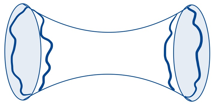
(b)

Figure 3: The disk (a) and annulus (b) geometries in JT gravity. The blue line represents the ‘wiggles’ due to the boundary dynamics of the Schwarzian theory.

3.2 Matching KS theory with JT gravity

First, we show that the disk and annulus partition functions are obtained using the inverse Laplace transform (3.1) of the free one- and two-point functions (2.47). After that, we match the higher genus contributions for an arbitrary number of boundaries.

The disk.

To obtain the one-point function of $Z(\beta)$ in the KS theory we need to compute the following inverse Laplace transform:

$$\langle Z(\beta)\rangle^{\mathsf{c}}_{\mathsf{KS},0}=\int_{c-i\infty}^{c+i\infty}\frac{dz}{2\pi i}\,\braket{\mathcal{J}(z)}_{0}\,e^{\beta z^{2}}=\int_{c-i\infty}^{c+i\infty}\frac{dz}{2\pi i}\,\omega(z)\,e^{\beta z^{2}}~{}.$$ (3.9)

We see that the KS theory determines the leading term in the genus expansion from the holomorphic one-form, which encodes the complex structure of the spectral curve:

$$\omega(z)dz=y(z)dx(z)=\frac{1}{2\pi}z\sin(2\pi z)dz~{}.$$ (3.10)

Since $\omega(z)$ is regular at $z=0$, we can set $c=0$ and substitute $z\to-iw$, giving:

$$\langle Z(\beta)\rangle^{\mathsf{c}}_{\mathsf{KS},0}=\frac{1}{4\pi^{2}}\int_{-\infty}^{\infty}dw\,w\sinh(2\pi w)\,e^{-\beta w^{2}}=\frac{1}{4\pi^{1/2}\beta^{3/2}}e^{\pi^{2}/\beta}~{}.$$ (3.11)

This expression agrees with the path integral of the disk in JT gravity.

The annulus.

Next, we compute the free two-point function of $Z(\beta)$ in KS theory and match it to the annulus amplitude (3.8). For that we need to compute the inverse Laplace transform of the free bosonic two-point function:

$$\langle Z(\beta_{1})Z(\beta_{2})\rangle^{\mathsf{c}}_{\mathsf{KS},0}=\int_{c-i\infty}^{c+i\infty}\frac{dz}{2\pi i}\frac{dw}{2\pi i}\braket{\mathcal{J}(z)\mathcal{J}(w)}^{\mathsf{c}}_{0}e^{\beta_{1}z^{2}+\beta_{2}w^{2}}~{},$$ (3.12)

where

$$\braket{\mathcal{J}(z)\mathcal{J}(w)}^{\mathsf{c}}_{0}=\mathsf{B}(z,w)=\frac{1}{(z-w)^{2}}+\frac{1}{(z+w)^{2}}~{}.$$ (3.13)

Again, we may rotate the contours to the real axis, and then note that both terms in (3.13) give the same contribution upon sending $w\to-w$ in the second integral. Expanding $(z-w)^{-2}$ as a power series, and using gamma functions to compute the resulting Gaussian moments, it can be shown that the double integral gives:

$$\langle Z(\beta_{1})Z(\beta_{2})\rangle^{\mathsf{c}}_{\mathsf{KS},0}=-\frac{1}{4\pi^{2}}\int_{-\infty}^{\infty}dzdw\,\frac{e^{-\beta_{1}z^{2}-\beta_{2}w^{2}}}{(z-w)^{2}}=\frac{1}{2\pi}\frac{\sqrt{\beta_{1}\beta_{2}}}{\beta_{1}+\beta_{2}}~{}.$$ (3.14)

This matches the Euclidean wormhole contribution in JT gravity.

Higher genus amplitudes.

The higher genus corrections in JT gravity are computed recursively, either using Mirzakhani’s recursion for the Weil-Petersson volumes $V_{g,n}(\bm{\ell})$, or, after a Laplace transform, using Eynard and Orantin’s topological recursion. In the KS theory, we can also compute higher-order corrections to connected correlation functions of $\mathcal{J}(z)$ using the SD equation (2.46). We show that the topological recursion is retrieved as the perturbative expansion of the SD equation.

Let us denote the connected correlation functions by

$$\mathcal{W}_{n}(z_{1},\dots,z_{n})\equiv\braket{\mathcal{J}(z_{1})\cdots\mathcal{J}(z_{n})}^{\mathsf{c}}_{\mathsf{KS}}=\frac{\delta^{n}W_{\mathsf{KS}}}{\delta\mu_{\mathcal{J}}(z_{1})\cdots\delta\mu_{\mathcal{J}}(z_{n})}\Big{|}_{\mu_{\mathcal{J}}=0}~{}.$$ (3.15)

We can expand the free energy $W_{\mathsf{KS}}[\mu_{\mathcal{J}}]$ of the KS theory in terms of connected correlation functions as:

$$W_{\mathsf{KS}}[\mu_{\mathcal{J}}]=\sum_{n=0}^{\infty}\int\prod_{i=1}^{n}dz_{i}\frac{\mu_{\mathcal{J}}(z_{1})\cdots\mu_{\mathcal{J}}(z_{1})}{n!}\mathcal{W}_{n}(z_{1},\dots,z_{n})~{}.$$ (3.16)

Plugging this expansion in to the SD equation (2.46) and comparing powers of $\mu_{\mathcal{J}}$, the SD equation takes the form:

$$\mathcal{W}_{n+1}(z_{0},z_{I})=\frac{\lambda}{4}\oint_{\gamma}\frac{dz}{2\pi i}\,\frac{\braket{\mathcal{J}(z_{0})\Phi(z)}_{0}}{\omega(z)}\Big{[}\mathcal{W}_{n+2}(z,z,z_{I})+\sum_{J_{1}\sqcup J_{2}=I}\mathcal{W}_{1+|J_{1}|}(z,z_{J_{1}})\mathcal{W}_{1+|J_{2}|}(z,z_{J_{2}})\Big{]}~{}.$$ (3.17)

The sum in (3.17) is over subsets $J_{1}\sqcup J_{2}=I=\{1,\ldots,n\}$, and the multi-index notation is given by $z_{J}\equiv(z_{j})_{j\in J}$. Next, consider the perturbative expansion in powers of the KS coupling constant $\lambda$:

$$\mathcal{W}_{n}(z_{1},\dots,z_{n})=\sum_{g=0}^{\infty}\lambda^{2g-2+n}\mathcal{W}_{g,n}(z_{1},\dots,z_{n})~{}.$$ (3.18)

Substituting this into (3.17) and matching the terms with the same powers of $\lambda$ we obtain a system of recursive equations:

$$\mathcal{W}_{g,n+1}(z_{0},z_{I})=\underset{z\to 0}{\text{Res}}\,\, \mathcal{K}(z_{0},z)\Big{[}\mathcal{W}_{g-1,n+2}(z,z,z_{I})$$

$$+\sum_{h=0}^{g}\sum^{\prime}_{J_{1}\sqcup J_{2}=I}\mathcal{W}_{h,1+|J_{1}|}(z,z_{J_{1}})\mathcal{W}_{g-h,1+|J_{2}|}(z,z_{J_{2}})\Big{]}~{}.$$ (3.19)

Here, we have defined the recursion kernel $\mathcal{K}(z_{0},z)$ in terms of the twisted propagator as:

$$\mathcal{K}(z_{0},z)\equiv\frac{\braket{\mathcal{J}(z_{0})\Phi(z)}_{0}}{4\,\omega(z)}=\frac{1}{2}\left(\frac{1}{z_{0}-z}-\frac{1}{z_{0}+z}\right)\frac{1}{2\omega(z)}~{},$$ (3.20)

where $\omega(z)=\frac{1}{2\pi}z\sin(2\pi z)$. The prime indicates that terms involving $(g,n)=(0,1)$ should be excluded from the summation. We have replaced the contour integral around the branch point by a residue at $z=0$. The recursion relation is therefore determined by the pole structure of the correlation functions in the complex plane.

Importantly, the recursion in (3.19) corresponds precisely to the topological recursion relations applied to the spectral curve $\mathcal{S}_{\mathrm{JT}}$, with input data:

$$\mathcal{W}_{0,1}(z)=\omega(z)~{},\hskip 10.0pt\mathcal{W}_{0,2}(z_{1},z_{2})=\mathsf{B}(z_{1},z_{2})~{}.$$ (3.21)

The relevant background for the formalism of topological recursion is summarized in appendices B and C. We can combine this result with Eynard and Orantin’s observation [61] that the Weil-Petersson volumes $V_{g,n}$ are related to the ‘symplectic invariants’ $\mathcal{W}_{g,n}$ by a Laplace transform:

$$\mathcal{W}_{g,n}(z_{1},\dots,z_{n})=\int_{0}^{\infty}\prod_{i=1}^{n}d\ell_{i}\,\ell_{i}\,e^{-z_{i}\ell_{i}}V_{g,n}(\ell_{1},\dots,\ell_{n})~{},\quad(\chi<0)~{}.$$ (3.22)

Using our proposal (3.1) for relating JT to KS, we go to the $\beta$-variable by applying the inverse Laplace transform for each $z_{i}$:

$$\braket{Z(\beta_{1})\cdots Z(\beta_{n})}^{\mathsf{c},(g)}_{\mathsf{KS}} =\int_{c-i\infty}^{c+i\infty}\prod_{i=1}^{n}\frac{dz_{i}}{2\pi i}\,e^{\beta_{i}z_{i}^{2}}\mathcal{W}_{g,n}(z_{1},\dots,z_{n})$$ (3.23)

$$=\int_{0}^{\infty}\prod_{i=1}^{n}d\ell_{i}\,\ell_{i}\,V_{g,n}(\ell_{1},\dots,\ell_{n})\,\int_{-\infty}^{\infty}\prod_{i=1}^{n}\frac{dw_{i}}{2\pi}e^{-\beta_{i}w_{i}^{2}-i\ell_{i}w_{i}}$$ (3.24)

$$=\int_{0}^{\infty}\prod_{i=1}^{n}d\ell_{i}\ell_{i}\,V_{g,n}(\ell_{1},\dots,\ell_{n})Z_{\mathsf{trumpet}}(\beta_{i},\ell_{i})~{}.$$ (3.25)

This indeed agrees with the Euclidean path integral $Z_{g,n}^{\mathsf{c}}(\beta_{1},\dots,\beta_{n})$ in (3.6) for the stable surfaces with $\chi<0$. Multiplying by $\lambda^{2g-2+n}$ and summing over the genus we conclude that the perturbative expansion of the universe field theory matches with the genus expansion of the gravitational path integral. Since all correlation functions can be expressed in terms of connected correlations functions, we see that the full JT gravity $n$-boundary path integral is the $n$-point function of the boundary creation operators $Z(\beta)$:

$$\mathcal{Z}_{\mathrm{JT}}(\beta_{1},\dots,\beta_{n})=\braket{Z(\beta_{1})\cdots Z(\beta_{n})}_{\mathsf{KS}}~{}.$$ (3.26)

Let us emphasize that the right-hand side is a non-gravitational Euclidean path integral with $n$ operator insertions, whereas the left-hand side is the gravitational path integral of JT gravity. We have thus expressed JT gravity as a Euclidean ‘universe field theory’ on the spectral curve. This provides a non-perturbative completion (at least on a formal level) of the topological expansion of the Euclidean JT path integral.

Given the geometric interpretation of the chiral boson $\mathcal{J}(z)$ as describing the quantum fluctuations of the target space geometry around the classical value $\omega(z)$, we can think about the ‘ensemble average’ $\braket{\cdots}_{\mathsf{KS}}$ associated to JT gravity, roughly speaking, as describing an average over background geometries in which the JT string propagates.

4 Non-perturbative effects

Given the KS theory description for JT gravity and its embedding in the B-model topological string theory, we can invoke intuition and tools from string theory to study non-perturbative effects of order $\mathcal{O}(e^{1/\lambda})$ in the universe field theory. We will study the insertion of certain topological D-branes [29, 30, 54, 62] in the target space geometry. Their effect will be doubly non-perturbative in $G_{N}$, as can be seen from the identification $\lambda=e^{-S_{0}}$. These contributions are very interesting from the point of view of gravity, as they form an indirect probe of the discreteness of the spectrum in a candidate microscopic theory.

In section 4.1, we will study non-perturbative effects due to the D-branes. These correspond to fermionic objects in the KS theory. In section 4.2, we will give these D-branes an interpretation in JT gravity as hypersurfaces on which fixed energy boundaries can end. These boundaries are described by a boundary term in the JT gravity action that can be obtained from the standard Dirichlet-type boundary action by a Legendre transform, which on the level of the path integral becomes a Laplace transform. As an application of the D-brane formalism, we will show in section 4.3 how to obtain non-perturbative corrections to the density-density correlator, giving the ‘plateau’ feature of the spectral form factor [63].

4.1 Branes in KS theory

Since the basic KS field is a 2-dimensional chiral boson, we can use the familiar boson-fermion correspondence and introduce the following fermionic fields:

$$\psi(z)=e^{\Phi(z)}~{},\quad\quad\psi^{\dagger}(z)=e^{-\Phi(z)}~{}.$$ (4.1)

The exponentials are normal-ordered by subtracting the OPE singularities of $\Phi(z)\Phi(w)\sim\log(z-w)$ in the expansion of the exponential. These fermionic fields have an interpretation as D-branes in the KS theory. Namely, recall that the spectral curve is embedded in the following non-compact Calabi-Yau:

$$\mathsf{CY}:\quad uv-y^{2}+\frac{1}{(4\pi)^{2}}\sin^{2}(2\pi\sqrt{x})=0~{}.$$ (4.2)

The base of this Calabi-Yau is the spectral curve $\mathcal{S}_{\mathrm{JT}}$. This is where the bosonic fields $\mathcal{J}$ and $\Phi$ live. The fibers over the spectral curve are defined by $u=0$ and $v=0$: if we specify a base point on $\mathcal{S}_{\mathrm{JT}}$ these are complex one-dimensional manifolds in the geometry, which can be wrapped by topological D2-branes. In the topological string terminology, $u=0$ is wrapped by a brane, while a brane that wraps the transverse fiber $v=0$ has opposite flux and can be thought of as an ‘anti-brane’ [66]. The fibers are parametrized by a point on the spectral curve, so we can talk about a brane ‘inserted’ at a point $\zeta\in\mathcal{S}_{\mathrm{JT}}$.

In the topological string B-model, integrating out open strings ending on the brane deforms the geometry in which the closed strings propagate [27]. This can be thought of as the backreaction of a brane on the geometry, which deforms the complex structure of $\mathsf{CY}$. As before, the change in complex structure is encoded in the period integral of the holomorphic $(3,0)$-form $\Omega_{\mathsf{CY}}$ around a 3-cycle $\widetilde{C}$ surrounding the D-brane. The change in complex structure due to a single D-brane is found to be [57]:

$$\delta\int_{\widetilde{C}}\Omega_{\mathsf{CY}}=\lambda~{}.$$ (4.3)

We can follow the same steps as in (2.7) to reduce the period integral on the complex 3-cycle surrounding the 2-dimensional brane to a period integral of $\omega$ on a contour $C(\zeta)$ surrounding the point $\zeta$. The result is simply:

$$\delta\oint_{C(\zeta)}\omega=\lambda~{}.$$ (4.4)

What this equation is saying is that the insertion of a brane above the point $\zeta$ deforms the complex structure of the spectral curve $\mathcal{S}_{\mathrm{JT}}$ by a small amount $\lambda$. This is implemented in the quantum theory by a field $\psi(\zeta)$. Rescaling $\omega\to\omega/\lambda$, the property (4.4) can be written as an operator product, to be read inside correlation functions:

$$\oint_{C(\zeta)}dz\,\partial\Phi(z)\,\psi(\zeta)=\psi(\zeta)~{}.$$ (4.5)

We used the defining relation $\delta\omega=d\Phi$ for the chiral boson $\Phi$. We now recognize the operator product expansion of a complex fermion of conformal weight $h=\frac{1}{2}$ with the holomorphic bosonic current $\mathcal{J}(z)=\partial\Phi(z)$:

$$\partial\Phi(z)\psi(\zeta)\sim\frac{1}{z-\zeta}\psi(\zeta)~{}.$$ (4.6)

Conversely, we can obtain $\mathcal{J}(z)$ by taking the coincident limit of a brane and an anti-brane:

$$\partial\Phi(z)=\lim_{z^{\prime}\to z}\Big{\{}\psi(z^{\prime})\psi^{\dagger}(z)\Big{\}}~{}.$$ (4.7)

The accolades signify normal ordering, by subtracting the OPE divergence $\sim\frac{1}{z^{\prime}-z}$. We conclude that the non-compact D-branes described above are indeed nothing but complex fermions on the spectral curve.

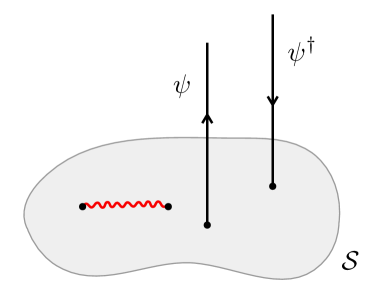
Figure 4: A pictorial representation of non-compact D-brane insertions on the spectral curve $\mathcal{S}$. The straight lines correspond to the non-compact fiber directions $u=0$ or $v=0$ which are wrapped by branes $\psi$ and anti-branes $\psi^{\dagger}$ respectively, having opposite flux as indicated by the direction of the arrow. The branch cut is denoted by a red wiggly line.

So far, we have defined the fermions on the double cover, which is also how we have presented the KS theory. However, ultimately we will be interested in extracting non-perturbative information from the fermions to correlation functions of the density of states $\rho(E)$, where $E$ is related to the base space coordinate $x=-E$. In particular, these quantities will be sensitive, at least semiclassically [68], to the branched structure of the spectral curve. Therefore, we also want to define fermionic fields $\psi(x)$ on the spectral plane $x=z^{2}$. However, this requires us to choose a branch of $z=\sqrt{x}$. We therefore use the formalism developed in [69] to describe $\mathbb{Z}_{2}$-twisted fermions on sheeted Riemann surfaces. To connect to the $\mathbb{Z}_{2}$-twisted boson formalism outlined in appendix C, we will use the spectral plane variable $x$, and obtain physical quantities like $\rho(E)$ by evaluating at $x=-E$ in the end.

4.1.1 $\mathbb{Z}_{2}$-twisted fermions

We think of the spectral curve as two copies of the spectral $x$-plane, glued together along the branch cut on the negative real axis. On each sheet, labelled by indices $0,1$, we define a bosonic field, such that after a $2\pi i$ rotation the fields are rotated into each other:

$$\Phi_{0}(e^{2\pi i}x)=\Phi_{1}(x)~{},\quad\Phi_{1}(e^{2\pi i}x)=\Phi_{0}(x)~{}.$$ (4.8)

In appendix C.6, we introduce explicit mode expansions for $\Phi_{0}$ and $\Phi_{1}$ and show that the KS field $\Phi(x)$ is the combination that diagonalizes the monodromy:

$$\Phi(x)=\frac{1}{\sqrt{2}}(\Phi_{0}(x)-\Phi_{1}(x))~{},\quad x\in\mathbb{C}\setminus\mathbb{R}_{\leq 0}~{}.$$ (4.9)

Then, $\Phi(e^{2\pi i}x)=-\Phi(x)$, so $\Phi$ is indeed an odd function of $z$. In terms of $x$, it has an expansion in only half-integer powers of $x$. So in particular it has a discontinuity across the branch cut, which we will call $\Omega(x)$. The discontinuity can be expressed alternatively in terms of the fields on opposite sheets as they approach each other on the negative real axis:

$$\Omega(x)\equiv\lim_{x^{\prime}\to x}(\Phi_{0}(x)-\Phi_{1}(x^{\prime}))~{},\quad x\in\mathbb{R}_{\leq 0}~{}.$$ (4.10)

Next, on each sheet we introduce the following bosonized fermions:

$$\psi_{a}(x)=\mathsf{c}_{a}e^{\Phi_{a}(x)}~{},\quad\psi_{a}^{\dagger}(x)=\mathsf{c}_{a}e^{-\Phi_{a}(x)}~{},\quad a=0,1~{}.$$ (4.11)

Again, the exponentials are implicitly normal ordered by subtracting the divergences. Furthermore, we have used what is known as the Jordan-Wigner trick to multiply the vertex operators by a cocycle $\mathsf{c}_{a}$ that ensures the correct anti-commutation between fermions on opposite sheets [70]. A consistent choice of cocycles in this case is simply:

$$\mathsf{c}_{0}=1~{},\quad\mathsf{c}_{1}=(-1)^{N_{f}+1}~{},$$ (4.12)

where $N_{f}$ is the fermion number operator. This ensures that fermions on opposite sheets anti-commute, for example:

$$\psi^{\dagger}_{0}(x)\psi_{1}(x^{\prime}) =e^{-\Phi_{0}(x)}(-1)^{N_{f}+1}e^{\Phi_{1}(x^{\prime})}=-\psi_{1}(x^{\prime})\psi^{\dagger}_{0}(x)~{}.$$ (4.13)

For fields on the same sheet, the cocycles square to one and the anti-commutation is ensured by the OPE:

$$\psi_{a}(x)\psi_{b}^{\dagger}(x^{\prime})\sim\frac{\delta_{ab}}{x-x^{\prime}}+\mathrm{reg.}$$ (4.14)

This is of course the expected OPE for fermion fields. As before, we have a boson-fermion correspondence for fermions on the same sheet:

$$\partial\Phi_{a}(x)=\lim_{x^{\prime}\to x}\big{\{}\psi_{a}(x^{\prime})\psi_{a}^{\dagger}(x)\big{\}}\equiv\lim_{x^{\prime}\to x}\left(\psi_{a}^{\dagger}(x^{\prime})\psi_{a}(x)-\frac{1}{x^{\prime}-x}\right)~{}.$$ (4.15)

On the other hand, for two fermions on opposite sheets, we do not have to normal order since $\Phi_{0}(x^{\prime})\Phi_{1}(x)$ is regular, and we can simply add the exponentials in a single normal-ordered exponential:

$$\psi_{0}(x)\psi_{1}^{\dagger}(x)\equiv\lim_{x^{\prime}\to x}\psi_{0}(x^{\prime})\psi^{\dagger}_{1}(x)=\mathsf{c}_{0}\mathsf{c}_{1}\,e^{\Phi_{0}(x)-\Phi_{1}(x)}~{}.$$ (4.16)

Usually for OPE’s we implicitly demand the radial ordering $|x^{\prime}|>|x|$. But here we should be careful about the ordering of the $x$-arguments when we take the coincident limit, since the points are on different sheets. We choose the convention that $\psi_{0}(x^{\prime})$ is always left of $\psi_{1}(x)$ when we take the coincident limit. With this convention, the product of fields when they approach each other from opposite sheets gives the following weight one vertex operators:

$$e^{\Omega(x)}=\lim_{x^{\prime}\to x}\psi_{0}(x^{\prime})\psi_{1}^{\dagger}(x)~{},\quad e^{-\Omega(x)}=\lim_{x^{\prime}\to x}\psi_{0}^{\dagger}(x^{\prime})\psi_{1}(x)~{}.$$ (4.17)

These operators will play an important role in the next section. The fermions have the following monodromies when going around the branch point:

$$\bra{\sigma}\psi_{0}(e^{2\pi i}x)=-\bra{\sigma}\psi_{1}(x)~{},\quad\bra{\sigma}\psi_{1}(e^{2\pi i}x)=-\bra{\sigma}\psi_{0}(x)~{}.$$ (4.18)

We have multiplied from the left by the free bosonic twisted vacuum $\bra{\sigma}$, so that the cocycles $\mathsf{c}_{0},\mathsf{c}_{1}$ become $\pm 1$, respectively. However, from now on we will leave the left-vacuum implicit. This is justified because, as we will see, to extract the non-perturbative physics we will not need the higher genus corrections from the interacting $\ket{\mathsf{KS}}$ vacuum; we will only need the free vacuum $\ket{\sigma}$ correlation functions.

4.2 Interpretation in JT gravity

To connect the discussion of branes on the spectral curve to JT gravity, we should introduce a type of boundary directly in the gravitational theory which can end on branes in the target space geometry. We will thus introduce a set of boundary conditions for the JT universes which do not have a fixed length, but are ‘hovering’ in the bulk at some finite distance, and which have a fixed energy $E$. The observables in the matrix model can now be obtained from the JT path integral with this choice of modified boundary conditions, which on the level of the action amounts to a Legendre transform.

4.2.1 Fixed energy boundary conditions

Instead of fixing the dilaton and the boundary metric as in (3.4), one can also impose Dirichlet-Neumann (DN) boundary conditions, in which one fixes both the dilaton and its normal derivative at the boundary, but leave the metric free [55]:

$$\phi_{\partial M}=\frac{\phi_{r}}{\varepsilon}~{},\hskip 20.0pt\partial_{n}\phi_{\partial M}=\frac{\phi_{r}^{\prime}}{\varepsilon}~{}.$$ (4.19)

Here, we have normalized the normal vector $n$, so that $\partial_{n}\phi$ has the same dimensions as $\phi$. In this case, the following boundary action must be added to the bulk JT gravity action:

$$S^{\partial}_{DN}=-\int_{\partial M}du\sqrt{\gamma_{uu}}(\partial_{n}\phi-\phi\mathcal{K})~{}.$$ (4.20)

The DN boundary conditions are related to the standard DD boundary conditions by a Legendre transform. To see this, we rewrite (4.20) in the following form:

$$S^{\partial}_{DN} =\frac{1}{\varepsilon}\int_{\partial M}du\sqrt{\gamma_{uu}}(\phi_{r}-\phi_{r}^{\prime})+\int_{\partial M}du\sqrt{\gamma_{uu}}\,\phi(\mathcal{K}-1)$$

$$=\int_{0}^{\beta}du\sqrt{\gamma_{uu}}\,E+S^{\partial}_{DD}[\gamma]~{}.$$ (4.21)

We have written explicitly a dependence on the boundary metric $\gamma_{uu}$ in the last term, because in the DN action $\gamma$ is kept free. We recognize the Legendre transform, with conjugate variables $\beta$ and

$$E\equiv\frac{\phi_{r}-\phi_{r}^{\prime}}{\varepsilon}~{}.$$ (4.22)

One can show that (4.22) corresponds to a fixed energy $E=\phi_{r}\mathrm{Sch}(x,u)$ in the boundary Schwarzian theory, when $\epsilon\to 0$. Therefore, the input of a particular Dirichlet type boundary in the JT path integral is some temperature $\beta$ describing a canonical ensemble, whereas the input of a Neumann type boundary is some fixed energy $E$ describing a microcanonical ensemble in the boundary theory.

On the level of the path integral, the Legendre transform becomes an inverse Laplace transform [55]:

$$\mathcal{Z}_{\mathrm{JT}}(E)=\int_{c-i\infty}^{c+i\infty}\frac{\mathcal{D}\gamma}{\mathrm{Diff}\,S^{1}}e^{\int_{0}^{\beta}du\sqrt{\gamma_{uu}}\,E}\mathcal{Z}_{\mathrm{JT}}[\gamma]~{}.$$ (4.23)

We will often omit the superscript DN, as it should be clear from using the variable $E$ that we mean the path integral with DN boundary conditions. We can go to a gauge where $\sqrt{\gamma_{uu}}$ is constant, and then we have to divide by $\beta$ to account for the time reparametrization symmetry:

$$\mathcal{Z}_{\mathrm{JT}}(E)=\int_{c-i\infty}^{c+i\infty}\frac{d\beta}{\beta}e^{\beta E}\mathcal{Z}_{\mathrm{JT}}(\beta)~{}.$$ (4.24)

For example, we can compute the DN partition function of the disk (with $\phi_{r}=\frac{1}{2}$) to be

$$Z_{\mathsf{disk}}(E)=\int_{c-i\infty}^{c+i\infty}\frac{d\beta}{\beta}e^{\beta E}\frac{e^{S_{0}}}{4\pi^{1/2}\beta^{3/2}}e^{\pi^{2}/\beta}=\frac{e^{S_{0}}}{8\pi^{4}}\Big{(}2\pi\sqrt{E}\cosh(2\pi\sqrt{E})-\sinh(2\pi\sqrt{E})\Big{)}~{}.$$ (4.25)

Furthermore, the trumpet partition function becomes

$$Z_{\mathsf{trumpet}}(E,\ell)=\int_{c-i\infty}^{c+i\infty}\frac{d\beta}{\beta}e^{\beta E}\frac{1}{\sqrt{4\pi\beta}}e^{-\frac{\ell^{2}}{4\beta}}=\frac{1}{\pi\ell}\sin(\ell\sqrt{E})~{}.$$ (4.26)

Looking at the form of the higher-genus partition functions (3.6), we see that the $\beta$-dependence only comes in via the trumpets. So, the only modification to the perturbative formula of $\mathcal{Z}_{\mathrm{JT}}(E)$ will be to change the integration kernel of the trumpet to its DN counterpart:

$$Z_{g,n}(E_{1},\dots,E_{n})=\frac{1}{\pi}\int_{0}^{\infty}\prod_{i=1}^{n}d\ell_{i}\sin(\ell_{i}\sqrt{E_{i}})V_{g,n}(\ell_{1},\dots,\ell_{n})~{}.$$ (4.27)

The $\ell_{i}$ from the gluing measure has cancelled with the $\ell_{i}$ in the denominator of (4.26). So $Z_{g,n}(E_{1},\dots,E_{n})$ is simply multiple Fourier-type transform of the Weil-Petersson volumes. We must be careful in evaluating these integrals, as the volumes $V_{g,n}$ are polynomials in $\ell_{i}^{2}$ and so the above integral in general is divergent. However, this divergence can be easily regularized, for example by introducing a small exponential regulator.

4.2.2 Relation to matrix integrals

The fixed energy JT partition function $\mathcal{Z}_{\mathrm{JT}}(E)$ has a direct interpretation in the dual matrix model. To see this, one can write $\mathcal{Z}_{\mathrm{JT}}(\beta)$ as the difference of two integrals in spectral plane coordinate $x=z^{2}$ just above and below the negative real axis:

$$\mathcal{Z}_{\mathrm{JT}}(\beta)=-\lim_{\epsilon\to 0}\int_{-\infty}^{0}\frac{dx}{2\pi i}e^{\beta x}\Big{[}\braket{\partial\Phi(x+i\epsilon)}_{\mathsf{KS}}-\braket{\partial\Phi(x-i\epsilon)}_{\mathsf{KS}}\Big{]}~{}.$$ (4.28)

To obtain $\mathcal{Z}_{\mathrm{JT}}(E)$ from this expression, we use the following integral representation of the delta function:

$$\delta(E+x)=\int_{-i\infty}^{i\infty}d\beta\,e^{\beta(E+x)}~{}.$$ (4.29)

Sending $x\to-x$, the DN path integral can be expressed in terms of KS field insertions as:

$$\mathcal{Z}_{\mathrm{JT}}(E) =\lim_{\epsilon\to 0}\int^{E}dE^{\prime}\int_{0}^{\infty}\frac{dx}{2\pi i}\delta(E^{\prime}-x)\Big{[}\braket{\partial\Phi(-x+i\epsilon)}_{\mathsf{KS}}-\braket{\partial\Phi(-x-i\epsilon)}_{\mathsf{KS}}\Big{]}~{}.$$ (4.30)

Since $E^{\prime}\in\mathbb{R}_{\geq 0}$, the delta function sets $x=E^{\prime}$. From now on we use the short-hand notation $\partial\Phi(E)\equiv\partial\Phi(x)|_{x=-E}$, when $\partial\Phi$ is viewed as a function of $E$. This amounts to moving the branch cut to the positive real axis. On the right-hand side we then recognize the discontinuity of $\partial\Phi$ across the branch cut:

$$\mathrm{disc}\,\partial\Phi(E)\equiv\frac{1}{2\pi i}\lim_{\epsilon\to 0}\Big{(}\braket{\partial\Phi(E+i\epsilon)}_{\mathsf{KS}}-\braket{\partial\Phi(E-i\epsilon)}_{\mathsf{KS}}\Big{)}~{}.$$ (4.31)

We find that $\partial\Phi(E)$ plays the role of the resolvent and its discontinuity across the branch cut is the density of states. Therefore, we will match our notation with that from double-scaled matrix models and write:

$$\rho(E) \equiv\mathrm{disc}\,\partial\Phi(E)~{},\qquad E\in\mathbb{R}_{\geq 0}~{},$$ (4.32)

$$R(E) \equiv\partial\Phi(E)~{},\qquad E\in\mathbb{C}\setminus\mathbb{R}_{\geq 0}~{}.$$ (4.33)

The DN path integral can now be expressed as an insertion of the integrated density of states:

$$Z(E)\equiv\int^{E}dE^{\prime}\,\rho(E^{\prime})~{}.$$ (4.34)

These are the analogues of the boundary creation operators (3.1) in the case of DN boundary conditions. To be precise, we can obtain the JT path integral with DN boundary conditions by inserting these observables in the KS theory:

$$\mathcal{Z}_{\mathrm{JT}}(E_{1},\ldots,E_{n})=\braket{Z(E_{1})\cdots Z(E_{n})}_{\mathsf{KS}}~{}.$$ (4.35)

This completes the dictionary between JT gravity with DN boundary conditions and the KS theory.

\begin{overpic}[width=256.0748pt]{summary1} \put(33.0,50.0){$Z(\beta_{2})$} \put(5.0,50.0){$Z(\beta_{1})$} \put(58.0,43.0){$Z(E_{1})$} \put(87.0,43.0){$Z(E_{2})$} \end{overpic}

Figure 5: The creation of DD and DN boundary trumpets $Z(\beta)$ and $Z(E)$ in JT gravity, indicated by blue and yellow boundaries respectively.

For example, the one-point function $\braket{\partial\Phi(x)}_{\mathsf{KS},0}=\omega(x)$ becomes the leading order density of states:

$$\rho_{0}(E)\equiv\mathrm{disc}\,\omega(E)=\frac{1}{4\pi^{2}}\sinh(2\pi\sqrt{E})~{}.$$ (4.36)

Note that it has the correct universal $\sqrt{E}$-behaviour for low energy, typical of double-scaled matrix models. Integrating, we obtain the disk contribution to the DN path integral, which agrees with our previous answer (4.25):

$$Z_{\mathsf{disk}}(E)=\int^{E}dE^{\prime}e^{S_{0}}\braket{\mathrm{disc}\,\partial\Phi(E^{\prime})}_{\mathsf{KS},0}=\frac{e^{S_{0}}}{8\pi^{4}}\Big{(}2\pi\sqrt{E}\cosh(2\pi\sqrt{E})-\sinh(2\pi\sqrt{E})\Big{)}~{}.$$ (4.37)

Note that the $E$-integral came from the factor of $1/\beta$ present in the definition of the microcanonical path integral. It arose from gauge fixing the $U(1)$ symmetry of trumpet boundary. If we had assumed some marked point on the DN boundary, there would be no such factor of $1/\beta$, and $\mathcal{Z}_{\mathrm{JT}}(E)$ would be computed from insertions of $\rho(E)$. Such operators were considered from the matrix model point of view in [12], where they were called ‘energy eigenbranes’, because they fix a particular energy eigenvalue in the matrix integral.

As another example, we can easily evaluate the contribution from two fixed energy boundaries connected by a wormhole. We do this by glueing two DN trumpets along their common geodesic boundary:

$$\int_{0}^{\infty}d\ell\,\ell\,Z_{\mathsf{trumpet}}(E_{1},\ell)Z_{\mathsf{trumpet}}(E_{2},\ell)=\frac{1}{2\pi^{2}}\log\left(\frac{\sqrt{E_{1}}+\sqrt{E_{2}}}{\sqrt{E_{1}}-\sqrt{E_{2}}}\right)~{}.$$ (4.38)

As expected, the right-hand side is the discontinuity of the free correlator $\braket{\Phi(E_{1})\Phi(E_{2})}_{0}$. Indeed, one can easily verify that taking derivatives with respect to $E_{1}$ and $E_{2}$, followed by an inverse Laplace transform, precisely returns the universal wormhole contribution (3.14).

We can now borrow the matrix model intuition to understand why we found a twisted bosonic field $\partial\Phi$ to describe JT gravity. We have just seen that the energy $E$ that was fixed as a DN boundary condition, and which is dual to the temperature $\beta$, is related to the spectral plane coordinate as $x=-E$. The branch cut in the spectral $x$-plane is therefore mapped to the positive real axis in the $E$-plane. We can view the branch cut, and therefore the fact that $\partial\Phi$ had to be $\mathbb{Z}_{2}$-twisted, as a direct consequence of a continuous eigenvalue density created by $\rho_{0}(E)$. This is the reason we called $x$ the ‘spectral plane’ in the first place: a path in the $x$-plane represents the spectrum of a double-scaled matrix model. A given DD boundary, for which the temperature is fixed, can be thought of as having an energy that is randomly drawn from a continuous statistical ensemble.

The double-scaled matrix model that gives rise to density of states $\rho_{0}(E)$ can be identified explicitly in the topological string theory setup. In fact, there is a precise way in which a stack of topological D2-branes wrapped around compact cycles in the target space geometry (2.4) give rise to a large $N$ matrix integral, which is dual to the closed string theory [29]. In that sense, the random matrix $H$ that leads to $\rho_{0}(E)$ is describing the open string degrees of freedom associated to this brane configuration. The localization of the open string field theory, which in this case is a 6-dimensional holomorphic Chern-Simons theory associated to the space-filling D6-brane, to a matrix integral can be done explicitly [30] (see also [73]). The notation that was used heuristically in (4.32) and (4.33) can then be understood more formally as a statement of the open/closed duality in topological string theory. Hence, from the perspective of the ‘JT string’ it follows that the double-scaled matrix integral is actually dual to the KS field theory, rather than to JT gravity itself. This gives a new perspective on the role of the matrix ensemble associated to the gravitational path integral.

4.3 Application: spectral correlation functions

Now we apply the formalism introduced in the previous section to extract non-perturbative corrections to the leading-order result for density and density-density correlation functions. First, recall that the density of states $\rho(E)$ is the discontinuity of the resolvent operator:

$$\rho(E)=\frac{1}{2\pi i}(\partial\Phi_{0}(E)-\partial\Phi_{1}(E))~{}.$$ (4.39)

The (first order correction to the) collision of two branes on the same sheet $\psi_{0}(E)\psi^{\dagger}_{0}(E)$ leads to the insertion of a closed string state $\partial\Phi$ as in (4.7). The contribution coming from the interaction of branes on opposite sheets is given by

$$\braket{\psi_{0}(E)\psi^{\dagger}_{1}(E)}_{\mathsf{KS}}=\braket{e^{\Omega(E)}}_{\mathsf{KS}}\approx e^{\frac{2\pi i}{\lambda}\int^{E}dE^{\prime}\rho_{0}(E^{\prime})}~{}.$$ (4.40)

Here, we have used that the operator $\Omega(E)$ can be written as

$$\Omega(E)=2\pi i\int^{E}dE^{\prime}\rho(E^{\prime})~{},$$ (4.41)

and kept only the genus zero contribution to the expectation value. The result is entirely localized at the branch cut, and non-perturbative in the coupling constant. Intuitively, one may think about this quantity as a ‘geometric phase’ that a brane picks up when it is transported around the branch point, see Figure 6.

It turns out that this result captures non-perturbative contributions to the density of states if we add the following corrections to the perturbative expansion:

$$\partial\Phi_{0}(E)_{\textrm{np}} \sim\partial\Phi_{0}(E)+ie^{\Omega(E)}~{},$$ (4.42)

$$\partial\Phi_{1}(E)_{\textrm{np}} \sim\partial\Phi_{1}(E)-ie^{-\Omega(E)}~{}.$$ (4.43)

Crucially, the symbol $\sim$ indicates that the above operator identifications should be read inside perturbative expectation values $\braket{\cdots}_{\mathsf{KS}}$ of the KS theory. This is the whole point of the construction: we are trying to extract non-perturbative physics using perturbative computations. The precise mechanism that underlies the above identifications is still rather mysterious, for now one should view it as an observation. We expect that the answer can be found in the open string theory dual to KS, and we hope to address this in future work.

In terms of the matrix model $\partial\Phi(E)=R(E)$ is the resolvent, so the fermions $\psi(E)=\det(H-E)$ and $\psi^{\dagger}(E)=1/\det(H-E)$ correspond to (inverse) determinant operators. In particular, $\psi^{\dagger}$ has singularities at the real axis and should be regularized. This leads to two fermions $\psi^{\dagger}_{0}$ or $\psi^{\dagger}_{1}$ depending on the sign in the $\pm i\epsilon$ prescription. Taking a single eigenvalue $E$ using the probe brane $\psi^{\dagger}_{0}$ and have it circle the branch point once results in the operator $\psi^{\dagger}_{1}$. In the process, the eigenvalue ‘feels’ the force of the other eigenvalues, which is proportional to the number of eigenvalues given by $\int^{E}\rho_{0}(E^{\prime})dE^{\prime}$, and this effect is captured by the non-perturbative phase in $\braket{\psi_{0}(E)\psi^{\dagger}_{1}(E)}_{\mathsf{KS}}$.

Figure 6: A pictorial representation of (a) the collision of two fermions $\psi_{0}$ and $\psi_{0}^{\dagger}$ on the same sheet, (b) the collision of two fermions $\psi_{0}$ and $\psi_{1}^{\dagger}$ on opposite sheets. Effectively, the latter is obtained from moving the anti-brane around the branch point along the striped line, and then bringing the fermions together on the branch cut (indicated by a red wiggly line).

We now make the following proposal for an observable in the universe field theory that captures non-perturbative corrections to the density of states, by analogy with (4.39):

$$\rho_{\textrm{np}}(E)\sim\frac{1}{2\pi i}(\partial\Phi_{0}(E)_{\textrm{np}}-\partial\Phi_{1}(E)_{\textrm{np}})~{}.$$ (4.44)

The superscript ‘np’ indicates that we have defined an observable which takes the non-perturbative corrections into account. With this proposal for a non-perturbative density of states, we can compute perturbative correlation functions in the KS theory.

Density correlator.

The one-point function of $\rho_{\textrm{np}}(E)$ is computed straightforwardly:

$$\braket{\rho_{\textrm{np}}(E)}_{\mathsf{KS}} \sim\braket{\rho(E)}_{\mathsf{KS}}+\frac{1}{2\pi}\left(\braket{e^{\Omega(E)}}_{\mathsf{KS}}+\braket{e^{-\Omega(E)}}_{\mathsf{KS}}\right)~{}.$$ (4.45)

In principle, we can compute this using the full interacting theory, including all genus corrections, but it turns out that the leading-order result already has the features that we are interested in, so we keep only the ‘disk’ and ‘annulus’ contributions. Clearly, we have

$$\braket{\rho(E)}_{\mathsf{KS}}\approx e^{S_{0}}\rho_{0}(E)~{}.$$ (4.46)

For the other contribution we use the following identity:

$$\braket{e^{\pm\Omega(E)}}_{\mathsf{KS}}\approx\exp\left[\pm\braket{\Omega(E)}^{\mathsf{c}}_{0}+\frac{1}{2}\braket{\Omega(E)^{2}}^{\mathsf{c}}_{0}\right]~{}.$$ (4.47)

The annulus contribution, which should be appropriately normal ordered, can be computed using the twisted two-point functions $\braket{\Phi_{a}(x)\Phi_{b}(x^{\prime})}_{\mathsf{KS}}$:

$$\frac{1}{2}\braket{\Omega(x)^{2}}^{\mathsf{c}}_{0} \equiv\frac{1}{2}\lim_{x^{\prime}\to x}\Big{\langle}\{\Omega(x)\Omega(x^{\prime})\}\Big{\rangle}^{\mathsf{c}}_{0}$$

$$=\lim_{x^{\prime}\to x}\Big{[}\log(\sqrt{x}-\sqrt{x^{\prime}})-\log(\sqrt{x}+\sqrt{x^{\prime}})-\log(x-x^{\prime})\Big{]}$$

$$=\log\frac{1}{4x}~{}.$$ (4.48)

Setting $x=-E$, and putting everything together, we thus find the leading-order result:

$$\braket{\rho_{\textrm{np}}(E)}_{\mathsf{KS}}\approx e^{S_{0}}\rho_{0}(E)-\frac{1}{4\pi E}\cos\left(2\pi\,e^{S_{0}}\int^{E}dE^{\prime}\rho_{0}(E^{\prime})\right).$$ (4.49)

This is the same result found by Saad, Shenker and Stanford [7], who obtained it using matrix model techniques. As one can see, the non-perturbative effects give small oscillations on top of the perturbative leading order density of states $\rho_{0}(E)=\frac{1}{4\pi^{2}}\sinh(2\pi\sqrt{E})$, where the size of the oscillations is controlled by $\lambda=e^{-S_{0}}$.

Density-density correlator.

Next, we want to compute the density-density correlator:

$$\braket{\rho_{\textrm{np}}(E_{1})\rho_{\textrm{np}}(E_{2})}_{\mathsf{KS}}~{}.$$ (4.50)

Of course, there will be the factorized contribution, but we will see that the interesting result comes from the connected contributions, which assemble into the so-called sine-kernel, well-known in the matrix model literature. Expanding the expression, there are many products that we need to compute:

$$\rho_{\textrm{np}}(E_{1})\rho_{\textrm{np}}(E_{2}) =\rho(E_{1})\rho(E_{2})+\frac{1}{2\pi}\rho(E_{1})(e^{\Omega(E_{2})}+e^{-\Omega(E_{2})})+\frac{1}{2\pi}(e^{\Omega(E_{1})}+e^{-\Omega(E_{1})})\rho(E_{2})$$

$$\qquad+\frac{1}{4\pi^{2}}(e^{\Omega(E_{1})}+e^{-\Omega(E_{1})})(e^{\Omega(E_{2})}+e^{-\Omega(E_{2})})~{}.$$ (4.51)

The singularities in the cross-terms of $\rho(E)$ with $e^{\Omega(E)}+e^{-\Omega(E)}$ cancel, while the OPE’s of $e^{\Omega(E_{1})}e^{\Omega(E_{2})}$ and $e^{-\Omega(E_{1})}e^{-\Omega(E_{2})}$ are also regular as $E^{\prime}\to E$. The only singular contributions come from the products $\rho(E_{1})\rho(E_{2})$ and $e^{\pm\Omega(E_{1})}e^{\mp\Omega(E_{2})}$. The first gives the perturbative contribution, keeping only the genus zero terms:

$$\braket{\rho(E_{1})\rho(E_{2})}_{\mathsf{KS}} \approx-\frac{1}{2\pi^{2}(E_{1}-E_{2})^{2}}+\mathrm{reg.}$$ (4.52)

where we have neglected terms which are regular as $E^{\prime}\to E$. This perturbative contribution to the density-density correlator is called the ‘ramp’, because after a double Fourier transform it gives rise to the linear growth of the spectral form factor. To obtain the second term, we compute the product:

$$e^{\Omega(E_{1})}e^{-\Omega(E_{2})}=\frac{1}{(E_{1}-E_{2})^{2}}\big{\{}e^{\Omega(E_{1})-\Omega(E_{2})}\big{\}}~{}.$$ (4.53)

Here, we combined the product of normal-ordered exponentials into a single normal-ordered exponential, with the normal ordering $\{\dots\}$ given by subtracting $\log(E_{1}-E_{2})$ from the singular products $\Phi_{0}\Phi_{0}$ and $\Phi_{1}\Phi_{1}$, leading to the multiplicative factor. Now we can take the expectation value and keep only the genus zero contributions:

$$\braket{e^{\Omega(E_{1})}e^{-\Omega(E_{2})}}_{\mathsf{KS}}\approx\frac{1}{(E_{1}-E_{2})^{2}}\exp\left[\braket{\Omega(E_{1})-\Omega(E_{2})}_{0}+\frac{1}{2}\Big{\langle}\big{(}\Omega(E_{1})-\Omega(E_{2})\big{)}^{2}\Big{\rangle}^{\mathsf{c}}_{0}\right]~{}.$$ (4.54)

The square in the last term of the exponent should be appropriately normal-ordered by subtracting the singular pieces, as was the case for the density correlator. It can be easily evaluated using the free two-point functions to be:

$$\frac{1}{2}\braket{(\Omega(x)-\Omega(y))^{2}}^{\mathsf{c}}_{0} =\frac{1}{2}\Big{[}\braket{\Omega(x)^{2}}_{0}^{\mathsf{c}}-2\braket{\{\Omega(x)\Omega(y)\}}_{0}^{\mathsf{c}}+\braket{\Omega(y)^{2}}_{0}^{\mathsf{c}}\Big{]}$$

$$=\log\frac{1}{4x}+\log\frac{1}{4y}-2\left[\log\left(\frac{\sqrt{x}-\sqrt{y}}{\sqrt{x}+\sqrt{y}}\right)-\log(x-y)\right]$$

$$=\log\frac{(\sqrt{x}+\sqrt{y})^{4}}{16xy}~{}.$$ (4.55)

Sending $x=-E_{1}$ and $y=-E_{2}$ and plugging this into (4.54), we find:

$$\braket{e^{\Omega(E_{1})}e^{-\Omega(E_{2})}}_{\mathsf{KS}} \approx\frac{1}{(E_{1}-E_{2})^{2}}\frac{(\sqrt{E_{1}}+\sqrt{E_{2}})^{4}}{16E_{2}E_{1}}\,e^{\braket{\Omega(E_{1})-\Omega(E_{2})}_{0}}$$

$$=\left[\frac{1}{(E_{1}-E_{2})^{2}}+\mathrm{reg.}\right]e^{\braket{\Omega(E_{1})-\Omega(E_{2})}_{0}}~{}.$$ (4.56)

In the last line, we again expanded $E_{1}$ around $E_{2}$ and kept only the singular piece. Repeating the calculation above we find the other OPE with signs flipped:

$$\braket{e^{-\Omega(E_{1})}e^{\Omega(E_{2})}}_{\mathsf{KS}}\approx\left[\frac{1}{(E_{1}-E_{2})^{2}}+\mathrm{reg.}\right]e^{-\braket{\Omega(E_{1})-\Omega(E_{2})}_{0}}~{}.$$ (4.57)

Putting everything together gives the connected contribution to the non-perturbative density-density correlator:

$$\braket{\rho_{\textrm{np}}(E_{1})\rho_{\textrm{np}}(E_{2})}^{\mathsf{c}}_{\mathsf{KS}} \sim\braket{\rho(E_{1})\rho(E_{2})}_{\mathsf{KS}}+\frac{1}{4\pi^{2}}\left(\braket{e^{\Omega(E_{1})}e^{-\Omega(E_{2})}}_{\mathsf{KS}}+\braket{e^{-\Omega(E_{1})}e^{\Omega(E_{2})}}_{\mathsf{KS}}\right)$$

$$\approx-\frac{1}{2\pi^{2}(E_{1}-E_{2})^{2}}\Big{[}1-\cosh\left(\braket{\Omega(E_{1})-\Omega(E_{2})}_{0}\right)\Big{]}~{}.$$ (4.58)

Using that $\braket{\Omega(E)}_{0}=\frac{2\pi i}{\lambda}\int^{E}\rho_{0}(E^{\prime})dE^{\prime}$ we conclude:

$$\braket{\rho_{\textrm{np}}(E_{1})\rho_{\textrm{np}}(E_{2})}^{\mathsf{c}}_{\mathsf{KS}}\approx-\frac{1}{\pi^{2}(E_{1}-E_{2})^{2}}\sin^{2}\left(\pi e^{S_{0}}\int^{E_{1}}_{E_{2}}\rho_{0}(E^{\prime})dE^{\prime}\right)~{}.$$ (4.59)

For $E_{2}\to E_{1}$, the integral can be approximated by $(E_{1}-E_{2})\rho(E_{2})$. Adding the disconnected piece, we arrive at the main result of this section:

$$\braket{\rho_{\textrm{np}}(E_{1})\rho_{\textrm{np}}(E_{2})}_{\mathsf{KS}}\approx\braket{\rho_{\textrm{np}}(E_{1})}_{0}\braket{\rho_{\textrm{np}}(E_{2})}_{0}-\frac{1}{\pi^{2}(E_{1}-E_{2})^{2}}\sin^{2}\!\left(\pi e^{S_{0}}(E_{1}-E_{2})\rho_{0}(E_{2})\right)~{}.$$ (4.60)

This is only an approximate answer, in the sense that we only considered genus zero contributions and were interested in the singular part of the products. The above computation was merely meant to show the universal behaviour of $\braket{\rho(E_{1})\rho(E_{2})}_{\mathsf{KS}}$ for $|E_{1}-E_{2}|\ll 1$. Here, we have shown that the non-perturbative contributions in the universal form of the sine-kernel can be understood as arising from branes in the KS theory. From the universe field theory side, these are described by (bilinears of) fermion fields, while on the JT gravity side, they describe D-branes where fixed-energy boundaries can end on.

5 Discussion

Let us now discuss some subtleties, open questions and directions for future research.

Open/closed duality.

We have proposed that the modified holographic dictionary which relates JT gravity to a matrix integral is in fact a consequence of a more standard open/closed duality in topological string theory. Formulating JT gravity in terms of the KS theory allows for a direct interpretation in string theory and the ‘ensemble average’ should then correspond to the path integral in the open string field theory dual of the KS theory, as outlined in Figure 1. Although we have identified the relevant quantities on both sides, a detailed account of the duality is still an open question. This requires a more careful study of both the compact and non-compact D-branes that we have introduced. More speculatively, we expect that the open string field, which can be represented by a Hermitian matrix $H$, should be viewed as the Hamiltonian of some quantum mechanical system associated to the branes in the theory. It would be interesting to see if the underlying fermionic theory of the open string degrees of freedom can be in some way related to the SYK model [74]. For recent work connecting the SYK model to string theory, see [75].

Baby universes and $\alpha$-states.

Moreover, we expect that the KS theory gives a well-defined construction of the baby universe Hilbert space (as defined in [19]) for JT gravity. One can formally represent the path integral of KS theory in terms of an operator formalism. This would naturally lead to a notion of boundary operators $\widehat{Z}(\beta)$. In fact, we expect a slight modification of the construction by Marolf and Maxfield [19] in the sense that we need to consider a larger algebra of observables by adding the ‘canonical momentum’ of $\widehat{Z}(\beta)$. We would then have a non-commutative algebra of observables with not only boundary creation operators but also boundary annihilation operators. This is close to the original approach taken in [20]. In particular, this construction would lead to a precise definition of the Hartle-Hawking state $\ket{\mathrm{HH}}$ with non-trivial topology, in terms of the interacting vacuum of the KS theory. We can represent this state geometrically by an integration over half the spectral curve. That is, we cut open the path integral on the slice $\mathrm{Re}(z)=0$. The resulting baby universe Hilbert space is infinite-dimensional and distinct from the baby universe Hilbert space that will be discussed in appendix C, since the in- and out-states are treated symmetrically. In principle, this construction would give us a definition of the microscopic $\alpha$-states $|\alpha\rangle$ in JT gravity, and an understanding of their role in the factorization problem [76].

Non-perturbative effects.

It would be interesting to study further the non-perturbative effects that were touched upon in section 4. Although it seems that the brane/anti-brane perspective leads to the correct results (4.49) and (4.60), the geometrical interpretation of the precise mechanism is still rather mysterious. For example, the non-perturbative correction in (4.42) and (4.43) decouples the the two fields $\partial\Phi_{0}$, and $\partial\Phi_{1}$ in the sense that they are not anymore related to each other by a $2\pi$ rotation. This seems to agree with the perspective that non-perturbative effects have a dramatic effect on the target space decoupling the two sheets of the branched geometry [68]. In particular, it leads to a branch cut extending over the whole real axis $[-\infty,\infty]$. It would also be interesting to understand the connection to [77], where an effective field theory for the late-time behaviour of quantum chaotic systems is presented (see also [78]). For example, one could try to find an interpretation of the Altshuler-Andreev saddle and notion of causal symmetry breaking, that are important in the computation of the ‘plateau’ feature of the spectral form factor, in the topological string theory setup. We expect these effects to become visible in the open string field theory description dual to KS theory. This is work in progress.

Super JT gravity.

There are some generalizations of the construction which are worth studying. It would be interesting to carry out a similar analysis in the case of JT supergravity [10, 79]. It is defined on super Riemann surfaces for which a recursion relation similar to Mirzakhani’s is derived. The topological recursion for the matrix model associated to super JT is related to the Brezin-Gross-Witten and the Bessel model [80]. Introducing both fermions and bosons, the super-Virasoro algebra generated by the combined stress tensor leads to super-Virasoro constraints [81]. A natural question is if these are equivalent to the ‘super-Mirzakhani recursion’ and if we can extend the KS theory to a supersymmetric model, whose SD equations impose the super-Virasoro constraints.

$\overline{J}T$-deformation.

Another interesting perspective on the KS interaction (2.36) is as a hybrid between a marginal deformation with the stress tensor and a $T\bar{T}$-deformation. Namely, we have deformed the free theory by an irrelevant operator proportional to $\overline{\partial}\Phi\,T$. Denoting $\overline{\partial}\Phi$ as the anti-holomorphic current $\overline{\mathcal{J}}$, we could call the KS interaction a ‘$\overline{\mathcal{J}}T$-deformation’, by analogy with $T\bar{T}$ [82, 83]. There has been much recent attention for irrelevant deformations similar to $T\bar{T}$ (see, e.g., [84, 85, 86, 87]) and their relation to integrable systems [88, 89, 90, 91], as well as their relation to JT gravity [92, 93]. It would be nice to understand how this discussion fits in.

Pure 3d gravity as an ensemble.

The precise form of the KS action and its relation to JT gravity relied heavily on the interpretation of the spacetime in terms of a string world-sheet. In that sense, the construction seems to be very specific to models of 2-dimensional gravity. There is some evidence that wormholes in pure 3-dimensional gravity can also be understood in terms of some averaging prescription (research in this direction includes [16, 94, 95, 96, 97, 98, 99, 100]). Our derivation was fundamentally based on the universal recursive structure expressed in terms of the SD equation. If one could unearth a similar recursive structure in higher-dimensional theories of quantum gravity, this would open up a way for finding a similar field theory description.

We hope to address some of these questions in future work.

Appendix A Free two-point functions of the universe field theory

We compute the two-point functions of the free theory including sources (2.21) with action (2.18). The partition function is just a Gaussian integral in $\Phi$ and $\mathcal{J}$, so we can solve it by functional determinants. We will start with the $\Phi$-integral. Integrating by parts, the terms involving $\Phi$ are:

$$\frac{1}{2}\Phi\,\partial\overline{\partial}\,\Phi-\Phi\,\overline{\partial}\mathcal{J}-\mu_{\Phi}\Phi~{}.$$ (A.1)

The Laplacian $\Delta=\partial\overline{\partial}$ on the spectral curve has a Green’s function $\Delta^{-1}$, which can be found by first projecting to the spectral $x$-plane, and then transforming back to the double cover via $x=z^{2}$. There is a branch cut on the negative real axis and therefore the Green’s function on the $x$-plane can be found using the method of images [101]. Transforming to the double cover, $x=z^{2},y=w^{2}$, we find the result

$$\Delta^{-1}(z,w)=\frac{1}{2}\ln\left|\frac{z-w}{z+w}\right|~{}.$$ (A.2)

We can now solve the $\Phi$-integral by completing the square:

$$\int[d\Phi]\exp\left[\frac{1}{2}\Phi\,\partial\overline{\partial}\,\Phi-\Phi\,\overline{\partial}\mathcal{J}-\mu_{\Phi}\Phi\right]=N\exp\left[-\frac{1}{2}(\overline{\partial}\mathcal{J}+\mu_{\Phi})\Delta^{-1}(\overline{\partial}\mathcal{J}+\mu_{\Phi})\right]~{}.$$ (A.3)

Here, we have used the condensed notation

$$A\,\Delta^{-1}B\equiv\int d^{2}z\int d^{2}w\,A(z)\Delta^{-1}(z,w)B(w)~{}.$$ (A.4)

We have also denoted the functional determinant by $N$, which is just a (possibly infinite) constant that drops out, because we have normalized the partition function. Explicitly, the functional determinant is

$$N =\int[d\Phi]\exp\left[\frac{1}{2}\Big{(}\Phi-\Delta^{-1}(\mu_{\Phi}+\overline{\partial}\mathcal{J})\Big{)}\Delta\Big{(}\Phi-\Delta^{-1}(\mu_{\Phi}+\overline{\partial}\mathcal{J})\Big{)}\right]$$ (A.5)

$$=\int[d\Phi^{\prime}]\exp\left[-\frac{1}{2}\Phi^{\prime}(-\Delta)\Phi^{\prime}\right]=\det(-\Delta)^{-1}~{}.$$ (A.6)

In general, the determinant should be regularized, but we do not have to worry about this since we have normalized the partition function with sources. Having done the $\Phi$-integral, we are left with the integration over $\mathcal{J}$:

$$Z^{(0)}_{\mathsf{KS}}[\mu_{\Phi},\mu_{\mathcal{J}}]=\frac{N}{Z^{(0)}_{\mathsf{KS}}[0]}\int[d\mathcal{J}]\exp\left[-\frac{1}{2}(\overline{\partial}\mathcal{J}+\mu_{\Phi})\Delta^{-1}(\overline{\partial}\mathcal{J}+\mu_{\Phi})-\mu_{\mathcal{J}}\mathcal{J}\right]~{}.$$ (A.7)

Now we introduce the Green’s function for the $\overline{\partial}$-operator on the spectral curve. It is simply the derivative of the Green’s function in (A.2):

$$\overline{\partial}^{-1}=\partial\Delta^{-1}=\frac{dz}{z-w}-\frac{dz}{z+w}~{}.$$ (A.8)

Writing $\,\overline{\partial}^{-1}\equiv\overline{\partial}^{-1}(z,w)\,dz$, we perform the shift

$$\mathcal{J}\to\mathcal{J}-\overline{\partial}^{-1}\!\cdot\mu_{\Phi}~{},$$ (A.9)

where the $\cdot$ means that we integrate with respect to the second argument of $\overline{\partial}^{-1}$:

$$\overline{\partial}^{-1}\!\cdot\mu_{\Phi}\equiv\int d^{2}w\,\left(\overline{\partial}^{-1}(z,w)\mu_{\Phi}(w)\right)\,dz~{}.$$ (A.10)

The exponent of (A.7) now becomes

$$-\frac{1}{2}\overline{\partial}\mathcal{J}\,\Delta^{-1}\,\overline{\partial}\mathcal{J}-\mu_{\mathcal{J}}\big{(}\mathcal{J}-\overline{\partial}^{-1}\!\cdot\mu_{\Phi}\big{)}~{}.$$ (A.11)

Integrating the first term by parts, and using that $\overline{\partial}\Delta^{-1}=\partial^{-1}$, we see that the free partition function is

$$Z^{(0)}_{\mathsf{KS}}[\mu_{\Phi},\mu_{\mathcal{J}}]=\frac{N}{Z^{(0)}_{\mathsf{KS}}[0]}\int[d\mathcal{J}]\exp\left[\frac{1}{2}\mathcal{J}\,\partial^{-1}\overline{\partial}\mathcal{J}-\mu_{\mathcal{J}}\mathcal{J}\right]\exp\left[\mu_{\mathcal{J}}\overline{\partial}^{-1}\mu_{\Phi}\right]~{}.$$ (A.12)

We can complete the square in the first exponent and do the Gaussian integral, which gives us

$$Z^{(0)}_{\mathsf{KS}}[\mu_{\Phi},\mu_{\mathcal{J}}]=\frac{N\,N^{\prime}}{Z^{(0)}_{\mathsf{KS}}[0]}\exp\left[\frac{1}{2}\mu_{\mathcal{J}}\partial\overline{\partial}^{-1}\mu_{\mathcal{J}}+\mu_{\mathcal{J}}\overline{\partial}^{-1}\mu_{\Phi}\right]~{}.$$ (A.13)

We have written the functional determinant $N^{\prime}$ as

$$N^{\prime} =\int[d\mathcal{J}]\exp\left[\frac{1}{2}\Big{(}\mathcal{J}-(\partial^{-1}\overline{\partial})^{-1}\mu_{\mathcal{J}}\Big{)}\,\partial^{-1}\overline{\partial}\,\Big{(}\mathcal{J}-(\partial^{-1}\overline{\partial})^{-1}\mu_{\mathcal{J}}\Big{)}\right]$$ (A.14)

$$=\int[d\mathcal{J}^{\prime}]\exp\left[-\frac{1}{2}\mathcal{J}^{\prime}(-\partial^{-1}\overline{\partial})\mathcal{J}^{\prime}\right]=\det(-\partial^{-1}\overline{\partial}\,)^{-1}~{}.$$ (A.15)

In arriving at (A.13), we have also used that $(\partial^{-1}\overline{\partial})^{-1}=-\partial\overline{\partial}^{-1}$, as can be verified by acting from the left with $\partial^{-1}\overline{\partial}$ and integrating by parts. The factors $N$ and $N^{\prime}$ cancel against the normalization, as can be seen by turning off the sources. Therefore, we have shown that:

$$Z^{(0)}_{\mathsf{KS}}[\mu_{\Phi},\mu_{\mathcal{J}}]=\exp\left[\frac{1}{2}\mu_{\mathcal{J}}\partial\overline{\partial}^{-1}\mu_{\mathcal{J}}+\mu_{\mathcal{J}}\overline{\partial}^{-1}\mu_{\Phi}\right]~{}.$$ (A.16)

In particular, this implies that there are only contractions between $\mathcal{J}$ and $\mathcal{J}$, and between $\mathcal{J}$ and $\Phi$. There is no contraction of $\Phi$ with itself. Here, $\overline{\partial}^{-1}$ is given by (A.8) and

$$\partial\overline{\partial}^{-1}=\frac{dz\,dw}{(z-w)^{2}}+\frac{dz\,dw}{(z+w)^{2}}~{}.$$ (A.17)

So, if we define the following functions:

$$\mathsf{B}(z,w)=\frac{1}{(z-w)^{2}}+\frac{1}{(z+w)^{2}},\quad\mathsf{G}(z,w)=\frac{1}{z-w}-\frac{1}{z+w}~{},$$ (A.18)

we arrive at the result claimed in the main text:

$$\log Z^{(0)}_{\mathsf{KS}}[\mu_{\Phi},\mu_{\mathcal{J}}]=\int d^{2}z\int d^{2}w\left[\frac{1}{2}\mu_{\mathcal{J}}(z)\mathsf{B}(z,w)\mu_{\mathcal{J}}(w)+\mu_{\mathcal{J}}(z)\mathsf{G}(z,w)\mu_{\Phi}(w)\right]~{}.$$ (A.19)

Appendix B Topological recursion

In this appendix we give some background on the topological recursion formalism of Eynard and Orantin [51, 102]. The starting point of the topological recursion is the data of a spectral curve, which consists of a tuple $(\mathcal{C},x,y,\mathcal{B})$, where

• $\mathcal{C}$ is a compact Riemann surface,

• $x$ and $y$ are two analytical functions on an open domain of $\mathcal{C}$,

• $\mathcal{B}$ is the Bergmann kernel of $\mathcal{C}$, which in local coordinates $z,w$, is the unique bilinear differential with a double pole at $z=w$ and no other poles:

  $$\mathcal{B}(z,w)=\frac{dz\,dw}{(z-w)^{2}}+\mathrm{reg.}\quad\mathrm{as}\quad z\to w~{}.$$ (B.1)

We will consider the case in which $\mathcal{C}$ is (topologically) the Riemann sphere $\mathbb{P}^{1}=\mathbb{C}\cup\{\infty\}$. The functions $x$ and $y$ satisfy a relation of the form $H(x,y)=0$, which defines an (algebraic) curve $\mathcal{S}$, which is also referred to as the spectral curve. The spectral curve $\mathcal{S}$ is a branched cover of the spectral plane given by the $x$-coordinate, with branch points $a_{i}$ defined by $dx(a_{i})=0$. The covering map corresponds to the projection to the $x$-axis, which is two-to-one in the case of JT gravity. The two ‘sheets’ of the double cover are exchanged in the neighbourhood of a branch point by a local involution $z\to\tilde{z}$.

B.1 The spectral curve for JT gravity

We will now describe the spectral curve that is relevant for JT gravity. It is given in terms of the one-point function $\omega(x)=\frac{1}{4\pi}\sin(2\pi\sqrt{x})$ by

$$\mathcal{S}_{\mathrm{JT}}:\quad y^{2}=\omega(x)^{2}~{}.$$ (B.2)

Figure 7: Spectral curve for JT gravity. There is one branch point at $z=0$, corresponding to $x=0$. The involution exchanges $z$ and $\tilde{z}=-z$.

The spectral curve can be parametrized by a single uniformizing coordinate $z\in\mathbb{P}^{1}$:

$$\mathcal{S}_{\mathrm{JT}}:\quad x(z)=z^{2}~{},\quad y(z)=\frac{1}{4\pi}\sin(2\pi z)~{}.$$ (B.3)

A real slice of this curve is plotted in Figure 7. The function $x(z)=z^{2}$ gives $\mathcal{S}_{\mathrm{JT}}$ the structure of a branched double cover of the spectral $x$-plane. There is a single branch point at $z=0$, since $dx=2zdz$. The branch point $z=0$ gets mapped to $x=0$ on the spectral plane. The involution that exchanges the sheets of the double cover is simply $z\to-z$.

It should be noted that the curve $H(x,y)=0$ is not algebraic, since $\omega(x)^{2}$ is not a finite polynomial, so $\mathcal{S}_{\mathrm{JT}}$ is a non-compact Riemann surface. However, since it can be parametrized by a single variable $z\in\mathbb{P}^{1}$ one could possibly add a point at $\infty$, and argue that $\mathcal{S}_{\mathrm{JT}}$ effectively has genus zero. However, the notion of ‘genus’ for such non-compact Riemann surfaces is somewhat vague, and another interesting interpretation of $\mathcal{S}_{\mathrm{JT}}$ is as a Riemann surface of infinite genus of which infinitely many $A$-cycles have been pinched. This interpretation can be justified when we compare to the $(2,p)$-minimal string theory with $p$ an odd integer, studied for example in [103]. In that case, the spectral curve was found to be an odd power $y(z)\sim z^{p}$, so that $H(x,y)=0$ describes a compact Riemann surface of genus $p$. We can thus quite possibly see the JT spectral curve $y(z)\sim\sin(2\pi z)$, being an odd power series in $z$, as a ‘infinite linear combination’ of $(2,p)$-minimal models, as was recently advocated in [13, 14].

The reason that we effectively see a genus zero spectral curve is that all the $A$-cycles have been pinched to points, at the zeros of the $\sin(2\pi z)$ where the two sheets of the double cover meet. Non-perturbative effects may cause the zeroes of $y(z)$ to ‘open up’, adding small corrections to the right-hand side of (B.3) and thereby un-pinching the $A$-cycles. Since $\sin(2\pi z)$ has infinitely many zeroes, this un-pinching renders $\mathcal{S}_{\mathrm{JT}}$ a genus $p\to\infty$ Riemann surface. The $p\to\infty$ limit of minimal string theory was recently studied more thoroughly in [15], where many quantities were matched to quantities in JT gravity.

B.2 The symplectic invariants of TR

The topological recursion associates to the data $(\mathcal{C},x,y,\mathcal{B})$, a set of so-called symplectic invariants $\omega_{g,n}$ on the spectral curve. They are defined recursively, starting from the initial data

$$\omega_{0,1}(z)\equiv y(z)dx(z)~{},\hskip 15.0pt\omega_{0,2}(z_{1},z_{2})\equiv\mathcal{B}(z_{1},z_{2})~{}.$$ (B.4)

The recursion kernel is defined by

$$\mathcal{K}(z_{0},z)\equiv\frac{\frac{1}{2}\int_{\tilde{z}}^{z}\mathcal{B}(z_{0},\,\cdot\,)}{\big{(}y(z)-y(\tilde{z})\big{)}dx(z)}~{}.\vspace{1em}$$ (B.5)

Here, the coordinates $z,w$ and the involution $z\to\widetilde{z}$ are defined locally near a branch point $a_{i}$. Moreover, $\frac{1}{dx(z)}$ denotes the contraction with the vector field $\left(\frac{dx}{dz}\right)^{-1}\partial_{z}$. The notation $\int\mathcal{B}(z_{0},\,\cdot\,)$ means that we integrate only with respect to the second argument. This makes $\mathcal{K}(z_{0},z)$ a tensor of the type $dz_{0}\otimes\partial_{z}$. In other words, when acting on a multilinear differential $dz_{1}\otimes\dots\otimes dz_{n}$, it removes a factor of $dz$ and tensors with $dz_{0}$.

The topological recursion then produces multi-differentials of the form

$$\omega_{g,n}(z_{1},\dots,z_{n})=\mathcal{W}_{g,n}(z_{1},\dots,z_{n})\,dz_{1}\otimes\cdots\otimes dz_{n}~{},$$ (B.6)

which are defined recursively by taking residues at the branch points,

$$\omega_{g,n+1}(z_{0},z_{I}) =\sum_{i}\underset{z\to a_{i}}{\mathrm{Res}}\,\mathcal{K}(z_{0},z)\Big{[}\underbrace{\omega_{g-1,n+2}(z,\widetilde{z},z_{I})}_{{\color[rgb]{0,0,1}b)}}$$

$$\hskip 56.9055pt+\sideset{}{{}^{\prime}}{\sum}_{\begin{subarray}{c}g_{1}+g_{2}=g\\[2.10002pt] J_{1}\sqcup J_{2}=I\end{subarray}}\underbrace{\omega_{g_{1},1+|J_{1}|}(z,z_{J_{1}})\,\omega_{g_{2},1+|J_{2}|}(\widetilde{z},z_{J_{2}})}_{{\color[rgb]{0,0,1}a)+c)}}\Big{]}~{}.$$ (B.7)

We denote $z_{J}=(z_{j})_{j\in J}$ and the sum in the last term goes over all ways to partition the multi-index $I=(i_{1},\dots,i_{n})$ into subsets $J_{1}$ and $J_{2}$, and over all ways to distribute $g$ into $g_{1}+g_{2}$. The prime indicates that terms involving $(g,n)=(0,1)$ should be excluded from the summation. The labels ${\color[rgb]{0,0,1}a)}$, ${\color[rgb]{0,0,1}b)}$ and ${\color[rgb]{0,0,1}c)}$ will be explained momentarily.

B.3 The symplectic invariants for JT gravity

There is a structural similarity between the topological recursion (B.2) and Mirzakhani’s recursion relations [49, 50]. A detailed account of Mirzakhani’s recursion goes beyond the scope of this appendix. For now we are content with a graphical representation of the recursion which expresses the Weil-Petersson volume of a hyperbolic surface in terms of smaller surfaces where a pair-of-pants has been stripped off. The terms appearing on the right-hand side of the topological recursion are packaged in a way similar to Mirzakhani’s recursion, if we identify $g$ and $n$ with the genus and number of boundaries respectively. To make the comparison more transparent, we have labelled the terms by the three scenarios ${\color[rgb]{0,0,1}a)}$, ${\color[rgb]{0,0,1}b)}$ and ${\color[rgb]{0,0,1}c)}$ which are depicted in figure 8. The contact term ${\color[rgb]{0,0,1}a)}$, which corresponds to the joining of two ‘baby universes’, is incorporated in the topological recursion (B.2) as the $(g_{1},g_{2})=(g,0)$ term of the primed sum. At each recursion step, this term is the only one that contains the Bergmann kernel $\mathcal{B}=\omega_{0,2}$.

\begin{overpic}[width=176.91455pt]{chop1}\put(1.0,3.0){$a)$}\end{overpic}

\begin{overpic}[width=159.22578pt]{chop2}\put(1.0,3.0){$b)$}\end{overpic}

\begin{overpic}[width=159.22578pt]{chop3}\put(1.0,3.0){$c)$}\end{overpic}

Figure 8: Graphical representation of the terms in Mirzakhani’s recursion. Stripping off a pair-of-pants from a surface can lead to three scenarios: $a)$ the stripped surface has one boundary less than the original, but the genus stays the same, $b)$ it has one boundary more than the original, but the genus goes down by one, $c)$ the surface splits into two disconnected pieces, $M_{1}\cup M_{2}$, such that the genera and external boundaries get distributed among $M_{1}$ and $M_{2}$.

There is a special case in which the topological recursion is indeed equivalent to Mirzakhani’s recursion. The initial data is precisely the JT spectral curve defined by equation (B.3) with Bergmann kernel given by

$$\mathcal{B}(z_{1},z_{2})=\frac{dz_{1}\,dz_{2}}{(z_{1}-z_{2})^{2}}~{}.$$ (B.8)

Furthermore, $y(\tilde{z})=y(-z)=-y(z)$ so the recursion kernel becomes

$$\mathcal{K}(z_{0},z) =\frac{1}{2}\int_{-z}^{z}\frac{1}{(z_{0}-z^{\prime})^{2}}dz^{\prime}\frac{dz_{0}}{4y(z)zdz}=\frac{1}{z_{0}^{2}-z^{2}}\frac{\pi}{\sin(2\pi z)}dz_{0}\otimes\partial_{z}~{}.$$ (B.9)

We can expand the recursion kernel and take residues at the branch point $z=0$. Since the right-hand side of (B.2) only contains poles of finite order, we only need to keep a finite number of terms in the expansion of $\mathcal{K}(z_{0},z)$.

It was proven that a Laplace transform of Mirzakhani’s recursion gives the topological recursion in the case that the spectral curve is given by (B.3) (the proof can be found in appendix A of [51]). The relation between the Weil-Petersson volumes and the symplectic invariants for general $(g,n)$ is the following multi-Laplace transform:

$$\mathcal{W}_{g,n}(z_{1},\ldots,z_{n})=2^{-\delta_{g,1}\delta_{n,1}}\int_{0}^{\infty}\prod_{i=1}^{n}d\ell_{i}\,\ell_{i}\,e^{-z_{i}\ell_{i}}V_{g,n}(\ell_{1},\ldots,\ell_{n})~{}.$$ (B.10)

Given this relation, one can determine how the symplectic invariants are related to the JT partition functions $Z^{\mathsf{c}}_{g,n}(\beta_{1},\ldots,\beta_{n})$, as was used in the main text.

Appendix C Baby universe Hilbert space and Virasoro constraints

In this appendix, we give another perspective on the duality between KS theory and JT gravity by exploiting the relation to topological gravity, making the underlying Virasoro symmetry manifest. The approach is similar to the SD equation, but makes use of the operator formalism instead of path integrals and should be viewed as complementary. We show that one can reformulate the KS recursion relation in terms of a Virasoro constraint on the partition function, which is also satisfied by the Weil-Petersson volumes (when viewed as intersection numbers of the moduli space). This naturally leads to a definition of a baby universe Hilbert space.

The Weil-Petersson volumes can be expressed in terms of the intersection theory of the moduli space via:

$$V_{g,n}(\bm{\ell})=\int_{\overline{\mathcal{M}}_{g,n}}\exp\Big{(}\Omega_{\mathrm{WP}}+\frac{1}{2}\sum_{i=1}^{n}\psi_{i}\ell_{i}^{2}\Big{)}~{},$$ (C.1)

where $\bm{\ell}=(\ell_{1},\ldots,\ell_{n})$, $\Omega_{\mathrm{WP}}$ is the Weil-Petersson symplectic form on the moduli space and $\psi_{i}$ are $\psi$-classes on the moduli space. See, for example, [34] for more details. Attaching the trumpets (we set $\phi_{r}=1$ in (3.4) for convenience, which is different from the convention used in (3.7)), and using the integral identity $\int_{0}^{\infty}x\exp(-\frac{1}{2}ax^{2})dx=a^{-1}$, we can write the genus $g$ contribution to the JT path integral with $n$ boundaries of lengths $\bm{\beta}=(\beta_{1},\ldots,\beta_{n})$ in the following form:

$$Z^{\mathsf{c}}_{g,n}(\bm{\beta}) =\int_{0}^{\infty}\prod_{i=1}^{n}d\ell_{i}\frac{\ell_{i}}{\sqrt{2\pi\beta_{i}}}e^{-\frac{1}{2}\ell_{i}^{2}/\beta_{i}}\int_{\overline{\mathcal{M}}_{g,n}}e^{\Omega_{\mathrm{WP}}+\frac{1}{2}\psi_{i}\ell_{i}^{2}}$$

$$=\int_{\overline{\mathcal{M}}_{g,n}}e^{\Omega_{\mathrm{WP}}}\int_{0}^{\infty}\prod_{i=1}^{n}d\ell_{i}\frac{\ell_{i}}{\sqrt{2\pi\beta_{i}}}\exp\left(-\frac{1}{2}\left(\beta_{i}^{-1}-\psi_{i}\right)\ell_{i}^{2}\right)$$

$$=\int_{\overline{\mathcal{M}}_{g,n}}e^{\Omega_{\mathrm{WP}}}\prod_{i=1}^{n}\sqrt{\frac{\beta_{i}}{2\pi}}(1-\beta_{i}\psi_{i})^{-1}~{}.$$ (C.2)

We can interpret this result in the following way. When we define JT gravity on hyperbolic surfaces without boundaries (allowing only marked points), we do not need to include any boundary terms in the action. So correlation functions in this theory are simply defined by integrating over the moduli space:

$$\langle\cdots\rangle_{g}=\int_{\overline{\mathcal{M}}_{g,n}}e^{\Omega_{\mathrm{WP}}}(\cdots)~{}.$$ (C.3)

From (C.2) we now see that one can create an asymptotically AdS₂ boundary of renormalized length $\beta$ by inserting the ‘observable’

$$Z(\beta)=\lambda\sqrt{\frac{\beta}{2\pi}}(1-\beta\psi)^{-1}~{}.$$ (C.4)

This point of view is familiar in the context of 2d topological gravity [35, 36, 38]. Note that the observables have an extra factor of $\lambda$ compared to the main text. Summing over the genus counting parameter $\lambda=e^{-S_{0}}$, we can thus think of the JT gravity path integral as the correlation function of ‘boundary creation operators’ $Z(\beta_{i})$ in topological gravity:

$$\mathcal{Z}^{\mathsf{c}}_{\chi<0}(\bm{\beta})=\langle Z(\beta_{1})\cdots Z(\beta_{n})\rangle\sim\sum_{\chi<0}\lambda^{2g-2}\langle Z(\beta_{1})\cdots Z(\beta_{n})\rangle_{g}~{}.$$ (C.5)

The operators $Z(\beta_{i})$ are called macroscopic loop operators in the context of matrix models, see, for instance, [104] (and more recently [32]). We will now make the notation of (C.5) precise, by rewriting $Z(\beta)$ as a creation operator $Z_{+}(\beta)$ in a bosonic Fock space.

C.1 Virasoro constraints

To turn $Z(\beta)$ into a differential operator, we introduce the generating function $F$ for the intersection numbers of $\psi$-classes and the Weil-Petersson symplectic form:

$$F(\bm{t})=\sum_{g=0}^{\infty}\lambda^{2g-2}\int_{\overline{\mathcal{M}}_{g,n}}\exp(\Omega_{\mathrm{WP}}+\sum_{i}t_{i}\sigma_{i})~{},$$ (C.6)

where the $t_{i}$ are ‘sources’ for $\sigma_{d_{i}}\equiv\psi_{i}^{d_{i}}$. Expanding $Z(\beta)$ in a geometric series, we have:

$$Z(\beta)=\lambda\sqrt{\frac{\beta}{2\pi}}\sum_{k=0}^{\infty}(\psi\beta)^{k}=\frac{\lambda}{\sqrt{2\pi}}\sum_{k=0}^{\infty}\sigma_{k}\beta^{k+\frac{1}{2}}~{}.$$ (C.7)

Therefore, we can write the connected JT path integral over the stable surfaces (with $\chi<0$) as differential operators acting on the generating function:

$$\mathcal{Z}^{\mathsf{c}}_{\chi<0}(\bm{\beta})=Z_{+}(\beta_{1})\cdots Z_{+}(\beta_{n})\,F(\bm{t})\,\Big{|}_{\begin{subarray}{c}\bm{t}=0\end{subarray}}~{},$$ (C.8)

where

$$Z_{+}(\beta_{i})=\frac{\lambda}{\sqrt{2\pi}}\sum_{k_{i}=0}^{\infty}\beta_{i}^{k_{i}+\frac{1}{2}}\frac{\partial}{\partial t_{k_{i}}}~{}.$$ (C.9)

We see that $F(\bm{t})$ is the generating function for connected contributions to the JT path integral, and has the interpretation of a ‘free energy’. Therefore, its exponent $e^{F}$ has the interpretation of the full partition function of no-boundary JT gravity. Acting with suitable trumpet creation operators $Z_{+}(\beta_{i})$ on $e^{F}$ thus produces both connected and disconnected contributions to the path integral. The free energy $F$ generates just the spacetime wormholes, whereas $e^{F}$ contains both wormholes and factorized contributions. For example, acting with $Z_{+}(\beta_{1})Z_{+}(\beta_{2})$ on $e^{F}$ produces, graphically, the two contributions in Figure 9.

\begin{overpic}[width=132.68929pt]{connected1} \put(-15.0,24.0){$\sum_{g}$}\end{overpic}

\begin{overpic}[width=84.03677pt]{disconnected1} \put(-31.0,34.0){{$\Huge\Big{(}$}} \put(-43.0,39.0){+} \put(-20.0,39.0){$\sum_{h}$} \put(95.0,34.0){{$\Huge\Big{)}$}} \end{overpic}

\begin{overpic}[width=84.03677pt]{disconnected2} \put(-31.0,34.0){{$\Huge\Big{(}$}} \put(-20.0,39.0){$\sum_{h^{\prime}}$} \put(95.0,34.0){{$\Huge\Big{)}$}} \end{overpic}

Figure 9: Both wormholes and factorized contributions appear in $Z_{+}(\beta_{1})Z_{+}(\beta_{2})\exp F$.

A natural question is how Mirzakhani’s recursion can be rephrased in the operator language that we have just described. Since $F(\bm{t})$ can be used to generate Weil-Petersson volumes, a natural guess would be that the integral recursion relation of Mirzakhani can be written in a differential version as some combination of trumpet creation operators $Z_{+}(\beta_{i})$ acting on the partition function:

$$\widehat{\mathcal{O}}\big{[}\{t_{i},\partial_{t_{i}}\}_{i}\big{]}\,e^{F(\bm{t})}=0~{}.$$ (C.10)

The precise form of the operator $\widehat{\mathcal{O}}$ can be found in [106]. An intermediate result reads:

$$\quad(2k+3)!!\frac{\partial F}{\partial t_{k+1}} =\sum_{i,j=0}^{\infty}\underbrace{\mathcal{F}_{ijk}\,t_{j}\,\frac{\partial F}{\partial t_{i+j+k}}}_{{\color[rgb]{0,0,1}a)}}$$

$$+\frac{\lambda^{2}}{4}\sum_{i=0}^{\infty}\sum_{\begin{subarray}{c}j_{1}+j_{2}=\\ i+k-1\end{subarray}}\widetilde{\mathcal{F}}_{i\,j_{1}j_{2}}\Big{(}\underbrace{\frac{\partial^{2}F}{\partial t_{j_{1}}\partial t_{j_{2}}}}_{{\color[rgb]{0,0,1}b)}}+\underbrace{\frac{\partial F}{\partial t_{j_{1}}}\frac{\partial F}{\partial t_{j_{2}}}}_{{\color[rgb]{0,0,1}c)}}\Big{)}\qquad\forall\,k>0~{}.$$ (C.11)

The coefficients are given by:

$$\mathcal{F}_{ijk}=\frac{(2(i+j+k)+1)!!}{(2j-1)!!}\widetilde{u}_{i}~{},$$ (C.12)

$$\widetilde{\mathcal{F}}_{i\,j_{1}j_{2}}=(2j_{1}+1)!!(2j_{2}+1)!!\,\widetilde{u}_{i}~{},$$ (C.13)

where the ‘moduli’ $\widetilde{u}_{i}$ are defined as the Taylor coefficients of the function

$$\frac{4\pi\sqrt{x}}{\sin(2\pi\sqrt{x})}\equiv\sum_{i=0}^{\infty}\widetilde{u}_{i}x^{i}~{}.$$ (C.14)

One proceeds by rewriting (C.11) in terms of the partition function $e^{F}$, and rearranging terms into a single operator acting on $e^{F}$. To get rid of the double factorials, we rescale the source parameters $t_{i}$ as:

$$\mathfrak{t}_{2i+1}\equiv\frac{t_{i}}{(2i+1)!!}~{}.$$ (C.15)

Including terms for $k=-1,0$ (corresponding to the base cases $V_{0,3}$ and $V_{1,1}$ in Mirzhankani’s recursion), equation (C.11) is rewritten as:

$$\mathcal{L}_{k}e^{F}=0~{},\qquad\forall k\geq-1~{},$$ (C.16)

where the differential operators $\mathcal{L}_{k}$ are given by:

$$\mathcal{L}_{k} =-\underbrace{\frac{1}{2}\frac{\partial}{\partial\mathfrak{t}_{2k+3}}}_{{\color[rgb]{0,0,1}\mathrm{LHS}}}+\underbrace{\left(\frac{\mathfrak{t}_{1}^{2}}{\lambda^{2}}+\frac{\pi^{2}}{12}\right)}_{{\color[rgb]{0,0,1}(1,1)}}\delta_{k,-1}\,+\,\underbrace{\frac{\delta_{k,0}}{8}}_{{\color[rgb]{0,0,1}(0,3)}}$$

$$+\frac{1}{2}\sum_{i,j=0}^{\infty}\!\!{\vphantom{\sum}}^{\prime}(2j+1)\widetilde{u}_{i}\,\mathfrak{t}_{2j+1}\frac{\partial}{\partial\mathfrak{t}_{2(i+j+k)+1}}+\frac{\lambda^{2}}{8}\sum_{i=0}^{\infty}\sum_{\begin{subarray}{c}j_{1}+j_{2}=\\ i+k-1\end{subarray}}\widetilde{u}_{i}\frac{\partial^{2}}{\partial\mathfrak{t}_{2j_{1}+1}\partial\mathfrak{t}_{2j_{2}+1}}~{}.$$ (C.17)

The first term, labelled LHS, comes from the left-hand side of (C.11). The next two terms, denoted by ${\color[rgb]{0,0,1}(1,1)}$ and ${\color[rgb]{0,0,1}(0,3)}$, arise from the torus with one hole and the pair-of-pants, respectively. The prime indicates that the term with $i=j=0$, $k=-1$ is excluded from that sum. The rest is just a rewriting of the right-hand side of (C.11).

We would like to study the algebra associated to the infinite tower of differential equations imposed by $\{\mathcal{L}_{k}\}_{k\geq-1}$. The commutation relations are given by

$$[\mathcal{L}_{m},\mathcal{L}_{n}]=(m-n)\sum_{i=0}^{\infty}\widetilde{u}_{i}\mathcal{L}_{m+n+i}~{}.$$ (C.18)

We now apply the simple transformation:

$$\widetilde{L}_{k}\equiv\sum_{i=0}^{\infty}u_{i}\mathcal{L}_{k+i}~{},$$ (C.19)

where $u_{i}$ are the reciprocal coefficients of $\widetilde{u}_{i}$, defined by:

$$\frac{\sin(2\pi\sqrt{x})}{4\pi\sqrt{x}}\equiv\sum_{i=0}^{\infty}u_{i}x^{i}~{}.$$ (C.20)

One can show that the algebra spanned by the operators $\{\widetilde{L}_{k}\}$ with $k\geq-1$ is the Virasoro algebra

$$\big{[}\widetilde{L}_{m},\widetilde{L}_{n}\big{]}=(m-n)\widetilde{L}_{m+n}~{}.$$ (C.21)

The condition in (C.16) is therefore referred to as a Virasoro constraint. The structure underlying Mirzakhani’s recursion relation is a Virasoro symmetry, which expresses an underlying integrable structure, closely related to the Korteweg-de-Vries (KdV) hierarchy. For more background on its relation to intersection theory on the moduli space of Riemann surfaces, see [36, 106, 107, 38].

C.2 Chiral boson with a $\mathbb{Z}_{2}$ twist

A crucial role in deriving a bosonic theory that describes JT gravity is played by the Laplace transform. Consider the boundary creation operator $Z_{+}(\beta)$, written in terms of the rescaled parameter $\mathfrak{t}_{2k+1}$:

$$Z_{+}(\beta)=\frac{\lambda}{\sqrt{2\pi}}\sum_{k=0}^{\infty}\frac{\beta^{k+\frac{1}{2}}}{(2k+1)!!}\frac{\partial}{\partial\mathfrak{t}_{2k+1}}~{}.$$ (C.22)

Using the identity $(2k+1)!!=\frac{2^{k+1}}{\sqrt{\pi}}\Gamma(k+3/2)$, (and setting back $\phi_{r}=1/2$, as was used in the main text) we find that the Laplace transform of $Z_{+}(\beta)$ can be written as:

$$\int_{0}^{\infty}d\beta\,Z_{+}(\beta)\,e^{-\beta x}=\frac{\lambda}{2}\sum_{k=0}^{\infty}x^{-k-3/2}\frac{\partial}{\partial\mathfrak{t}_{2k+1}}~{}.$$ (C.23)

Since $\beta$ has the interpretation of a boundary length it is naturally defined on the positive real axis. The dual variable $x$ can then be taken as a complex ‘frequency’. The half-integer powers of $x$ appearing in (C.23), show that the coordinate $x$ is only defined on the complex plane with a branch cut, the spectral plane. We will choose the convention that the branch cut lies on the negative real axis. When traversing a rotation of $2\pi$ around the branch point, $\sqrt{x}$ picks up a minus sign.

We want to interpret the Laplace transformed operator (C.23) as some complex scalar field $\Phi(x)$. By the above argument it should have anti-periodic boundary conditions across the branch cut:

$$\Phi(e^{2\pi i}x)=-\Phi(x)~{}.$$ (C.24)

Therefore, it should be a $\mathbb{Z}_{2}$-twisted boson. To make the correspondence precise, we introduce the following creation and annihilation operators for $k\geq 0$:

$$\alpha_{k+\frac{1}{2}}=\frac{\lambda}{2}\frac{\partial}{\partial\mathfrak{t}_{2k+1}}~{},\qquad\alpha_{-k-\frac{1}{2}}=\frac{2}{\lambda}\left(k+\frac{1}{2}\right)\mathfrak{t}_{2k+1}~{}.$$ (C.25)

These oscillators generate a representation of a twisted Heisenberg algebra. Namely, evaluating their commutator gives:

$$\big{[}\alpha_{n},\alpha_{m}\big{]}=n\delta_{n+m,0}~{},\qquad n,m\in\mathbb{Z}+\frac{1}{2}~{}.$$ (C.26)

The twisted vacuum state $\ket{\sigma}$ is defined by requiring that:

$$\alpha_{k+\frac{1}{2}}\ket{\sigma}=0~{},\quad\bra{\sigma}\alpha_{-k-\frac{1}{2}}=0~{},\qquad\forall k\geq 0~{}.$$ (C.27)

It can be related to the vacuum of the untwisted free boson by the insertion of a twist operator $\sigma(x)$ [108, 109] at the origin and infinity:

$$\ket{\sigma}=\sigma(0)\ket{0}~{},\hskip 10.0pt\bra{\sigma}=\bra{0}\sigma(\infty)~{}.$$ (C.28)

The derivative of the field can be expanded in half-integer powers of $x$ as:

$$\partial\Phi(x)=\sum_{k\in\mathbb{Z}}\alpha_{-k-\frac{1}{2}}x^{k-\frac{1}{2}}~{}.$$ (C.29)

We split $\partial\Phi(x)$ into positive and negative modes:

$$\partial\Phi(x)=\partial\Phi_{-}(x)+\partial\Phi_{+}(x)=\sum_{k=0}^{\infty}\alpha_{-k-\frac{1}{2}}x^{k-\frac{1}{2}}+\sum_{k=0}^{\infty}\alpha_{k+\frac{1}{2}}x^{-k-\frac{3}{2}}~{}.$$ (C.30)

Then, we recognize the Laplace transform of the trumpet operator $Z_{+}(\beta)$ as the positive frequency part of $\partial\Phi(x)$:

$$\int_{0}^{\infty}d\beta\,Z_{+}(\beta)\,e^{-\beta x}=\partial\Phi_{+}(x)~{}.$$ (C.31)

We see that adding a trumpet boundary of length $\beta_{i}$ in JT gravity corresponds to inserting $\partial\Phi_{+}(x_{i})$ at a point $x_{i}$ on the spectral plane, where $x_{i}$ and $\beta_{i}$ are related by the Laplace transform. We now want to relate the Virasoro constraints (C.16), which we found to be equivalent to Mirzakhani’s recursion, to the stress tensor of the twisted boson.

The stress tensor $T(x)$ of the twisted theory is constructed via a normal ordering prescription:

$$T(x)=\frac{1}{2}\big{\{}\partial\Phi\partial\Phi\big{\}}(x)\equiv\frac{1}{2}\lim_{y\to x}\left(\partial\Phi(x)\partial\Phi(y)-\frac{1}{(x-y)^{2}}\right).$$ (C.32)

Note that there are two notions of normal ordering. Firstly, there is the normal ordering at the level of modes, which puts all $\alpha_{-n-\frac{1}{2}}$ to the left of the $\alpha_{n+\frac{1}{2}}$, where $n\geq 0$. This respects the twisted vacuum $\ket{\sigma}$, and will be denoted by colons $:\!\cdots\!:$. Secondly, there is the normal ordering which subtracts the singular piece from the operator product expansion. This will be denoted by brackets $\big{\{}\cdots\big{\}}$.

The two-point function in the twisted vacuum is easily computed to be

$$\braket{\partial\Phi(x)\partial\Phi(y)}_{\sigma} =\sum_{k=0}^{\infty}\sum_{n=0}^{\infty}\braket{\sigma}{\big{[}\alpha_{k+\frac{1}{2}},\alpha_{-n-\frac{1}{2}}\big{]}}{\sigma}x^{-k-3/2}y^{n-1/2}$$

$$=\sum_{k=0}^{\infty}\left(k+\frac{1}{2}\right)x^{-k-3/2}y^{k-1/2}=\frac{1}{2}\frac{\sqrt{\frac{x}{y}}+\sqrt{\frac{y}{x}}}{(x-y)^{2}}~{}.$$ (C.33)

This has the correct antiperiodicity in both $x$ and $y$, and it also exhibits the OPE singularity $\braket{\partial\Phi(x)\partial\Phi(y)}\sim(x-y)^{-2}$, as $x\to y$. From the definition of the stress tensor we find that

$$\braket{T(x)}_{\sigma}=\frac{1}{2}\lim_{y\to x}\left\langle\partial\Phi(x)\partial\Phi(y)-\frac{1}{(x-y)^{2}}\right\rangle_{\sigma}=\frac{1}{16x^{2}}~{}.$$ (C.34)

Comparing to the other normal ordering prescription, whose expectation value is zero in the twisted vacuum by construction, we have

$$T(x)=\frac{1}{2}:\!\partial\Phi(x)\partial\Phi(x)\!:+\frac{1}{16x^{2}}~{}.$$ (C.35)

The stress tensor has the following mode expansion:

$$T(x)=\sum_{n\in\mathbb{Z}}L_{n}x^{-n-2}~{},$$ (C.36)

where, for $n\geq-1$, we have

$$L_{-1} =\sum_{k=1}^{\infty}\alpha_{-k-\frac{1}{2}}\alpha_{k-\frac{1}{2}}+\frac{1}{2}(\alpha_{-\frac{1}{2}})^{2}~{},$$ (C.37)

$$L_{0} =\sum_{k=0}^{\infty}\alpha_{-k-\frac{1}{2}}\alpha_{k+\frac{1}{2}}+\frac{1}{16}~{},$$ (C.38)

$$L_{n>0} =\sum_{k=0}^{\infty}\alpha_{-k-\frac{1}{2}}\alpha_{n+k+\frac{1}{2}}+\frac{1}{2}\sum_{k=0}^{n-1}\alpha_{k+\frac{1}{2}}\alpha_{n-k-\frac{1}{2}}~{}.$$ (C.39)

These operators are related to the operators $\widetilde{L}_{n}$ in (C.19) in the following way:

$$\widetilde{L}_{n}=L_{n}-\frac{1}{\lambda}\sum_{k=0}^{\infty}u_{k}\alpha_{k+n+\frac{3}{2}}~{}.$$ (C.40)

To prove this, we rewrite the differential operators $\mathcal{L}_{k}$ of equation (C.17) in terms of the twisted creation and annihilation operators:

$$\mathcal{L}_{k} =-\underbrace{\frac{1}{\lambda}\alpha_{k+\frac{3}{2}}}_{{\color[rgb]{0,0,1}\mathrm{LHS}}}+\underbrace{\left[(\alpha_{-\frac{1}{2}})^{2}+\frac{\pi^{2}}{12}\right]}_{{\color[rgb]{0,0,1}(1,1)}}\delta_{k,-1}\,+\,\underbrace{\frac{\delta_{k,0}}{8}}_{{\color[rgb]{0,0,1}(0,3)}}$$

$$\qquad+\,\sum_{i=0}^{\infty}\widetilde{u}_{i}\Big{[}\sum_{j=0}^{\infty}\!{\vphantom{\sum}}^{\prime}\alpha_{-j-\frac{1}{2}}\alpha_{k+i+j+\frac{1}{2}}+\frac{1}{2}\sum_{\begin{subarray}{c}j_{1}+j_{2}\\ =k+i-1\end{subarray}}\alpha_{j_{1}+\frac{1}{2}}\alpha_{j_{2}+\frac{1}{2}}\Big{]}~{}.$$ (C.41)

We can incoorporate the terms multiplying $\delta_{k,0}$ and $\delta_{k,-1}$ into the sum over $i$, by realizing that $\delta_{k+i,-1}$ is only nonzero for $k=-1$ and $i=0$, while $\delta_{k+i,0}$ is nonzero for both $k=i=0$ and $k=-1,i=1$. Using the values for $\widetilde{u}_{0}=2$ and $\widetilde{u}_{1}=\frac{4\pi^{2}}{3}$, we then find for $k\geq-1$:

$$\sum_{i=0}^{\infty}\widetilde{u}_{i}\left[\frac{1}{2}(\alpha_{-\frac{1}{2}})^{2}\delta_{k+i,-1}+\frac{\delta_{k+i,0}}{16}\right]=\underbrace{\left[(\alpha_{-\frac{1}{2}})^{2}+\frac{\pi^{2}}{12}\right]}_{{\color[rgb]{0,0,1}(1,1)}}\delta_{k,-1}\,+\,\underbrace{\frac{\delta_{k,0}}{8}}_{{\color[rgb]{0,0,1}(0,3)}}~{}.$$ (C.42)

Therefore, we recognize the operators $\mathcal{L}_{k}$ to be a simple transformation of the stress tensor modes:

$$\mathcal{L}_{k}=-\frac{1}{\lambda}\alpha_{k+\frac{3}{2}}+\sum_{i=0}^{\infty}\widetilde{u}_{i}L_{k+i}~{}.$$ (C.43)

Recalling the definition of the Virasoro operators $\widetilde{L}_{n}$, we thus prove equation (C.40):

$$\widetilde{L}_{n} =\sum_{k=0}^{\infty}u_{k}\mathcal{L}_{k+n}=-\frac{1}{\lambda}\sum_{k=0}^{\infty}u_{k}\alpha_{k+n+\frac{3}{2}}+\sum_{k,i=0}^{\infty}u_{k}\widetilde{u}_{i}L_{k+n+i}=L_{n}-\frac{1}{\lambda}\sum_{k=0}^{\infty}u_{k}\alpha_{k+n+\frac{3}{2}}~{},$$ (C.44)

where we used the fact that $u_{i}$ and $\widetilde{u}_{i}$ are reciprocal coefficients, $\sum_{i=0}^{k}u_{i}\widetilde{u}_{k-i}=\delta_{k,0}$.

We use the moduli $u_{i}$ to construct the following function:

$$\omega(x)=\frac{1}{\lambda}\sum_{k=0}^{\infty}u_{k}x^{k+\frac{1}{2}}=\frac{1}{4\pi\lambda}\sin(2\pi\sqrt{x})~{}.$$ (C.45)

We then define the shifted stress tensor $T_{\omega}(x)$ by translating $\partial\Phi(x)\to\widetilde{\partial\Phi}(x)=\partial\Phi(x)-\omega(x)$:

$$T_{\omega}(x)\equiv\frac{1}{2}\big{\{}\widetilde{\partial\Phi}\,\widetilde{\partial\Phi}\big{\}}(x)=T(x)-\omega(x)\partial\Phi(x)+\frac{1}{2}\omega(x)^{2}~{}.$$ (C.46)

It has a mode expansion

$$T_{\omega}(x)=\sum_{n\in\mathbb{Z}}\widetilde{L}_{n}x^{-n-2}~{},$$ (C.47)

where the modes with $n\geq-1$ are precisely the Virasoro operators (C.40):

$$\widetilde{L}_{n} =\oint_{0}\frac{dx}{2\pi i}x^{n+1}T_{\omega}(x)=\oint_{0}\frac{dx}{2\pi i}x^{n+1}T(x)-\oint_{0}\frac{dx}{2\pi i}x^{n+1}\omega(x)\partial\Phi(x)$$

$$=L_{n}-\frac{1}{\lambda}\sum_{k,j=0}^{\infty}u_{k}\,\alpha_{-j-\frac{1}{2}}\oint_{0}\frac{dx}{2\pi i}x^{n+k+j+1}=L_{n}-\frac{1}{\lambda}\sum_{k=0}^{\infty}u_{k}\alpha_{k+n+\frac{3}{2}}~{}.$$ (C.48)

We can think of $\omega(x)$ as giving $\widetilde{\partial\Phi}(x)$ a vacuum expectation value. Note that this VEV was chosen in a particular way to match Mirzakhani’s recursion, but more generally we could take any set of moduli $u_{i}$, and treat $\omega(x)$ as a formal power series. The Virasoro constraints may then still have a geometric interpretation, although it will not describe JT gravity. Indeed, various choices of $\omega(x)$ have been related to the generalized Kontsevich-Witten model [112, 113], topological gravity on arbitrary backgrounds [38, 34] and minimal models [103, 69].

We write the generating function in the coherent state basis:

$$e^{F(\bm{t})}=\braket{t}{\Sigma}~{},$$ (C.49)

where the coherent state is expressed as $\bra{t}=\bra{\sigma}e^{V}$ with

$$V=\frac{2}{\lambda}\sum_{k=0}^{\infty}\mathfrak{t}_{2k+1}\alpha_{k+\frac{1}{2}}~{}.$$ (C.50)

The coherent state $\bra{t}$ is a left eigenstate of the annihilation operator $\alpha_{-n-\frac{1}{2}}$:

$$\bra{t}\alpha_{-n-\frac{1}{2}}=\lambda^{-1}(2n+1)\mathfrak{t}_{2n+1}\bra{t}~{}.$$ (C.51)

Therefore, when acting on $e^{F}$ with an operator $\mathcal{O}(\mathfrak{t}_{n},\partial_{\mathfrak{t}_{n}})$, we can bring it inside the ‘expectation value’ $\braket{t}{\dots}{\Sigma}$ by converting it into oscillator language $\mathcal{O}(\alpha_{-n},\alpha_{n})$. The precise relation is given by (C.25). The state $\ket{\Sigma}$ is then fully determined by the Virasoro constraint:

$$\widetilde{L}_{n}e^{F}=0\quad\iff\quad\widetilde{L}_{n}\ket{\Sigma}=0,\qquad n\geq-1~{},$$ (C.52)

where on the left-hand side it is implied that $\widetilde{L}_{n}$ is written in terms of $\mathfrak{t}$ and $\frac{\partial}{\partial\mathfrak{t}}$, and on the right-hand side $\widetilde{L}_{n}$ is expressed in terms of twisted bosonic oscillators.

Looking at the mode expansion (C.47) of $T_{\omega}(x)$, we see that the modes with $n\geq-1$ correspond to the negative powers of $x$. So instead of the infinite number of equations imposed by (C.52), we can write the Virasoro constraint as a single requirement that the expectation value of $T_{\omega}(x)$ is non-singular as $x\to 0$:

$$\braket{t}{T_{\omega}(x)}{\Sigma}=\mathrm{analytic~{}.}$$ (C.53)

It is simply the requirement that the theory is conformally invariant at the quantum level. This is a non-trivial requirement, because in terms of the spectral variable $x$, the twisted boson $\widetilde{\partial\Phi}(x)$ has a branch point at the origin. The branch point breaks the conformal invariance, and the modes of $\partial\Phi$ should be ‘dressed’ to restore conformal invariance [113]. The dressing is defined through the new $SL(2,\mathbb{C})$-invariant state $\ket{\Sigma}$, which we can formally write as some ‘dressing operator’ $e^{\lambda\hat{S}}\ket{\sigma}$ acting on the twisted vacuum. We would like to think of $\hat{S}$ as an interaction term in an interacting theory, with coupling constant $\lambda$, which perturbs the free theory.

In the case of the so-called topological point, for which $\omega(x)\sim\sqrt{x}$, such an operator $\hat{S}$ was explicitly constructed in [114]. It was found to be cubic in the bosonic oscillators $\alpha_{k}$. For general $\omega(x)$, one can always use appropriate shift operators $V_{\omega}$ to obtain the solution:

$$\ket{\Sigma}=e^{V_{\omega}}e^{\lambda\hat{S}}\ket{\sigma}~{}.$$ (C.54)

C.3 Back to JT gravity

We have seen that the full JT path integral on connected stable surfaces with $n$ boundaries could be obtained by acting $n$ times with a boundary creation operator $Z_{+}(\beta_{i})$ on the free energy $F(\bm{t})$. After an $n$-fold Laplace transform this can be written as

$$\int_{0}^{\infty}\prod_{i=0}^{n}d\beta_{i}e^{-\beta_{i}x_{i}}\mathcal{Z}_{\chi<0}^{\mathsf{c}}(\bm{\beta})=\partial\Phi_{+}(x_{1})\cdots\partial\Phi_{+}(x_{n})F(\mathfrak{t})\Big{|}_{\mathfrak{t}=0}~{}.$$ (C.55)

We can use the coherent state $\bra{t}$ to bring $\partial\Phi_{+}(x)$ inside the correlation function $\braket{t}{\dots}{\Sigma}$. This puts all the dependence on the sources into $\bra{t}$, and so setting $\mathfrak{t}=0$ boils down to replacing $\bra{t}$ by the vacuum $\bra{\sigma}$. For the JT gravity path integral, including connected and disconnected spacetimes, this implies:

$$\int_{0}^{\infty}\prod_{i=0}^{n}d\beta_{i}e^{-\beta_{i}x_{i}}\mathcal{Z}_{\chi<0}(\bm{\beta})=\frac{\braket{\sigma}{\partial\Phi_{+}(x_{1})\cdots\partial\Phi_{+}(x_{n})}{\Sigma}}{\braket{\sigma}{\Sigma}}~{}.$$ (C.56)

Here, we divided by the normalization factor $\braket{\sigma}{\Sigma}$, which has the effect of excluding the contributions from JT universes without boundaries. Note that the dependence on the background $\omega(x)$ is encoded in the state $\ket{\Sigma}$.

Let us interpret this formula from the point of view of the baby universe Hilbert space. The operator insertions of $\partial\Phi(x)$ are radially ordered, and so one may think of equation (C.56) as an operator representation of the JT path integral in radial quantization. So we should read it from right to left: one in the twisted vacuum $\ket{\sigma}$, which can be thought of as a type of ‘Big Bang’ for a (possibly disconnected) universe. In particular, the initial state has no boundaries. Then, there is a complicated splitting and joining of baby universes, determined by the interaction $\hat{S}$ in $\ket{\Sigma}=e^{\lambda\hat{S}}\ket{\sigma}$. The requirement that these processes respect modular invariance is imposed by the Virasoro constraint on $\ket{\Sigma}$. Finally, the trumpet boundaries are glued to the spacetime prepared by $\ket{\Sigma}$. The gluing is represented by the overlap

$$\mathcal{Z}_{\chi<0}(\bm{\beta})=\braket{\beta_{1},\dots,\beta_{n}}{\Sigma},$$ (C.57)

where the normalized $n$-trumpet state $\bra{\bm{\beta}}$ is given by:

$$\bra{\beta_{1},\dots,\beta_{n}}=\frac{\bra{\sigma}Z_{+}(\beta_{1})\cdots Z_{+}(\beta_{n})}{\braket{\sigma}{\Sigma}}~{}.$$ (C.58)

This intuitive interpretation of the formula (C.56) is depicted in Figure 10. It corresponds to the particular (Euclidean) time slicing in the universe field theory in which all the asymptotically AdS₂ boundaries are in the infinite future. The upshot of this (Euclidean) time-slicing is that it is manifestly invariant under the large diffeomorphisms. However, the downside is that the in and the out-state are treated asymmetrically, contrary to the proposal of [19]: the state $\ket{\Sigma}$ is prepared from one side. Therefore, we could refer to the Hilbert space generated by the states above as the one-sided baby universe Hilbert space.

\begin{overpic}[width=221.14656pt]{onesidedproposal} \put(-10.0,50.0){{\Large$\bra{\bm{\beta}}$}} \put(102.0,25.0){{\Large$\ket{\Sigma}$}}\end{overpic}

Figure 10: An example inner product in the one-sided baby universe Hilbert space: a genus 4 Riemann surface is prepared by $\ket{\Sigma}$, and the overlap is computed with a 4-trumpet state.

C.4 The disk and the annulus

So far, we have mainly focused on the stable $(\chi<0)$ hyperbolic surfaces. However, there are two special contributions to the Euclidean path integral coming from the disk, which represents the classical solution to the JT equations of motion, and the double-trumpet.

The double-trumpet corresponds after Laplace transform to the free two-point function that we computed in (C.33), and the disk corresponds to $\omega(x)$, which we interpreted as the classical VEV of the twisted boson. To get the full (disconnected) JT path integral, one should consider expectation values of insertions of the full $\widetilde{\partial\Phi}(x)$ on the spectral plane. To implement the shift by $\omega(x)$ we introduce a shift operator:

$$V_{\omega}=\oint_{0}\frac{dx}{2\pi i}\Phi(x)\omega(x)=-\frac{1}{\lambda}\sum_{k=0}^{\infty}\frac{u_{k}}{k+\frac{3}{2}}\alpha_{k+\frac{3}{2}}~{}.$$ (C.59)

We see that translation of $\partial\Phi$ by $\omega$ is implemented by conjugating with $\exp V_{\omega}$:

$$e^{-V_{\omega}}\partial\Phi(y)\,e^{V_{\omega}}=\partial\Phi(y)-[V_{\omega},\partial\Phi(y)]=\partial\Phi(y)-\omega(y)=\widetilde{\partial\Phi}(y)~{}.$$ (C.60)

We can use the shift operator to move around the dependence on $\omega(x)$ inside correlation functions:

$$\braket{\sigma}{\widetilde{\partial\Phi}(x_{1})\cdots\widetilde{\partial\Phi}(x_{n})}{\Sigma}=\braket{\sigma}{e^{-V_{\omega}}\partial\Phi(x_{1})\cdots\partial\Phi(x_{n})e^{V_{\omega}}}{\Sigma}~{}.$$ (C.61)

Denoting

$$\bra{\omega}=\bra{\sigma}e^{-V_{\omega}}\quad\mathrm{and}\quad\ket{\Sigma_{0}}=e^{V_{\omega}}\ket{\Sigma}~{},$$ (C.62)

the full $n$-boundary JT gravity partition function, including disk and annulus contributions, can be written as the following integral transform of an $n$-point correlation function of twisted bosons on the spectral plane:

$$\mathcal{Z}(\bm{\beta})=\int_{c-i\infty}^{c+i\infty}\prod_{i=1}^{n}\frac{dx_{i}}{2\pi i}e^{\beta_{i}x_{i}}\frac{\braket{\omega}{\partial\Phi(x_{1})\cdots\partial\Phi(x_{n})}{\Sigma_{0}}}{\braket{\omega}{\Sigma_{0}}}~{}.$$ (C.63)

For the positive frequencies $\partial\Phi_{+}$, the formula coincides with equation (C.56), because $e^{V_{\omega}}$ commutes with $\partial\Phi_{+}$. For the negative frequencies, however, we get precisely the disk and annulus contributions that were missing in (C.56).

We illustrate this with an instructive example. Consider the two-point function

$$\braket{\partial\Phi(x)\partial\Phi(y)}_{\Sigma}\equiv\frac{\braket{\omega}{\partial\Phi(x)\partial\Phi(y)}{\Sigma_{0}}}{\braket{\omega}{\Sigma_{0}}}~{}.$$ (C.64)

If we split $\partial\Phi$ into positive and negative frequencies, and commute all negative modes to the left, we get four contributions. Using that $\bra{\omega}$ is a left eigenstate of $\partial\Phi_{-}$ with eigenvalue $\omega$, and computing the commutator

$$\big{[}\partial\Phi_{+}(x),\partial\Phi_{-}(y)\big{]}=\frac{1}{2}\frac{\sqrt{\frac{x}{y}}+\sqrt{\frac{y}{x}}}{(x-y)^{2}}~{},$$ (C.65)

we find for the normalized full two-point function:

$$\frac{\braket{\omega}{\partial\Phi(x)\partial\Phi(y)}{\Sigma_{0}}}{\braket{\omega}{\Sigma_{0}}} =\underbrace{\omega(x)\omega(y)}_{{\color[rgb]{0,0,1}1}}+\underbrace{\omega(x)\braket{\partial\Phi_{+}(y)}_{\Sigma}+\braket{\partial\Phi_{+}(x)}_{\Sigma}\omega(y)}_{{\color[rgb]{0,0,1}2}}$$

$$\qquad+\underbrace{\braket{\partial\Phi(x)\partial\Phi(y)}_{\sigma}}_{{\color[rgb]{0,0,1}3}}+\underbrace{\braket{\partial\Phi_{+}(x)\partial\Phi_{+}(y)}_{\Sigma}}_{{\color[rgb]{0,0,1}4}}~{}.$$ (C.66)

The terms have been labelled by the type of geometry that they represent in the JT path integral, see Figure 11.

\begin{overpic}[width=442.29314pt]{twopointfunction}\put(23.0,12.0){$+$} \put(50.0,12.0){$+$} \put(76.0,12.0){$+$} \put(0.0,17.0){$\overbrace{\hskip 80.00012pt}^{{\color[rgb]{0,0,1}1}}$} \put(26.0,17.0){$\overbrace{\hskip 80.00012pt}^{{\color[rgb]{0,0,1}2}}$} \put(54.0,17.0){$\overbrace{\hskip 80.00012pt}^{{\color[rgb]{0,0,1}3}}$} \put(80.0,17.0){$\overbrace{\hskip 80.00012pt}^{{\color[rgb]{0,0,1}4}}$} \end{overpic}

Figure 11: The terms in (C.66) correspond to distinct geometries in the JT path integral. Term ${\color[rgb]{0,0,1}1}$ corresponds to two disks. Term ${\color[rgb]{0,0,1}2}$ is the disconnected contribution of a disk and a sum over genus $g>0$ Riemann surfaces with one trumpet boundary. Term ${\color[rgb]{0,0,1}3}$ is the genus zero wormhole contribution, the double trumpet. And ${\color[rgb]{0,0,1}4}$ is the sum over connected stable spacetime wormholes, $\mathcal{Z}_{\chi<0}(\beta_{1},\beta_{2})$, with two trumpet boundaries.

Let us now explicitly check that this correctly reproduces the JT gravity results. For the boundary creation operators, we have already seen that the Laplace transform of $Z_{+}(\beta)$ gives $\partial\Phi_{+}(x)$, and so the integral transform

$$\partial\Phi_{+}\mapsto\int_{c-i\infty}^{c+i\infty}\frac{dx}{2\pi i}\,e^{\beta x}\partial\Phi_{+}(x)$$ (C.67)

is the standard inverse Laplace transform. However, there is no function whose Laplace transform gives the negative modes $\partial\Phi_{-}(x)$. Nonetheless, the integral transform in (C.67) may still exist. In such a case, we will still call it an ‘inverse Laplace transform’, even though it is not actually the inverse of a convergent Laplace transform.

Figure 12: The keyhole contour for evaluating the inverse Laplace transform of $\omega(x)$.

The disk.

Indeed, we want to compute the integral

$$\int_{c-i\infty}^{c+i\infty}\frac{dx}{2\pi i}\,e^{\beta x}\omega(x)=\int_{c-i\infty}^{c+i\infty}\frac{dx}{2\pi i}\,e^{\beta x}\frac{\sin(2\pi\sqrt{x})}{4\pi\lambda}~{}.$$ (C.68)

Since we chose the branch cut of $\omega(x)$ to lie on the negative real axis, $e^{\beta x}$ should grow in the right-half plane. So the condition is that $\beta>0$. The small offset $0<c\ll 1$ is included to avoid the branch point at $x=0$. To compute the integral over the offset imaginary axis, we then close the contour in the counter-clockwise direction into a so-called keyhole contour, shown in Figure 12.

Since the integrand is holomorphic inside the keyhole contour, the total contour integral should vanish. As we take the radius of the outer arcs to infinity, the radius of the inner arc to zero, and $c$ to zero, the only non-zero contributions to the integral come from the path along $(-i\infty,i\infty)$ and the two paths just above and below the negative real axis. Therefore, we can express the integral (C.68) as

$$\int_{c-i\infty}^{c+i\infty}\frac{dx}{2\pi i}\,e^{\beta x}\omega(x)=\int_{0}^{\infty}\frac{dx}{2\pi i}e^{-\beta x}\omega(-x+i\epsilon)-\int_{0}^{\infty}\frac{dx}{2\pi i}e^{-\beta x}\omega(-x-i\epsilon)~{},$$ (C.69)

where have sent $x\to-x$. Now as we take $\epsilon\to 0$, the second term gets an extra minus sign from the discontinuity of the square root across the branch cut. Using that $\sin(2\pi i\sqrt{x})=i\sinh(2\pi\sqrt{x})$, we obtain:

$$\int_{c-i\infty}^{c+i\infty}\frac{dx}{2\pi i}\,e^{\beta x}\omega(x)=2i\int_{0}^{\infty}\frac{dx}{2\pi i}e^{-\beta x}\frac{\sinh(2\pi\sqrt{x})}{4\pi\lambda}~{}.$$ (C.70)

This integral can be evaluated using Gaussian integration. Upon setting $x=z^{2}$, and writing $\lambda^{-1}=e^{S_{0}}$, we precisely retrieve the disk partition function:

$$\int_{c-i\infty}^{c+i\infty}\frac{dx}{2\pi i}\,e^{\beta x}\omega(x)=\frac{e^{S_{0}}}{4\pi^{1/2}\beta^{3/2}}e^{\pi^{2}/\beta}=Z_{\mathsf{disk}}(\beta)~{}.$$ (C.71)

The annulus.

We now show that (C.63) reproduces the correct result for the double-trumpet partition function. We want to compute

$$\int_{c-i\infty}^{c+i\infty}\frac{dx}{2\pi i}\frac{dy}{2\pi i}e^{\beta_{1}x+\beta_{2}y}\braket{\partial\Phi(x)\partial\Phi(y)}_{\sigma}=\int_{c-i\infty}^{c+i\infty}\frac{dx}{2\pi i}\frac{dy}{2\pi i}e^{\beta_{1}x+\beta_{2}y}\frac{\frac{1}{2}\left(\sqrt{\frac{x}{y}}+\sqrt{\frac{y}{x}}\right)}{(x-y)^{2}}~{}.$$ (C.72)

Again we can close both the $x$- and $y$-contours in the left-half plane via a keyhole contour. For a fixed value of $x$, the $y$-contour may enclose a pole at $x=y$, but the residue of this pole is zero:

$$\mathrm{Res}_{x\to y}\langle\partial\Phi(x)\partial\Phi(y)\rangle_{\sigma}=\lim_{x\to y}\frac{1}{4}\frac{\partial}{\partial x}\left(\sqrt{\frac{x}{y}}+\sqrt{\frac{y}{x}}\right)=0~{}.$$ (C.73)

So we can express the integral along the imaginary axis in terms of the discontinuity across the negative real axis. Making the substitution $x=-z^{2}$, $y=-w^{2}$, we then find:

$$\int_{c-i\infty}^{c+i\infty}\frac{dx}{2\pi i}\frac{dy}{2\pi i}e^{\beta_{1}x+\beta_{2}y}\braket{\partial\Phi(x)\partial\Phi(y)}_{\sigma} =-\frac{1}{4\pi^{2}}\int_{-\infty}^{\infty}dzdw\,e^{-\beta_{1}z^{2}-\beta_{2}w^{2}}\frac{z^{2}+w^{2}}{(z^{2}-w^{2})^{2}}~{}.$$ (C.74)

We can split the integrand as a sum of two terms

$$\frac{z^{2}+w^{2}}{(z^{2}-w^{2})^{2}}=\frac{1}{2}\left[\frac{1}{(z-w)^{2}}+\frac{1}{(z+w)^{2}}\right]~{},$$ (C.75)

and then notice that both terms give the same integral, upon sending $w\to-w$ in the second term. Expanding $(z-w)^{-2}$ as a power series, it can be shown that the double integral in (C.74) precisely gives the double trumpet partition function $Z_{0,2}^{\mathsf{c}}(\beta_{1},\beta_{2})$.

This completes the proof of the dictionary (C.63) between the twisted boson and the full $n$-boundary JT gravity path integral.

C.5 Topological recursion in the twisted boson formalism

Using our dictionary between $\mathcal{Z}^{\mathsf{c}}$ and operator insertions $\braket{\prod_{i=1}^{n}\partial\Phi(x_{i})}_{\Sigma}$, we derive that the symplectic invariants $\mathcal{\omega}_{g,n}$ can be expressed as the following correlation functions:

$$\mathcal{W}_{g,n}(\bm{z}) =\braket{\partial\Phi(z_{1})\cdots\partial\Phi(z_{n})}^{(g)}_{\Sigma,\mathsf{c}}~{},$$ (C.76)

for $(g,n)\neq(0,2)$. Here, the subscript $\mathsf{c}$ means that we take the connected correlation function, and the superscript $g$ denotes the order $\lambda^{2g-2}$ contribution. We have summarized the relations between the various quantities in Figure 13.

Figure 13: Relations between Weil-Peterson volumes $V_{g,n}$, symplectic invariants $\mathcal{W}_{g,n}$, twisted boson correlators, and Dirichlet-Dirichlet JT partition functions.

The operators $\partial\Phi(z)$ are related to the twisted boson on the spectral plane $\partial\Phi(x)$ by substituting $x=z^{2}$ and performing a coordinate transformation as 1-forms:

$$\partial\Phi(z)dz=\partial\Phi(x)dx~{}.$$ (C.78)

Since $\Phi(x)$ is expanded in half-integer powers of $x$, $\Phi(z)$ is expanded in odd powers of $z$. Taking into account the extra factor of $z$ from $dx=2zdz$, we see that $\partial\Phi(z)$ is even.

To make contact with the Virasoro constraints, we will rewrite the topological recursion in a more transparent way. First, we introduce a generating function for insertions of $\partial\Phi(z)$ on the double cover:

$$Z_{\Sigma}[\mu]=\left\langle\exp\oint_{0}\frac{dz}{2\pi i}\mu(z)\partial\Phi(z)\right\rangle_{\Sigma}~{}.$$ (C.79)

We split $\partial\Phi(z)$ into positive and negative modes $\partial\Phi_{+}(z)$ and $\partial\Phi_{-}(z)$. Using that $e^{A+B}=e^{A}e^{B}e^{-\frac{1}{2}[A,B]}$ for $[A,B]$ central, we can split the exponential inside the generating function (C.79) as:

$$Z_{\Sigma}[\mu]=\left\langle\omega\left|e^{\oint\frac{dz}{2\pi i}\mu(z)\partial\Phi_{-}(z)}e^{\oint\frac{dz}{2\pi i}\mu(z)\partial\Phi_{+}(z)}e^{\frac{1}{2}\oint\frac{dz_{1}}{2\pi i}\frac{dz_{2}}{2\pi i}\mu(z_{1})\mu(z_{2})\big{[}\partial\Phi_{+}(z_{1}),\partial\Phi_{-}(z_{2})\big{]}}\right|\Sigma_{0}\right\rangle~{}.$$ (C.80)

The commutator between positive and negative modes gives

$$\big{[}\partial\Phi_{+}(z),\partial\Phi_{-}(w)\big{]}=\frac{1}{(z-w)^{2}}+\frac{1}{(z+w)^{2}}=\braket{\partial\Phi(z)\partial\Phi(w)}_{\sigma}~{},$$ (C.81)

and $\partial\Phi_{-}(z)$ also pick up a commutator from acting on $\bra{\omega}=\bra{\sigma}e^{V_{\omega}}$:

$$\big{[}V_{\omega},\partial\Phi_{-}(z)\big{]}=\omega(z)~{}.$$ (C.82)

We can therefore write the logarithm of the generating function as:

$$\log Z_{\Sigma}[\mu] =\underbrace{\oint_{0}\frac{dz}{2\pi i}\mu(z)\omega(z)}_{{\color[rgb]{0,0,1}\mathrm{Disk}}}+\underbrace{\frac{1}{2}\oint_{0}\frac{dz_{1}}{2\pi i}\frac{dz_{2}}{2\pi i}\mu(z_{1})\mu(z_{2})\braket{\partial\Phi(z_{1})\partial\Phi(z_{2})}_{\sigma}}_{{\color[rgb]{0,0,1}\mathrm{Annulus}}}$$

$$\hskip 142.26378pt+\underbrace{\log\left\langle\exp\oint_{0}\frac{dz}{2\pi i}\mu(z)\partial\Phi_{+}(z)\right\rangle_{\!\Sigma}}_{{\color[rgb]{0,0,1}\mathrm{Stable}}}~{}.$$ (C.83)

The first two terms represent the connected contributions from the disk and the annulus, and the last term contains the contributions from all the stable $(\chi<0)$ surfaces. So, we see that the connected correlation functions can be expressed as functional derivatives of $W_{\Sigma}[\mu]\equiv\log Z_{\Sigma}[\mu]$ with respect to the sources:

$$\braket{\partial\Phi(z_{1})\cdots\partial\Phi(z_{n})}_{\Sigma,\mathsf{c}} =\frac{\delta}{\delta\mu(z_{1})}\cdots\frac{\delta}{\delta\mu(z_{n})}W_{\Sigma}[\mu]\Big{|}_{\mu=0}$$

$$=\omega(z)\delta_{n,1}+\braket{\partial\Phi(z_{1})\partial\Phi(z_{2})}_{\sigma}\delta_{n,2}+\braket{\partial\Phi_{+}(z_{1})\cdots\partial\Phi_{+}(z_{n})}_{\Sigma,\mathsf{c}}~{}.$$ (C.84)

We can use the generating function $Z_{\Sigma}[\mu]$ to directly show the equivalence between the Virasoro constraints and the topological recursion. The topological recursion can be written as a functional differential equation for the generating functional of connected correlation functions $W_{\Sigma}[\mu]$:

$$\frac{\delta W_{\Sigma}}{\delta\mu(z_{0})}\Big{|}_{\chi<0}=\,\,\underset{z\to 0}{\mathrm{Res}}\,\frac{\braket{\partial\Phi(z_{0})\Phi(z)}_{\sigma}}{2\,\omega(z)}\frac{1}{2}\left[\frac{\delta W_{\Sigma}}{\delta\mu(z)}\frac{\delta W_{\Sigma}}{\delta\mu(z)}+\frac{\delta^{2}W_{\Sigma}}{\delta\mu(z)\delta\mu(z)}\right]~{}.$$ (C.85)

Here, it is assumed that the second derivative $\frac{\delta^{2}}{\delta\mu(z)^{2}}$ is normal ordered according to (C.77). It is also implicit that the $(g,n)=(0,1)$ term is excluded. To show that this equation indeed generates the topological recursion, we expand $W_{\Sigma}$ in powers of the coupling constant $\lambda$:

$$W_{\Sigma}[\mu]=\sum_{g=0}^{\infty}\lambda^{2g-2}\sum_{n=0}^{\infty}\frac{\mu(z_{1})\cdots\mu(z_{n})}{n!}\braket{\partial\Phi(z_{1})\cdots\partial\Phi(z_{n})}_{\Sigma,\mathsf{c}}^{(g)}~{}.$$ (C.86)

If we insert this expansion into (C.85) and compare powers of $\lambda^{g}\mu^{n}$, we find the following recursion for $2g-2+n\geq 0$:

$$\mathcal{W}_{g,n+1}(z_{0},z_{I}) =\underset{z\to 0}{\mathrm{Res}}\,\frac{\braket{\partial\Phi(z_{0})\Phi(z)}_{\sigma}}{4\,\omega(z)}\Big{[}\mathcal{W}_{g-1,n+2}(z,z,z_{I})$$ (C.87)

$$\hskip 56.9055pt+\sideset{}{{}^{\prime}}{\sum}_{\begin{subarray}{c}g_{1}+g_{2}=g\\[2.10002pt] J_{1}\sqcup J_{2}=I\end{subarray}}\mathcal{W}_{g_{1},1+|J_{1}|}(z,z_{J_{1}})\,\mathcal{W}_{g_{2},1+|J_{2}|}(z,z_{J_{2}})\Big{]}~{}.$$

The normal ordering prescription (C.77) has taken care of the term $\mathcal{W}_{0,2}(z,z)$ corresponding to the computation of the one-holed torus amplitude $\mathcal{W}_{1,1}(z)$:

$$\mathcal{W}_{0,2}(z,z)\equiv\lim_{w\to z}\left(\braket{\partial\Phi(z)\partial\Phi(w)}_{\sigma}-\frac{1}{(z-w)^{2}}\right)=\frac{1}{4z^{2}}~{}.$$ (C.88)

At first sight, this recursion looks slightly different from the topological recursion (B.2). The $\mathcal{W}_{0,2}$ obtained in the twisted boson formalism after normal ordering is $(z+w)^{-2}$, whereas the Bergmann kernel was $(z-w)^{-2}$. Furthermore, we have dropped the minus signs for $\widetilde{z}=-z$. However, the recursion (C.87) actually computes the same invariants as the topological recursion (B.2). This can be checked either by direct computation, or by making the following observations:

• The recursion kernel (B.5) is odd in its first argument, $\mathcal{K}(-z_{0},z)=-\mathcal{K}(z_{0},z)$. The topological recursion (B.2) then implies that all the symplectic invariants except $\omega_{0,2}$ are also odd in their first argument:

  $$\omega_{g,n+1}(-z_{0},z_{I})=-\omega_{g,n+1}(z_{0},z_{I})~{}.$$ (C.89)

  Therefore, the functions $\mathcal{W}_{g,n}(\bm{z})$ are all even in their first argument. In [52] it is furthermore shown that the invariants $\omega_{g,n}$ are symmetric multi-differentials, from which it follows that the $\mathcal{W}_{g,n}(\bm{z})$ are even in each argument. This, of course, agrees with our observation that the fields $\partial\Phi(z)$ are even in $z$.

• The recursion kernel (B.5) is even in its second argument, $\mathcal{K}(z_{0},-z)=\mathcal{K}(z_{0},z)$. Writing $\mathcal{K}(z_{0},z)=\kappa(z_{0},z)\,dz_{0}\otimes\partial_{z}$, we conclude that $\kappa(z_{0},z)$ is an odd function of $z$. Since all the other $\mathcal{W}_{g,n}(\bm{z})$ are even, the kernel $\kappa(z_{0},z)$ projects to the even part in $z$ of $(z-w)^{-2}$. But the even part in $z$ of $(z-w)^{-2}$ is the same as the even part of $(z+w)^{-2}$. Therefore, we have for all $(g,n)\neq(0,2)$:

  $$\underset{z\to 0}{\mathrm{Res}}\,\kappa(z_{0},z)\frac{1}{(z-w)^{2}}\mathcal{W}_{g,n}(z,z_{I})=\underset{z\to 0}{\mathrm{Res}}\,\kappa(z_{0},z)\frac{1}{(z+w)^{2}}\mathcal{W}_{g,n}(z,z_{I})~{}.$$ (C.90)

  This allows us to replace the Bergmann kernel by the regularized two-point function.

Lastly, note that the recursion kernel $\mathcal{K}(z_{0},z)$ for JT gravity matches the recursion kernel in (C.87). Namely, we have:

$$\frac{\braket{\partial\Phi(z_{0})\Phi(z)}_{\sigma}}{4\,\omega(z)}=\frac{1}{2}\left(\frac{1}{z_{0}-z}-\frac{1}{z_{0}+z}\right)\frac{\pi\lambda}{2z\sin(2\pi z)}=\kappa(z_{0},z)~{},$$ (C.91)

which agrees with (B.5).

We would like to show that the topological recursion, rewritten in the form (C.87), is equivalent to the Virasoro constraint for the twisted stress tensor. To do so, we write the functional differential equation (C.85) as an operator equation (to be read inside correlation functions):

$$\partial\Phi_{+}(z_{0})=\underset{z\to 0}{\mathrm{Res}}\,\frac{\braket{\partial\Phi(z_{0})\Phi(z)}_{\sigma}}{2\,\omega(z)}\frac{1}{2}\big{\{}\partial\Phi(z)\partial\Phi(z)\big{\}}~{}.$$ (C.92)

To see that this equation generates (C.85), one replaces the operator $\partial\Phi(z)$ by a functional derivative $\frac{\delta}{\delta\mu(z)}$ and act on $Z_{\Sigma}=e^{W_{\Sigma}}$. On the right-hand side we now recognize the stress tensor $T(z)=\frac{1}{2}\big{\{}\partial\Phi\partial\Phi\big{\}}(z)$. Multiplying by $\omega(z_{0})$ and integrating around zero we find:

$$\oint_{0}\frac{dz_{0}}{2\pi i}\frac{\omega(z_{0})\partial\Phi(z_{0})}{w-z_{0}}-\oint_{0}\frac{dz_{0}}{2\pi i}\frac{\omega(z_{0})}{w-z_{0}}\oint_{0}\frac{dz}{2\pi i}\frac{\braket{\partial\Phi(z_{0})\Phi(z)}_{\sigma}}{2\,\omega(z)}T(z)=0~{}.$$ (C.93)

We have written the residue as a contour integral, and introduced a point $w$ with $|w|>|z_{0}|$ to project onto the negative powers of $z_{0}$. Furthermore, we have replaced $\partial\Phi_{+}$ by $\partial\Phi$, which can be done because $\omega$ is holomorphic.

Figure 14: The contour deformation argument for $\oint_{0}dz\oint_{z}dz_{0}=\oint_{0}dz_{0}\oint_{0}dz-\oint_{0}dz\oint_{0}dz_{0}$.

Next, we deform the $z$ and $z_{0}$ contours in the second term according to the contour deformation argument in Figure 14. Using the fact that $\omega(z_{0})$ is holomorphic and $\braket{\partial\Phi(z_{0})\Phi(z)}_{\sigma}$ has no poles at $z_{0}=0$, we conclude that the $\oint_{0}dz\oint_{0}dz_{0}$ integral vanishes. So, the second term of (C.93) can be written as

$$\oint_{0}\frac{dz_{0}}{2\pi i}\frac{\omega(z_{0})}{w-z_{0}}\oint_{0}\frac{dz}{2\pi i}\frac{\braket{\partial\Phi(z_{0})\Phi(z)}_{\sigma}}{\omega(z)}T(z) =\frac{1}{2}\oint_{0}\frac{dz}{2\pi i}\oint_{z}\frac{dz_{0}}{2\pi i}\frac{\braket{\partial\Phi(z_{0})\Phi(z)}_{\sigma}}{w-z_{0}}\frac{\omega(z_{0})}{\omega(z)}T(z)$$

$$=\frac{1}{2}\oint_{0}\frac{dz}{2\pi i}\left(\frac{1}{w-z}-\frac{1}{w+z}\right)T(z)~{}.$$ (C.94)

The integration kernel $\frac{1}{2}((w-z)^{-1}-(w+z)^{-1})$ is odd in $z$, so it projects to the even negative powers of $T(z)$. However, since $T(z)$ is already even in $z$, the kernel simply projects to the negative powers of $T(z)$. Plugging this result into (C.93), we obtain

$$\oint_{0}\frac{dz}{2\pi i}\frac{1}{w-z}\Big{[}\omega(z)\partial\Phi(z)-T(z)\Big{]}=0~{}.$$ (C.95)

Since $\omega(z)$ is holomorphic, we can freely add $\frac{1}{2}\omega(z)^{2}$ inside the brackets. Doing so gives

$$\oint_{0}\frac{dz}{2\pi i}\frac{1}{w-z}T_{\omega}(z)=0~{},$$ (C.96)

where $T_{\omega}(z)$ is defined in (C.46). In correlation functions this gives the requirement (C.53) that the expectation value of $T_{\omega}$ is analytic, which is precisely the Virasoro constraint.

C.6 $\mathbb{Z}_{2}$-twisted fermions

We provide an operator formalism for the twisted fermion fields introduced in section 4.1.1. Firstly, we introduce $\Phi_{0}(x)$ and $\Phi_{1}(x)$ on the two sheets, which we expand in both integer and half-integer powers of $x$:

$$\partial\Phi_{0}(x) =\frac{1}{\sqrt{2}}\sum_{n\in\mathbb{Z}}\alpha_{n}x^{-n/2-1}~{},$$ (C.97)

$$\partial\Phi_{1}(x) =\frac{1}{\sqrt{2}}\sum_{n\in\mathbb{Z}}(-1)^{n}\alpha_{n}x^{-n/2-1}~{}.$$ (C.98)

where the oscillators satisfy the commutation relation $[\alpha_{n},\alpha_{m}]=\frac{n}{2}\delta_{n+m}$. As one can see, the fields rotate into each other due to the square root:

$$\Phi_{0}(e^{2\pi i}x)=\Phi_{1}(x)~{},\quad\Phi_{1}(e^{2\pi i}x)=\Phi_{0}(x)~{}.$$ (C.99)

Taking the difference leaves only odd $n=2k+1$ in the sum, and so the following combination diagonalizes the monodromy:

$$\partial\Phi(x)\equiv\frac{1}{\sqrt{2}}(\partial\Phi_{0}(x)-\partial\Phi_{1}(x))=\sum_{k\in\mathbb{Z}}\alpha_{2k+1}x^{-k-\frac{3}{2}}~{}.$$ (C.100)

If we rename $\alpha_{2k+1}\equiv\alpha_{k+\frac{1}{2}}$, we see that $[\alpha_{k+\frac{1}{2}},\alpha_{l+\frac{1}{2}}]=(k+\frac{1}{2})\delta_{k+l}$, which matches precisely with our definition of the twisted boson in (C.26). Now we compute the vacuum two-point functions in the usual way:

$$\braket{\partial\Phi_{0}(x)\partial\Phi_{0}(y)}_{\sigma} =\frac{1}{2}\sum_{n=0}^{\infty}\sum_{m=1}^{\infty}\braket{\sigma}{\alpha_{n}\alpha_{-m}}{\sigma}x^{-n/2-1}y^{m/2-1}$$

$$=\frac{1}{2}\sum_{n=1}^{\infty}\frac{n}{2}x^{-n/2-1}y^{n/2-1}=\frac{(\sqrt{x}+\sqrt{y})^{2}}{4\sqrt{xy}}\frac{1}{(x-y)^{2}}~{}.$$ (C.101)

This has the correct behaviour of bosonic two-point functions as $x\to y$. Integrating with respect to $x$ and $y$, we get:

$$\braket{\Phi_{0}(x)\Phi_{0}(y)}_{\sigma}=\log(\sqrt{x}-\sqrt{y})=\log(x-y)+\mathrm{reg.}$$ (C.102)

The same answer is found for $\braket{\partial\Phi_{1}\partial\Phi_{1}}_{\sigma}$ and $\braket{\Phi_{1}\Phi_{1}}_{\sigma}$. Next, we compute the free two-point functions for bosons on opposite sheets:

$$\braket{\partial\Phi_{0}(x)\partial\Phi_{1}(x)}_{\sigma} =\frac{1}{2}\sum_{n=1}^{\infty}\frac{n}{2}(-1)^{n}x^{-n/2-1}y^{n/2-1}$$

$$=-\frac{1}{4\sqrt{xy}(\sqrt{x}+\sqrt{y})^{2}}~{},$$ (C.103)

which is regular as $x\to y$. So in particular, we do not have to normal order combinations of $\Phi_{0}$ and $\Phi_{1}$. Integrating, we obtain the two-point function:

$$\braket{\Phi_{0}(x)\Phi_{1}(y)}_{\sigma}=\log(\sqrt{x}+\sqrt{y})~{}.$$ (C.104)

The same results hold for $\braket{\partial\Phi_{1}\partial\Phi_{0}}_{\sigma}$ and $\braket{\Phi_{1}\Phi_{0}}_{\sigma}$. For consistency, we check that the KS field $\Phi(x)$ has the free two-point function that we derived in (C.33):

$$\braket{\Phi(x)\Phi(y)}_{\sigma} =\frac{1}{2}\Big{(}\braket{\Phi_{0}(x)\Phi_{0}(y)}_{\sigma}+\braket{\Phi_{1}(x)\Phi_{1}(y)}_{\sigma}-\braket{\Phi_{0}(x)\Phi_{1}(y)}_{\sigma}-\braket{\Phi_{1}(x)\Phi_{0}(y)}_{\sigma}\Big{)}$$

$$=\log(\sqrt{x}-\sqrt{y})-\log(\sqrt{x}+\sqrt{y})~{}.$$ (C.105)

Having computed the bosonic correlators, we can go on to study the bosonized fermions. First, let us compute the OPE between two fermions on the same sheet:

$$\psi_{a}(x)\psi_{a}(y)^{\dagger}=\big{\{}e^{\Phi_{a}(x)}\big{\}}\big{\{}e^{-\Phi_{a}(y)}\big{\}}\sim\frac{1}{x-y}e^{\Phi_{a}(x)-\Phi_{a}(y)}\sim\frac{1}{x-y}~{}.$$ (C.106)

The symbol $\sim$ means that we have only kept singular terms in the limit that $x\to y$. We used the OPE computed above that $\Phi_{a}(x)\Phi_{a}(y)\sim\log(x-y)$. As one can see, the cocycles have squared to one. By the boson-fermion correspondence, we have for $a=0,1$:

$$\partial\Phi_{a}(x)=\lim_{y\to x}\big{\{}\psi_{a}(x)\psi_{a}^{\dagger}(y)\big{\}}\equiv\lim_{y\to x}\left(\psi_{a}^{\dagger}(x)\psi_{a}(y)-\frac{1}{x-y}\right)~{}.$$ (C.107)

For two fermions on opposite sheets, we do not have to normal order since $\Phi_{0}(x^{\prime})\Phi_{1}(x)$ is regular, and we can simply add the exponentials in a single normal-ordered exponential:

$$\psi_{0}(x)\psi_{1}^{\dagger}(x)\equiv\lim_{x^{\prime}\to x}\psi_{0}(x^{\prime})\psi_{1}(x)=\mathsf{c}_{0}\mathsf{c}_{1}\big{\{}e^{\Phi_{0}(x)-\Phi_{1}(x)}\big{\}}~{}.$$ (C.108)

References

- [1] A. M. Polyakov, Quantum Geometry of Bosonic Strings, Phys. Lett. B 103 (1981) 207.
- [2] G. Penington, S. H. Shenker, D. Stanford and Z. Yang, Replica wormholes and the black hole interior, 1911.11977.
- [3] A. Almheiri, T. Hartman, J. Maldacena, E. Shaghoulian and A. Tajdini, Replica Wormholes and the Entropy of Hawking Radiation, JHEP 05 (2020) 013 [1911.12333].
- [4] C. Teitelboim, Gravitation and hamiltonian structure in two spacetime dimensions, Physics Letters B 126 (1983) 41.
- [5] R. Jackiw, Lower dimensional gravity, Nuclear Physics B 252 (1985) 343.
- [6] A. Almheiri and J. Polchinski, Models of AdS2 backreaction and holography, JHEP 11 (2015) 014 [1402.6334].
- [7] P. Saad, S. H. Shenker and D. Stanford, JT gravity as a matrix integral, 1903.11115.
- [8] A. Blommaert, T. G. Mertens and H. Verschelde, Clocks and Rods in Jackiw-Teitelboim Quantum Gravity, JHEP 09 (2019) 060 [1902.11194].
- [9] A. Blommaert, Dissecting the ensemble in JT gravity, 2006.13971.
- [10] D. Stanford and E. Witten, JT gravity and the ensembles of random matrix theory, Adv. Theor. Math. Phys. 24 (2020) 1475 [1907.03363].
- [11] P. Saad, Late Time Correlation Functions, Baby Universes, and ETH in JT Gravity, 1910.10311.
- [12] A. Blommaert, T. G. Mertens and H. Verschelde, Eigenbranes in Jackiw-Teitelboim gravity, Journal of High Energy Physics (2021) .
- [13] C. V. Johnson, Nonperturbative Jackiw-Teitelboim gravity, Phys. Rev. D 101 (2020) 106023 [1912.03637].
- [14] C. V. Johnson, Jackiw-Teitelboim supergravity, minimal strings, and matrix models, Phys. Rev. D 103 (2021) 046012 [2005.01893].
- [15] T. G. Mertens and G. J. Turiaci, Liouville quantum gravity – holography, JT and matrices, JHEP 01 (2021) 073 [2006.07072].
- [16] H. Maxfield and G. J. Turiaci, The path integral of 3D gravity near extremality; or, JT gravity with defects as a matrix integral, JHEP 01 (2021) 118 [2006.11317].
- [17] E. Witten, Matrix Models and Deformations of JT Gravity, Proc. Roy. Soc. Lond. A 476 (2020) 20200582 [2006.13414].
- [18] A. Blommaert and J. Kruthoff, Gravity without averaging, 2107.02178.
- [19] D. Marolf and H. Maxfield, Transcending the ensemble: baby universes, spacetime wormholes, and the order and disorder of black hole information, JHEP 08 (2020) 044 [2002.08950].
- [20] S. R. Coleman, Black Holes as Red Herrings: Topological Fluctuations and the Loss of Quantum Coherence, Nucl. Phys. B 307 (1988) 867.
- [21] S. B. Giddings and A. Strominger, Loss of Incoherence and Determination of Coupling Constants in Quantum Gravity, Nucl. Phys. B 307 (1988) 854.
- [22] S. B. Giddings and A. Strominger, Baby Universes, Third Quantization and the Cosmological Constant, Nucl. Phys. B 321 (1989) 481.
- [23] S. B. Giddings and A. Strominger, Axion Induced Topology Change in Quantum Gravity and String Theory, Nucl. Phys. B 306 (1988) 890.
- [24] T. Anous, J. Kruthoff and R. Mahajan, Density matrices in quantum gravity, SciPost Phys. 9 (2020) 045 [2006.17000].
- [25] E. Casali, D. Marolf, H. Maxfield and M. Rangamani, Baby Universes and Worldline Field Theories, 2101.12221.
- [26] R. Dijkgraaf and C. Vafa, Two Dimensional Kodaira-Spencer Theory and Three Dimensional Chern-Simons Gravity, 0711.1932.
- [27] M. Bershadsky, S. Cecotti, H. Ooguri and C. Vafa, Kodaira-Spencer theory of gravity and exact results for quantum string amplitudes, Commun. Math. Phys. 165 (1994) 311 [hep-th/9309140].
- [28] J. McNamara and C. Vafa, Baby Universes, Holography, and the Swampland, 2004.06738.
- [29] R. Dijkgraaf and C. Vafa, On geometry and matrix models, Nucl. Phys. B 644 (2002) 21 [hep-th/0207106].
- [30] R. Dijkgraaf and C. Vafa, Matrix models, topological strings, and supersymmetric gauge theories, Nucl. Phys. B 644 (2002) 3 [hep-th/0206255].
- [31] K. Okuyama and K. Sakai, JT gravity, KdV equations and macroscopic loop operators, JHEP 01 (2020) 156 [1911.01659].
- [32] K. Okuyama and K. Sakai, Multi-boundary correlators in JT gravity, JHEP 08 (2020) 126 [2004.07555].
- [33] K. Okuyama and K. Sakai, FZZT branes in JT gravity and topological gravity, JHEP 09 (2021) 191 [2108.03876].
- [34] R. Dijkgraaf and E. Witten, Developments in Topological Gravity, Int. J. Mod. Phys. A 33 (2018) 1830029 [1804.03275].
- [35] E. Witten, On the Structure of the Topological Phase of Two-dimensional Gravity, Nucl. Phys. B 340 (1990) 281.
- [36] E. Witten, Two-dimensional gravity and intersection theory on moduli space, Surveys Diff. Geom. 1 (1991) 243.
- [37] M. Kontsevich, Intersection theory on the moduli space of curves and the matrix Airy function, Commun. Math. Phys. 147 (1992) 1.
- [38] R. Dijkgraaf, H. L. Verlinde and E. P. Verlinde, Loop equations and Virasoro constraints in nonperturbative 2-D quantum gravity, Nucl. Phys. B 348 (1991) 435.
- [39] R. Dijkgraaf, H. L. Verlinde and E. P. Verlinde, Notes on topological string theory and 2-D quantum gravity, in Cargese Study Institute: Random Surfaces, Quantum Gravity and Strings, 11, 1990.
- [40] E. Witten, Chern-Simons gauge theory as a string theory, Prog. Math. 133 (1995) 637 [hep-th/9207094].
- [41] H. Ooguri, Y. Oz and Z. Yin, D-branes on Calabi-Yau spaces and their mirrors, Nucl. Phys. B 477 (1996) 407 [hep-th/9606112].
- [42] R. Gopakumar and C. Vafa, On the gauge theory / geometry correspondence, Adv. Theor. Math. Phys. 3 (1999) 1415 [hep-th/9811131].
- [43] J. Khoury and H. L. Verlinde, On open - closed string duality, Adv. Theor. Math. Phys. 3 (1999) 1893 [hep-th/0001056].
- [44] K. Jensen, Chaos in AdS2 Holography, Phys. Rev. Lett. 117 (2016) 111601 [1605.06098].
- [45] J. Maldacena, D. Stanford and Z. Yang, Conformal symmetry and its breaking in two dimensional Nearly Anti-de-Sitter space, PTEP 2016 (2016) 12C104 [1606.01857].
- [46] J. Engelsöy, T. G. Mertens and H. Verlinde, An investigation of AdS2 backreaction and holography, JHEP 07 (2016) 139 [1606.03438].
- [47] J. Maldacena and D. Stanford, Remarks on the Sachdev-Ye-Kitaev model, Phys. Rev. D 94 (2016) 106002 [1604.07818].
- [48] T. G. Mertens, The Schwarzian theory — origins, JHEP 05 (2018) 036 [1801.09605].
- [49] M. Mirzakhani, Simple geodesics and Weil-Petersson volumes of moduli spaces of bordered Riemann surfaces, Invent. Math. 167 (2006) 179.
- [50] M. Mirzakhani, Weil-Petersson volumes and intersection theory on the moduli space of curves, J. Am. Math. Soc. 20 (2007) 1.
- [51] B. Eynard and N. Orantin, Weil-Petersson volume of moduli spaces, Mirzakhani’s recursion and matrix models, 0705.3600.
- [52] B. Eynard and N. Orantin, Invariants of algebraic curves and topological expansion, Commun. Num. Theor. Phys. 1 (2007) 347 [math-ph/0702045].
- [53] B. Eynard and N. Orantin, Algebraic methods in random matrices and enumerative geometry, 0811.3531.
- [54] M. Aganagic, R. Dijkgraaf, A. Klemm, M. Marino and C. Vafa, Topological strings and integrable hierarchies, Commun. Math. Phys. 261 (2006) 451 [hep-th/0312085].
- [55] A. Goel, L. V. Iliesiu, J. Kruthoff and Z. Yang, Classifying boundary conditions in JT gravity: from energy-branes to -branes, JHEP 04 (2021) 069 [2010.12592].
- [56] V. Bouchard, A. Klemm, M. Marino and S. Pasquetti, Remodeling the B-model, Commun. Math. Phys. 287 (2009) 117 [0709.1453].
- [57] M. Aganagic, A. Klemm, M. Marino and C. Vafa, The Topological vertex, Commun. Math. Phys. 254 (2005) 425 [hep-th/0305132].
- [58] L. Hollands, Topological Strings and Quantum Curves. Amsterdam University Press, 2009.
- [59] R. Dijkgraaf, Chiral deformations of conformal field theories, Nucl. Phys. B 493 (1997) 588 [hep-th/9609022].
- [60] D. Stanford and E. Witten, Fermionic Localization of the Schwarzian Theory, JHEP 10 (2017) 008 [1703.04612].
- [61] B. Eynard, Topological expansion for the 1-Hermitian matrix model correlation functions, JHEP 11 (2004) 031 [hep-th/0407261].
- [62] R. Dijkgraaf, A. Sinkovics and M. Temurhan, Universal correlators from geometry, JHEP 11 (2004) 012 [hep-th/0406247].
- [63] J. S. Cotler, G. Gur-Ari, M. Hanada, J. Polchinski, P. Saad, S. H. Shenker et al., Black Holes and Random Matrices, JHEP 05 (2017) 118 [1611.04650].
- [64] I. I. Anguelova, Twisted vertex algebras, bicharacter construction and boson-fermion correspondences, J. Math. Phys. 54 (2013) 121702 [1206.4026].
- [65] L. Mattiello and I. Sachs, boundary twist fields and the moduli space of D-branes, JHEP 07 (2018) 099 [1803.07500].
- [66] C. Vafa, Brane / anti-brane systems and U(N—M) supergroup, hep-th/0101218.
- [67] S. Gukov and P. Sulkowski, A-polynomial, B-model, and Quantization, JHEP 02 (2012) 070 [1108.0002].
- [68] J. M. Maldacena, G. W. Moore, N. Seiberg and D. Shih, Exact vs. semiclassical target space of the minimal string, JHEP 10 (2004) 020 [hep-th/0408039].
- [69] M. Fukuma and S. Yahikozawa, Nonperturbative effects in noncritical strings with soliton backgrounds, Phys. Lett. B 396 (1997) 97 [hep-th/9609210].
- [70] V. A. Kostelecky, O. Lechtenfeld, W. Lerche, S. Samuel and S. Watamura, Conformal Techniques, Bosonization and Tree Level String Amplitudes, Nucl. Phys. B 288 (1987) 173.
- [71] I. R. Klebanov and E. Witten, AdS / CFT correspondence and symmetry breaking, Nucl. Phys. B 556 (1999) 89 [hep-th/9905104].
- [72] I. K. Kostov, Conformal field theory techniques in random matrix models, in 3rd Itzykson Meeting on Integrable Models and Applications to Statistical Mechanics, 7, 1999, hep-th/9907060.
- [73] M. Marino, Les Houches lectures on matrix models and topological strings, 10, 2004, hep-th/0410165.
- [74] S. Sachdev and J. Ye, Gapless spin fluid ground state in a random, quantum Heisenberg magnet, Phys. Rev. Lett. 70 (1993) 3339 [cond-mat/9212030].
- [75] A. Goel and H. Verlinde, Towards a String Dual of SYK, 2103.03187.
- [76] J. M. Maldacena and L. Maoz, Wormholes in AdS, JHEP 02 (2004) 053 [hep-th/0401024].
- [77] A. Altland and J. Sonner, Late time physics of holographic quantum chaos, SciPost Phys. 11 (2021) 034 [2008.02271].
- [78] A. Altland, D. Bagrets, P. Nayak, J. Sonner and M. Vielma, From operator statistics to wormholes, Phys. Rev. Res. 3 (2021) 033259 [2105.12129].
- [79] E. Witten, Volumes and Random Matrices, 2004.05183.
- [80] K. Okuyama and K. Sakai, JT supergravity and Brezin-Gross-Witten tau-function, JHEP 10 (2020) 160 [2007.09606].
- [81] V. Bouchard, P. Ciosmak, L. Hadasz, K. Osuga, B. Ruba and P. Sułkowski, Super Quantum Airy Structures, Commun. Math. Phys. 380 (2020) 449 [1907.08913].
- [82] A. B. Zamolodchikov, Expectation value of composite field T anti-T in two-dimensional quantum field theory, hep-th/0401146.
- [83] F. A. Smirnov and A. B. Zamolodchikov, On space of integrable quantum field theories, Nucl. Phys. B 915 (2017) 363 [1608.05499].
- [84] M. Guica, An integrable Lorentz-breaking deformation of two-dimensional CFTs, SciPost Phys. 5 (2018) 048 [1710.08415].
- [85] A. Bzowski and M. Guica, The holographic interpretation of -deformed CFTs, JHEP 01 (2019) 198 [1803.09753].
- [86] M. Guica, On correlation functions in -deformed CFTs, J. Phys. A 52 (2019) 184003 [1902.01434].
- [87] T. Anous and M. Guica, A general definition of – deformed QFTs, SciPost Phys. 10 (2021) 096 [1911.02031].
- [88] B. Le Floch and M. Mezei, Solving a family of -like theories, 1903.07606.
- [89] S. He and H. Shu, Correlation functions, entanglement and chaos in the -deformed CFTs, JHEP 02 (2020) 088 [1907.12603].
- [90] S. Chakraborty, A. Giveon and D. Kutasov, , , and String Theory, J. Phys. A 52 (2019) 384003 [1905.00051].
- [91] S. Chakraborty, A. Giveon and D. Kutasov, deformed CFT2 and string theory, JHEP 10 (2018) 057 [1806.09667].
- [92] D. J. Gross, J. Kruthoff, A. Rolph and E. Shaghoulian, in AdS2 and Quantum Mechanics, Phys. Rev. D 101 (2020) 026011 [1907.04873].
- [93] S. Dubovsky, V. Gorbenko and G. Hernández-Chifflet, partition function from topological gravity, JHEP 09 (2018) 158 [1805.07386].
- [94] J. Cotler and K. Jensen, AdS3 gravity and random CFT, JHEP 04 (2021) 033 [2006.08648].
- [95] N. Benjamin, S. Collier and A. Maloney, Pure Gravity and Conical Defects, JHEP 09 (2020) 034 [2004.14428].
- [96] A. Belin and J. de Boer, Random statistics of OPE coefficients and Euclidean wormholes, Class. Quant. Grav. 38 (2021) 164001 [2006.05499].
- [97] A. Maloney and E. Witten, Quantum Gravity Partition Functions in Three Dimensions, JHEP 02 (2010) 029 [0712.0155].
- [98] A. Belin, J. de Boer and D. Liska, Non-Gaussianities in the Statistical Distribution of Heavy OPE Coefficients and Wormholes, 2110.14649.
- [99] A. Belin, J. de Boer, P. Nayak and J. Sonner, Generalized Spectral Form Factors and the Statistics of Heavy Operators, 2111.06373.
- [100] T. Anous, A. Belin, J. de Boer and D. Liska, OPE statistics from higher-point crossing, 2112.09143.
- [101] A. Hashimoto, Dynamics of Dirichlet-Neumann open strings on D-branes, Nucl. Phys. B 496 (1997) 243 [hep-th/9608127].
- [102] B. Eynard, T. Kimura and S. Ribault, Random matrices, 1510.04430.
- [103] N. Seiberg and D. Shih, Branes, rings and matrix models in minimal (super)string theory, JHEP 02 (2004) 021 [hep-th/0312170].
- [104] T. Banks, M. R. Douglas, N. Seiberg and S. H. Shenker, Microscopic and Macroscopic Loops in Nonperturbative Two-dimensional Gravity, Phys. Lett. B 238 (1990) 279.
- [105] S. Wolpert, Families of Riemann Surfaces and Weil-Petersson Geometry, 1202.4078.
- [106] M. Mulase and B. Safnuk, Mirzakhani’s recursion relations, Virasoro constraints and the KdV hierarchy, Indian Journal of Mathematics (2006) [math/0601194].
- [107] K. Liu and H. Xu, Mirzakhani’s recursion formula is equivalent to the Witten-Kontsevich theorem, in From probability to geometry (II), no. 328 in Astérisque, Société mathématique de France, (2009).
- [108] P. H. Ginsparg, Applied Conformal Field Theory, in Les Houches Summer School in Theoretical Physics: Fields, Strings, Critical Phenomena, 9, 1988, hep-th/9108028.
- [109] L. J. Dixon, D. Friedan, E. J. Martinec and S. H. Shenker, The Conformal Field Theory of Orbifolds, Nucl. Phys. B 282 (1987) 13.
- [110] M. Kontsevich and Y. Soibelman, Airy structures and symplectic geometry of topological recursion, 1701.09137.
- [111] G. Borot, Topological recursion and geometry, Rev. Math. Phys. 32 (2020) 2030007.
- [112] A. S. Alexandrov, A. Mironov, A. Morozov and P. Putrov, Partition Functions of Matrix Models as the First Special Functions of String Theory. II. Kontsevich Model, Int. J. Mod. Phys. A 24 (2009) 4939 [0811.2825].
- [113] I. Kostov and N. Orantin, CFT and topological recursion, JHEP 11 (2010) 056 [1006.2028].
- [114] A. Alexandrov, Cut-and-Join operator representation for Kontsewich-Witten tau-function, Mod. Phys. Lett. A 26 (2011) 2193 [1009.4887].