The size-luminosity relation of lensed galaxies at $z=6-9$ in the Hubble Frontier Fields

Abstract

We measure the size-luminosity relation of photometrically-selected galaxies within the redshift range $z\sim 6-9$, using galaxies lensed by six foreground Hubble Frontier Fields (HFF) clusters. The power afforded by strong gravitational lensing allows us to observe fainter and smaller galaxies than in blank fields. We select our sample of galaxies and obtain their properties, e.g., redshift, magnitude, from the photometrically-derived ASTRODEEP catalogues. The intrinsic size is measured with the Lenstruction software, and completeness maps are created as a function of size and luminosity via the GLACiAR2 software. We perform a Bayesian analysis to estimate the intrinsic and incompleteness-corrected size-luminosity distribution, with parameterization $r_{e}\propto L^{\beta}$. We find slopes of $\beta\sim 0.48\pm 0.08$ at $z\sim 6-7$ and $\beta\sim 0.68\pm 0.14$ at $z\sim 8.5$, adopting the Bradac lens model. The slope derived by lensed galaxies is steeper than that obtained in blank fields and is consistent with other independent determinations of the size-luminosity relation from the HFF dataset. We also investigate the systematic uncertainties correlated with the choice of lens models, finding that the slopes of size-luminosity relations derived from different models are consistent with each other, i.e. the modeling errors are not a significant source of uncertainty in the size-luminosity relation.

1 Introduction

Galaxy sizes are a fundamental observable for the study of their formation and evolution. For disk galaxies it is generally believed that the size is driven by the angular momentum acquired from their dark matter halos (Fall & Efstathiou, 1980; Mo et al., 1998; Dutton et al., 2007; Wechsler & Tinker, 2018). For elliptical galaxies, other physical processes such as galaxy major and minor mergers, and feedback from a central supermassive black hole or from supernovae (López-Sanjuan et al., 2012; Choi et al., 2018; Scannapieco et al., 2008) are believed to play an important role.

The evolution of galaxy sizes over cosmic time and their correlation with other physical parameters are powerful tools to constrain the mechanism of galaxy growth, and has implications for our understanding of cosmic reionization (Oesch et al., 2010).

On the one hand, the size evolution of different populations, e.g., early-type and late-type galaxies, represents a key benchmark for any model of galaxy formation and evolution. In a pioneering study using data by the Sloan Digital Sky Survey, Shen et al. (2003) reported that the size of local ($z\sim 0$) galaxies can be described by a log-normal distribution, where more massive galaxies display larger sizes and the size-mass relation of early-type galaxies is steeper than their late-type counterparts. At higher redshift (e.g., $z\sim 2-3$), the size-mass relation remains consistent with the results measured in the local Universe, albeit with smaller sizes on average (Trujillo et al., 2006; Mosleh et al., 2012; van der Wel et al., 2014; Yang et al., 2021). Such observations and results have been independently confirmed by numerous works (Williams et al., 2010; Carollo et al., 2013; Mosleh et al., 2017; Whitaker et al., 2017; Mowla et al., 2019; Kawinwanichakij et al., 2021) These kind of measurements have been used to test and rule out galaxy growth models, such as the simple monolithic collapse model for quiescent galaxies (van Dokkum et al., 2008), and specific size growth mechanisms, e.g., major or minor mergers (Tacconi et al., 2008; Wellons et al., 2016).

On the other hand, the size distribution of high redshift galaxies and their scaling relation with luminosity have important implications for our understanding of cosmic reionization. At $z\sim 6$, the reionization process is largely considered to have finished according to multiple observation (e.g., Fan et al., 2006; Mason et al., 2018), but the details of the beginning and progress remain a puzzle. Observations with the Hubble Space Telescope (HST) have shown that the faint-end slope of the UV luminosity function (LF) is steep, implying that faint galaxies likely provide the majority of ionizing photons that power the Universe’s last phase transition. For instance, using HST data Grazian et al. (2011, 2012) pointed out the importance of the intrinsic galaxy size distribution for the determination of the UV LF faint-end slope. Grazian et al. (2011) showed the LF depends critically on the size used to simulate the observational completeness, i.e., the faint-end slope varies from -2.02 to -1.65 adopting more compact morphologies. The observed half-light radii of galaxies at $z\sim$7 are typically of order 0.5 kpc (Shibuya et al., 2015; Paulino-Afonso et al., 2018). Such compact galaxies are barely resolved even with the Hubble Space Telescope and the James Webb Space Telescope.

Magnification afforded by strong gravitational lensing allows us to have higher source sensitivity and better angular resolution for a given instrumental set-up. The Hubble Frontier Fields (HFF) program (Coe et al., 2015; Lotz et al., 2017) has delivered significant samples of extremely faint galaxies, pushing down to unprecedented depths and out to very high redshift. Taking advantage of HFF data, several studies have investigated the size-luminosity distribution of extremely faint galaxies, i.e., $M_{\text{UV}}>-16$, and its connection to the luminosity function (Kawamata et al., 2015; Ishigaki et al., 2015; Laporte et al., 2016; Bouwens et al., 2017; Kawamata et al., 2018; Yue et al., 2018). As a complimentary to HFF, Neufeld et al. (2021) investigated the size-magnitude measurement of galaxies in shallower but wider covering area of Reionisation Lensing Cluster Survey at z $>5.5$. Kawamata et al. (2018) measured the size of lensed galaxies taking advantage of the complete HFF data sets (both six cluster centers and associated parallel fields), pushing the faint-end limit to absolute UV magnitudes ($M_{\text{UV}}$) of $\sim-12$, and finding a steep size-luminosity relation that implies a relatively shallow faint-end slope. During the completion of this manuscript, a paper by Bouwens et al. (2021) that revisits the size-luminosity using the same HFF dataset, was published.

A crucial aspect of using strong lensing magnification to measure the size luminosity relation at high redshift is the robustness with respect to residual uncertainties in lens modeling. For example, using simulated cluster lenses, Meneghetti et al. (2017) investigated the accuracy and precision of lens models which based on different strong lensing methods, i.e., parametric and non-parametric methods, and found a good agreement in general, even though the details of the magnification can change significantly especially in regions of high magnification. On the observational front, Yang et al. (2021) investigated the impact of the choice of lens models on derivations of the size-mass relation at redshifts of $z\sim 1-3$, finding good agreement between results. Bouwens et al. (2021) minimizes the effects of systematic uncertainties in the lens model on the size-luminosity relation by taking the median magnification from all available parametric models.

Extending the work of Yang et al. (2021), in this paper we revisit the size-luminosity relation using galaxies lensed by six HFF clusters at $z>6$, and quantify how adopting different parametric and non-parametric lens models affects the results. We find a steep size luminosity relation consistent with that found by Kawamata et al. (2018) and Bouwens et al. (2021). We show that the results are robust with respect to the choice of lens model, even though the prediction of each lens model for individual sources can be quite different. On aggregate the slope and intercept of the correlation vary by less than the statistical uncertainties.

The structure of this paper is as follows. We describe the data and lens model in Section 2. We measure the size of lensed galaxies in Section 3 and we derive the size-luminosity distribution at Section 4. We compare results between lens models in Section 5, and present our discussion and conclusion at Section 6 and Section 7, respectively.

2 Data

In this section, we briefly introduce the data and lens models used in this work. We select our sample based on the source catalogue provided by the ASTRODEEP project.

2.1 HFF data & lens models

The HFF program observed deep fields centered at six lensing clusters, Abell 2744, MACS J0416.1-2403, MACS J0717.5+3745, MACS J1149.5+2223, Abell S1063, and Abell 370, as well as their parallel fields. The datasets include ACS (F435W, F606W, F814W) and WFC3/IR (F105W, F125W, F140W, F160W) imaging data. We refer the reader to the HFF website to obtain more general information about the project. We adopt the Version 1.0 release of HFF mosaics images and the lens models provided by the community, which are public available , as an input to our analysis.

The lens models of the six clusters are provided by five independent groups, henceforth, Bradac (Bradač et al., 2005; Bradač et al., 2009; Hoag et al., 2016), Williams (Liesenborgs et al., 2006; Mohammed et al., 2014; Jauzac et al., 2014; Grillo et al., 2015), CATS (Jullo & Kneib, 2009; Jauzac et al., 2012; Richard et al., 2014; Jauzac et al., 2014), Zitrin (Zitrin et al., 2009, 2013; Merten et al., 2009; Merten et al., 2011) and Sharon (Jullo et al., 2007; Johnson et al., 2014), respectively. Those lens teams provide models of the cluster center adopting common inputs, although their modeling techniques (e.g., parametric and non-parametric methods) are distinct. One of the goals in this work is to investigate the systematic uncertainties from the selection of lens model, so, we focus on the galaxies in the cluster center that is covered by all five lens models.

2.2 Sample selection

We select our sample of galaxies at redshift $z>6$ based on the multi-wavelength photometric catalogues of these images from the ASTRODEEP project (Merlin et al., 2016; Castellano et al., 2016; Di Criscienzo et al., 2017; Shipley et al., 2018; Bradač et al., 2019). The photometric catalogues are generated via combining all the available data including the data from HST, the Spitzer Space Telescope (Infrared Array Camera 3.6$\mu m$ and 4.5$\mu m$ imaging), and Deep $K_{s}$ images from Very Large Telescope (VLT) High-Acuity Wide-field K-band Imager (HAWK-I). The catalogues inclue photometrically-derived global galaxy properties (e.g., redshift, stellar mass, star formation rate) from several studies derived with spectral energy distribution (SED)-fitting codes. A few galaxies in our sample have spectroscopic confirmed redshift (Vanzella et al., 2021).

Here, we briefly summarize how the catalogues were obtained, and we refer the reader to the ASTRODEEP papers for details. First, they remove the intra-cluster light. Then, SExtractor software is used on the processed image with a HOT+COLD two detection models. The ASTRODEEP project paid attention primarily to ther WFC H160 band to keep consistent with CANDELS and 3D-HST surveys (Merlin et al., 2016). In this work, we perform size measurements based on processed H-band image to probe the rest-frame UV properties. As complementary, to achieve deeper detection, the source detection is also performed in a stack of infrared images using the same strategies as single H-band. The detection catalogue was then used to gain the photometric measurement via SExtractor, e.g., flux and its uncertainties, and evaluate high-level data products such as the photometric redshifts and rest-frame properties, and infrared photometry was measured using T-PHOT (Merlin et al., 2015). We correct the flux in catalogue taking K-correction and lensing magnification derived from the lens model into consideration.

We select our sample from the parent ASTRODEEP catalogues with additional criteria of 1) having a reliable photometric redshift estimation, specifically RELFLAG=1 labeled in the catalogues, 2) no proximity to a particularly bright object, e.g., at least 1 arcsecond away from the brightest cluster galaxies, or the edge of the detectors. In the end, our sample contains 140 galaxies at z $\sim 6-7$, and 33 galaxies at z $\sim 8.5$.

3 Intrinsic size measurement

To obtain the intrinsic size of the lensed galaxies, we employ the python softwares Lenstruction/ Lenstronomy which adopt a forward modeling technique to reconstruct the source brightness distribution correcting the lensing and blurring effects simultaneously. Lenstruction (Yang et al., 2020) is a wrapper of the strong lensing software Lenstronomy (Birrer et al., 2015; Birrer & Amara, 2018; Birrer et al., 2021) that provides the interface to handle the cluster-scale source reconstruction and local lens model perturbation .

The sizes derived by Lenstruction/Lenstronomy are robust (Yang et al., 2021; Kawinwanichakij et al., 2021), and Yang et al. (2021) demonstrated that the sizes measured by Lenstruction/Lenstronomy are consistent with those measured by traditional softwares such as GALFIT (Peng et al., 2002).

3.1 Configuration of the data, source and lens models

The inputs to the forward modeling consist of a configuration of observed data, e.g., frame size of data, exposure time, selection of a galaxy light profile, and lens model setup. We measure the size of each galaxy in a $2.1"\times 2.1"$ stamp from H-band processed image, i.e., intra-cluster light subtracted image, that is used to perform source detection by ASTRODEEP. In some cases, the field of the stamp contains foreground contamination such as lens plane light. Lenstruction can mask out the contamination region or fit them by additional light profiles.

We adopt the standard elliptical Sérsic light profile to describe the background galaxies in the source plane. Its free parameters consist of the surface brightness amplitude, the circularized half-light radius r${}_{\text{e}}$, r${}_{\text{e}}$ = r${}_{\text{e}}^{\text{maj}}\sqrt{1-e}$ where $e$ is the ellipticity, and r${}_{\text{e}}^{\text{maj}}$ is the radius along the major axis, Seŕsic index (n${}_{\text{s\'{e}rsic}}$), axial ratio (q), position angle, and the position of the center of light.

For every lens model, we simulate the lensed images and convolve them with the point spread function (PSF) in the image plane. We select a bright star in the same field of the targeted galaxy as the PSF. The posterior distribution of the parameters are obtained by comparing the simulated and observed image, and considering the noise in each pixel with a combination of Gaussian background r.m.s. fluctuations and Poisson noise from the source counts.

In this exercise, since galaxies are small and generally have insufficient signal to noise ratio to determine the Sérsic index, we fix it to 1, appropriate for star-forming galaxies. The axis ratio is limited to be in the range 0.1-1.

We use lens models from those five modeling teams, i.e., Bradac, Williams, CATS, Zitrin and Sharon, respectively. We assume that lens model parameters are smooth over the area spanned by each observed image. Thus, lens mode parameters are taken directly from the maps provided by above teams.

3.2 Modeling procedures

To constraint the source light profile, Lenstrcution adopts Bayesian inference to estimate the posterior distribution of the free parameters of the source model. For a given lens model, an initial fit of the source parameters is found first via linear minimization, i.e, comparing the modeled image with observation. Once the initial fit is found, we run Markov chain Monte Carlo (MCMC) process to explore the full posterior and provide confidence intervals of source parameters (emcee, Foreman-Mackey et al., 2013).

To explore the discrepancy between lens models, we repeat a similar modeling process for each lensed galaxy, while changing the input lens model parameters. The details of comparison are presented in Section 5. The results are shown in Table 2 and Table 3 for two redshift bins.

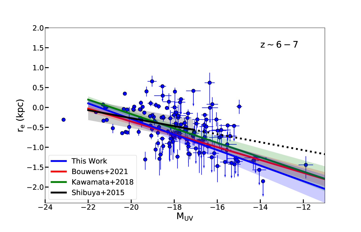
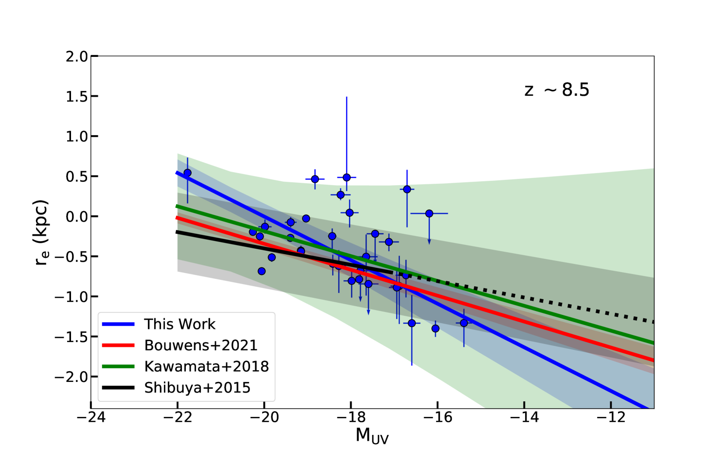
Figure 1: Intrinsic size-luminosity distribution of galaxies lensed by the six HFF clusters at z $\sim 6-7$ (top) and z$\sim$8 (bottom). The blue points represent measurements from this work, see details in Table 2 and Table 3, adopting the Bradac lens model. The solid lines in each panel represent the best-fits of the size-luminosity relation obtained by this work (blue), two other consistent results derived from lensed galaxies Bouwens et al. (2021) (red) and Kawamata et al. (2018) (green), and result derived from the blank field Shibuya et al. (2015) (black), respectively. The shadow regions show the 1$\sigma$ distribution of those. The fitting results are shown in Table 1.

Table 1: Best-fits parameters of size-luminosity distribution at z $\sim 6-7$ and z $\sim 8.5$ for five lens models.

Lens model	lg$r_{0}$	$\sigma$	$\beta$
z $\sim 6-7$
Bradac	-0.16 $\pm$ 0.11	1.33 $\pm$ 0.08	0.48 $\pm$ 0.08
Williams	-0.13 $\pm$ 0.1	1.34 $\pm$ 0.08	0.49 $\pm$ 0.08
CATs	0.00 $\pm$ 0.08	1.21 $\pm$ 0.07	0.62 $\pm$ 0.08
Zitrin	-0.05 $\pm$ 0.09	1.03 $\pm$ 0.06	0.47 $\pm$ 0.06
Sharon	-0.07 $\pm$ 0.1	1.18 $\pm$ 0.07	0.50 $\pm$ 0.07
z $\sim 8.5$
Bradac	0.21 $\pm$ 0.17	1.02 $\pm$ 0.13	0.68 $\pm$ 0.14
Williams	0.16 $\pm$ 0.18	1.44 $\pm$ 0.19	0.73 $\pm$ 0.16
CATs	0.12 $\pm$ 0.13	1.21 $\pm$ 0.16	0.78 $\pm$ 0.15
Zitrin	0.17 $\pm$ 0.19	1.27 $\pm$ 0.17	0.64 $\pm$ 0.13
Sharon	0.12 $\pm$ 0.17	1.06 $\pm$ 0.14	0.58 $\pm$ 0.14

4 Size-Luminosity distribution

The observed size-luminosity distributions of galaxies lensed by HFF clusters at z $\sim 6-7$ and z $\sim 8.5$ are shown in Figure 1. The x-axis represents the corrected UV magnitude from the ASTRODEEP catalogues, and the y-axis shows the intrinsic size measured by Lenstruction. Visually, we can tell that the more luminous galaxies tend to have a larger size. Lensing provides the ability to observe very faint and small galaxies. The faint magnitude limit reaches $\sim$-13 and the resolvable size reaches tens of pc, similar to the limits limits reported by Kawamata et al. (2018).

We present our method to derive the intrinsic size-luminosity relation in Section  4.1, and we perform the incompleteness correction based on the python code GLACiAR2 (Carrasco et al., 2018; Leethochawalit et al., 2021) in Section  4.2. Finally, in Section  4.3, we present the results of the lensing and incompleteness corrected size-luminosity relation.

4.1 Analytical description

The probability density function (PDF) of the size-luminosity pair is described as (see details in Kawamata et al. (2018)),

$$\centering\begin{split}\Psi_{\text{obs}}(r_{e},M_{\text{UV}})&=\Psi_{\text{ins}}(r_{e},M_{\text{UV}};r_{0},\sigma,\beta,M^{*},\alpha)C(r_{e},M_{\text{UV}})\\ &=P(r_{e},M_{\text{UV}};r_{0},\sigma,\beta)\phi(M_{\text{UV}};M^{*},\alpha)C(r_{e},M_{\text{UV}})\\ \end{split}\@add@centering$$ (1)

where $\Psi_{\text{obs}}$ and $\Psi_{\text{ins}}$ are the observed and intrinsic PDF, respectively, and $C(r_{e},M_{\text{UV}})$ is the completeness map as a function of size and UV magnitude, $M_{\text{UV}}$, for each cluster, see details in Section 4.2. $\Psi_{\text{ins}}$ is determined jointly by the PDF of the size distribution $P(r_{e},M_{\text{UV}};r_{0},\sigma,\beta)$ and that of the luminosity $\phi(M_{\text{UV}};M^{*},\alpha)$. $P(r_{e},M_{\text{UV}};r_{0},\sigma,\beta)$ is described by a log-normal distribution

$$P(r_{e},M_{\text{UV}};r_{0},\sigma,\beta)=\frac{1}{r_{e}\sigma\sqrt{2\pi}}exp\left(-\frac{({\rm ln}r_{e}-{\rm ln}\overline{r_{e}})^{2}}{2\sigma^{2}}\right)$$

and

$$\overline{r_{e}}=r_{0}\left(\frac{L}{L_{0}}\right)^{\beta}$$

where the r₀, $\sigma$, $\beta$ and $L_{0}$ are the radius at M${}_{\text{UV}}$=-21, the variance of the log-normal distribution, the slope of the size-luminosity relation, and luminosity corresponding to M${}_{\text{UV}}$=-21, respectively.

The luminosity function is described by the Schecheter function. Since our sample is not large enough to determine the luminosity function as well as the size luminosity relation, we fix the parameters $M^{*}$ and $\alpha$ to -20.73 and -1.86 following Kawamata et al. (2018). They demonstrated that there is no significant difference in results between free or fixed parameters of the luminosity function.

4.2 Incompleteness correction

In order to obtain the intrinsic size luminosity relation we have to account for the dependency of completeness on size and luminosity. The completeness correction is computed using the software GLACiAR2 (Carrasco et al., 2018; Leethochawalit et al., 2021), which is a public python tool for simulations of source recovery and completeness in galaxy surveys. The original code GLACiAR2 did not include the effects of gravitational lensing, therefore we modified it in order to apply it to the lensing fields.

The modified code performs the following steps to obtain the 2D completeness map $C(r_{e},M_{\text{UV}})$, where the main concept is to calculate the fraction of simulated lensed galaxies that are detected and pass the selection criteria of ASTRODEEP catalogues.

1. We select random positions uniformly on the source plane. The allowable position area in the source plane is reconstructed from mapping the image plane back to the source plane with the deflection map provided by each lens model team.

2. At each randomly selected position, we generate artificial galaxies with a range of sizes and magnitude. We set 7 bins in radius within the range $r_{e}\sim 0.1-10$ kpc, and 7 magnitude bins $M_{\text{UV}}$ from -22 to -16. Taking the lensing and PSF effects into account, we simulate how the galaxies would then appear in the F160W selection image used for catalog construction. The artificial galaxies are modeled with a Sérsic profile, with the amplitude, effective radius $r_{e}$ given by input, and index $n_{\text{S\'{e}rsic}}$ range 1-4.

3. The code runs SExtractor on the simulated image and calculates the fraction of artificial galaxies that are detected using same configuration as ASTRODEEP, i.e, HOT+COLD mode.

4. We loop through the input size and luminosity bins to derive the completeness map as a function of input size and UV magnitude.

5. We run the modified GLACiAR2 for each cluster field adopting all the available lens models at $z\sim 6-7$ and $z\sim 8.5$.

As an example, the completeness maps for the cluster Abell 2744 for five lens models and $z\sim 6-7$ are shown in Figure 5. As expected completeness decreases with decreasing luminosity and increasing size.

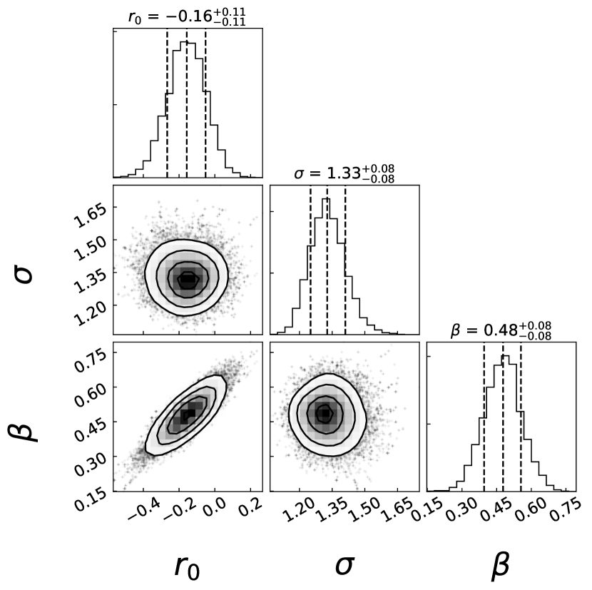
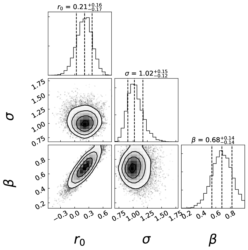
Figure 2: Posterior distribution of the r₀, $\sigma$ and $\beta$ parameters of the size-luminosity distribution at $z\sim 6-7$ (left) and $z\sim 8.5$ (right), adopting the Bradac lens model. The vertical lines in each panel display the best-fit value and 1$\sigma$ error.

4.3 Intrinsic size-luminosity relation

We use a standard Bayesian approach to derive the posterior distribution of the parameters describing the size-luminosity relation, r₀, $\sigma$, $\beta$, see Equation 1. We assume a flat prior for those three parameters. The best-fit results are shown in Figure 1, and the MCMC results of those three parameters at $z\sim 6-7$ and $z\sim 8.5$ are shown in Figure 2. Details are given in Table 1.

In Figure 1 the solid lines and shaded region represent the best-fits and 1$\sigma$ error result of size-luminosity relation at $z\sim 6-7$ (left panel) and $z\sim 8.5$ (right panel), adopting the Bradac lens model as an example. At $z\sim 6-7$, the best-fit slope $\beta$ of $r_{e}\propto L^{\beta}$ is $0.48\pm 0.08$ for the Bradac model. We derive the size-luminosity relation using all five lens models, and the results are robust with respect to the choice of lens model as detailed in Section 5. The size at $M_{\text{UV}}=-21$ is $0.69\pm 0.18$ kpc, and the variance of log-normal distribution $\sigma$ is $\sim 1.33\pm 0.08$.

At $z\sim 8.5$, the best-fit slope $\beta\sim 0.68\pm 0.14$ for the Bradac model, which is consistent with that found at $z\sim 6-7$. We also find excellent agreement between lens models as demonstrated in Figure 6. The 1$\sigma$ error is quite large, limited by sample size. We only have a handful of galaxies with reliable size measurement in this redshift range, especially at the faint end, i.e., $M_{\text{UV}}>-16$. The modal size is $1.62\pm 0.65$ kpc. The best-fit values of the intrinsic scatter $\sigma$ in two redshift ranges are similar, and also in good agreement with values determined by previous studies (Kawamata et al., 2018).

5 Comparison between lens models

In this section, we compare the results derived from different lens models, in terms of magnification, size, and completeness map as shown in Figure 3, Figure 4 and Figure 5, respectively. Taking all factors into consideration, the comparison of the best-fits results of the size-luminosity distribution is presented in Figure 6.

The magnifications derived from five lens models are shown in Figure 3. We show the distribution of the square root of the magnification $\sqrt{\mu}$, which is proportional to the source stretch scale. We characterize the distributions of the $\sqrt{\mu}$ by their median and of their 16th and 84th percentiles, p16 and p84. At $z\sim 6-7$ The mean $\sqrt{\mu}$ values of 3/5 models peak around $\sim 1.8$, while 2/5 models peak $\sim 1$. The behavior is similar at $z\sim 8.5$.

The reconstructed size distributions for each of the five lens models are shown in panels of Figure 4, and we characterize the distributions in the same manner as Figure 3. At $z\sim 6-7$, the median $r_{\text{e}}$ values is around $\sim 300-600$ pc. The median value of CATs is relatively larger, 543 pc, and the p16 value of CATs is 185 pc almost two times of other lens models, which are the results of the small median $\sqrt{\mu}$. We note that although Williams’s model has a similar median value of $\sqrt{\mu}$ and $r_{\text{e}}$ as CATs, the p16 value is at the same level as the other three lens models, bacause the size stretch factor is also affected by the shear parameters (Bouwens et al., 2021).

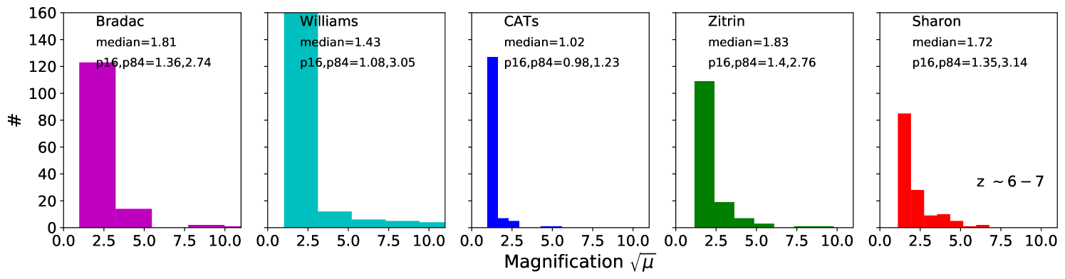
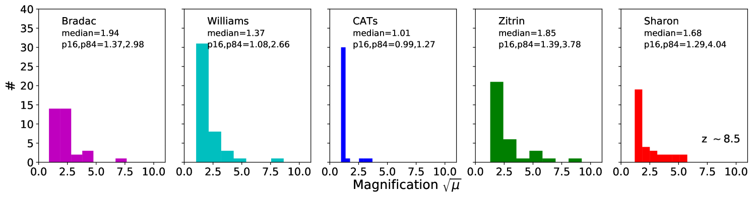
Figure 3: Comparison of the square root of magnification $\sqrt{\mu}$ between the five lens models at $z\sim 6-7$ (upper) and $z\sim 8.5$ (bottom). In each panel, we indicate the lens model, median value, and the 16th and 84th percentiles of the distribution.

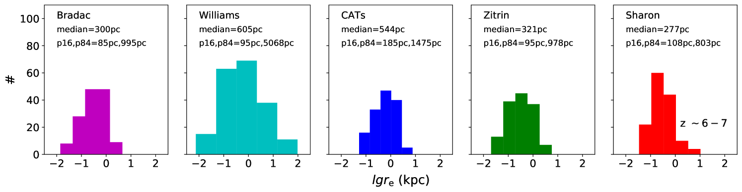
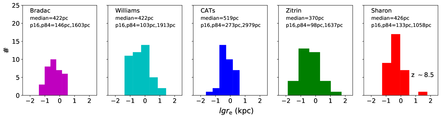
Figure 4: Comparison of reconstructed sizes $r_{\text{e}}$ between five lens models at $z\sim 6-7$ (upper) and $z\sim 8.5$ (bottom). In each panel, we indicate the lens model, median value, and the 16th and 84th percentiles of the distribution.

The completeness map is computed for each cluster using each of the five lens models. As an example, cluster A2744 is shown in Figure 5. After applying the completeness correction, we compare the inferred size-luminosity relation in Figure 6. The solids lines and shaded regions represent the best-fits and 1$\sigma$ error from each of the five lens models. The numerical results from the fits are listed in Table1. The background grey points are reconstructed from the Bradac model as a reference. As shown in Table1, the slopes based on the five lens modes are consistent with each other. We conclude that although there are discrepancies for individual sources, the inference of the size-luminosity relation is robust.

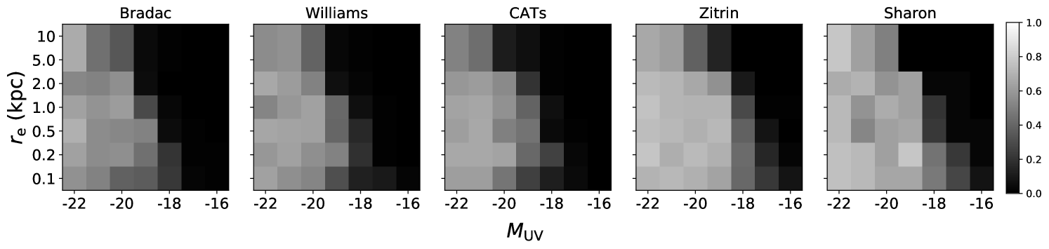
Figure 5: Completeness map of cluster A2744 for the five lens models at $z\sim 6-7$. The detection fraction is a function of UV magnitude and size. The color scheme represents the recovery fraction, darker colors corresponding to lower recovery fraction.

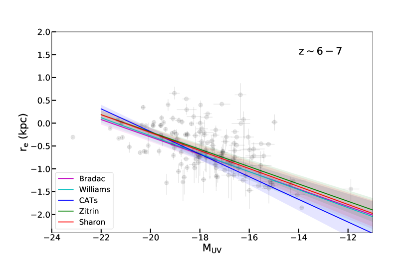
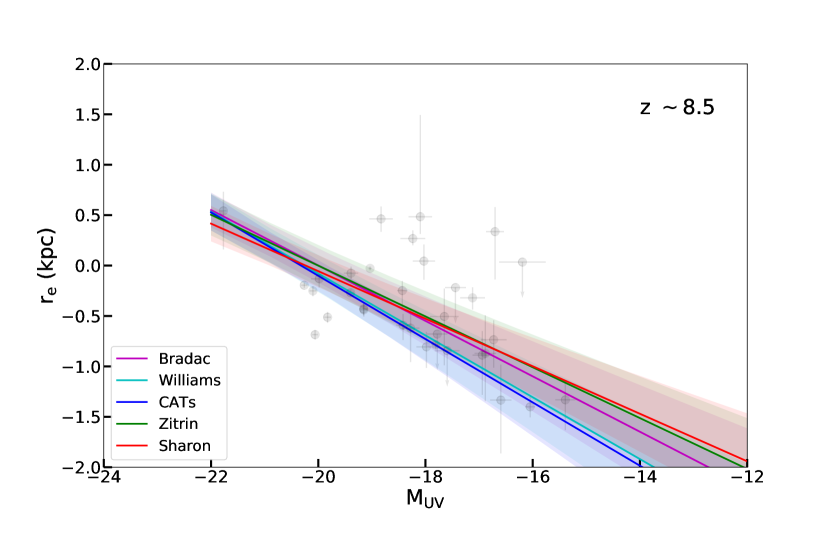
Figure 6: Comparison of the size-luminosity relations based on the different lens models. The background grey points are the measurements from the Bradac lens model, same as Figure 1. The solid lines and shaded areas indicate the best-fit and 1$\sigma$ error of size-luminosity relation. The colors represent different lens models as labeled.

6 Discussion

In this section, we first compare our results with previous work, and we then discuss the implications for the luminosity function.

6.1 Comparison with previous works

We have shown that the inferred size luminosity relation is robust with respect to the choice of lens model. We now compare our results with those obtained by other groups in blank and lensed fields. In Figure 1, the solid lines represent the results obtained by us (blue), by Bouwens et al. (2021) (red), Kawamata et al. (2018) (green) and Shibuya et al. (2015) (black), respectively. In blank fields, Shibuya et al. (2015) investigated $\sim 190,000$ HST galaxies with M${}_{\text{UV}}<-18$ and found a shallow slope of the size-luminosity relation with a constant slope $\beta=0.27\pm 0.01$ at $0<z<8$. This result is consistent with those of other studies in blank fields (e.g., Huang et al., 2013).

In contrast, in this work, we find a steeper slope $\beta\sim 0.48\pm 0.08$ and $\beta\sim 0.68\pm 0.14$ at $z\sim 6-7$ and $z\sim 8.5$ (with Bradac lens model). These finding are consistent with those of previous studies in lensed fields. Kawamata et al. (2018) used lensed galaxies in both the central and parallel fields of the six HFF clusters. They find that the slope at $z\sim 6-7$ is steep, i.e., $\beta\sim 0.46\pm 0.09$, confirming their previous result based on a smaller sample size Kawamata et al. (2015). The slope does not vary significantly in the redshift range $z\sim 6-9$, although the 1$\sigma$ errors at z$>7$ are larger due to the smaller sample size. Very recently, an independent study (Bouwens et al., 2021) revisited the relation using a similar dataset and confirmed the steepness of the slope $\beta$. They find $\beta\sim 0.40\pm 0.04$ at $z\sim 6-8$.

The difference between blank and lens fields is due to a combination of two factors. First, the lensed fields reach intrinsically fainter galaxies. Second, it is likely that the smallest galaxies are missed, or their sizes overestimated, in the blank fields.

6.2 Implication for the faint-end slope of the luminosity function

The intrinsic distribution of galaxy sizes is a crucial ingredient to determine the faint-end slope of the luminosity function, because of the effect of size on incompleteness correction, see Figure 5. In general, the smaller the galaxies, the smaller will be the completeness correction at the faint end and thus the shallower the inferred faint-end slope of the luminosity function. In turn, a shallower faint end slope will result in fewer UV photons down to a given absolute magnitude and thus require a higher escape fraction from a fainter minimum luminosity of galaxies to ionize the intergalactic medium. Of course, there are other factors to be taken into account. For example, photons might escape more easily from a very compact source, thus somewhat compensating the smaller numbers via a higher escape fraction.

In conclusion, our work confirms the steep slope of the size luminosity relation found by Bouwens et al. (2021) and Kawamata et al. (2018), demonstrating that the result is robust to the choice of lens model and it is thus not driven by lens mode uncertainties.

7 Conclusion

In this paper, we revisited the size-luminosity relation of galaxies at the epoch of reionization. We focused on the six HFF cluster fields and compared the performance of five publicly available lens models. Our sample is selected from the multi-wavelength photometric catalogue made by the ASTRODEEP group, size measurements are conducted via the modified Lenstruction software and we correct for observational incompleteness via the GLACiAR2 software. We summarize our results as follows,

1. Parametrizing the size-luminosity relation as $r_{e}\propto L^{\beta}$, we find a slope $\beta\sim 0.48\pm 0.08$ at $z\sim 6-7$ and $\beta\sim 0.68\pm 0.14$ at $z\sim 8.5$, adopting the Bradac lens model. The slope is steeper than that found in blank fields and consistent with that found by previous studies in lensing fields.

2. The slope $\beta$ is robust with respect to the choice of lens model and varies by less than the reported uncertainties.

Our study demonstrates that the steeper slope found in lensing fields with respect to blank fields cannot be explained with lens modeling systematics. We attribute the steeper slope to the fainter luminosity and higher angular resolution achieved in lensing fields, which allows us to measure intrinsically smaller galaxy sizes at the faint end.

The steep slope of the size luminosity relation has implications for cosmic reionization as incompleteness depends on intrinsic galaxy size. Therefore, qualitatively, a steep slope of the size luminosity relation will result in a shallower faint end slope of the galaxy luminosity function. Studies with larger samples of lensed galaxies are needed to fully quantify this effect.

The successful launch of the James Webb Space Telescope and the data taken under programs such as ERS-1324 will allow us to carry out such studies, by probing even fainter magnitudes and smaller sizes, and simultaneously constrain the size luminosity relation and the galaxy luminosity function.

Table 2: Fitting results for galaxies lensed by six HFF clusters at $z\sim 6-7$, adopting the Bradac lens model. From left to right, the columns represent the ID in the ASTRODEEP catalogue of source, RA and Dec of the center of light, photometric redshift, circularized effective radius $r_{e}$, and UV magnitude.

ID	RA	Dec	z${}_{\text{photo}}$	re/kpc	M${}_{\text{UV}}$
Abell 2744
62	3.604872	-30.415848	6.13	0.91 $\pm$ 0.08	-20.35 $\pm$ 0.04
73	3.593802	-30.415447	6.85	0.13 $\pm$ 0.03	-18.75 $\pm$ 0.05
106	3.570654	-30.414661	6.04	0.20 $\pm$ 0.03	-19.07 $\pm$ 0.06
189	3.592944	-30.413328	5.68	0.11 $\pm$ 0.04	-16.44 $\pm$ 0.14
397	3.603215	-30.410353	6.31	0.24 $\pm$ 0.04	-17.08 $\pm$ 0.10
437	3.604567	-30.409365	5.87	0.09 $\pm$ 0.04	-15.56 $\pm$ 0.22
446	3.604751	-30.409292	6.02	0.36 $\pm$ 0.07	-16.61 $\pm$ 0.13
561	3.606384	-30.407278	6.37	0.06 $\pm$ 0.03	-17.85 $\pm$ 0.10
855	3.601075	-30.403990	6.02	0.33 $\pm$ 0.13	-17.48 $\pm$ 0.13
863	3.570069	-30.403721	5.87	0.25 $\pm$ 0.04	-18.29 $\pm$ 0.07
1622	3.586268	-30.392712	5.86	<0.05	-15.15 $\pm$ 0.39
1989	3.606223	-30.386644	5.59	0.35 $\pm$ 0.03	-19.10 $\pm$ 0.04
2002	3.576895	-30.386328	6.46	0.03 $\pm$ 0.02	-15.99 $\pm$ 0.16
2007	3.588642	-30.386244	5.82	0.07 $\pm$ 0.07	-16.83 $\pm$ 0.29
2202	3.603425	-30.383219	5.86	0.10 $\pm$ 0.07	-17.34 $\pm$ 0.11
2434	3.590547	-30.379766	5.82	0.39 $\pm$ 0.15	-16.97 $\pm$ 0.16
2452	3.590790	-30.379410	5.74	0.97 $\pm$ 0.10	-18.34 $\pm$ 0.09
20214	3.572779	-30.413527	5.84	0.50 $\pm$ 0.21	-16.04 $\pm$ 0.23
20295	3.591288	-30.412630	6.06	0.12 $\pm$ 0.10	-15.54 $\pm$ 0.44
20785	3.605206	-30.407106	5.85	0.19 $\pm$ 0.05	-15.41 $\pm$ 0.30
21380	3.568028	-30.401043	6.10	0.14 $\pm$ 0.10	-18.06 $\pm$ 0.22
21582	3.589428	-30.398497	5.88	0.04 $\pm$ 0.02	-11.88 $\pm$ 0.34
21690	3.572050	-30.397192	5.54	<0.35	-15.52 $\pm$ 0.40
22064	3.592817	-30.393698	5.84	<0.03	-14.05 $\pm$ 0.32
22392	3.587827	-30.390039	5.72	<0.04	-15.04 $\pm$ 0.22
22542	3.593637	-30.388189	6.05	0.04 $\pm$ 0.04	-15.34 $\pm$ 0.29
23153	3.597839	-30.381126	6.11	0.25 $\pm$ 0.12	-16.59 $\pm$ 0.26
23460	3.575475	-30.408583	6.10	0.07 $\pm$ 0.06	-16.14 $\pm$ 0.21
MACS J0416.1-2403
13	64.047569	-24.097076	5.70	0.30 $\pm$ 0.08	-20.85 $\pm$ 0.05
111	64.038246	-24.092775	6.83	0.05 $\pm$ 0.02	-19.35 $\pm$ 0.06
139	64.039261	-24.091812	6.70	1.04 $\pm$ 0.10	-19.86 $\pm$ 0.06
220	64.034561	-24.089703	5.82	0.22 $\pm$ 0.09	-17.75 $\pm$ 0.15
247	64.040497	-24.088909	7.13	0.58 $\pm$ 0.14	-18.95 $\pm$ 0.10
271	64.039551	-24.088541	5.93	0.54 $\pm$ 0.05	-19.58 $\pm$ 0.06
355	64.038498	-24.087040	6.24	0.39 $\pm$ 0.15	-17.93 $\pm$ 0.17
735	64.054390	-24.081661	6.33	1.18 $\pm$ 0.09	-21.31 $\pm$ 0.04
1827	64.050858	-24.066542	5.91	0.16 $\pm$ 0.13	-18.15 $\pm$ 0.14
1829	64.051079	-24.066517	5.96	<0.14	-16.87 $\pm$ 0.20
2179	64.047852	-24.062069	6.15	0.22 $\pm$ 0.04	-18.12 $\pm$ 0.07
2204	64.039978	-24.061810	6.30	0.41 $\pm$ 0.12	-17.52 $\pm$ 0.13
2236	64.037483	-24.061234	5.97	0.12 $\pm$ 0.06	-17.37 $\pm$ 0.13
2240	64.047150	-24.061132	5.75	0.24 $\pm$ 0.17	-17.05 $\pm$ 0.07
2324	64.044479	-24.059311	6.29	<0.34	-15.22 $\pm$ 0.25
2337	64.043571	-24.059002	6.14	<0.65	-16.58 $\pm$ 0.16
2411	64.042946	-24.057184	5.91	<0.06	-16.26 $\pm$ 0.20
20065	64.042404	-24.095959	5.80	<0.13	-16.74 $\pm$ 0.35
20103	64.042519	-24.094933	5.78	0.16 $\pm$ 0.12	-16.64 $\pm$ 0.33
20470	64.037987	-24.086891	5.87	0.18 $\pm$ 0.09	-15.89 $\pm$ 0.49
20594	64.037933	-24.085415	6.04	0.26 $\pm$ 0.15	-15.98 $\pm$ 0.41
20618	64.040710	-24.085100	5.91	0.27 $\pm$ 0.10	-15.82 $\pm$ 0.44
20722	64.022423	-24.083601	6.15	0.05 $\pm$ 0.02	-14.32 $\pm$ 0.25
20914	64.037971	-24.081451	5.87	<0.05	-14.22 $\pm$ 0.52
21216	64.020332	-24.078485	5.75	<0.19	-15.81 $\pm$ 0.35
21650	64.046074	-24.073437	6.10	<0.33	-16.51 $\pm$ 0.32
21659	64.019035	-24.073301	6.36	2.61 $\pm$ 0.64	-17.11 $\pm$ 0.34
21869	64.049286	-24.070938	6.15	0.71 $\pm$ 0.16	-17.35 $\pm$ 0.22
22453	64.050079	-24.064102	5.79	<0.04	-15.64 $\pm$ 0.23
22971	64.037361	-24.057997	5.99	0.23 $\pm$ 0.12	-17.07 $\pm$ 0.23

Table 2: (Continued)

ID	RA	Dec	z${}_{\text{photo}}$	re/kpc	M${}_{\text{UV}}$
MACS J1149.5+2223
354	177.393036	22.381325	5.66	<0.18	-18.03 $\pm$ 0.15
404	177.388382	22.382391	6.20	0.24 $\pm$ 0.05	-19.65 $\pm$ 0.08
433	177.384644	22.382761	6.16	<0.16	-18.56 $\pm$ 0.13
825	177.425262	22.386383	6.61	0.49 $\pm$ 0.01	-23.14 $\pm$ 0.01
1243	177.384537	22.392721	5.92	1.06 $\pm$ 0.15	-18.72 $\pm$ 0.11
1494	177.382538	22.395403	5.76	0.87 $\pm$ 0.05	-19.89 $\pm$ 0.05
2364	177.387711	22.405834	5.71	4.17 $\pm$ 3.14	-16.35 $\pm$ 0.23
2368	177.418457	22.405724	5.94	0.47 $\pm$ 0.14	-19.52 $\pm$ 0.07
2410	177.418625	22.406404	6.00	0.63 $\pm$ 0.09	-19.02 $\pm$ 0.10
2535	177.409424	22.408207	5.54	0.29 $\pm$ 0.05	-19.03 $\pm$ 0.07
2619	177.403015	22.409502	5.79	0.32 $\pm$ 0.06	-18.71 $\pm$ 0.07
2747	177.407974	22.411522	6.17	< 0.35	-17.92 $\pm$ 0.23
2966	177.412933	22.413643	6.40	0.07 $\pm$ 0.04	-18.64 $\pm$ 0.11
3027	177.402725	22.414614	5.83	0.18 $\pm$ 0.09	-17.74 $\pm$ 0.16
3054	177.412018	22.415779	5.79	1.03 $\pm$ 0.02	-21.14 $\pm$ 0.02
3162	177.414688	22.417059	6.07	0.55 $\pm$ 0.11	-18.51 $\pm$ 0.14
20570	177.393036	22.381321	5.75	0.18 $\pm$ 0.13	-18.00 $\pm$ 0.13
21231	177.397278	22.387806	5.85	<0.98	-16.34 $\pm$ 0.37
22626	177.386780	22.401293	5.96	<0.55	-17.39 $\pm$ 0.17
22717	177.393097	22.402140	5.80	0.16 $\pm$ 0.11	-17.41 $\pm$ 0.14
23096	177.380600	22.405464	5.64	<0.27	-17.48 $\pm$ 0.19
23485	177.403015	22.409500	5.91	0.23 $\pm$ 0.05	-18.76 $\pm$ 0.07
23874	177.412933	22.413645	6.46	0.05 $\pm$ 0.04	-18.69 $\pm$ 0.08
24039	177.412018	22.415777	5.98	1.01 $\pm$ 0.02	-21.20 $\pm$ 0.02
MACS J0717.5+3745
82	109.389275	37.724854	6.05	0.56 $\pm$ 0.05	-18.59 $\pm$ 0.08
136	109.381462	37.726364	5.58	0.90 $\pm$ 0.08	-19.90 $\pm$ 0.05
203	109.379547	37.728397	6.25	2.22 $\pm$ 0.24	-20.30 $\pm$ 0.08
208	109.378731	37.728226	6.17	4.53 $\pm$ 1.47	-19.03 $\pm$ 0.21
246	109.378822	37.729141	5.60	0.89 $\pm$ 0.10	-19.57 $\pm$ 0.11
250	109.378723	37.729404	7.20	1.39 $\pm$ 0.69	-18.25 $\pm$ 0.28
332	109.376572	37.731480	6.31	1.27 $\pm$ 0.22	-19.09 $\pm$ 0.15
336	109.381050	37.731613	6.10	<0.10	-18.21 $\pm$ 0.10
356	109.378174	37.731903	6.16	0.50 $\pm$ 0.21	-16.93 $\pm$ 0.23
374	109.377205	37.732182	6.25	0.20 $\pm$ 0.07	-18.04 $\pm$ 0.17
392	109.376816	37.732525	6.03	0.75 $\pm$ 0.18	-17.91 $\pm$ 0.24
471	109.412857	37.733803	6.53	0.05 $\pm$ 0.01	-15.10 $\pm$ 0.08
510	109.413666	37.734642	6.46	<0.01	-13.87 $\pm$ 0.08
640	109.376984	37.736454	6.02	0.58 $\pm$ 0.07	-18.51 $\pm$ 0.09
774	109.379036	37.738388	5.93	0.18 $\pm$ 0.09	-16.59 $\pm$ 0.16
797	109.391907	37.737995	5.97	2.49 $\pm$ 1.08	-17.97 $\pm$ 0.04
813	109.418655	37.738789	5.90	<0.07	-16.62 $\pm$ 0.18
1095	109.377609	37.741798	5.73	0.19 $\pm$ 0.06	-17.12 $\pm$ 0.11
1202	109.390739	37.742214	6.13	0.88 $\pm$ 0.04	-20.19 $\pm$ 0.03
1737	109.408783	37.748375	6.04	1.05 $\pm$ 0.43	-14.98 $\pm$ 0.13
1841	109.380402	37.749458	5.74	0.26 $\pm$ 0.07	-17.76 $\pm$ 0.13
2090	109.386215	37.751919	6.31	1.03 $\pm$ 0.09	-19.47 $\pm$ 0.06
2169	109.384567	37.753006	5.86	0.49 $\pm$ 0.04	-21.14 $\pm$ 0.02
2312	109.409065	37.754684	6.12	0.11 $\pm$ 0.02	-18.51 $\pm$ 0.05
2368	109.412941	37.755592	5.75	1.15 $\pm$ 0.17	-18.85 $\pm$ 0.16
2883	109.399109	37.764957	6.37	0.74 $\pm$ 0.08	-19.39 $\pm$ 0.06
20950	109.370537	37.738941	5.59	1.20 $\pm$ 0.85	-16.23 $\pm$ 0.26
23199	109.403320	37.765663	5.88	0.14 $\pm$ 0.18	-16.73 $\pm$ 0.23
23588	109.385132	37.758907	6.08	0.04 $\pm$ 0.02	-15.20 $\pm$ 0.29

Table 2: (Continued)

ID	RA	Dec	z${}_{\text{photo}}$	re/kpc	M${}_{\text{UV}}$
Abell S1063
165	342.201924	-44.549906	5.93	2.53 $\pm$ 0.73	-19.29 $\pm$ 0.08
242	342.194600	-44.548404	5.83	3.40 $\pm$ 3.27	-18.55 $\pm$ 0.17
247	342.177057	-44.548331	6.16	1.30 $\pm$ 0.19	-19.55 $\pm$ 0.09
325	342.177695	-44.546933	6.28	0.90 $\pm$ 0.11	-19.59 $\pm$ 0.05
438	342.173075	-44.545251	6.29	0.53 $\pm$ 0.29	-18.18 $\pm$ 0.13
617	342.193776	-44.542721	6.44	<0.37	-17.69 $\pm$ 0.19
626	342.176131	-44.542668	6.21	0.23 $\pm$ 0.05	-17.92 $\pm$ 0.08
652	342.167993	-44.542512	6.04	0.07 $\pm$ 0.02	-17.28 $\pm$ 0.04
1033	342.190892	-44.537462	6.11	0.23 $\pm$ 0.01	-20.42 $\pm$ 0.02
1142	342.198542	-44.535311	5.52	<0.50	-16.51 $\pm$ 0.22
1143	342.183924	-44.535317	6.11	0.20 $\pm$ 0.10	-17.13 $\pm$ 0.21
1233	342.181055	-44.534609	6.11	0.46 $\pm$ 0.02	-21.29 $\pm$ 0.03
1690	342.164364	-44.530232	6.12	0.65 $\pm$ 0.16	-18.00 $\pm$ 0.11
1717	342.189053	-44.530028	6.11	0.77 $\pm$ 0.02	-21.64 $\pm$ 0.03
2073	342.173329	-44.525929	5.91	0.07 $\pm$ 0.03	-17.34 $\pm$ 0.07
2592	342.171298	-44.519801	6.11	0.32 $\pm$ 0.41	-20.09 $\pm$ 0.03
2608	342.172002	-44.519331	6.55	0.55 $\pm$ 0.39	-17.82 $\pm$ 0.17
2932	342.169900	-44.515155	6.74	<1.35	-17.73 $\pm$ 0.24
2955	342.165543	-44.514668	6.14	1.61 $\pm$ 1.04	-17.68 $\pm$ 0.17
3001	342.173965	-44.514089	5.98	1.00 $\pm$ 0.43	-17.98 $\pm$ 0.18
Abell 370
729	39.968278	-1.597248	6.80	<0.62	-17.82 $\pm$ 0.38
2026	39.985087	-1.578782	6.75	1.97 $\pm$ 0.56	-18.53 $\pm$ 0.40
2356	39.986285	-1.575199	5.62	0.12 $\pm$ 0.09	-18.23 $\pm$ 0.21
2843	39.985811	-1.571304	6.32	0.45 $\pm$ 0.10	-18.92 $\pm$ 0.16
3238	39.982590	-1.566664	6.65	<0.09	-16.99 $\pm$ 0.27
3241	39.980269	-1.566761	6.17	0.09 $\pm$ 0.04	-18.86 $\pm$ 0.09
3252	39.980109	-1.566731	6.10	0.60 $\pm$ 0.08	-19.12 $\pm$ 0.10
3822	39.978189	-1.558981	6.77	0.24 $\pm$ 0.03	-20.26 $\pm$ 0.04
3825	39.978067	-1.558955	6.77	0.23 $\pm$ 0.02	-20.18 $\pm$ 0.04

Table 3: Same as Table 2, for galaxies at $z\sim 8.5$.

ID	RA	Dec	z${}_{\text{photo}}$	re/kpc	M${}_{\text{UV}}$
Abell 2744
409	3.592160	-30.409914	7.66	<0.16	-16.56 $\pm$ 0.19
548	3.576798	-30.407442	8.56	0.31 $\pm$ 0.13	-17.77 $\pm$ 0.20
2036	3.596087	-30.385836	8.32	0.36 $\pm$ 0.04	-19.37 $\pm$ 0.07
2248	3.603863	-30.382261	8.02	0.50 $\pm$ 0.07	-20.04 $\pm$ 0.07
2257	3.598123	-30.382393	7.53	0.34 $\pm$ 0.15	-17.74 $\pm$ 0.18
2261	3.603996	-30.382309	7.97	1.07 $\pm$ 0.18	-19.32 $\pm$ 0.10
2264	3.603382	-30.382252	8.29	0.94 $\pm$ 0.04	-20.29 $\pm$ 0.06
2316	3.605061	-30.381470	7.66	0.52 $\pm$ 0.18	-18.60 $\pm$ 0.19
2346	3.606460	-30.380995	7.79	0.45 $\pm$ 0.08	-19.86 $\pm$ 0.06
2365	3.604516	-30.380468	8.20	0.35 $\pm$ 0.03	-20.84 $\pm$ 0.05
20236	3.572523	-30.413267	8.46	1.03 $\pm$ 0.21	-18.01 $\pm$ 0.24
21573	3.579663	-30.398682	7.75	0.05 $\pm$ 0.03	-15.57 $\pm$ 0.19
22347	3.588001	-30.390648	8.80	0.12 $\pm$ 0.07	-16.62 $\pm$ 0.20
MACS J0416.1-2403
99	64.039162	-24.093182	8.66	0.76 $\pm$ 0.04	-20.54 $\pm$ 0.05
218	64.027420	-24.089979	7.68	1.26 $\pm$ 0.04	-19.83 $\pm$ 0.03
286	64.037567	-24.088116	8.14	0.24 $\pm$ 0.10	-18.22 $\pm$ 0.17
726	64.047981	-24.081671	8.32	0.29 $\pm$ 0.03	-19.94 $\pm$ 0.06
743	64.048058	-24.081427	8.94	0.61 $\pm$ 0.07	-20.24 $\pm$ 0.06
1253	64.019333	-24.075153	7.66	2.65 $\pm$ 0.50	-18.79 $\pm$ 0.22
1997	64.049583	-24.064596	8.10	0.15 $\pm$ 0.05	-17.82 $\pm$ 0.17
20465	64.049088	-24.086967	7.53	2.54 $\pm$ 0.73	-18.96 $\pm$ 0.22
21169	64.041405	-24.078926	8.03	<0.11	-17.11 $\pm$ 0.23
21864	64.024414	-24.070963	7.64	1.12 $\pm$ 0.44	-18.52 $\pm$ 0.21
21997	64.039139	-24.069435	7.95	0.25 $\pm$ 0.06	-15.71 $\pm$ 0.23
22035	64.038971	-24.069519	7.65	0.62 $\pm$ 0.08	-18.56 $\pm$ 0.14
22746	64.046509	-24.061630	8.36	0.40 $\pm$ 0.20	-17.27 $\pm$ 0.23
MACS J1149.5+2223
2316	177.407684	22.405251	7.93	<0.22	-16.91 $\pm$ 0.27
22863	177.388184	22.403442	7.66	<0.70	-14.83 $\pm$ 0.43
MACS J0717.5+3745
23536	109.400124	37.746799	8.45	0.51 $\pm$ 0.67	-17.90 $\pm$ 0.06
Abell S1063
2048	342.182253	-44.526073	8.81	0.10 $\pm$ 0.02	-16.40 $\pm$ 0.13
2086	342.179829	-44.525664	8.85	0.13 $\pm$ 0.02	-16.67 $\pm$ 0.09
Abell 370
849	39.966126	-1.594771	7.70	0.07 $\pm$ 0.03	-16.68 $\pm$ 0.19
2867	39.992152	-1.570892	8.20	0.57 $\pm$ 0.13	-19.51 $\pm$ 0.15

Data Availability

The SEDs, cutouts, and all ancillary information of galaxies used in this article can be found on the ASTRODEEP CDS Interface at http://www.astrodeep.eu/cds-interface/.

References

- Birrer & Amara (2018) Birrer S., Amara A., 2018, Physics of the Dark Universe, 22, 189
- Birrer et al. (2015) Birrer S., Amara A., Refregier A., 2015, ApJ, 813, 102
- Birrer et al. (2021) Birrer S., et al., 2021, The Journal of Open Source Software, 6, 3283
- Bouwens et al. (2017) Bouwens R. J., Illingworth G. D., Oesch P. A., Atek H., Lam D., Stefanon M., 2017, ApJ, 843, 41
- Bouwens et al. (2021) Bouwens R. J., Illingworth G. D., van Dokkum P. G., Oesch P. A., Stefanon M., Ribeiro B., 2021, arXiv e-prints, p. arXiv:2112.02948
- Bradač et al. (2005) Bradač M., Schneider P., Lombardi M., Erben T., 2005, A&A, 437, 39
- Bradač et al. (2009) Bradač M., et al., 2009, ApJ, 706, 1201
- Bradač et al. (2019) Bradač M., et al., 2019, MNRAS, 489, 99
- Carollo et al. (2013) Carollo C. M., et al., 2013, ApJ, 773, 112
- Carrasco et al. (2018) Carrasco D., Trenti M., Mutch S., Oesch P. A., 2018, Publ. Astron. Soc. Australia, 35, e022
- Castellano et al. (2016) Castellano M., et al., 2016, A&A, 590, A31
- Choi et al. (2018) Choi E., Somerville R. S., Ostriker J. P., Naab T., Hirschmann M., 2018, ApJ, 866, 91
- Coe et al. (2015) Coe D., Bradley L., Zitrin A., 2015, ApJ, 800, 84
- Di Criscienzo et al. (2017) Di Criscienzo M., et al., 2017, A&A, 607, A30
- Dutton et al. (2007) Dutton A. A., van den Bosch F. C., Dekel A., Courteau S., 2007, ApJ, 654, 27
- Fall & Efstathiou (1980) Fall S. M., Efstathiou G., 1980, MNRAS, 193, 189
- Fan et al. (2006) Fan X., et al., 2006, AJ, 132, 117
- Foreman-Mackey et al. (2013) Foreman-Mackey D., Hogg D. W., Lang D., Goodman J., 2013, PASP, 125, 306
- Grazian et al. (2011) Grazian A., et al., 2011, A&A, 532, A33
- Grazian et al. (2012) Grazian A., et al., 2012, A&A, 547, A51
- Grillo et al. (2015) Grillo C., et al., 2015, ApJ, 800, 38
- Hoag et al. (2016) Hoag A., et al., 2016, The Astrophysical Journal, 831, 182
- Huang et al. (2013) Huang K.-H., Ferguson H. C., Ravindranath S., Su J., 2013, ApJ, 765, 68
- Ishigaki et al. (2015) Ishigaki M., Kawamata R., Ouchi M., Oguri M., Shimasaku K., Ono Y., 2015, ApJ, 799, 12
- Jauzac et al. (2012) Jauzac M., et al., 2012, MNRAS, 426, 3369
- Jauzac et al. (2014) Jauzac M., et al., 2014, MNRAS, 443, 1549
- Johnson et al. (2014) Johnson T. L., Sharon K., Bayliss M. B., Gladders M. D., Coe D., Ebeling H., 2014, ApJ, 797, 48
- Jullo & Kneib (2009) Jullo E., Kneib J. P., 2009, MNRAS, 395, 1319
- Jullo et al. (2007) Jullo E., Kneib J. P., Limousin M., Elíasdóttir Á., Marshall P. J., Verdugo T., 2007, New Journal of Physics, 9, 447
- Kawamata et al. (2015) Kawamata R., Ishigaki M., Shimasaku K., Oguri M., Ouchi M., 2015, ApJ, 804, 103
- Kawamata et al. (2018) Kawamata R., Ishigaki M., Shimasaku K., Oguri M., Ouchi M., Tanigawa S., 2018, ApJ, 855, 4
- Kawinwanichakij et al. (2021) Kawinwanichakij L., et al., 2021, ApJ, 921, 38
- Laporte et al. (2016) Laporte N., et al., 2016, ApJ, 820, 98
- Leethochawalit et al. (2021) Leethochawalit N., Trenti M., Morishita T., Roberts-Borsani G., Treu T., 2021, MNRAS,
- Liesenborgs et al. (2006) Liesenborgs J., De Rijcke S., Dejonghe H., 2006, MNRAS, 367, 1209
- López-Sanjuan et al. (2012) López-Sanjuan C., et al., 2012, A&A, 548, A7
- Lotz et al. (2017) Lotz J. M., et al., 2017, ApJ, 837, 97
- Mason et al. (2018) Mason C. A., Treu T., Dijkstra M., Mesinger A., Trenti M., Pentericci L., de Barros S., Vanzella E., 2018, ApJ, 856, 2
- Meneghetti et al. (2017) Meneghetti M., et al., 2017, MNRAS, 472, 3177
- Merlin et al. (2015) Merlin E., et al., 2015, A&A, 582, A15
- Merlin et al. (2016) Merlin E., et al., 2016, A&A, 590, A30
- Merten et al. (2009) Merten J., Cacciato M., Meneghetti M., Mignone C., Bartelmann M., 2009, A&A, 500, 681
- Merten et al. (2011) Merten J., et al., 2011, MNRAS, 417, 333
- Mo et al. (1998) Mo H. J., Mao S., White S. D. M., 1998, MNRAS, 295, 319
- Mohammed et al. (2014) Mohammed I., Liesenborgs J., Saha P., Williams L. L. R., 2014, MNRAS, 439, 2651
- Mosleh et al. (2012) Mosleh M., et al., 2012, ApJ, 756, L12
- Mosleh et al. (2017) Mosleh M., Tacchella S., Renzini A., Carollo C. M., Molaeinezhad A., Onodera M., Khosroshahi H. G., Lilly S., 2017, ApJ, 837, 2
- Mowla et al. (2019) Mowla L. A., et al., 2019, ApJ, 880, 57
- Neufeld et al. (2021) Neufeld C., et al., 2021, arXiv e-prints, p. arXiv:2111.14882
- Oesch et al. (2010) Oesch P. A., et al., 2010, ApJ, 709, L21
- Paulino-Afonso et al. (2018) Paulino-Afonso A., et al., 2018, MNRAS, 476, 5479
- Peng et al. (2002) Peng C. Y., Ho L. C., Impey C. D., Rix H.-W., 2002, AJ, 124, 266
- Richard et al. (2014) Richard J., et al., 2014, MNRAS, 444, 268
- Scannapieco et al. (2008) Scannapieco C., Tissera P. B., White S. D. M., Springel V., 2008, MNRAS, 389, 1137
- Shen et al. (2003) Shen S., Mo H. J., White S. D. M., Blanton M. R., Kauffmann G., Voges W., Brinkmann J., Csabai I., 2003, MNRAS, 343, 978
- Shibuya et al. (2015) Shibuya T., Ouchi M., Harikane Y., 2015, ApJS, 219, 15
- Shipley et al. (2018) Shipley H. V., et al., 2018, ApJS, 235, 14
- Tacconi et al. (2008) Tacconi L. J., et al., 2008, ApJ, 680, 246
- Trujillo et al. (2006) Trujillo I., et al., 2006, ApJ, 650, 18
- Vanzella et al. (2021) Vanzella E., et al., 2021, A&A, 646, A57
- Wechsler & Tinker (2018) Wechsler R. H., Tinker J. L., 2018, ARA&A, 56, 435
- Wellons et al. (2016) Wellons S., et al., 2016, MNRAS, 456, 1030
- Whitaker et al. (2017) Whitaker K. E., et al., 2017, ApJ, 838, 19
- Williams et al. (2010) Williams R. J., Quadri R. F., Franx M., van Dokkum P., Toft S., Kriek M., Labbé I., 2010, ApJ, 713, 738
- Yang et al. (2020) Yang L., Birrer S., Treu T., 2020, MNRAS, 496, 2648
- Yang et al. (2021) Yang L., Roberts-Borsani G., Treu T., Birrer S., Morishita T., Bradač M., 2021, MNRAS, 501, 1028
- Yue et al. (2018) Yue B., et al., 2018, ApJ, 868, 115
- Zitrin et al. (2009) Zitrin A., et al., 2009, MNRAS, 396, 1985
- Zitrin et al. (2013) Zitrin A., et al., 2013, ApJ, 762, L30
- van Dokkum et al. (2008) van Dokkum P. G., et al., 2008, ApJ, 677, L5
- van der Wel et al. (2014) van der Wel A., et al., 2014, ApJ, 788, 28