Controlling extrapolations of nuclear properties with feature selection
Abstract
Predictions of nuclear properties far from measured data are inherently imprecise because of uncertainties in our knowledge of nuclear forces and in our treatment of quantum many-body effects in strongly-interacting systems. While the model bias can be directly calculated when experimental data is available, only an estimate can be made in the absence of such measurements. Current approaches to compute the estimated bias quickly lose predictive power when input variables such as proton or neutron number are extrapolated, resulting in uncontrolled uncertainties in applications such as nucleosynthesis simulations. In this letter, we present a novel technique to identify the input variables of machine learning algorithms that can provide robust estimates of model bias. Our process is based on selecting input variables, or features, based on their probability distribution functions across the entire nuclear chart. We illustrate our approach on the problem of quantifying the model bias in nuclear binding energies calculated with Density Functional Theory (DFT). We show that feature selection can systematically improve theoretical predictions without increasing uncertainties.
Introduction - Nuclear physics models are at the heart of some of the most important contemporary scientific problems. Prominent examples include probing the limits of the periodic table of elements [1], understanding the mechanisms of nuclear fission for basic science and carbon-free energy production sources [2] or simulating the formation of elements in the universe through a set of nuclear reactions in various stellar environments [3]. These problems require a complete description of nuclear properties for all nuclei across the nuclear chart, but only a very small subset of them have been measured experimentally. With the coming online of next-generation radioactive ion beam facilities, many of the gaps in our knowledge will be filled [4]. Yet, the vast majority of nuclear data will remain out of reach and will have to be determined through theoretical simulations.
Atomic nuclei are self-bound, strongly-interacting quantum many-body systems [5, 6]. The nuclear forces that bind them are not elementary interactions but are derived from non-perturbative quantum chromodynamics [7, 8, 9]. For these reasons, an exact description of the nucleus is impossible and approximations are needed [10, 11, 12, 13, 14]. As a result, all theories of the nucleus are in fact models characterized, among others, by a small number of parameters that must be calibrated to experimental data. Most importantly, the accuracy and precision of nuclear models tend to be far lower than what direct experimental measurements can deliver. For example, state-of-the-art mass models predict nuclear binding energies to within about 500 keV [15, 16] while Penning-trap mass measurements yield results within a few eV – about 500 000 times more precise [17, 18]. In other words, nuclear models are inherently imperfect. Extrapolations far from the calibration region with such models are bound to come with a potentially very large bias.
The problems of calibrating nuclear model parameters, of quantifying and propagating the related uncertainties, and of estimating prediction biases have spurred interest in machine learning (ML) algorithms [19, 20, 21, 22, 23, 24, 25, 26, 27, 28, 29]. These new applications have resulted in better estimates for the limits of the nuclear chart [30], improved mass tables [20, 21, 22], and extrapolations of no-core shell model ground-state energies and radii to very large model spaces [25]. A recent workshop on “AI for nuclear physics” presented an in-depth report of current and possible applications of the broader field of artificial intelligence (AI) to nuclear physics [31]. While AI/ML techniques have been used to correct imperfect nuclear models, the reliability of the resulting predictions far outside the range of measured data has been seldom addressed.
The usual approach in AI/ML starts by defining a specific relationship, represented as an algorithm, between a set of input variables (features) and a set of output variables (targets). This algorithm usually contains a set of adjustable parameters. Typical examples include Gaussian Processes, Support Vector Machines and Bayesian Neural Networks. The training of the algorithm is nothing but the determination of its parameters by minimizing the distance between the algorithm’s output for a set of features-targets pairs and the physical world observations. In its most fundamental sense, this is similar to using an interpolating polynomial to reproduce a set of given points.
Similar to polynomial interpolation, machine learning training can thus result in overfitting. This can be mitigated by randomly splitting the available physical world data into training and testing sets. The algorithm is trained with a subset of all available data and its performance is tested against the remaining data. The training process is fine-tuned until the algorithm’s performance is comparable with the training and testing data. This process ensures that the algorithm will make reliable predictions with new feature values, as long as those values are within the training/testing domain (i.e. interpolating). However there is no guarantee of reliable predictions when the features are taken outside of the training/testing domain (i.e. extrapolating). This would be akin to training an image recognition software with pictures of dogs and wolfs, and then using it to identify the animals in a picture of a lake with ducks and geese. For a simple and pedagogical demonstration of the limits to extrapolations with an artificial neural network, see [32].
Nuclides throughout the nuclear chart are regularly identified by their number of protons and number of neutrons . Practitioners of machine learning in nuclear physics have, for the most part, adopted and as the only features. Making predictions for neutron-rich nuclei with AI/ML algorithms therefore implies that the value of these features is extrapolated outside the training/testing region. We will show below that such extrapolations are highly questionable.
In this work we propose a practical approach to avoid extrapolations. The core of our solution consists in selecting features that stay within the training/testing domain when making predictions. Our procedure relies on three steps: (i) once a target has been established, define the training/testing region, (ii) define the prediction region, which will impact our choice of features for the training of the AI/ML algorithm. The choice of the prediction region depends on the problem at hand. For example, neutron-rich nuclei are essential for r-process simulations while a single isotopic sequence may be sufficient for nuclear structure studies, (iii) identify features with similar distributions in the training and prediction regions. This step will ensure that the algorithm is not extrapolated when making predictions.
Theoretical Framework - Density Functional Theory (DFT) provides a particularly advantageous framework to implement our solution [14]. For every nuclide characterized by and , DFT calculations generate a large amount of properties, which range from physical observables like the binding energy or the neutron skin, to purely theoretical quantities such as the deformation parameters or the contribution to the binding energy from a specific term in an Energy Density Functional (EDF). Regardless of their nature, any of these properties can be used as a feature. We refer to the choice of and only as the direct approach (DA). Including all available properties as features is called the all-properties approach (APA). Finally, to avoid extrapolations we propose to select as features those available DFT properties with similar distributions in the training and prediction regions. We refer to this option as the selected-properties approach (SPA) and will show that it is the only approach that shows consistently reliable performance.
In this work we evaluate how these three approaches improve the prediction of binding energies from two different parametrizations of the Skyrme energy density: SLY4 was optimized with an emphasis on neutron-rich nuclei and neutron matter properties [33] while UNEDF0 focuses on properties of spherical and deformed nuclei and approximates particle number restoration with the Lipkin-Nogami(LN) prescription [34]. In the Supplemental material, we also include results obtained with the UNEDF1HFB parametrization, which adds excitation energies of fission isomers to the UNEDF0 optimization protocol but drops the LN prescription and the center-of-mass correction [35].
Our target is the model bias in DFT binding energies, that is, the difference between the theoretical and real-world binding energy,
| (1) |
The bias is also referred to in the literature as the model discrepancy or residual [36, 20, 22]. The goal is to obtain a reliable AI/ML estimate of the model bias , where is a particular set of features. Once the bias is estimated it can be subtracted from the bare DFT calculations to obtain an improved set of binding energies
| (2) |
To select the features with similar distributions in the training and prediction regions we quantify the level of similarity between two distributions from their overlap
| (3) |
This quantity is known as the Bhattacharyya coefficient [37] and has been used for feature selection in classification problems [38, 39, 40, 41]. With this definition if then ; if and do not overlap at all then . For our purposes, the Bhattacharyya coefficient of each feature will be calculated with being the probability distribution of in the training region and the probability distribution in the prediction region.
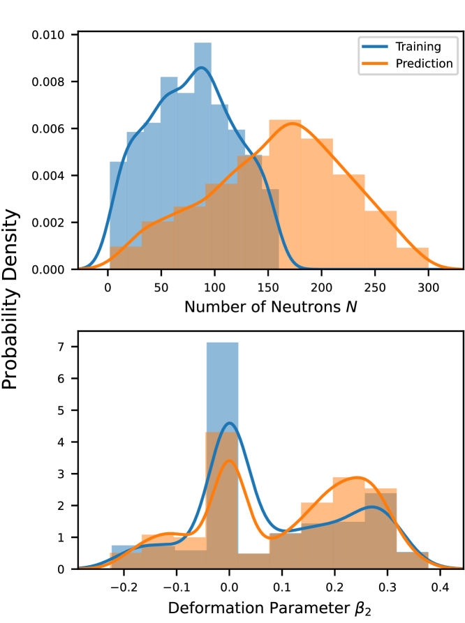
Mass tables of even-even nuclei were generated for each EDF using the numerical solver HFBTHO [42]. This means that we have samples for each property instead of a probability distribution function. We employ Kernel Density Estimation (KDE) [43, 44, 45] to obtain a reliable representation of the probability distribution function of each property. Figure 1 shows the samples and probability distribution functions for and for the deformation parameter calculated across the nuclear chart with the UNEDF0 functional. Blue corresponds to all even-even nuclei in the AME2020 mass evaluation data set [17, 18] and orange to all even-even nuclei between the proton and neutron driplines that are not in the AME2020 data set. The figure shows that using the neutron number () as a feature for training would require extrapolations when making predictions with the AI/ML algorithm. In contrast, using () as a feature does not require an extrapolation since the distributions in the training and prediction regions are fairly similar. For the SPA, we use as features only those properties with , where is an arbitrary cut-off.
We use random forest regression to evaluate the performance of each feature selection method [46]. A random forest is a collection of decision trees where each tree is trained with a random subset of all training data. The output of the random forest is the average output of all decision trees. This technique avoids the overfitting that a few outliers can cause on a single decision tree. Additionally, random forests have few hyperparameters to tune, which makes them ideal for validation studies like the one presented here; for a complete introduction to random forest regression and classification we refer the interested readers to [47] and [48]. Although the work presented here uses random forests, the concept of feature selection for extrapolation can be used with any other AI/ML algorithm.
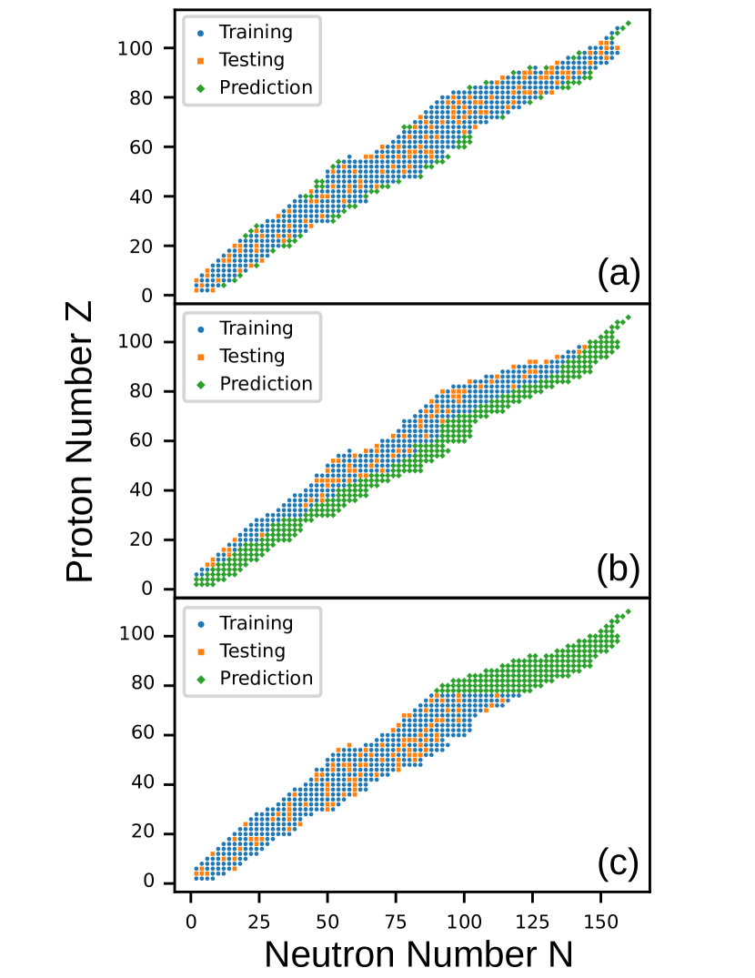

Results - We test the performance of our three feature selection approaches with available data. To this end, we define three prediction regions, which contain measured nuclei only, for which we will compare the estimated bias against the actual bias. The first region, dubbed time-wise split (TWS), consists of all the 70 even-even nuclei in the AME2020 data set that are not in the AME2003 data set [49, 50]. This simulates a realistic scenario in which predictions are tested over time as new measurements become available but does not test predictions far away from the training data. The second region, dubbed large-N split (LNS), consists of the up to most neutron-rich even-even nuclei in each isotopic chain present in the AME2020 data set. This scenario tests predictions towards neutron-rich nuclei but still remains relatively close to the training data. The third region, called large-Z split (LZS), consists of all even-even nuclei in AME2020 with . This scenario will test predictions far away from the training data. In each case the training/testing region consists of all even-even nuclei in AME2020 that are not present in the corresponding prediction region. The split between training and testing data is performed by randomly selecting 20% nuclei for testing and leaving the remaining 80% for training. Figure 2 shows the training, testing and prediction regions as described above. Note that changing the prediction region changes the distribution of each property and it is thus necessary to recalculate the Bhattacharyya coefficient in order to re-select a new set of features with . As mentioned earlier the cut-off is somewhat arbitrary and an optimal value depends on the value of all available properties. We set a cut-off of and in the TWS and LNS cases respectively since most properties have large values: a lower cut-off would include most properties as features and would not allow distinguishing between the APA and SPA scenarios. For the LZS case we allow for a more “lenient” cut-off of since there is a wider spread in the values among all properties.
We quantify the performance of a theoretical model for binding energies by calculating the root mean square error (rmse) , where is the total number of nuclides in a particular region. To estimate the quality of the corrected model after removing the bias (1), we then define the improvement index where is the rmse of the original EDF model and the one after removing the bias. Values mean that removing the bias has reduced the rmse; values mean that this modification has increased the rmse. Figure 3 shows the improvement index for the two EDFs considered in this work after removing the estimated bias with the three different feature selection methods. As expected, in the training region, irrespective of the EDF, the type of data analyzed and the feature selection method. In the testing region, the improvement is less pronounced but in general stays lower than 0.5. Results in the prediction region are somewhat comparable to, or slightly worse than, in the testing region when looking at data not too far from the training region (blue and orange) as already noticed in [22]. When making predictions far from the training region (green), however, the improvement index takes values greater than 1 for the UNEDF0 functional for the DA and APA feature selection methods. This means that removing the AI/ML-estimated bias has in fact degraded the predictive power of the model. Similar results are obtained for the UNEDF1HFB functional [51]. Only by carefully selecting features with large coefficients can we avoid this situation and keep . The case of SLy4 sheds additional light on this mechanism. The error on binding energies comes mostly from not removing the effect of the electronic correction in the fit of the EDF. As a result, it is rather large and has a very clear dependency on ; see Fig. 2 (b) in the Supplemental material [51]. This trend can be easily learned by the AI/ML model, and the resulting bias estimate is robust (as a function of ), accounts for most of the error and, therefore, still gives significant improvements in the prediction region, even far from training data. Put another way, feature selection is especially relevant for models with good predictive power with no clear the dependency of the model discrepancy on available properties.
Conclusions - We have analyzed the performance of three feature selection approaches to estimate the bias in DFT binding energies with two different EDFs. The performance of each approach was evaluated with three different splits of available data between training, testing and prediction. We showed that the direct approach, which uses and as the only features, produces reliable predictions only for nuclei that are close to the available training data. When making predictions at values of far away from the training data, removing the estimated bias can in fact reduce the accuracy of the DFT prediction. By selecting features with similar distributions in the training and prediction regions, our approach eliminates the need to extrapolate features when making predictions. It is the only one that consistently showed improvement among all three EDFs considered here and in all three splittings between training, testing and prediction data. While we demonstrated our feature-selection technique on nuclear binding energies computed from DFT, it could be generalized to any other observable and any other global theoretical model as long as enough training data and potential features are available. In fact, it is also potentially applicable in every scientific discipline (i) that rely on approximate theoretical models with adjustable parameters and (ii) where extrapolations outside measured data are needed.
Acknowledgements.
Discussions with M. Grosskopf, E. Lawrence, S. Wild and J. O’Neal are gratefully acknowledged. Support for this work was partly provided through Scientific Discovery through Advanced Computing (SciDAC) program funded by U.S. Department of Energy, Office of Science, Advanced Scientific Computing Research and Nuclear Physics. It was partly performed under the auspices of the US Department of Energy by the Lawrence Livermore National Laboratory under Contract DE-AC52-07NA27344. Computing support for this work came from the Lawrence Livermore National Laboratory (LLNL) Institutional Computing Grand Challenge program.References
- Giuliani et al. [2019] S. A. Giuliani, Z. Matheson, W. Nazarewicz, E. Olsen, P.-G. Reinhard, J. Sadhukhan, B. Schuetrumpf, N. Schunck, and P. Schwerdtfeger, Rev. Mod. Phys. 91, 011001 (2019).
- Schunck and Regnier [2022] N. Schunck and D. Regnier, “Theory of nuclear fission,” (2022), arXiv:2201.02719 [nucl-th] .
- Cowan et al. [2021] J. J. Cowan, C. Sneden, J. E. Lawler, A. Aprahamian, M. Wiescher, K. Langanke, G. Martínez-Pinedo, and F.-K. Thielemann, Rev. Mod. Phys. 93, 015002 (2021).
- Balantekin et al. [2014] A. B. Balantekin, J. Carlson, D. J. Dean, G. M. Fuller, R. J. Furnstahl, M. Hjorth-Jensen, R. V. F. Janssens, B.-A. Li, W. Nazarewicz, F. M. Nunes, W. E. Ormand, S. Reddy, and B. M. Sherrill, Mod. Phys. Lett. A 29, 1430010 (2014).
- Bohr and Mottelson [1998] A. Bohr and B. Mottelson, Nuclear Structure, Vol. I, Single-Particle Motion (World Scientific, 1998).
- Ring and Schuck [2004] P. Ring and P. Schuck, The Nuclear Many-Body Problem, Texts and Monographs in Physics (Springer, 2004).
- Weinberg [1990] S. Weinberg, Phys. Lett. B 251, 288 (1990).
- Machleidt and Sammarruca [2016] R. Machleidt and F. Sammarruca, Phys. Scr. 91, 083007 (2016).
- Hammer et al. [2020] H.-W. Hammer, S. König, and U. van Kolck, Rev. Mod. Phys. 92, 025004 (2020).
- Hagen et al. [2014] G. Hagen, T. Papenbrock, M. Hjorth-Jensen, and D. J. Dean, Rep. Prog. Phys. 77, 096302 (2014).
- Carlson et al. [2015] J. Carlson, S. Gandolfi, F. Pederiva, S. C. Pieper, R. Schiavilla, K. E. Schmidt, and R. B. Wiringa, Rev. Mod. Phys. 87, 1067 (2015).
- Hergert et al. [2016] H. Hergert, S. K. Bogner, T. D. Morris, A. Schwenk, and K. Tsukiyama, Phys. Rep. Memorial Volume in Honor of Gerald E. Brown, 621, 165 (2016).
- Stroberg et al. [2019] S. R. Stroberg, H. Hergert, S. K. Bogner, and J. D. Holt, Annu. Rev. Nucl. Part. Sci. 69, 307 (2019).
- Schunck et al. [2019] N. Schunck, M. Bender, A. Bulgac, T. Duguet, J.-P. Ebran, J. Engel, M. F. Michael, M. Kortelainen, and T. Nakatsukasa, Energy Density Functional Methods for Atomic Nuclei (Institute of Physics Publishing, 2019).
- Möller et al. [2016] P. Möller, A. J. Sierk, T. Ichikawa, and H. Sagawa, Atom. Data Nuc. Data Tab. 109, 1 (2016).
- Goriely et al. [2013] S. Goriely, N. Chamel, and J. M. Pearson, Phys. Rev. C 88, 061302 (2013).
- Huang et al. [2021] W. J. Huang, M. Wang, F. G. Kondev, G. Audi, and S. Naimi, Chinese Phys. C 45, 030002 (2021).
- Wang et al. [2021] M. Wang, W. J. Huang, F. G. Kondev, G. Audi, and S. Naimi, Chinese Phys. C 45, 030003 (2021).
- Utama et al. [2016] R. Utama, J. Piekarewicz, and H. B. Prosper, Phys. Rev. C 93, 014311 (2016).
- Utama and Piekarewicz [2017] R. Utama and J. Piekarewicz, Phys. Rev. C 96, 044308 (2017).
- Utama and Piekarewicz [2018] R. Utama and J. Piekarewicz, Phys. Rev. C 97, 014306 (2018).
- Neufcourt et al. [2018] L. Neufcourt, Y. Cao, W. Nazarewicz, and F. Viens, Phys. Rev. C 98, 034318 (2018).
- Neufcourt et al. [2019] L. Neufcourt, Y. Cao, W. Nazarewicz, E. Olsen, and F. Viens, Phys. Rev. Lett. 122, 062502 (2019).
- Kejzlar et al. [2019] V. Kejzlar, L. Neufcourt, T. Maiti, and F. Viens, (2019), arXiv:1904.04793 .
- Jiang et al. [2019] W. G. Jiang, G. Hagen, and T. Papenbrock, Phys. Rev. C 100, 054326 (2019).
- Niu et al. [2019] Z. M. Niu, H. Z. Liang, B. H. Sun, W. H. Long, and Y. F. Niu, Phys. Rev. C 99, 064307 (2019).
- Wang et al. [2019] Z.-A. Wang, J. Pei, Y. Liu, and Y. Qiang, Phys. Rev. Lett. 123, 122501 (2019).
- Lasseri et al. [2020] R.-D. Lasseri, D. Regnier, J.-P. Ebran, and A. Penon, Phys. Rev. Lett. 124, 162502 (2020).
- Keeble and Rios [2020] J. W. T. Keeble and A. Rios, Physics Letters B 809, 135743 (2020).
- Neufcourt et al. [2020] L. Neufcourt, Y. Cao, S. A. Giuliani, W. Nazarewicz, E. Olsen, and O. B. Tarasov, Phys. Rev. C 101, 044307 (2020).
- Bedaque et al. [2021] P. Bedaque, A. Boehnlein, M. Cromaz, M. Diefenthaler, L. Elouadrhiri, T. Horn, M. Kuchera, D. Lawrence, D. Lee, S. Lidia, R. McKeown, W. Melnitchouk, W. Nazarewicz, K. Orginos, Y. Roblin, M. Scott Smith, M. Schram, and X.-N. Wang, Eur. Phys. J. A 57, 100 (2021).
- Haley and Soloway [1992] P. Haley and D. Soloway, in [Proceedings 1992] IJCNN International Joint Conference on Neural Networks, Vol. 4 (1992) pp. 25–30 vol.4.
- Chabanat et al. [1998] E. Chabanat, P. Bonche, P. Haensel, J. Meyer, and R. Schaeffer, Nucl. Phys. A 635, 231 (1998).
- Kortelainen et al. [2010] M. Kortelainen, T. Lesinski, J. Moré, W. Nazarewicz, J. Sarich, N. Schunck, M. V. Stoitsov, and S. Wild, Phys. Rev. C 82, 024313 (2010).
- Schunck et al. [2015] N. Schunck, J. D. McDonnell, J. Sarich, S. M. Wild, and D. Higdon, J. Phys. G: Nucl. Part. Phys. 42, 034024 (2015).
- JETSCAPE Collaboration et al. [2021] JETSCAPE Collaboration, D. Everett, W. Ke, J.-F. Paquet, G. Vujanovic, S. A. Bass, L. Du, C. Gale, M. Heffernan, U. Heinz, D. Liyanage, M. Luzum, A. Majumder, M. McNelis, C. Shen, Y. Xu, A. Angerami, S. Cao, Y. Chen, J. Coleman, L. Cunqueiro, T. Dai, R. Ehlers, H. Elfner, W. Fan, R. J. Fries, F. Garza, Y. He, B. V. Jacak, P. M. Jacobs, S. Jeon, B. Kim, M. Kordell, A. Kumar, S. Mak, J. Mulligan, C. Nattrass, D. Oliinychenko, C. Park, J. H. Putschke, G. Roland, B. Schenke, L. Schwiebert, A. Silva, C. Sirimanna, R. A. Soltz, Y. Tachibana, X.-N. Wang, and R. L. Wolpert, Phys. Rev. C 103, 054904 (2021).
- Bhattacharyya [1946] A. Bhattacharyya, Sankhyā: The Indian Journal of Statistics (1933-1960) 7, 401 (1946).
- Niigaki et al. [2012] H. Niigaki, J. Shimamura, and M. Morimoto, in Proceedings of the 21st International Conference on Pattern Recognition (ICPR2012) (2012) pp. 2009–2012.
- Patra et al. [2015] B. K. Patra, R. Launonen, V. Ollikainen, and S. Nandi, Knowledge-Based Systems 82, 163 (2015).
- Singh et al. [2020] P. K. Singh, M. Sinha, S. Das, and P. Choudhury, Appl Intell 50, 4708 (2020).
- Van Molle et al. [2021] P. Van Molle, T. Verbelen, B. Vankeirsbilck, J. De Vylder, B. Diricx, T. Kimpe, P. Simoens, and B. Dhoedt, Neural Comput & Applic 33, 10259 (2021).
- Navarro Pérez et al. [2017] R. Navarro Pérez, N. Schunck, R. D. Lasseri, C. Zhang, and J. Sarich, Computer Physics Communications 220, 363 (2017).
- Rosenblatt [1956] M. Rosenblatt, The Annals of Mathematical Statistics 27, 832 (1956).
- Parzen [1962] E. Parzen, The Annals of Mathematical Statistics 33, 1065 (1962).
- Gramacki [2017] A. Gramacki, Nonparametric Kernel Density Estimation and Its Computational Aspects (Springer, 2017).
- Breiman [2001] L. Breiman, Machine Learning 45, 5 (2001).
- Biau and Scornet [2016] G. Biau and E. Scornet, TEST 25, 197 (2016).
- Genuer and Poggi [2020] R. Genuer and J.-M. Poggi, Random Forests with R (Springer Nature, 2020).
- Audi et al. [2003] G. Audi, A. H. Wapstra, and C. Thibault, Nucl. Phys. A The 2003 NUBASE and Atomic Mass Evaluations, 729, 337 (2003).
- Wapstra et al. [2003] A. H. Wapstra, G. Audi, and C. Thibault, Nucl. Sci. Eng. The 2003 NUBASE and Atomic Mass Evaluations, 729, 129 (2003).
- [51] See Supplemental Material.