Consequences of the compatibility of skein algebra and cluster algebra on surfaces
Abstract.
We investigate two algebra of curves on a topological surface with interior punctures – the cluster algebra of surfaces defined by Fomin, Shapiro, and Thurston, and the generalized skein algebra constructed by Roger and Yang. By establishing their compatibility, we resolve Roger-Yang’s conjecture on the deformation quantization of the decorated Teichmüller space. We also obtain several structural results on the cluster algebra of surfaces. The cluster algebra of a positive genus surface is not finitely generated, and it differs from its upper cluster algebra.
1. Introduction
By a surface , we denote a compact Riemann surface of genus , without boundaries, minus punctures. We may associate two ‘algebras of curves’ on , but coming from entirely different motivations – one from geometric topology, and the other from combinatorial algebra. In this paper, we establish compatibility between the two algebras. By employing it, we prove several structural results about each of the algebras that might not be readily apparent if considering each algebra separately.
The first algebra is the curve algebra , which belongs to a family of invariants of surfaces that are related to the Jones polynomial for knots [Jon85] and to the Witten-Reshetikhin-Turaev topological quantum field theory [Wit89, RT91, BHMV95]. The most well-studied of this family is the Kauffman bracket skein algebra of an unpunctured surface [Prz91, Tur91]. It is known to be related to hyperbolic geometry— the skein algebra is the deformation quantization of the -character variety, which contains the Teichmüller space of the surface [Tur91, Bul97, BFKB99, PS00]. In [RY14], Roger and Yang sought to generalize this relationship between the skein algebra and the Teichmüller space to the case of a punctured surface. For a punctured surface , they defined a generalized skein algebra spanned by disjoint unions of framed knots, arcs, and vertex classes. They proposed that it should be the deformation quantization for the decorated Teichmüller space constructed by Penner in [Pen87, Pen92]. The curve algebra we study in this paper is the classical limit of Roger-Yang’s generalized skein algebra obtained by setting .
The second algebra studied in this paper is the cluster algebra of a surface. Such cluster algebras were observed by [GSV05, FST08] to be interesting examples of the cluster algebras originally introduced by Fomin and Zelevinsky in [FZ02] for studying the total positivity and dual canonical bases in Lie theory. Defined for any punctured surface admitting an ideal triangulation, the cluster algebra is generated by arcs with tagging (of plain or notched) at its endpoints. From the combinatorial perspective, the tagging is needed for to have the structure of a cluster algebra, and various geometric interpretations can be seen from [FG06, MSW11, FT18, AB20]. This paper was started in part from the authors’ attempt to better understand the relationship between the two algebras.
Each of the two algebra has its own distinct features, and the main results of this paper follow from transferring advantageous properties from one algebra to another. Our primary tool is an injective homomorphism from the curve algebra to the cluster algebra , which manifests the ‘compatibility’ of the two commutative algebras. By leveraging the integrality of , we prove that the generalized skein algebra is a deformation quantization of and resolve Roger-Yang’s conjecture (Theorem A). Compatibility also enables us to define a nontrivial ‘reduction’ map and prove the non-finite generation of (Theorem C) for . The unifying theme of this paper is the interplay between the two algebras afforded by compatibility.
1.1. Compatibility of curve algebra and cluster algebra
Let be a Riemann surface of genus with punctures. We assume that , so that -punctured spheres with are excluded. When we define the cluster algebra, we also exclude the three-punctured sphere.
We have an explicit comparison of and , which will be the key step to the main results of this paper.
Compatibility Lemma.
Let be the cluster algebra and be the curve algebra associated to . Then there is a monomorphism
This is not merely an existence statement. As discussed in Section 4, the construction of gives a simple geometric interpretation of the tagging, which can be plain or notched (Definition 4.1). The upshot is that “a notch is a vertex class,” where a vertex class is a formal variable in assigned to each puncture (Definition 2.1).
Both algebras have their geometric origin from the same decorated Teichmüller space due to Penner, and the proof of the Compatibility Lemma is relatively straightforward (see Section 4). Indeed, a similar compatibility result for surfaces with boundaries but without interior punctures was proven by Muller in [Mul16]. We note that in because there are no interior punctures, the vertex classes in the skein algebra and the tagged arcs in the cluster algebra do not exist, and thus the interpretation of the tagging as a vertex is new in the punctured surface case.
Like other recent developments [BMS22, HI15, LS19, NT20, Yac19], one could think of these compatibility results as another indication of deep connection between knot theory and cluster algebra. Instead, what we would rather emphasize here is the key role the Compatibility Lemma plays in the proofs of the main results of this paper, as we will see throughout the paper. Let us now describe the main results in this paper, beginning first with the quantum theory of skein algebras and then turning to the structural theory of cluster algebras.
1.2. Skein algebra and deformation quantization
In [RY14], Roger and Yang introduced a generalized skein algebra as a candidate of the deformation quantization of . Their program consists of two steps. First, they showed that is a deformation of quantization of its classical limit . They then proved that there is a Poisson algebra homomorphism whose Poisson structures are given by the generalized Goldman bracket and the Weil-Peterssen form, respectively [RY14, Theorem 1.2]. Thus, if the Poisson algebra representation is faithful (meaning is injective), then can be understood as the quantization of . However, they left the faithfulness as a conjecture [RY14, Conjecture 3.4]. In Section 5, we prove it by employing Compatibility Lemma and finish Roger and Yang’s program.
Theorem A.
The Roger-Yang generalized skein algebra is a deformation quantization of the decorated Teichmüller space .
Moreover, a consequence of our proof of Theorem A is that the fractional algebras of both the two algebras and are identical. It thus follows that
Theorem B.
The Roger-Yang generalized skein algebra is a deformation quantization of .
Note that in our earlier paper [MW21], we already showed that Theorem A hold when is relatively large compared to [MW21, Theorem B]. The proof was based on a long diagramatical computation with little theoretical support nor intuition. We find that our proofs here, based on the relationship with cluster algebras established by Compatibility Lemma, provides a more satisfactory theoretical reasoning.
Remark 1.1.
In [Mul16], Muller has a similar result as Theorem B in the case of surfaces with boundaries but without punctures, resulting in a quantization where arcs -commute. However, Muller’s method cannot apply in the case considered in this paper, because does not extend to a quantum cluster algebra of Berenstein-Zelevinski [BZ05] if there is an interior puncture (see Remark 3.14 for a more in depth discussion). Instead, the quantization of Theorems A and B use the Poisson structure for the Roger-Yang skein algebra based on Mondello’s computation for -length of arcs [Mon09]. In particular, these -lengths do not form log canonical coordinates in the sense of [GSV05, Section 2.2]. Hence arcs are not -commutative in the quantization, but satisfy a two-term skein relation that generalizes the Ptolemy exchange relations for cluster variables.
1.3. Comparison of cluster algebras with their upper cluster algebra
The upper cluster algebra (Definition 3.2) contains the ordinary cluster algebra and is constructed from the same combinatorial data of seed. In many ways, behaves better than , and thus the question of whether or not has attracted many researchers in the cluster algebra community. For the summary of some known results, see [CLS15, Section 1.2] and a very recent result [IOS23]. For , when , it was shown that by Ladkani [Lad13].
Here, we use the curve algebra and a variation (Definition 2.10), and obtain an inclusion
| (1.1) |
The algebra is a subalgebra of generated by the image of and the Kauffman bracket skein algebra of generated by isotopy classes of loops. We conjecture that (Conjecture 6.16). However, to the authors’ knowledge, it is still unknown if the ‘geometric’ subalgebra generated by tagged arcs and loops coincide with . See Remark 6.15. For the comparison of and , see Remark 6.14.
1.4. Determining whether cluster algebras are finitely generated
It is known that the Roger-Yang skein algebra is finitely generated [BKPW16a], and our method is to use the compatibility map to deduce results about the cluster algebra.
By [Lad13], it is known that is not finitely generated for all . We prove the following:
Theorem C.
The cluster algebra of a sphere is finitely generated. On the other hand, for , is not finitely generated.
Note that the cluster algebra is defined only when a surface has punctures, so for all cases. And in the case of a sphere, we additionally require punctures. From Theorem C and (1.1), we have the immediate corollary:
Theorem D.
For every , .
1.5. Structure of the paper
Sections 2 and 3 are review of the definition and basic properties of and , respectively, and related constructions. In Section 4, we start with the compatibility map , and show that is well-defined and injective. The next two sections detail our main results—Section 5 establishes the curve algebra as a quantization of decorated Teichmuller space, and Section 6 discusses algebraic properties of the cluster algebra and upper cluster algebra.
Acknowledgement.
The authors would like to thank to Wade Bloomquist, Hyunkyu Kim, Thang Le, Kyungyong Lee, Gregg Musiker, Fan Qin, and Dylan Thurston for valuable conversations. This work was completed while the first author was visiting Stanford University. He gratefully appreciates the hospitality during his visit. The second author is partially supported by grant DMS-1906323 from the US National Science Foundation and a Birman Fellowship from the American Mathematical Society.
2. The curve algebra
In this section, we give a formal definition and basic properties of the curve algebra . For details, see [RY14, Section 2.2] and [MW21, Section 2.4].
In this paper, a surface is , where is a Riemann surface of genus without boundary, and is a finite set of points in . We call the set of punctures or vertices.
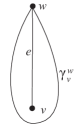
A loop on is an immersion of a circle into . An arc in is an immersion of into such that the image of is in and the image of two endpoints are (not necessarily distinct) points in . The seemingly unnecessary underbar notation will be justified in Section 3.
Definition 2.1.
Let be a commutative ring. The curve algebra is the -algebra generated by isotopy classes of loops, arcs, , and their formal inverses , modded out by the following relations:
| (1) | (Skein relation) | |
| (2) | (Puncture-skein relation) | |
| (3) | (Framing relation) | |
| (4) | (Puncture-framing relation) | . |
The multiplication of elements in are represented by taking the union of generators (and counted with multiplicity). We allow the empty curve and it is the multiplicative identity. In the relations, the curves are assumed to be identical outside of the small balls depicted, and the -th puncture is depicted in the second relation.
We set , so that we mean by default. Then .
Remark 2.2.
Note that in the curve algebra originally discussed by Roger-Yang [RY14], they used , and the vertices were treated as coefficients. But for our purpose, it is more natural to think of the vertices as generators of the algebra.
Remark 2.3.
One might wonder about our choice of coefficient ring , as compared to Roger and Yang’s choice of . Clearly, there is a morphism . In addition, one can adapt the proof of [RY14, Theorem 2.4] by replacing the -coefficient by the -coefficient to show that (with -coefficients) has no torsion. Thus, we have an inclusion . It follows, for example, that if is an integral domain, then is also an integral domain.
Example 2.4.
Let be an arc bounding an unpunctured monogon with the vertex . Then we can compute as follows:
Since is invertible in , this shows that any arc bounding an unpunctured monogon is zero in .
Lemma 2.5.
Let and be two distinct punctures, and be an arc connecting and . In addition, let be an arc with both ends at that bounds a one-punctured monogon containing . Then .
Proof.
since any arc bounding an unpunctured monogon in by the example above. ∎
2.1. Relationship of with hyperbolic geometry
Let be the decorated Teichmüller space of constructed by Penner [Pen87]. It parameterizes all pairs where is a complete hyperbolic metric and is a choice of a horocycle at every puncture of . Given such a pair , one can assign a well-defined length to any loop on and any arc that goes from puncture to puncture on . In addition, we set the length of a vertex to be the length of the horocycle around that vertex. These lengths of loops, arcs, and vertices can then be used to define -length functions on , and it was shown in [Pen87] that the -length functions parametrize the ring of -valued functions on . These -length functions can be used to define a Poisson structure on induced by the Weil-Petersson form [Pen92].
Roger and Yang defined the curve algebra and showed ([RY14, Theorem 1.2]) that there is a Poisson algebra homomorphism
| (2.1) |
that sends any loop, arc, or vertex to its corresponding -length function. One can think of the relations from the curve algebra as designed to mirror the relations from the -length functions in . In fact, Roger and Yang conjectured that the curve algebra relations captures all of the relations from , or equivalently, that
Theorem A of this paper proves Roger and Yang’s conjecture in all cases, by appealing to the algebraic properties of and the following theorem:
Theorem 2.7 ([MW21, Theorem A]).
If is an integral domain, then is injective.
In previous work [MW21, Theorem B and Section 4] , we were able to verify that is an integral domain when admits a ‘locally planar’ ideal triangulation. In particular, the genus and the number of punctures should satisfy
In Theorem 5.2 of this paper, we instead use cluster algebras to obtain an independent and unconditional proof of integrality, so that Conjecture 2.6 applies for any .
2.2. Relationship of with Kauffman bracket skein algebra
Roger and Yang’s definition of the curve algebra and the construction of in [RY14] was motivated by a search for an appropriate quantization of the decorated Teichmuller space . In particular, they wanted to mimic and generalize the set-up of [Tur91, Bul97, BFKB99, PS00] that establishes the Kauffman bracket skein algebra as a quantization of the -character variety of , which contains the Teichmüller space as a dense open subspace. Towards this goal, Roger and Yang defined a generalized Goldman bracket for and used it to define a deformation quantization that we here denote by [RY14, Theorem 1.1].
We omit the precise definition of , but instead mention some key properties. Firstly, is an -algebra generated by arcs, loops, and vertices, and reduces to the usual Kauffman bracket skein algebra in the absence of punctures (so that the puncture-skein and puncture-framing relations can be ignored). For this reason, we will refer to Roger-Yang’s as a skein algebra. In addition, can be identified with when .
As stated in Theorem A, establishment of Conjecture 2.6 implies that is indeed a quantization of , completing Roger and Yang’s original goal. Moreover, many of the results about the curve algebra have consequences for the skein algebra . For example, it was proved in [MW21, Theorem C] that if is an integral domain, then is also an integral domain.
Conversely, many results about also apply to . The following two theorems about algebraic properties of were proved for with -coefficients, but the same proof works just as well for -coefficients and with .
Theorem 2.8 ([BKPW16a, Theorem 2.2]).
The algebra is finitely generated.
We now turn to the case. Let be a small circle on . We may assume that the punctures lie on in the clockwise circular order. Let be the simple arc in the disk bounded by that connects and .
Theorem 2.9 ([ACDHM21, Theorem 1.1]).
The algebra is isomorphic to
where is an ideal generated by
-
(1)
for any 4-subset in cyclic order;
-
(2)
;
-
(3)
,
where and are explicit polynomials in the generators (and have a geometric description).
For definitions of and and formulas in terms of , see [ACDHM21, Section 4].
2.3. A useful variation of
Definition 2.10.
Let be the subalgebra generated by the following elements:
-
(1)
Isotopy classes of loops;
-
(2)
, , , and , where is an arc connecting (possibly non-distinct) vertices and .
For any coefficient ring , set . Later, we will need a slight extension/variation of Theorem 2.8.
Theorem 2.11.
For any coefficient ring , the algebra is finitely generated.
The proof is identical to that of [BKPW16a, Theorem 2.2]. More specifically, one uses a generalized handle decomposition of with a disk removed. The complexity of a curve is defined based on how many times and in what manner a minimal representation of the curve traverses the handles [BKPW16a, Section 3.1]. By application of skein identities, it is shown that any curve can be recursively written as lower-complexity curves [BKPW16a, Lemmas 3.1–3.4]. Importantly, none of the skein identities in the recursive steps use the formal inverses of vertices. In particular, the skein identities from [BKPW16a, Lemmas 3.1 and 3.2]) involve only undecorated arcs of the form , and those for [BKPW16a, Lemma 3.3] uses arcs of the form and . For [BKPW16a, Lemma 3.4], one identity (first identity on [BKPW16a, p.10] ) involves . However, the recursive step comes from substituting it into a previous equation (last identify on [BKPW16a, p.9]), in a term with a factor of . Because of the cancellation, the recursive step can be written in a form involving only undecorated arcs.
Remark 2.12.
Later, we will see that the cluster algebra (to be defined in Section 3) can be understood as a subalgebra generated by ‘tagged’ arc classes by Compatibility Lemma. On the other hand, the classical limit () of the original Kauffman bracket skein algebra [Prz91, Tur91] is a subalgebra of generated by loop classes. So, one may interpret as the subalgebra of generated by the image of the cluster algebra and the usual Kauffman bracket skein algebra.
3. Cluster algebra from surfaces
We review the definition of the cluster algebra constructed from a punctured surface , as introduced by Fomin, Shapiro, and Thurston in [FST08].
3.1. Definition of cluster algebras
We begin by noting that we will not need the definition of cluster algebras in full generality, which can be found for example in [FZ02]. We will restrict to the case of constant coefficient, skew-symmetric exchange matrix, and no frozen variables. The only minor extension is that we allow more general base ring including finite field, while in many literature a cluster algebra is defined over , , , or . Essentially the choice of coefficient ring does not significantly impact the theory [BMRS15, Section 2].
Let be an integral domain. Let be a purely transcendental finite extension of , the field of fraction of . A seed is a pair , where is a free generating set for as a field over and is a skew-symmetric integral matrix. is called the exchange matrix, the set is the cluster, and its elements are the cluster variables of the seed.
For a seed and , a mutation in the direction of is an operation that produces another seed where
-
(1)
is such that is defined by the exchange relation
and all other cluster variables are identical, so for ;
-
(2)
is defined by
(3.1)
Sometimes we notate it as . It is straightforward to check that a mutation is involutive.
Since a mutation of a seed produces another seed, repeated mutations can be performed following any sequence of indices . We say that two seeds and are mutation equivalent and write if one seed can be obtained from the other by a sequence of mutations.
Definition 3.1.
The cluster algebra is the -subalgebra of the ambient field generated by
the cluster variables of seeds that are mutation equivalent to a seed . Since mutation equivalent seeds produce the same cluster algebra, we write instead of when the choice of initial seed may be safely suppressed. When we need to specify the coefficient ring, we use the notation for .
A simplicial complex, called the cluster complex of , is often used to describe the relationships between the cluster variables used to generate it. In particular, the vertices of the cluster complex are the cluster variables that generate , and there is a -simplex whenever cluster variables belong to the same cluster. Thus each seed in a cluster algebra gives rise to a maximal simplex in the cluster complex. The exhange graph is the dual graph, where the vertices are the seeds, and there is an edge between two seeds if they are mutations of each other. So by definition, the exchange graph of a cluster algebra must be an -regular, connected graph.
By the Laurent phenomenon [FZ02, Theorem 3.1], for any and an equivalent seed ,
Definition 3.2.
For a cluster algebra , the upper cluster algebra is defined by
The Laurent phenomenon tells that . In general they do not coincide. The upper cluster algebra behaves better than ; for example, is an integrally closed domain if is [BMRS15, Lemma 2.1]. However, the computation of and the question of whether or not are in general difficult. For a partial criterion for , see [Mul13].
3.2. Definition of the cluster algebra of a surface
In this paper, we focus exclusively on cluster algebras associated to a punctured surface . The cluster algebra is essentially the algebra generated by isotopy classes of arcs on the surface . Each cluster should come from the arc classes in a maximal compatible set; in other words, the edges of a triangulation should form a cluster. A mutation should correspond to a flip of an edge of the triangulation. Although this idea is sufficient to define , the intuitive picture is not complete as stands, because not every arc in an ordinary triangulation is flippable if the triangulation contains a self-folded triangle. This problem was resolved in [FST08] by introducing tagged arcs.
We begin with a review of ordinary triangulations, and how the data from a single triangulation without a self-folded triangle is sufficient to define a cluster algebra . We then introduce tagged triangulations, which will fully describe the correspondence between cluster variables and tagged arcs. The results in [FST08] also apply to surfaces with boundary and marked points on the boundary, but we do not need that generality here.
3.2.1. Ordinary Triangulations
As in Section 2, we denote a punctured surface without boundary by , where . We assume that , and exclude for .
Recall an arc of is an immersion such that embeds in and takes the endpoints to the punctures . The set of isotopy classes of arcs connecting two punctures in will be denoted by . Two arcs are said to be compatible if they are the same, or if they do not intersect except at the punctures. A maximal collection of distinct, pairwise compatible isotopy classes of arcs forms an ideal triangulation on . The arcs in a triangulation are referred to as edges, and the set of edges is denoted by . Because of maximality, separates into a set of triangles, which is denoted by . Recall that , and from now on, we let .
A flip is an operation that removes an arc from a triangulation , replaces it by another compatible arc, so results in another triangulation . So and share all arcs except one. Note that not every arc in a triangulation is flippable; in particular, the folded edge in a self-folded triangle is not flippable. However, there is a finite sequence of flips that transforms any triangulation into one without self-folded triangles, and more generally, any two triangulations can be connected by finitely many flips.
Let the arc complex be the abstract simplicial complex where a -simplex is a collection of distinct, mutually compatible arcs in . Thus each vertex is an isotopy class of an arc, and a maximal simplex corresponds to a triangulation . Its dual graph we denote by . Equivalently, is the graph whose vertices are the ideal triangulations of and two vertices are connected if and only if the ideal triangulations are related by a flip. is connected in codimension-one, and is connected, with each vertex degree at most .
3.2.2. Cluster algebra from an ordinary triangulation
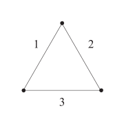
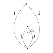
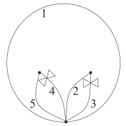
The combinatorial data from an ordinary triangulation can be encoded using a matrix, which we will define using puzzle pieces. Figure 3.1 shows three “puzzle pieces” which are intended to be glued together along their boundary edges in order to construct triangulations of surfaces. Figure 3.2 depicts a triangulation of the four-punctured sphere , where the exterior of three self-folded triangles is another triangle, which is not drawn in but which should be understood to be a part of the figure. We sometimes refer to the triangulation in Figure 3.2 as a fourth puzzle piece, even though it is not meant to be glued to any other puzzle piece. The matrix associated to the puzzle pieces are also given in Figures 3.1 and 3.2. Notice that there is one row and column for each edge in the puzzle piece, and all four matrices are skew-symmetric.
As shown in [FST08, Section 4], every triangulation of can be obtained from gluing puzzle pieces of the four types depicted in Figures 3.1 and 3.2. Moreover, there is a well-defined exchange matrix that is the matrix whose rows and columns are indexed by the edges of the triangulation, constructed as the sum of all minor matrices obtained from some set of puzzle pieces which can be used to construct . Since an edge of a triangulation can be contained in at most two puzzle pieces, the entries of the exchange matrix must satisfy for all . We refer the reader to [FST08] for details as well as worked examples.
 |
 |
 |
|
Observe that the exchange matrix is skew-symmetric, since the minor matrices obtained from the puzzle pieces are skew-symmetric. Thus, we may define the seed from the triangulation to be the pair , where is the set of edges of a triangulation and is its exchange matrix.
Proposition 3.3 ([FST08, Proposition 4.8]).
Suppose that the -th edge of a triangulation is flippable, and let be the result of flipping that edge. Then the exchange matrix for is the exchange matrix for mutated in the direction , i.e., .
Since any two triangulations of are related by a sequence of flips, seeds from any two triangulations of are related by a sequence of mutations and hence are mutation equivalent. Hence, we have:
Definition 3.4.
Let the cluster algebra of be defined as . Then is generated by the edges of triangulations of and hence is independent of the initial choice of triangulation .
However, the arcs are insufficient to describe all cluster variables. In a cluster algebra, we necessarily are able to mutate along every edge of a triangulation, but when the surface admits a triangulation with self-folded triangles, not every edge is flippable. In other words, for some vertex in , the degree might be strictly smaller than , while the exchange graph of has to be -regular. So, we can only in general say that is a subcomplex of the cluster complex, and is a subgraph of the cluster algebra’s exchange graph. To fill in this gap, Fomin, Shapiro, and Thurston [FST08] introduced a generalization of ordinary arcs which we describe next.
3.2.3. Tagged Triangulations
Definition 3.5.
A tagged arc on is an arc on along with one of two decorations, plain or notched, at each of the two ends of such that:
-
(1)
does not cut a one-punctured monogon;
-
(2)
if both ends of the arc are at the same vertex, then they have the same decoration.
The ordinary arc is the underlying arc of the tagged arc . The decoration of plain or notched at an end of a tagged arc is referred to as the tag at that end, or at the corresponding vertex. The set of isotopy classes of tagged arcs is denoted by . Naturally .
Many concepts and constructions for arcs can be extended to tagged arcs. Recall that two ordinary arcs are compatible if, up to isotopy, they are either the same or disjoint except at the vertices.
Definition 3.6.
If tagged arcs and satisfy the following conditions:
-
(1)
the underlying arcs are and are compatible; and
-
(2)
in the case that , then and have the same tag on at least one of the shared vertices;
-
(3)
in the case that and they share a vertex , then and have the same tag at .
then we say that and are compatible.
It follows from the definition that, if and are compatible tagged arcs whose underlying arcs are not the same but share both vertices, then and must have the same tag at each vertex. For example, on a one-punctured surface, all compatible arcs share a vertex, and hence all ends of compatible arcs must have the same tag.
Definition 3.7.
A tagged triangulation is a maximal collection of compatible, distinct tagged arcs.
If we take the arcs of an ordinary triangulation and tag all of the ends plainly, then we obtain a tagged triangulation. However, the converse is not true; it is possible that the underlying curves of a tagged triangulation do not form an ordinary triangulation of . In particular, tagged triangulations may cut out bigons as pictured on the right of Figure 3.3. Because such bigons appear often in tagged triangulations, we have the following language for describing them.
Definition 3.8.
Let and be two distinct vertices. A dangle is a bigon with vertices at and such that its two boundary arcs are compatible and have different tags at the vertex (Figure 3.3). The jewel of is the vertex with two distinct tags. An envelope of the dangle is the boundary of a one-punctured monogon that is based at and such that it encloses the jewel and has the same tags at as on .

Note that, because the two boundary arcs of a dangle are compatible and the tags at the jewel are different, the tags at the remaining vertex must be both plain or both notched. In a tagged triangulation, the jewel of a dangle cannot be the endpoint of any other edge besides those of the dangle, and thus the degree of the jewel is two.
Let the tagged arc complex be the abstract simplicial complex generated by compatible distinct tagged arcs in , and let be the dual graph of . Equivalently, is the graph whose vertices are the tagged triangulations of and two vertices are connected if and only if the tagged triangulations share all but one edge. An edge of corresponds to a tagged flip, which we think of as an operation that removes one tagged arc from the tagged triangulation and replaces it with a different compatible tagged arc.
Proposition 3.9 ([FST08, Proposition 7.10]).
Let be the number of edges of an ideal triangulation on .
When , is an -regular, connected graph. Every edge of a tagged triangulation is flippable and any two tagged triangulations is related by a sequence of tagged flips.
When , is an -regular graph with two isomorphic connected components, one where all tags are plain and one where all tags are notched.
It follows that is also connected when there are at least two punctures and has two isomorphic connected components when there is exactly one puncture. Note that in the case of one puncture, each connected component of is isomorphic to , and each component of the tagged arc complex is isomorphic to . For simplicity, we will restrict to the component where all tags are plain in the one puncture case for ease of exposition. With this convention, we have that both and are connected in all cases.
The relationship between the ordinary set-up and the tagged one can be described by a map , which we will define using the language of dangles and envelopes from Definition 3.8 and Figure 3.3. If is not an envelope (that is, it does not cut out a once-punctured monogon), then is tagged plain at both ends. If is an envelope based at and surrounding , then is the unique arc enclosed by that connects and and that is notched at . For example, in Figure 3.3, , but maps the envelope to the tagged arc on the right.
As shown in [FST08, Section 7], preserves the compatibility of arcs and provides a way of mapping an ordinary triangulation to a tagged triangulation. In this way, we can understand as a subcomplex of (though possibly it is not an induced subcomplex), and as a subgraph of .
To define the exchange matrix of a tagged triangulation, we again use puzzle pieces, as drawn in Figure 3.4. As before, the fourth puzzle piece by itself is a tagged triangulation of the four-punctured sphere . Since it does not have any exterior edge, it cannot be glued with any other puzzle pieces.
 |
 |
 |
 |
| A | B | C | D |
Lemma 3.10.
Any tagged triangulation on is obtained by
-
(1)
gluing the tagged puzzle pieces along their boundary edges; and
-
(2)
tagging all ends of the glued boundary edges in a compatible way.
Proof.
For the given tagged triangulation , we may think it as a top dimensional simplex in . Take a subsimplex , by eliminating all dangles. Then at each vertex of , the adjacent tagged arcs have the same tag.
Pick a region bounded by arcs in . It is sufficient to show that is one of the tagged puzzle pieces. is bounded by at most three arcs. Otherwise we can refine the triangulation by introducing a new tagged arc dividing the region , which violates the maximality of . There is no inner vertex except the other end of dangles, because otherwise we can insert another compatible tagged edge connecting and one of the boundary vertices. If has boundary arcs, then there are dangles in , by the maximality of . Then Figure 3.4 are the remaining possibilities. ∎
Observe that the four tagged puzzle pieces in Figure 3.4 are the images of the four ordinary puzzle pieces in Figures 3.1 and 3.2 under the map . We define the matrix associated to each tagged puzzle piece as the same one associated to its corresponding ordinary puzzle piece. Note when two tagged arcs have the same underlying arc, their corresponding matrix entries are the same.
Definition 3.11.
Let be a tagged triangulation with edges that is made up of tagged puzzle pieces, and let be the set of its edges. The exchange matrix is the matrix whose rows and columns are indexed by the edges, constructed as the sum of all minor matrices obtained from the puzzle pieces used to construct . The seed from the triangulation is the pair .
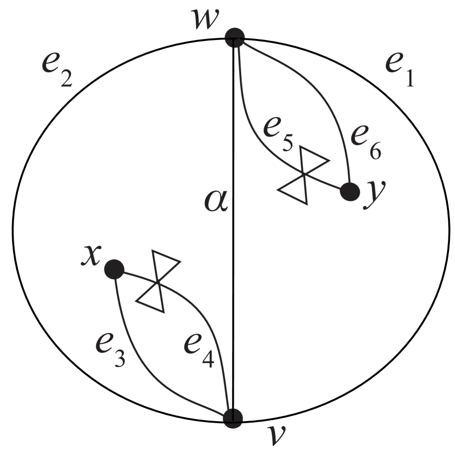
Example 3.12.
Consider the tagged triangulation of shown on the left of Figure 4.7. It is obtained from gluing together two puzzle pieces of Type B. Taking , the exchange matrix for the triangulation on the left is
Mutation of produces the triangulation on the right of Figure 4.7, which is by itself the Type D puzzle piece. The mutated exchange matrix is the one from Figure 3.2.
It is a straightforward calculation to check that the exchange matrix for the tagged triangulation obtained from flipping the -th edge of is the exchange matrix for mutated in the direction .
The following theorem, which is the main result of [FST08], summarizes our discussion so far. In the case , recall that we restricted to the case where all tags are plain, so that is an -regular, connected graph in all cases.
Theorem 3.13 ([FST08, Theorem 7.11]).
Define the cluster algebra using an initial seed coming from any ordinary or tagged triangulation of . Then each seed of comes from a tagged triangulation of , and mutation of the seed corresponds to tagged flips of the triangulation. In particular, the cluster complex of is the tagged arc complex and the exchange graph of is the dual graph .
Remark 3.14.
4. The homomorphism
In this section, we prove Compatibility Lemma in Section 1.1, that there is a monomorphism . After describing , we prove in Proposition 4.3 that it is a well-defined algebra homomorphism, and in Proposition 4.6 that it is injective.
Definition 4.1.
Let be a tagged arc with endpoints at the vertices (which are possibly the same). Let
where denotes the underlying arc (Definition 3.5).
Remark 4.2.
-
(1)
When , both ends of must have the same decoration (Definition 3.5). So the formula is if both ends are plain, and if both ends are notched.
-
(2)
When there is only one puncture, all endpoints of arcs are tagged plainly. So for edges in a once-punctured surface.
-
(3)
For a related perspective for the definition of , see [FT18, Lemma 10.14].
By introducing a little more notation, we can write the formula for more compactly. For a tagged arc with an endpoint at , let
Then Definition 4.1 becomes
for an edge whose endpoints are and .
Proposition 4.3.
There is a well-defined algebra homomorphism that extends Definition 4.1.
Proof.
Recall that is generated by the edges of all tagged triangulations of , subject to the exchange relations determined by the mutations. is already defined for all edges of tagged triangulations, and we can extend it uniquely to the polynomial subalgebra of freely generated by the edges of all tagged triangulations of . We need to show this map preserves the exchange relations coming from tagged flips along any edge of any tagged triangulation.
With that goal in mind, let be an arbitrary edge of an arbitrary tagged triangulation . Let the ends of be and (which are possibly the same). By Lemma 3.10, we may assume that was constructed using tagged puzzle pieces. We split our proof into parts: when is in a dangle and when it is not.
Step 1. Assume that is not in a dangle. Then must be an edge shared by two tagged puzzle pieces of type A, B, or C as depicted in Figure 3.4. There are ten cases. In each case, we will check that the exchange relation from flipping holds in .
We will be applying the following observation repeatedly. If and are two compatible arcs forming a dangle with a jewel (as in Figure 3.3), then and . But in all other cases, if and are two compatible arcs that have a common endpoint at , and is not the jewel of a dangle, then . In particular, a tagged triangulation determines a single tagging (independent from ) for the vertex , provided is not the jewel of a dangle in the triangulation.
Case 1. The arc is the unique common edge of two puzzle pieces of type A.
The two triangles glued along form a quadrilateral. Say the edges are in counterclockwise order, and and are adjacent to . Figure 4.1 describes the configuration of the arcs, but with the tags suppressed at the four vertices. Let be the flip of . We need to check that preserves the exchange relation .
Although we have not shown the taggings, we know that on the left and , and on the right and by our earlier observation about the compatibility in the absence of dangles.
By definition of , we have . Similarly, and .
In , we have by the skein relation (1) in Definition 2.1. Thus
Case 2. The arc is one of two common edges of two puzzle pieces of type A.
In this case the two triangles form a one-punctured bigon, as in the left of Figure 4.2. Flipping produces the figure on the right, with the tags suppressed for simplicity. If both and are plain at , then flipping produces notched at while remains plain at , as depicted in Figure 4.2. But if both and are notched at , then flipping produces plain at while remains notched at . The taggings at and are unchanged by the flip.
Since the tags are all the same at , we denote the tagging of any arc ending at simply by , and similarly we use for . At , we have , but and . So . Furthermore, note that , and by the puncture-skein relation in Definition 2.1, we have . Thus,
Case 3. The arc is one of three common edges of two puzzle pieces of type A.
In this case, , which is excluded by assumption.
Case 4. The arc is the unique common edge of two puzzle pieces of type A and B.
The result of gluing the two puzzle pieces is shown in Figure 4.3.
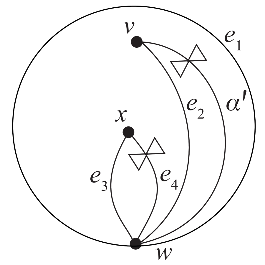
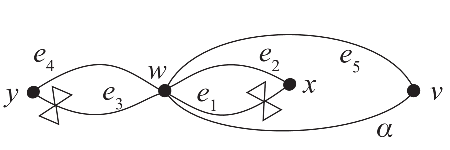
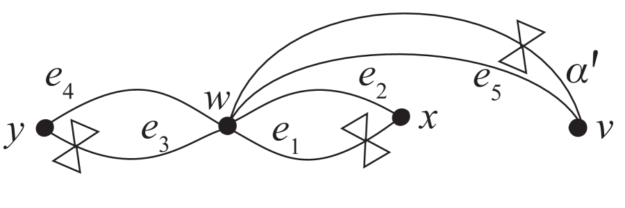
Again by compatibility, we denote the tagging of any arc ending at , , and by , , and , respectively. Also, exactly one of and is notched at . Thus , , and .
In , application of a skein relation implies , where is the envelope of the dangle (Definition 3.8). Lemma 2.5 further shows , and since the underlying curves of and are the same, in fact . It follows that
Case 5. The arc is one of two common edges of two puzzle pieces of type A and B.
Figure 4.4 shows the two puzzle pieces glued along .
Note that and have different tags at , and and have different tags at . The puncture-skein relation and Lemma 2.5 imply that . Since , it follows that
Case 6. The arc is the common edge of two puzzle pieces of type A and C.
Figure 4.5 shows the two puzzle pieces. Similarly to the previous cases,
Case 7. The arc is the common edge of two puzzle pieces of type B.
There are two possibilities. The first one is identical to the right figure in Figure 4.5, but where plays the role of . The exchange relation is the same as in Case 6, since the cluster mutation is involutive. Thus the argument from Case 6 applies in this case.
The second possibility is the one shown in Figure 4.6. Then
Case 8. The arc is one of two common edges of two puzzle pieces of type B.
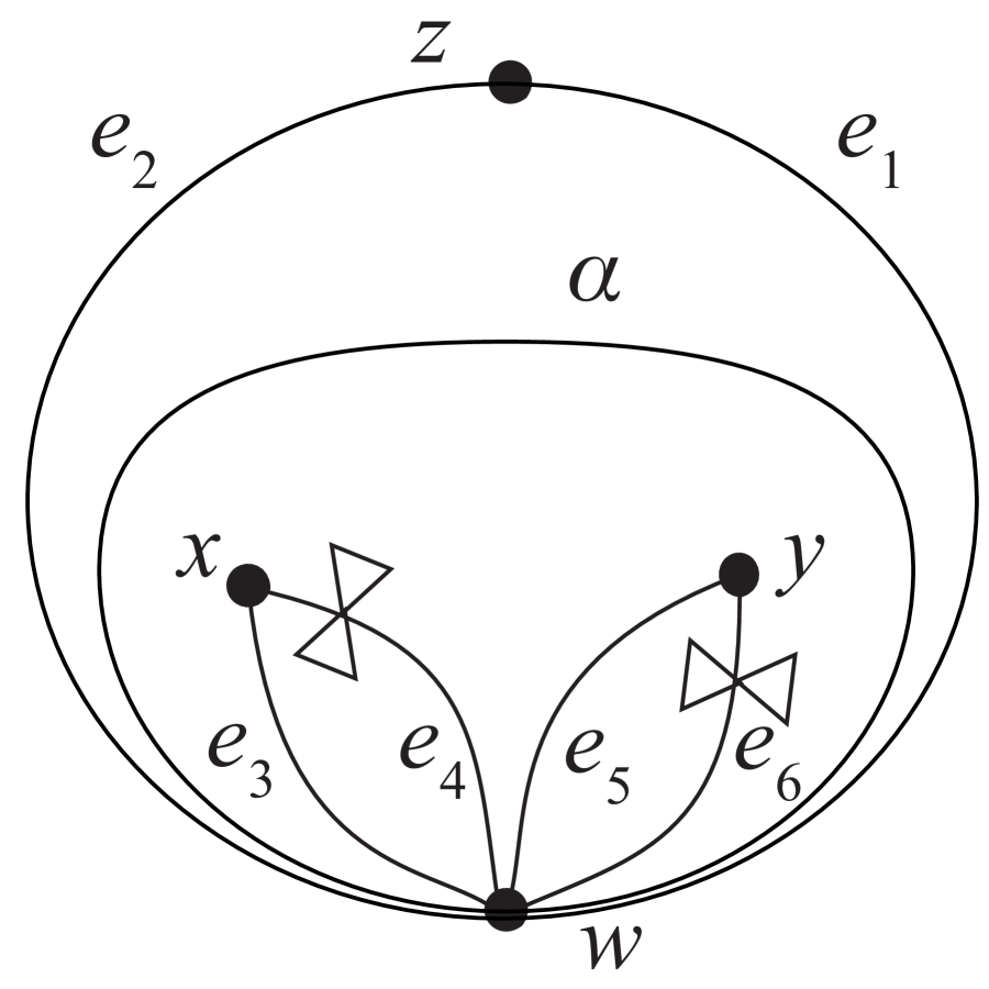
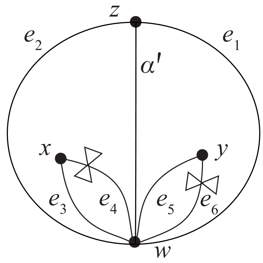
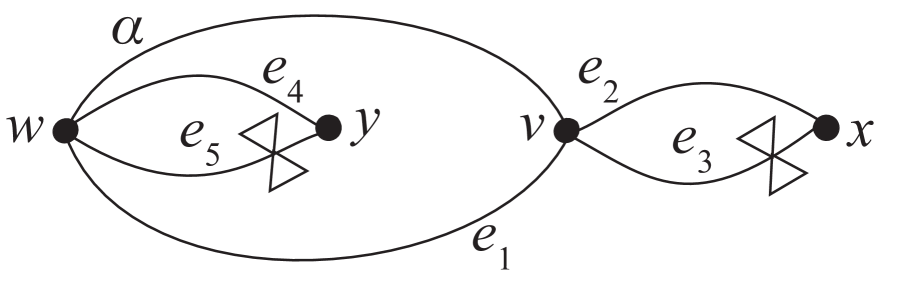
Two puzzle pieces glue together to produce a triangulation for . We distinguish between two subcases, as depicted in Figures 4.7 and 4.8.
In subcase I shown in Figure 4.7, we have
Note that because it is on . In subcase II shown in Figure 4.8, we have
Case 9. The arc is the common edge of two puzzle pieces of type B and C.
See Figure 4.9. We have
Case 10. The arc is the common edge of two puzzle pieces of type C.
In this situation, the surface must be . See Figure 4.10. Then
Step 2. Suppose that is on a dangle.
Any dangle must be contained inside one of the tagged puzzle pieces in Figure 3.4. Suppose first that is notched at the jewel. The mutation of in a puzzle of type B is the inverse of the flip described in Case 2 and Figure 4.2 (and in Figure 4.2 plays the role of ). Since the mutation is an involution, the compatibility follows from Case 2. In the case of a puzzle of type C, the mutation is the inverse of the flip in Case 5 and Figure 4.4. In the case of type D, it is the inverse of the flip in subcase I of Case 8 and Figure 4.7. This takes care of all situations where is on a dangle. If is tagged plainly at the jewel, then the only difference is that, in the flipped diagram, one needs to change the tagging at the vertex which was the jewel. The rest of the computation is identical. ∎
Remark 4.4.
By tensoring a commutative ring , we obtain
We complete the proof of Compatibility Lemma by showing that is injective. Indeed, we will show that for any integral domain , in Remark 4.4 is injective.
Roger-Yang’s homomorphism will factor in our proofs coming up. We here present a slightly different version that we find easier to apply. See [MW21, Section 3] for details.
Lemma 4.5.
Let be an integral domain. Suppose is an ideal triangulation of , and let denote its set of edges. Then there is a well-defined homomorphism , where is the field of fraction of .
Proof.
We first consider case. The map sends each arc in to the function on the decorated Teichmüller space that gives the lambda-length of . It follows by [MW21, Lemma 3.3] that factors through . By tensoring a general integral domain , we obtain a similar map .
The decorated Teichmüller space is homeomorphic to and the homeomorphism maps each decorated hyperbolic metric to the lambda-lengths of [Pen87, Theorem 3.1]. Thus, is a Zariski-dense semialgebraic set in an -dimensional complex torus . Therefore, is a set of algebraically independent elements. Hence there is a well-defined, canonical isomorphism that maps to . By tensoring , we obtain . Then composition of and followed by the canonical inclusion yields . ∎
Proposition 4.6.
Let be an integral domain. The algebra homomorphism is injective.
Proof.
We fix an ordinary triangulation on . Let be the set of edges in . There is a commutative diagram
Here is the natural inclusion of the cluster algebra into its field of fraction, and is the homomorphism in Remark 4.4. The map is the Roger-Yang homomorphism from Lemma 4.5. For each , we have . It follows that , since all of the elements of can be written as a Laurent polynomial with respect to the cluster variables in a fixed cluster. Since is injective, must also be injective. ∎
5. Integrality of and its implications
This section is mainly devoted to a proof of integrality of using the injective homomorphism and techniques from algebraic geometry, in particular dimension theory. For the definition and basic properties of the dimension of algebraic varieties, see [Eis95, Section 8]. We will need the following lemma from commutative algebra.
Let be a field and let be a -algebra, which is an integral domain. The (Krull) dimension of is the maximal length of the strictly increasing chain of prime ideals of . For the associated affine scheme , its dimension is defined as .
Lemma 5.1.
Let be a field and let be a -algebra, which is an integral domain. Let be its field of fractions. Suppose that the transcendental degree of is . Then .
Proof.
When is a finitely generated algebra, the statement is well known [Eis95, Theorem A, p.221]. We assume that is not finitely generated.
Take a chain of prime ideals of . For each , pick . Let be the subalgebra of generated by , and be its field of fractions. Since is a finitely generated algebra, .
On the other hand, if we set , the sequence is an increasing sequence of prime ideals, and it is strictly increasing as . Therefore, , so we have . This is valid for arbitrary increasing chains of prime ideals, we obtain the desired result. ∎
We are now ready for the proof of integrality.
Theorem 5.2.
Suppose that and . Then is an integral domain.
Proof.
To start, assume that is not a -puncture sphere, so that is defined. As before, we fix an ordinary ideal triangulation on , and let denote the edges of the triangulation.
By [MW21, Lemma 3.2], every element in can be written as a rational function (indeed a Laurent polynomial) with respect to the edge classes in . In particular, for any , there is a rational function with respect to , such that . Indeed, the numerator is not a zero polynomial, because it is given by the trace of a product of matrices whose coefficients are edge classes [RY14, Theorem 3.22]. Then we can construct a ring extension and an extended homomorphism , which maps . Since , is also a subring of . We may repeat this procedure and extend the algebra further, until the extended map is surjective. Since is a finitely generated algebra (Theorem 2.8), this procedure is terminated in finitely many steps. Therefore, we obtain a ring extension of in and a surjective homomorphism .
Combined with the Roger-Yang homomorphism from Lemma 4.5 (with -coefficient), we have the commutative diagram
Note that is an integral domain, as it is a subring of . So is . So the associated affine scheme is integral (irreducible and reduced). If we denote the number of edges in by , then the transcendental degree is . Since the field of fractions of is also , by Lemma 5.1, .
Since is a surjective homomorphism, so is . If we denote , then . Then is a closed subscheme of , defined by the ideal . Thus
and if is nontrivial, then .
Recall from the proof of Lemma 4.5 that is a composition of the map . Every element in can be written as a Laurent polynomial with respect to [MW21, Lemma 3.2], so if we denote by the multiplicative set of monomials with respect to , then there is a localized morphism , which turns out to be an isomorphism [MW21, Lemma 3.4]. The localization of a ring corresponds to taking an open subset of the associated scheme. Thus has a (Zariski) open subset . In particular, has an irreducible component, which has an open dense subset isomorphic to the algebraic torus of dimension . Therefore, .
The only possibility is and is the trivial ideal. Therefore and hence is an integral domain. Since has no torsion (Remark 2.3), and it is also an integral domain.
Now the only remaining case is where is undefined. But we may formally set and define as (see Theorem 2.9 for the notation). Then we can follow the same line of the proof to get the same conclusion. ∎
Remark 5.3.
If (so and ), is no longer an integral domain [ACDHM21, Remark 6.3].
Theorem 5.4.
Suppose that and . Then is a non-commutative domain.
Remark 5.5.
Proofs of Theorem A and Theorem B.
Theorem A of [MW21] states that if is an integral domain, must be injective. Thus, we obtain Theorem A. In the last part of the proof of 5.2, we showed that , so they have the same field of fractions. Since is an algebraic extension of in its field of fractions, they have the same field of fractions, too. Thus, we can conclude that can be understood as a deformation quantization of . ∎
6. Implications for
The compatibility of the curve algebra and cluster algebra provides us new insight to some questions on the structure of cluster algebras. In this section, we investigate two questions regarding the finite generation of (Theorem C) and the comparison of with (Theorem D). We still assume that .
6.1. Non-finite generation for
It was observed in [Lad13, Proposition 1.3], following [Mul13, Proposition 11.3], that is not finitely generated for all . It is plausible to believe that is more complicated than . Thus one may guess that is not finitely generated for all . However, the lack of a functorial morphism makes it difficult to prove the non-finite generation of in general. We suggest a new approach to resolve this issue, using invariant theory and ‘mod 2 reduction.’
The first key technical ingredient is Nagata’s theorem [Dol03, Theorem 3.3] and its extension to arbitrary base ring by Seshadri [Ses77]. For a finitely generated -algebra , it is not true that its subalgebra is finitely generated. However, if is equipped with a reductive group -action, Nagata’s theorem tells us that the invariant subalgebra is finitely generated. For our purpose, the following consequence of the Seshadri-Nagata’s theorem is handy.
Lemma 6.1.
Let be a field. Let be a finitely generated -graded -algebra, so such that . Then is finitely generated.
Proof.
Recall that an affine group scheme -action on is given by a -linear map
which makes as a comodule under the coalgebra . We may set
Then it is straightforward to check that the above coalgebra strucure is equivalent to a -grading structure on . Now , which is finitely generated by [Ses77, Remark 4, p.242]. ∎
Remark 6.2.
The group action in the proof of Lemma 6.1 should be understood as an affine group scheme action, not a set-theoretic one. We will consider the case. But then the set of -valued points of has only one point . Thus, set-theoretically, it is a trivial group.
Remark 6.3.
Primarily, we will use the contrapositive of Lemma 6.1. If is not finitely generated, then is not finitely generated.
Proposition 6.4.
Let be an integral domain. Then and have -graded ring structure.
Proof.
We may impose as a -graded algebra structure in the following way. Let be the vertex set. For an arc connecting and another vertex (we allow ), the grade of is defined as , where is the standard basis of . For any loop, its grade is . Finally, the grade of the vertex class is (hence the grade of is ). It is straightfoward to check that all skein relations in Definition 2.1 are homogeneous. Thus, it is well-defined.
Since is generated by homogeneous elements, is also a -graded algebra. ∎
Remark 6.5.
For each vertex , we may impose a -graded algebra structure on (and on ), by composing the grade map with the -th projection .
The following proposition is proved by Ladkani in [Lad13, Proposition 1.3], over coefficients. The same proof works for arbitrary base ring, but we provide a sketch for the sake of completeness.
Proposition 6.6 (Ladkani).
For any integral domain and , is not finitely generated.
Proof.
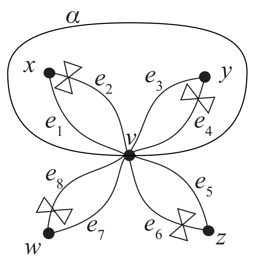
By definition when , is generated by ordinary arcs only, and all exchange relations are homogeneous of degree two with respect to the -grading in Proposition 6.4. Therefore, a cluster variable cannot be expressed as a polynomial with respect to the other cluster variables. On the other hand, there are infinitely many non-isotopic arc classes on , so there are infinitely many cluster variables. Thus, cannot be finitely generated. ∎
Over -coefficient, we may reduce the proof of the non-finite generation to case.
Proposition 6.7.
Let . If is not finitely generated, then is not finitely generated.
Proof.
We think of as a subalgebra of . Thus, instead of arcs and tagged arcs, we will describe all elements as a combination of arcs and vertices.
We construct a morphism between curve algebras induced from which forgets a vertex . With respect to , note that and have a -graded structure (Remark 6.5). Let be the grade 0 subalgebra of .
We claim that when , there is a well-defined surjective homomorphism . Indeed, is generated by the following elements:
-
(1)
vertex classes (except );
-
(2)
loop classes;
-
(3)
tagged arcs disjoint from ;
-
(4)
where each are arcs connecting with other vertices;
-
(5)
where is an arc connecting and itself.
For each case, by applying a puncture-skein relation, we can find a representative which is disjoint from . For (1), (2), and (3), this is clear. For (4), by the puncture-skein relation, we can resolve the crossing of to get the sum of two arcs disjoint from , which we call and . Now if we forget , then as isotopy classes on , we have . Thus . The case of (5) is similar. Since we only used the puncture-skein relation, the map is well-defined. The surjectivity is immediate.
By composition, we obtain a map
The cluster algebra is generated by multiples of tagges arcs, and the image of them by the map is still a multiple of tagged arcs on . The only exception is a multiple of , where is an arc whose both ends are . (Note that two ends of , whose underlying curve is , must be tagged in the same way, so or .) In this case, after applying the puncture-skein relation at the endpoint of , becomes a multiple of the sum of two loops and . Once we forget the vertex, then in we have . In summary, the image of by is still tagged arcs on . Therefore, if , the image is in , and we have a morphism .
It is straightforward to check that is surjective. Therefore, if is not finitely generated, then is not finitely generated. By Lemma 6.1, is not finitely generated, too. ∎
Remark 6.8.
On the other hand, when , is generated by ordinary arcs only. Thus does not factor through in general.
Remark 6.9.
The reduction map does not behave well for a general base ring . For example, both the punctured loop around and a trivial loop near both map to the same trivial loop under the map that forgets . Thus but after the forgetful map . In particular, if the base ring is a field of characteristic , is a zero map.
Proof of Theorem C for .
Step 1. First of all, observe that to show the non-finite generation of , it is sufficient to show that is not finitely generated, as there is a surjective morphism .
Step 2. Let be a subalgebra generated by arcs, loops, and vertices, but not the inverses of vertices. By Definition 4.1, we know that the homomorphism indeed factors through . By taking the tensor product with , we obtain a homomorphism
We have a similar variation for the map .
Step 3. We specialize to . For the vertex that is forgotten by , we impose the associated -grading structure on , , and on (Remark 6.5). Consider the composition
and denote it by .
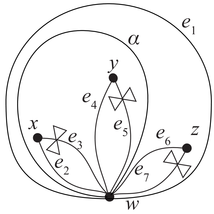
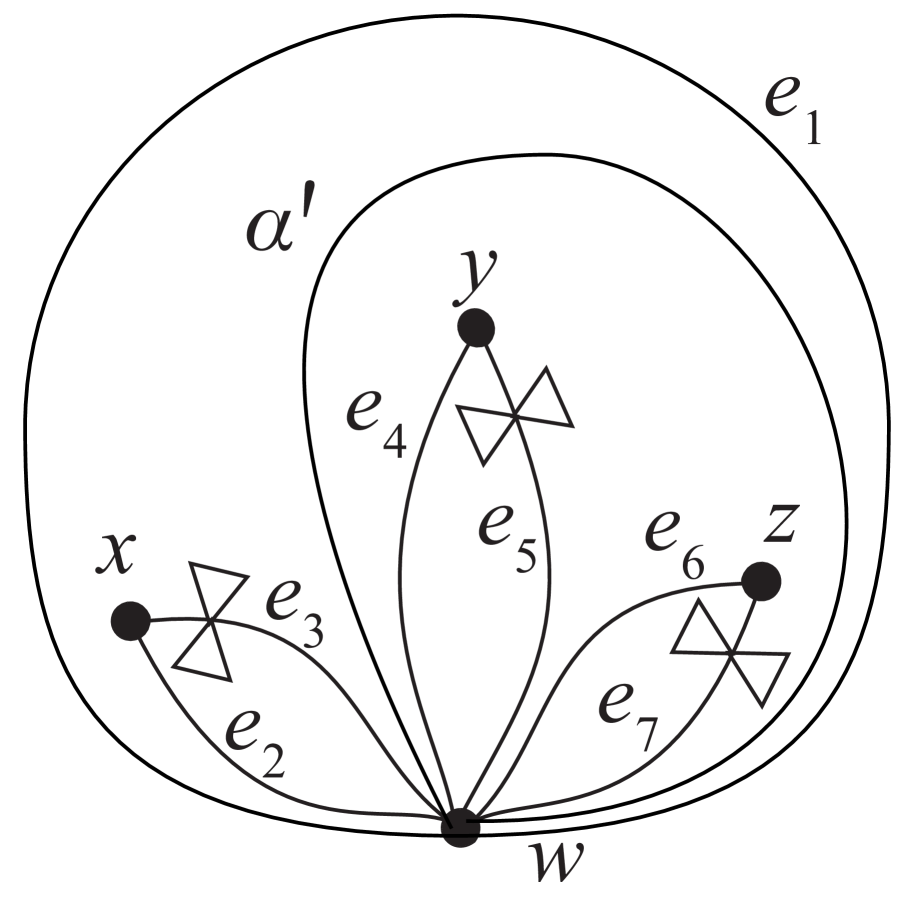
We claim that the image of is . Indeed, if we denote the unique vertex by , then the image of is generated by and for an ordinary arc . Applying the puncture-skein relation, we have for two loops. But any loop in is a -torus knot for two relatively prime integers and , and because they are realized by the same . Thus, and so is . Therefore, the image of is generated by ordinary arcs only, so is not finitely generated by Proposition 6.6. Therefore, and are not finitely generated by Lemma 6.1. By Proposition 6.7, for all are not finitely generated.
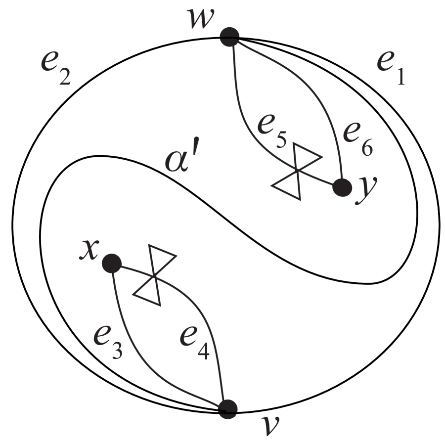
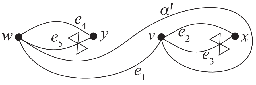
Step 4. Now we consider . Recall that there is a to one branched covering , branched at two points. This induces a covering map that sends two puctures to the corresponding two punctures. by taking the image of every curve class, we obtain a map , which is clearly surjective. This map induces a surjective map . Since is not finitely generated and is surjective, is also not finitely generated. Applying Proposition 6.7, we get the desired result. ∎
Remark 6.10.
Another way to think about the special property of is the following. For a fixed triangulation , one may write the vertex class as a Laurent polynomial with respect to the edges in . An explicit formula can be found, for example, in [MSW11, Definition 5.2]. is the only case that is a multiple of two.
6.2. Finite generation for
The situation is entirely different when . The finite generation of follows immediately from the presentation of in Theorem 2.9.
Proof of Theorem C for .
The proof is essentially identical to that of [ACDHM21, Prop 3.2], but for the reader’s convenience, we sketch the proof here.
Recall that, without loss of generality, we assume that the punctures lie on a small circle , and is the simple arc connecting and in the disk bounded by .
Let be a tagged arc. So connects two (not necessarily different) punctures. If is inside of , then is isotopic to one of (if connects two distinct vertices) or (if two ends of are the same). So is either zero or one of , , , or , depending on the tagging.
If is outside of , then we can ‘drag into’ and use the puncture-skein relation to break the curve at the vertices. Then we can describe as a combination of tagged arcs which meet the outside smaller number of times. Now we may apply induction and get the desired result. ∎
We believe that by the virtue of Theorem 2.9, the following is an interesting and approachable problem.
Question 6.11.
Find a presentation of .
6.3. Comparison with the upper cluster algebra
We finish this paper with some remarks on the upper cluster algebra . Recall that is the subalgebra of generated by isotopy classes of loops, arcs and decorated arcs (Definition 2.10).
Lemma 6.12.
There are inclusions of algebras
Proof.
The Compatibility Lemma and the fact that the image of factor through imply the first inclusion. There are two extra classes of generators of in : loop classes and , where is an arc class with two ends both at . (Note that and are in , if .) We obtain that is a sum of two loop classes by applying the puncture-skein relation. For an ordinary triangulation with edge set , it has been proven several times ([FG06, Section 12], [MW13, Theorem 4.2], and [RY14, Theorem 3.22]) that a loop class is a Laurent polynomial with respect to the edges in a triangulation. The case of a tagged triangulation is reduced to the case of an ordinary triangulation, by [MSW11, Proposition 3.15]. Thus, we conclude that any element in can be written as a Laurent polynomial with respect to the edges in a fixed tagged ideal triangulation.
If we show that this expression is unique, then set theoretically, and we are done. This is because the three rings in the statement share isomorphic field of fractions. For a nonzero element , if there are two Laurent polynomial expressions and for , then provides an algebraic relation in their field of fractions generated by edge classes in a fixed triangulation. Since their field of fractions are purely transcendentally generated by edge classes, this is impossible. ∎
Proof of Theorem D.
Remark 6.13.
Remark 6.14.
If , is not a subalgebra of , because of the vertex classes. For a fixed ordinary triangulation and its edge set , a vertex class can be written as a Laurent polynomial with respect to (see the proof of [MW21, Lemma 3.2]). However, this is no longer true for a tagged triangulation . On the other hand, when , we do not consider a tagged triangulation, so and hence .
Remark 6.15.
In a recent breakthrough in [GHKK18], for each combinatorial data defining a cluster algebra, Gross, Hacking, Keel, and Kontsevich defined yet another algebra motivated from mirror symmetry, the so-called mid-cluster algebra ( in their terminology). For , the mid-algebra is indeed equal to and it admits a canonical basis parametrized by the tropical points of the dual cluster variety ([MQ23, Theorem 1.3], [FG06, Section 12]).
To the authors’ knowledge, it has not been rigorously proved whether or not.
Conjecture 6.16.
-
(1)
.
-
(2)
If , . In particular, if , .
References
- [AB20] D. Allegretti and T. Bridgeland. The monodromy of meromorphic projective structures. Trans. Amer. Math. Soc. 373 (2020), no. 9, 6321–6367.
- [ACDHM21] F. Azad, Z. Chen, M. Dreyer, R. Horowitz, and H.-B. Moon. Presentations of the Roger-Yang generalized skein algebra. Algebr. Geom. Topol., 21 (2021), no. 6, 3199–3220.
- [BMS22] V. Bazier-Matte and R. Schiffler. Knot theory and cluster algebras. Adv. Math. 408 (2022), Paper No. 108609, 45 pp.
- [BMRS15] A. Benito, G. Muller, Greg, J. Rajchgot, and K. Smith. Singularities of locally acyclic cluster algebras. Algebra Number Theory 9 (2015), no. 4, 913–936.
- [BZ05] A. Berenstein and A. Zelevinsky. Quantum cluster algebras. Adv. Math. 195 (2005), no. 2, 405–455.
- [BHMV95] C. Blanchet, N. Habegger, G. Masbaum, and P. Vogel. Topological quantum field theories derived from the Kauffman bracket. Topology 34 (1995), no.4, 883–927.
- [BKL23] W. Bloomquist, H. Karuo, and T. Le. Degeneration of skein algebras and quantum traces. preprint. arXiv:2308.16702.
- [BKPW16a] M. Bobb, S. Kennedy, H. Wong, and D. Peifer. Roger and Yang’s Kauffman bracket arc algebra is finitely generated. J. Knot Theory Ramifications 25 (2016), no. 6, 1650034, 14 pp.
- [BKPW16b] M. Bobb, D. Peifer, S. Kennedy, and H. Wong. Presentations of Roger and Yang’s Kauffman bracket arc algebra. Involve 9 (2016), no. 4, 689–698.
- [Bul97] D. Bullock. Rings of -characters and the Kauffman bracket skein module Commentarii Mathematici Helvetici 72 (1997), no. 4, 521–542.
- [BFKB99] D. Bullock, C. Frohman, and J. Kania-Bartoszyńska. Understanding the Kauffman bracket skein module. J. Knot Theory Ramifications 8 (1999), no. 3, 265–277.
- [CLS15] I. Canakci, K. Lee, R. Schiffler. On cluster algebras from unpunctured surfaces with one marked point. Proc. Amer. Math. Soc. Ser. B 2 (2015), 35–49.
- [Dol03] I. Dolgachev. Lectures on invariant theory. London Mathematical Society Lecture Note Series, 296. Cambridge University Press, Cambridge, 2003. xvi+220 pp.
- [Eis95] D. Eisenbud. Commutative algebra. With a view toward algebraic geometry. Graduate Texts in Mathematics, 150. Springer-Verlag, New York, 1995. xvi+785 pp.
- [FG06] V. Fock and A. Goncharov. Moduli spaces of local systems and higher Teichmüller theory. Publ. Math. Inst. Hautes Études Sci. 103 (2006), 1–211.
- [FST08] S. Fomin, M. Shapiro, and D. Thurston. Cluster algebras and triangulated surfaces. I. Cluster complexes. Acta Math. 201 (2008), no. 1, 83–146.
- [FT18] S. Fomin and D. Thurston. Cluster algebras and triangulated surfaces Part II: Lambda lengths Mem. Amer. Math. Soc. 255 (2018), no. 1223, v+97 pp.
- [FZ02] S. Fomin and A. Zelevinsky. Cluster algebras. I. Foundations. J. Amer. Math. Soc. 15 (2002), no. 2, 497–529.
- [GSV05] M. Gekhtman, M. Shapiro, and A. Vainshtein. Cluster algebras and Weil-Petersson forms. Duke Mathematical Journal, 127 (2005), no. 2, 291–311.
- [GHKK18] M. Gross, P. Hacking, S. Keel, and M. Kontsevich. Canonical bases for cluster algebras. J. Amer. Math. Soc. 31 (2018), no. 2, 497–608.
- [HI15] K. Hikami and R. Inoue. Braids, complex volume and cluster algebras. Algebr. Geom. Topol. 15 (2015), no. 4, 2175–2194.
- [IOS23] T. Ishibashi, H. Oya, L. Shen. for cluster algebras from moduli spaces of -local systems. Adv. Math. 431 (2023), Paper No. 109256, 50 pp.
- [Jon85] V.F.R. Jones. A new polynomial invariant for links via von Neumann algebras. Bull. Amer. Math. Soc 12 (1985), 103–122.
- [Lad13] S. Ladkani. On cluster algebras from once punctured closed surfaces. preprint, arXiv:1310:4454.
- [LS19] K. Lee and R. Schiffler. Cluster algebras and Jones polynomials. Selecta Math. (N.S.) 25 (2019), no. 4, Paper No. 58, 41 pp.
- [MQ23] T. Mandel and F. Qin. Bracelets bases are theta bases. preprint. arXiv:2301.11101.
- [Mon09] G. Mondello. Triangulated Riemann surfaces with boundary and the Weil-Petersson Poisson structure. J. Differential Geom. 81 (2009), no. 2, 391–436.
- [MW21] H.-B. Moon and H. Wong. The Roger-Yang skein algebra and the decorated Teichmüller space. Quantum Topol. 12 (2021), no. 2, 265–308.
- [Mul13] G. Muller. Locally acyclic cluster algebras. Adv. Math. 233 (2013), 207–247.
- [Mul16] G. Muller. Skein and cluster algebras of marked surfaces. Quantum Topol. 7 (2016), no. 3, 435–503.
- [MSW11] G. Musiker, R. Schiffler, and L. Williams. Positivity for cluster algebras from surfaces. Adv. Math. 227 (2011), no. 6, 2241–2308.
- [MW13] G. Musiker and L. Williams. Matrix formulae and skein relations for cluster algebras from surfaces. Int. Math. Res. Not. IMRN 2013, no. 13, 2891–2944.
- [NT20] W. Nagai and Y. Terashima. Cluster variables, ancestral triangles and Alexander polynomials. Adv. Math. 363 (2020), 106965, 37 pp.
- [Pen87] R. C. Penner. The decorated Teichmüller space of punctured surfaces. Comm. Math. Phys. 113 (1987), 299–339.
- [Pen92] R. C. Penner. Weil-Petersson volumes. J. Differential Geom. 35 (1992), no. 3, 559–608.
- [Prz91] J. Przytycki. Skein modules of 3-manifolds. Bull. Polish Acad. Sci. Math. 39 (1991), no. 1-2, 91–100.
- [PS00] J. H. Przytycki and A. Sikora. On skein algebras and -character varieties. Topology 39 (2000), no. 1, 115–148.
- [RT91] N. Reshetikhin and V.G. Turaev. Invariants of -manifolds via link polynomials and quantum groups. Invent. Math. 103 (1991), no. 3, 547–597.
- [RY14] J. Roger and T. Yang. The skein algebra of arcs and links and the decorated Teichmüller space. J. Differential Geom. 96 (2014), no. 1, 95–140.
- [Ses77] C. S. Seshadri. Geometric reductivity over arbitrary base. Advances in Math. 26 (1977), no. 3, 225–274.
- [Tur91] V. G. Turaev. Skein quantization of Poisson algebras of loops on surfaces. Ann. Sci. École Norm. Sup. (4), 24(6):635–704, 1991.
- [Wit89] E. Witten. Quantum field theory and the Jones polynomial Comm. Math. Phys. 121 (1989), no. 3, 351–399.
- [Yac19] M. Yacavone. Cluster algebras and the HOMFLY polynomial. preprint. arXiv:1910.10267.