General approach to function approximation

Abstract

Having a function $f$ and a set of functionals $\{\mathcal{C}_{n}\}$, $c_{n}^{f}\equiv\mathcal{C}_{n}\left(f\right)$, one can interpret function approximation very generally as a construction of some function $\mathcal{A}^{f}$ such that $c_{n}^{f}=\mathcal{C}_{n}\left(\mathcal{A}^{f}\right)$. All known approximations can be interpreted in this way and we review some of them. In addition, we construct several new expansion types including three rational approximations.

Keywords: functional action, characteristic number matching, rational approximation.

MSC classification: 41-02, 41A58, 41A20.

1 Introduction

Applications of function approximations are countless: evaluation of functions on computers, transformation of functions into a form suited for further processing (integration, differentiation), frequency analysis, (approximate) solutions of differential equations, etc. A natural point of view which is common to all approximation methods is that by an approximation of a function $f$ one can understand another function $\mathcal{A}^{f}$ which meets a number of constraints (conditions) true for $f$. $\mathcal{A}^{f}$ is usually constructed such as to keep some well defined function form and the constraints are met by adjusting coefficients appearing within this form. The number of constraints can be finite or infinite, and in most cases the degree of the approximation can be increased by increasing the number of conditions which are obeyed. For an exact approximation $\mathcal{A}^{f}=f$ to be achieved, one in general expects an infinite number of fulfilled constraints as a necessary (but often not sufficient) condition. This can be formalized in a framework where requirements are represented by numbers resulting from the action of some predefined set of functionals on $f$. Then the construction of an approximation corresponds to tuning the above-mentioned coefficients, such as to reproduce these numbers by $\mathcal{A}^{f}$. As an example we can mention the Taylor series which are based on matching the derivatives by power series, or the Fourier expansion which can be seen as matching the integrals where the integrand is $f\left(x\right)$ multiplied by $\sin\left(nx\right)$ or $\cos\left(nx\right)$.

These ideas are not new, similar ideas have been presented in [1, 2, 3, 4, 5]. To justify our work we bring forward two points to make a distinction.

• First point is conceptual: all previous works are based on linear functionals. The idea of linearity is indeed attractive when practical considerations are taken into account, but is not necessary to define the concept of approximation. Functionals need to constrain the function in the first place, not to act linearly. We thus extend the definition of approximation in this direction and provide a simple example of this (i.e. non-linear) type.

• The second point is practical: we construct several new expansions not present in other works.

The introduced notion of an approximation does not imply the convergence (of any type) of $\mathcal{A}^{f}$ to $f$. In most of this text we focus only on the approximation properties and not on the convergence ones. We do this because (inferring from the existing approximations) the convergence questions are usually technically complicated and their study (weakness/strength, sufficiency/necessity, bounding strategies, etc.) often represents a large topic which would exceed the intended extent of this text, where many different approximation types are mentioned.

Also, our text does not rely on proving a single main idea or theorem. Going through various function approximations a couple of proofs are presented labeled as propositions.

In Sec. 2 we introduce the notion of an approximation more formally and discuss some basic properties. The section which follows then reviews some of the existing examples and shows how to interpret them in the general approximation approach. We present new function expansions in Sec. 4 and close the text by summary, conclusion and outlook.

2 General approach to function approximation

2.1 Definitions

Let $f\left(x\right)$ be a real-valued function defined on some (open or closed) interval $\left(a,b\right)\subset\overline{\mathbb{R}}$ and let $\left\{\mathcal{C}_{n}\right\}_{n=0}^{\infty}$ be a sequence of real functionals acting on $f$

$$\mathcal{\mathcal{C}}_{n}:f_{\left(a,b\right)}\left(x\right)\rightarrow\mathbb{R}.$$

By characteristic numbers of the function $f$ we will understand the sequence of real numbers $\left\{c_{n}^{f}\right\}_{n=0}^{\infty}$ defined by

$$c_{n}^{f}\equiv\mathcal{C}_{n}\left(f\right).$$

By a partial approximation of the function $f$ of the order $N$ we will understand any function $\mathcal{A}_{N}^{f}\left(x\right)$ for which the action of $\mathcal{\mathcal{C}}_{n}$ is defined for all $n\leq N$ having the property

$$\mathcal{\mathcal{C}}_{n}\left(\mathcal{A}_{N}^{f}\right)=c_{n}^{f}\text{ for all }n\leq N.$$

A function $\mathcal{A}^{f}\left(x\right)\equiv\mathcal{A}_{\infty}^{f}\left(x\right)$ will be called the approximation of the function $f$.

2.2 Properties of functionals and approximations

Intuitively, some basic properties of functionals are expected. We call the functional $\mathcal{\mathcal{C}}_{i}\,\in\,\mathcal{C}\equiv\left\{\mathcal{C}_{n}\right\}_{n=0}^{\infty}$ dependent on $\mathcal{C}\backslash\mathcal{\mathcal{C}}_{i}$ if for any $f$ (for which the functionals are well defined) $c_{i}^{f}$ can be expressed as a function of the remaining characteristic numbers

$$c_{i}^{f}=c_{i}^{f}\left(c_{0}^{f},\ldots,c_{i-1}^{f},c_{i+1}^{f},\ldots\right).$$

For the set $\mathcal{C}$ to be rich enough to permit an approximation of an interestingly large family of functions, one expects it to contain an infinite number of independent functionals. For aesthetic reasons one may prefer all functionals in $\mathcal{C}$ to be independent.

Also, in situations where the functional action needs to be distributed over infinite sums, the functionals are assumed to be continuous. Yet, because our approach is very general, we prefer to assume that the various operations we perform are valid, i.e. that the appearing objects have the necessary properties (whatever these are), rather then specifying conditions for them.

2.2.1 Linearity

Most of the actually used approximations are based on linear functionals, i.e. one has

$$\mathcal{C}_{n}\left(f+\alpha g\right)=\mathcal{C}_{n}\left(f\right)+\alpha\mathcal{C}_{n}\left(g\right)\text{ for all }f,g\text{ and }n\,\in\,\mathbb{N}_{0},\,\alpha\,\in\,\mathbb{R}.$$

Such approximations are very appealing if a set of functions $\left\{\Delta_{n}\right\}_{n=0}^{\infty}$ with the delta property

$$\mathcal{C}_{n}\left(\Delta_{m}\right)=\delta_{n,m}$$ (1)

exists. When so, an approximation of $f$ can be easily constructed in the form of an infinite sum

$$\mathcal{A}^{f}\left(x\right)=\sum_{m=0}^{\infty}c_{m}^{f}\Delta_{m}\left(x\right),$$ (2)

where the existence of the limit is assumed. Assuming further that the action of $\mathcal{\mathcal{C}}_{i}$ can be distributed over this infinite sum, one observes that the expression (2) indeed reproduces the characteristic numbers of $f$

$$\mathcal{C}_{n}\left(\mathcal{A}^{f}\right)=\sum_{m=0}^{\infty}c_{m}^{f}\mathcal{C}_{n}\left(\Delta_{m}\right)=\sum_{m=0}^{\infty}c_{m}^{f}\delta_{n,m}=c_{n}^{f}.$$

In this text we will refer to $\Delta_{n}$ using the term “delta function”.

Another interesting scenario, which also appears in practice, is represented by the set of functions $\left\{\nabla_{n}\right\}_{n=0}^{\infty}$ with the property

$$c_{n}^{\nabla_{m}}\equiv\mathcal{C}_{n}\left(\nabla_{m}\right)=0\text{ for all }n<m.$$ (3)

Also in this case one can propose to build an approximation as a series with multiplicative coefficients (supposing it is well defined)

$$\mathcal{A}^{f}\left(x\right)=\sum_{m=0}^{\infty}t_{m}\nabla_{m}\left(x\right),$$ (4)

where the question of $t_{m}$ values arises. Assuming the distribution of the functional action is justified, one has

$$\mathcal{C}_{n}\left(\mathcal{A}^{f}\right)=\sum_{m=0}^{\infty}t_{m}\mathcal{C}_{n}\left(\nabla_{m}\right)=\sum_{m=0}^{n}t_{m}c_{n}^{\nabla_{m}}\overset{!}{=}c_{n}^{f},$$

where the notation $\overset{!}{=}$ reads “should be equal to”. The relation between $t_{m}$ and $c_{n}^{f}$ is therefore represented by an infinite triangular matrix

$$\boldsymbol{c^{f}}=\boldsymbol{Tt},\quad\boldsymbol{T}=\left(\begin{array}[]{cccc}c_{0}^{\nabla_{0}}&0&0&\ldots\\ c_{1}^{\nabla_{0}}&c_{1}^{\nabla_{1}}&0&\ldots\\ c_{2}^{\nabla_{0}}&c_{2}^{\nabla_{1}}&c_{2}^{\nabla_{2}}&\ldots\\ \vdots&\vdots&\vdots&\ddots\end{array}\right),$$

which can be easily inverted in practice (and sometimes also formally) $\boldsymbol{t}=\left(\boldsymbol{T}\right)^{-1}\boldsymbol{c^{f}}$, thus allowing for an easy-to-achieve approximation. We will refer to $\nabla_{n}$ using the term “triangular function”.

An additional issue, which can be addressed when series of delta functions are used, is the behavior of the latter with the number of matched constraints increasing to infinity. Here we naturally extend the definition of a delta function to partial approximations by

$$\mathcal{C}_{n}\left(\Delta_{m}^{[N]}\right)=\delta_{n,m}\text{ for }n,m\leq N,$$ (5)

where $[N]$ indicates the approximation order. If functions $\Delta_{m}$ exist then they also represent partial delta functions, i.e. $\Delta_{m}^{[N]}$ exist too. However, since $\Delta_{m}^{[N]}$ functions need to satisfy only a finite number of conditions (i.e. conditions for their existence are weaker) one can observe situations

• where $\Delta_{m}^{[N]}$ exist, but $\Delta_{m}$ do not, or

• where, for fixed $N$, several realizations of $\Delta_{m}^{[N]}$ exist, with $\Delta_{m}$ being one of them.

Similarly one can define partial triangular functions by

$$\mathcal{C}_{n}\left(\nabla_{m}^{[N]}\right)=0\text{ for all }n<m\leq N$$

and address analogous questions.

2.2.2 Construction of approximations

One can think of multiple ways of how an approximation can be built. It is natural to expect from its function form to have some generality, i.e. to be suitable for approximating various functions, while keeping its form. Thus one intuitively comes to the following ideas:

• The form of an (partial) approximation has some well defined logical structure, which remains the same for all approximated functions.

• The (partial) approximation is achieved by varying coefficients $a_{i}$ appearing within this fixed form.

Here, once more, some general properties are expected, such as the number of coefficients to adjust. If a partial approximation $\mathcal{A}_{N}^{f}$ is supposed to reproduce $N+1$ characteristic numbers, it is reasonable to assume this can be achieved by introducing $N+1$ coefficients $\mathcal{A}_{N}^{f}=\mathcal{A}_{N}^{f}\left(a_{0},\ldots,a_{N}\right)$. Of course, the latter cannot be guaranteed, however, the approximations chosen by humans always have this property. One also expects that all coefficients play a role (variation of each coefficient has some impact on $c_{n}^{\mathcal{A}^{f}}$ values), and their actions are independent (variation of some coefficient cannot be replaced by variations of other coefficients).

We will now adopt this natural choice and work with the scenario where the number of coefficients for $\mathcal{A}_{N}^{f}$ is $N+1$

$$\mathcal{A}_{0}^{f} =\mathcal{A}_{0}^{f}\left(a_{0}^{[0]}\right),$$

$$\mathcal{A}_{1}^{f} =\mathcal{A}_{1}^{f}\left(a_{0}^{[1]},a_{1}^{[1]}\right),$$

$$\mathcal{A}_{2}^{f} =\mathcal{A}_{2}^{f}\left(a_{0}^{[2]},a_{1}^{[2]},a_{2}^{[2]}\right),$$

$$\vdots\quad.$$

Here we introduce the notation $a_{i}^{[N]}$ meaning that the coefficient is one of those appearing in the formula for $\mathcal{A}_{N}^{f}$.

An important property related to the technical complexity of an approximation is the persistence of coefficient values across different approximation orders, since it is very convenient to keep the coefficient value once computed at some order of approximation also for the next ones, $a_{0}^{[0]}=a_{0}^{[1]}=a_{0}^{[2]}=\ldots=a_{0}$. Such a property can be observed in most approximations used in practice and as one of rare counterexamples one can mention the Padé approximant, where, for each approximation order, a new set of coefficients has to be determined. We will label the approximations with the coefficient persistence

$$\mathcal{A}_{0}^{f} =\mathcal{A}_{0}^{f}\left(a_{0}\right),$$

$$\mathcal{A}_{1}^{f} =\mathcal{A}_{1}^{f}\left(a_{0},a_{1}\right),$$

$$\mathcal{A}_{2}^{f} =\mathcal{A}_{2}^{f}\left(a_{0},a_{1},a_{2}\right),$$

$$\vdots\quad.$$

as triangular, since they are naturally (but not necessarily) realized in the linear-functional approach by combining triangular functions (formula (4)). As a subset of these, the most elegant approximations are those where the coefficients are in the one-to-one correspondence with characteristic numbers, i.e. there is a single, particular coefficient to be tuned to match a given characteristic number without interfering with others

$$\mathcal{C}_{n}\left(\mathcal{A}^{f}\right)\equiv c_{n}^{\mathcal{A}^{f}}\left(a_{n}\right)\overset{!}{=}c_{n}^{f}.$$

We will call such approximations as delta approximations. They are in practice often realized in the linear-functional framework as linear combination of delta functions (formula (2)), they are, however, not restricted to this scenario (as presented later).

To achieve the characteristic number matching in a general case, one usually has to solve a system of $N+1$ (in general non-linear) equations for coefficients $a_{0}^{[N]},\ldots,a_{N}^{[N]}$

$$\mathcal{\mathcal{C}}_{0}\left(\mathcal{A}_{N}^{f}\left(a_{0}^{[N]},\ldots,a_{N}^{[N]}\right)\right) =c_{0}^{f},$$

$$\vdots$$ (6)

$$\mathcal{\mathcal{C}}_{N}\left(\mathcal{A}_{N}^{f}\left(a_{0}^{[N]},\ldots,a_{N}^{[N]}\right)\right) =c_{N}^{f}.$$

For triangular approximations one typically solves $N+1$ single equations in a progressive way

$$\mathcal{\mathcal{C}}_{N}\left(\mathcal{A}_{N}^{f}\left(a_{N}\right)\right)=c_{N}^{f},$$ (7)

where the values of $a_{0},\ldots,a_{N-1}$ are known from solving similar equations in previous steps. For delta approximations the solution needs not to be progressive since equations (7) become independent. Furthermore, in the latter scenario, the equations have often a similar structure and can be all formally solved in a single step.

3 Existing examples

The overview which follows presents some of the existing approximation approaches in the light of the scheme developed in the previous section. For each method we try to provide a structured entry where its basic features are summarized.

3.1 Derivative matching

The derivative-matching approximations are based on linear functionals

$$\mathcal{C}_{n}=\frac{d^{n}}{dx^{n}}|_{x=x_{0}},\quad c_{n}^{f}=\frac{d^{n}f\left(x\right)}{dx^{n}}|_{x=x_{0}},$$

where the point of the differentiation $x_{0}$ needs to be specified. In the four examples which follow it is natural to build the approximation around $x_{0}=0$. For a different point $x_{0}\neq 0$ a shifted version of the approximation is used $\mathcal{A}^{f}=\mathcal{A}^{f}\left(x-x_{0}\right)$, so that the argument becomes zero for $x=x_{0}$. Thus, for the simplicity and without loss of generality, we choose in the four examples $x_{0}=0$; for any other value the expansion can be shifted by shifting the argument.

Taylor series

The Taylor series $\mathcal{A}^{f,T}$ is a delta approximation based on delta functions

$$\mathcal{A}^{f,T}\left(x\right)=\sum_{n=0}^{\infty}a_{n}\Delta_{n},\quad\Delta_{n}=\frac{1}{n!}x^{n}$$

with coefficients

$$a_{n}=c_{n}^{f}.$$

A large body of literature covers the theory related to the Taylor series and one might consult it for information about the convergence behavior and the related criteria. The function $f$ having a converging approximation $\mathcal{A}^{f,T}\rightarrow f$ in a non-zero neighborhood of $x_{0}$ is called analytic at $x_{0}$. The notion of analyticity plays an important role in mathematics, especially when function arguments are extended to complex numbers. The Taylor expansions are very popular because they can be easily manipulated (integrated, differentiated, computed) and they are especially useful when small perturbations (of any kind) are studied.

The approximation needs not to converge for a real function even if all characteristic numbers (derivatives) exist and are matched, there are well known examples of non-analytic smooth functions. This is different in the complex analysis, where the existence of a continuous derivative implies the analyticity.

Neumann series of Bessel functions

The Neumann series of Bessel functions (NsBf) $\mathcal{A}^{f,N}$[6, 7] is a triangular approximation based on triangular functions

$$\mathcal{A}^{f,N}\left(x\right)=\sum_{n=0}^{\infty}a_{n}\nabla_{n},\quad\nabla_{n}=J_{n}(x),$$

where $J_{n}$ are the Bessel functions of the first kind. The coefficients are given by

$$a_{n}=\begin{cases}c_{0}^{f}&\text{for }n=0\\ \sum_{i=0}^{2i<n}2^{n-2i}\left[\binom{n-i-1}{n-2i-1}+2\binom{n-i-1}{n-2i}\right]c_{n-2i}^{f}&\text{for }n>0\end{cases},$$

with brackets denoting the binomial coefficients. The convergence properties are known to be the same as for the Taylor series with identical characteristic numbers ([7], 16.2, “Pincherle’s theorem”), thus the applicability domain of this expansion corresponds to analytic functions.

The NsBf are seen more rarely, they play a role when studying Bessel’s differential equation or some similar equations, such as presented in [8, 9]. The numerical test (Fig. (1)) also suggests the NsBf significantly over-perform the Taylor series when periodic functions are approximated.

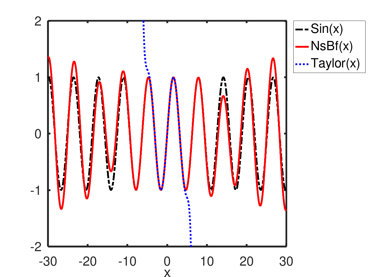
Figure 1: Approximation of $y=\sin\left(x\right)$ by the NsBf and by the Taylor series with the value of the function and values of the first ten derivatives matched.

Approximation of Padé

The Padé partial approximation by a rational function is a rather well-known example which does not fall into any category of Sec. 2. The approximation $\mathcal{A}_{N}^{f,P}$ is build as a ratio of two polynomials

$$\mathcal{A}_{m+n+1}^{f,P}(x)=\frac{P_{m}(x)}{P_{n}(x)},\>P_{m}(x)=\sum_{i=0}^{m}a_{1,i}^{[m+n+1]}x^{i},\>P_{n}(x)=1+\sum_{j=1}^{n}a_{2,j}^{\left[m+n+1\right]}x^{j},$$

where the absolute term of $P_{n}$ is (by definition) one. The approximation is, to the author’s knowledge, always used as partial, which may be understood as the consequence of its complicated character (non-persistent coefficients). The coefficients $a_{1,i}^{[m+n+1]}$, $a_{2,i}^{[m+n+1]}$ can be determined in a “brute-force” manner by differentiating $\mathcal{A}_{m+n+1}^{f,P}$ and solving the resulting equations, even though more efficient methods are on the market, see [10]. The latter reference corresponds to one of the large number of texts which cover Padé approximation and where further information (e.g. about the convergence issues) can be found.

The Padé approximants are known to have good convergence properties, in some situations the domain of the convergence extends beyond that of the Taylor series. Often, the Padé approximation converges more rapidly than the Taylor series which explains its popularity in numerical computations [11]. These appealing features are attributed to the fact that the form of rational functions enables the approximation to mimic the poles (and branch cuts [12]) of the approximated functions.

We discuss further this topic also in Sections 4.1.2 and 4.1.3 where we introduce presumably new ways of constructing a rational approximation.

Powers of sines

The derivative-matching approach can be applied also to trigonometric polynomials [13]. One has

$$\mathcal{A}_{n}^{f,S}(x)=a_{0}+\sum_{n=1}^{\infty}a_{n}\left[\sin\left(\frac{x}{2}\right)\right]^{n}$$ (8)

with

$$a_{0}=c_{0}^{f},\quad a_{n}=\frac{2^{n}}{n!}\sum_{k=1}^{n}c_{k}^{f}\left|t(n,k)\right|$$

where $t(n,k)$ are the central factorial numbers of the first kind defined by the equation

$$x\left(x+\frac{n}{2}-1\right)\left(x+\frac{n}{2}-2\right)\ldots\left(x-\frac{n}{2}+1\right)=\sum_{k=0}^{n}t\left(n,k\right)x^{k},\quad n\epsilon\mathbb{N}.$$

The expansion is certainly interesting, the use of trigonometric power formulas allows one to transform (8) into a formal Fourier series on $\left(-2\pi,2\pi\right)$, yet not constructed by scalar products but upon “Taylor’s” principles. The authors of [13] study in details the convergence properties of this series and also claim that such an expansion may be useful, e.g. in the theory of trigonometric asymptotic expansions. The approximation (8) is triangular and represents a special case of a larger group of approximations which we address in Sec. 4.1.2.

3.2 Matching re-weighted integrals

A large family of approximations is based on integrals where the integrand is the product of the approximated function and a function which belongs to some predefined (usually infinite) function set

$$\mathcal{C}_{n}=\int_{a}^{b}dx\,\left[v_{n}\left(x\right)\times\ldots\right]\quad c_{n}^{f}=\int_{a}^{b}v_{n}\left(x\right)f\left(x\right)\,dx,\quad v_{n}\epsilon V\equiv\left\{v_{i}\right\}_{i=0}^{\infty}.$$ (9)

Most of these approximations are usually formally interpreted in terms of a vector space of functions where the integral defines the scalar product and $V$ represents a complete orthonormal basis. There are exceptions, e.g. such an interpretation is not adopted for the moment problem, yet the (raw) moments are also computed as re-weighted function integrals.

The vector-space based approximations are numerous, extend to more dimensions (e.g. the spherical harmonics $Y_{l}^{m}\left(\theta,\varphi\right)$) with many different basis, thus the following examples should be understood as basic illustrative examples for this group of approximations. The orthonormality of the basis corresponds to the delta property of the approximation.

Fourier series and generalized Fourier series

Let us in parallel present the two most common “vector-space” approximations, the Fourier series ($\mathcal{A}^{f,F}$) and the Legendre-Fourier series ($\mathcal{A}^{f,L}$) defined on their usual intervals $\left(-\pi,\pi\right)$ and $\left(-1,1\right)$ respectively. One has

$$\mathcal{A}^{f,F}\left(x\right)=\sum_{n=0}^{\infty}a_{n}v_{n},\quad v_{n}=\Delta_{n}=\begin{cases}\frac{1}{\sqrt{2}}&\text{for }n=0\\ \sin\left(\frac{n+1}{2}x\right)&\text{for }n=1,3,5,\ldots\\ \cos\left(\frac{n}{2}x\right)&\text{for }n=2,4,6,\ldots\end{cases},$$

$$\mathcal{A}^{f,L}\left(x\right)=\sum_{n=0}^{\infty}a_{n}v_{n},\quad v_{n}=\Delta_{n}=\sqrt{\frac{2}{2n+1}}P_{n},$$

where $P_{n}$ are the Legendre polynomials. Both approximations are delta approximations based on linear functionals and delta functions. The relation to characteristic numbers stands

$$a_{n}=c_{n}^{f}.$$ (10)

This approach generalizes to other expansions, such as Fourier–Bessel series, series of spherical harmonics (Laplace series), Schlömilch’s series, etc. Since $\left\{v_{i}\right\}_{i=0}^{\infty}$ represents a complete basis of a normed vector space, the series convergence in the norm ($L^{p}$) implies an almost everywhere pointwise convergence.

The Fourier series and their generalizations are very useful in many different areas of mathematics and physics, among the most important are the frequency analysis or solution techniques for differential equations. The approximation by Fourier series is limited to periodic functions.

Moments

The raw moments are defined by

$$v_{n}=x^{n}.$$

We conjecture that the delta functions cannot be constructed and prove it for stronger assumptions hereunder. The construction of the approximation $\mathcal{A}^{f,M}$ from the characteristic numbers (i.e. the raw moments) is a well-known moment problem [15]. The approach we present is however more general (than the classical moment problem), since, in the latter, one usually assumes $f$ to be positive, which we do not do here. Depending on the interval, the moment problem is labeled as Hamburger ($a=-\infty,\>b=\infty$), Stieltjes ($a=0,\>b=\infty$) or Hausdorff (both $a$ and $b$ finite). For illustration purposes we choose the latter and (without loss of generality) assume $a=-1$, $b=1$ (and a general, possibly negative $f$). In this context we prove

Proposition 1.

The set $\left\{\Delta_{n}\right\}_{n=0}^{\infty}$ cannot be constructed from continuous functions expressible as Fourier-Legendre series.

Proof.

We proceed by contradiction and assume the existence of such $\Delta_{n}$ for all $n\epsilon\mathbb{N}_{0}$

$$\Delta_{n}(x) =\sum_{i=0}^{\infty}\alpha_{i}^{n}L_{i}(x),\quad\alpha_{i}^{n}=\int_{-1}^{1}\Delta_{n}(x)L_{i}(x)dx=2^{i}\sqrt{\frac{2}{2i+1}}\binom{i}{n}\binom{\frac{i+n-1}{2}}{i},$$

where $\left\{L_{i}\right\}$ is an orthonormal basis $L_{i}=\sqrt{\frac{2}{2i+1}}P_{i}$ ($P_{i}$ being the Legendre polynomials), the brackets denote the generalized form of the binomial coefficient and we use (after writing $L_{i}(x)$ as polynomial) the assumed delta property of $\Delta_{n}$. Let us investigate the value of $\Delta_{n}$ at $x_{0}=0$ for some even $n=2m$. One has

$$\Delta_{2m}(0) =\sum_{j=0}^{\infty}\alpha_{j}^{2m}L_{j}(0)=\sum_{j=0}^{\infty}\left(-1\right)^{j}\frac{2}{4j+1}\binom{2j}{2m}\binom{j+m-\frac{1}{2}}{2j}\binom{2j}{j}\equiv\sum_{j=0}^{\infty}q_{j}^{m}.$$

Re-writing an individual sum element in terms of factorials (using the factorial expressions for $\Gamma\left[\frac{1}{2}\pm n\right]$) one can study the large-$j$ behavior ($j\geq m$)

$$q_{j}^{m} =\frac{\left(-1\right)^{m}}{4^{2j}}\>\frac{2}{4j+1}\>\frac{\left(2j\right)!}{\left(2m\right)!\left(j!\right)^{2}}\>\frac{\left(2j+2m\right)!}{(j+m)!(j-m)!}.$$

The limit $j\rightarrow\infty$ is easily determined by taking the logarithm and using the Stirling’s approximation of the factorial

$$\lim_{j\rightarrow\infty}\ln\left[\left(-1\right)^{m}q_{j}^{m}\right]=\infty.$$

Thus $\Delta_{n}$ is (at zero and at least for some $n$) either not defined (i.e. continuous) or not expressible as Fourier-Legendre series. Both cases contradict the assumptions. ∎

Continuous partial delta functions $\Delta_{m}^{[N],M}$ can be found by assuming (for example) a polynomial form and by solving equations (5), or by combining the Legendre polynomials in an appropriate way so that the partial-delta behavior is obtained (as demonstrated in the next paragraph). Numerical results suggest that the expressions for $\Delta_{n}^{\left[N\rightarrow\infty\right]}$ diverge almost everywhere on $\left(-1,1\right)$.

The moment-matching problem can be solved using a triangular approximation, one example of such is represented by the Fourier-Legendre series [16, 17, 18]. The Legendre polynomials $P_{m}=\nabla_{m}$ obey the triangular property (3)

$$\int_{-1}^{1}P_{m}x^{n}dx=0\text{ for all }n<m$$ (11)

and any partial approximation of $f$ of the order $N$ matches its first $N+1$ moments. Indeed, if $f$ is expanded on $(-1,1)$ into the series

$$f\left(x\right)=\sum_{n=0}^{N}\beta_{n}P_{n}\left(x\right),$$ (12)

then $m$th moment of the latter ($0\leq m\leq N$) is given by

$$\int_{-1}^{1}dx\>x^{m}\sum_{n=0}^{N}\beta_{n}P_{n}\left(x\right)=$$

$$\quad=\int_{-1}^{1}dx\>x^{m}\sum_{n=0}^{N}\left(\frac{2n+1}{2}\int_{-1}^{1}dy\>f\left(y\right)P_{n}\left(y\right)\right)P_{n}\left(x\right),$$

$$\quad=\int_{-1}^{1}dx\>x^{m}\int_{-1}^{1}dy\>f\left(y\right)\left[\sum_{n=0}^{\infty}\frac{2n+1}{2}P_{n}\left(y\right)P_{n}\left(x\right)-\sum_{n=N+1}^{\infty}\frac{2n+1}{2}P_{n}\left(y\right)P_{n}\left(x\right)\right],$$

$$\quad=c_{m}^{f},$$

where we used the completeness property

$$\sum_{n=0}^{\infty}\frac{2n+1}{2}P_{n}\left(y\right)P_{n}\left(x\right)=\delta\left(x-y\right)$$

for the left term in the square brackets and the property (11) for the right one (we assume $f$ such that the order of integrals and summation can be changed and the integration over $dx$ performed first). In the expansion (12) the coefficients can be directly related to the (known) polynomial coefficients $\gamma_{j}^{n}$ of $P_{n}$ and moments $c_{j}^{f}$ of $f$

$$\beta_{n} =\frac{2n+1}{2}\int_{-1}^{1}f\left(x\right)P_{n}\left(x\right)dx=\frac{2n+1}{2}\int_{-1}^{1}f\left(x\right)\sum_{j=0}^{n}\gamma_{j}^{n}x^{j}dx$$ (13)

$$=\frac{2n+1}{2}\sum_{j=0}^{n}\gamma_{j}^{n}\int_{-1}^{1}f\left(x\right)x^{j}dx=\frac{2n+1}{2}\sum_{j=0}^{n}\gamma_{j}^{n}c_{j}^{f}$$

with

$$\gamma_{j}^{n}=2^{n}\binom{n}{j}\binom{\frac{n+j-1}{2}}{n}.$$ (14)

Furthermore, by choosing $\left(\overrightarrow{c_{m}^{f}}\right)_{j\leq N}=\delta_{m,j}$, one can construct partial delta functions

$$\Delta_{m}^{[N],M}=\sum_{n=0}^{N}\beta_{n}\left(\overrightarrow{c_{m}^{f}}\right)P_{n}\left(x\right).$$ (15)

Numerical computations suggest (Fig. 2) that the Legendre-Fourier series of many common functions converge to the function also outside the $(-1,1)$ interval, which would be a distinctive feature from the standard Fourier series. This observations needs to be supported by rigorous arguments.

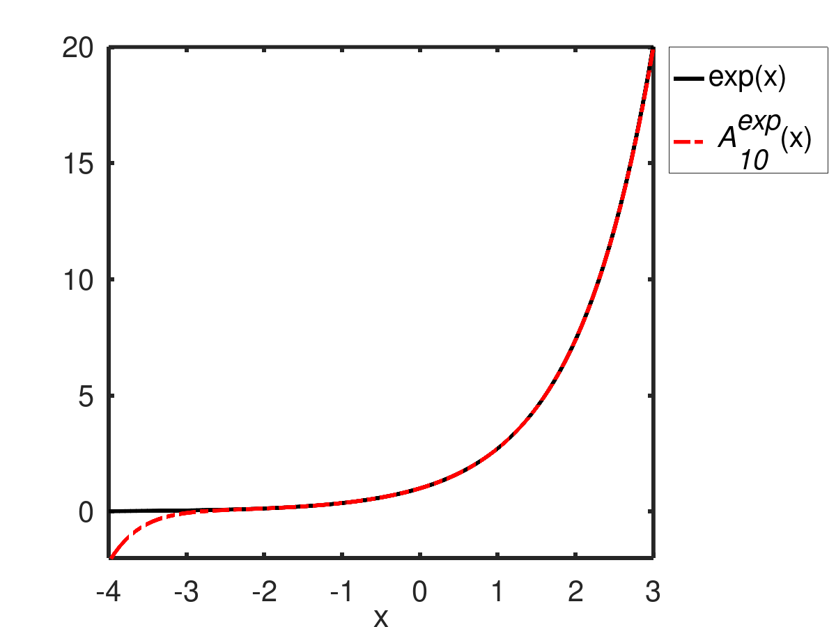
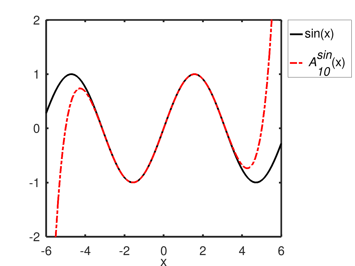
Figure 2: Examples of Legendre-Fourier expansions interpreted as triangular moment-matching approximations shown on an interval larger than $\left(-1,1\right)$.

The notion of the moment can be generalized, the generalization is often constructed as an integral where the power of $x$ is replaced by an orthogonal polynomial (for an overview see [19]). The importance of the moment expansion is derived from the importance of the moments themselves: they are widely used in probability theory, statistics, physics and many other fields too.

Higher integrals

With the Taylor series being one of the most popular expansions, one can ask whether a similar approximation based on higher-order integrals (and not higher-order derivatives) could be constructed. However, because of the integration constant freedom, the value of an anti-derivative is not fixed. One can overcome this by setting its value in some arbitrary way. For our purposes we define

$$\mathcal{C}_{n}\left(f\right)\equiv c_{n}^{f}=f^{(-n)}(1),\quad\frac{d}{dx}f^{(-n)}(x) =f^{(-n+1)}(x),\quad f^{(-n)}(-1)=0,$$ (16)

$$\text{ for all }n>0.$$

Even though new at the first sight (and maybe appropriate rather for Sec. 4), this approximation can be related to the moment-matching problem by the means of the Cauchy repeated-integral formula. One has

$$f^{(-n)}(1)\equiv c_{n}^{f}=\frac{1}{\left(n-1\right)!}\int_{-1}^{1}\left(1-t\right)^{n-1}f\left(t\right)dt.$$

By subsequent substitutions $z=1-t$, $g\left(z\right)=f\left(1-z\right)$, $w=z/2$ and $h(w)=g(2w)$ we arrive to

$$c_{n}^{f}=\frac{1}{\left(n-1\right)!}\int_{0}^{2}z^{n-1}g\left(z\right)dz=\frac{2^{n}}{\left(n-1\right)!}\int_{0}^{1}w^{n-1}h\left(w\right)dw\equiv\frac{2^{n}}{\left(n-1\right)!}m_{n-1}^{h}.$$

One can define $m_{n}^{h}=n!c_{n+1}^{f}/2^{n+1}$ ($n=0,1,\ldots$) and interpret the latter as moments computed on the interval $\left(0,1\right)$. The construction of all objects (approximations, delta functions) on this interval is fully analogous to $\left(-1,1\right)$, only the set of orthogonal polynomials is now represented by the shifted Legendre polynomials $P_{n}^{\left(0,1\right)}$ and expressions (13) and (14) are modified

$$\widetilde{\beta}_{n}=\left(2n+1\right)\int_{0}^{1}f\left(x\right)P_{n}^{\left(0,1\right)}dx,\quad\widetilde{\gamma}_{j}^{n}=\left(-1\right)^{n+j}\binom{n}{j}\binom{n+j}{j}.$$

By building a moment-matching approximation $\mathcal{A}^{h,M}\left(x\right)$ of $h$, a higher-integral approximation $\mathcal{A}^{f,I}$ of $f$ can be constructed

$$\mathcal{A}^{f,I}\left(x\right)=\mathcal{A}^{h,M}\left(\frac{1-x}{2}\right).$$

One may notice, that, unlike for the Taylor polynomials, the rules (16) do not fix the function value at $x=1$ (are not applied at the zeroth order $n=0$). Indeed, the moments $\left\{m_{n}^{h}\right\}_{n=0}^{\infty}$ fully determine the function $h$ (not only its shape but also its normalization) and thus $f$.

3.3 Matching integrals of higher-order derivatives

An approximation can be constructed upon functionals

$$\mathcal{C}_{n}=\int_{a}^{b}dx\,\frac{d^{n}}{dx^{n}},\;c_{n}^{f}=\int_{a}^{b}f^{\left(n\right)}\left(x\right)\,dx\equiv f^{\left(n-1\right)}\left(b\right)-f^{\left(n-1\right)}\left(a\right).$$

Bernoulli polynomial series

Choosing this time $a=0$ and $b=1$, one can find an approximation $\mathcal{A}^{f,B}$ constructed as a series with multiplicative coefficients based on delta functions

$$\mathcal{A}^{f,B}(x)=\sum_{n=0}^{\infty}a_{n}\Delta_{n}(x),\quad\Delta_{n}(x)=\frac{1}{n!}B_{n}\left(x\right),$$

where $B_{n}$ are the Bernoulli polynomials. The matching is done by setting

$$a_{n}=c_{n}^{f}.$$

A peculiar situation happens for $n=0$, where one needs to compute an integral. However the $c_{0}$ coefficient corresponds only to a global shift (up/down) of $f$, because $B_{0}\left(x\right)$ is just a constant. Thus the integration can be avoided: one can build the expansion $\mathcal{A}_{n>0}^{f,B}(x)$ for all $n>0$ and then adjust the normalization by matching the value at some point $0\leq x_{0}\leq 1$

$$\mathcal{A}^{f,B}(x)=\mathcal{A}_{n>0}^{f,B}(x)+f(x_{0})-\mathcal{A}_{n>0}^{f,B}(x_{0}).$$

Ignoring the latter complication, the expansion has a lot of beauty since it is almost as easy to build as the Taylor series, one only needs to know the derivatives at two points instead of one. Despite the simplicity, it seems not to be known very well, although appearing in the literature at several places [20, 21, 22]. One can consult the latter reference to address the convergence questions. Some problems regarding the convergence can be easily seen when realizing how the delta functions are constructed. One can formally introduce a function $\Delta_{-1}$ satisfying

$$\mathcal{C}_{n}\left(\Delta_{-1}\right)=0\text{ for all }n\geq 0.$$ (17)

By integration one defines functions $\Delta_{n\geq 0}$, $\Delta^{\prime}_{n+1}=\Delta{}_{n}$ and by a careful choice of integration constants one can fulfill the delta property $\mathcal{C}_{n}\left(\Delta_{m}\right)=\delta_{n,m}$. A natural choice $\Delta_{-1}(x)\equiv 0$ leads to the Bernoulli polynomials. However there are other functions, such as for example $\cos\left(2\pi x-\pi\right)$, which also fulfill (17) and which would lead, performing the integration, to different delta functions. Thus one cannot expect the Bernoulli-polynomials based expansion to converge for $\cos\left(2\pi x-\pi\right)$ on $\left(0,1\right)$.

The approximation can be scaled to an arbitrary finite interval $\left(a,b\right)$ by scaling the argument

$$\mathcal{A}_{\left(a,b\right)}^{f,B}(x)=\sum_{n=0}^{\infty}a_{n}\Delta_{n}^{\left(a,b\right)}(x),\quad\Delta_{n}^{\left(a,b\right)}(x)=\left(b-a\right)^{n-1}\Delta_{n}(\frac{x-a}{b-a}).$$

A natural question rises about the behavior of $\mathcal{A}_{\left(a,b\right)}^{f,B}$ for $b\rightarrow a$.

Proposition 2.

For an analytic function $f$, the partial approximation $\mathcal{A}_{\left(a,b\right),N}^{f,B}$ becomes in the limit $b\rightarrow a$ its Taylor polynomial.

Proof.

Using the notation $b=a+\varepsilon$, straightforward computations yield

$$\mathcal{A}_{\left(a,a+\varepsilon\right),N}^{f,B}=\sum_{n=0}^{N}\left[f^{\left(n-1\right)}\left(a+\varepsilon\right)-f^{\left(n-1\right)}\left(a\right)\right]\varepsilon^{n-1}\frac{1}{n!}B_{n}\left(\frac{x-a}{\varepsilon}\right).$$

Writing $f^{\left(n-1\right)}\left(a+\varepsilon\right)=f^{\left(n-1\right)}\left(a\right)+\varepsilon f^{\left(n\right)}\left(a\right)+\mathcal{O}\left(\varepsilon^{2}\right)$ and using the notation $f^{\left(n\right)}\equiv f^{\left(n\right)}\left(a\right)$ one has

$$\mathcal{A}_{\left(a,a+\varepsilon\right),N}^{f,B}=\sum_{n=0}^{N}\left[\varepsilon f^{\left(n\right)}+\mathcal{O}\left(\varepsilon^{2}\right)\right]\varepsilon^{n-1}\frac{1}{n!}\sum_{k=0}^{n}\frac{n!}{(n-k)!k!}B_{n-k}\varepsilon^{-k}\left(x-a\right)^{k},$$

where explicit formulas for the Bernoulli polynomials were used with $B_{n-k}$ denoting the Bernoulli numbers. Re-arranging the sums one arrives to

$$\mathcal{A}_{\left(a,a+\varepsilon\right),N}^{f,B}=\sum_{k=0}^{N}\frac{1}{k!}\left\{\sum_{n=k}^{N}\varepsilon^{n-k}\frac{f^{\left(n\right)}+\mathcal{O}\left(\varepsilon\right)}{(n-k)!}B_{n-k}\right\}\left(x-a\right)^{k},$$ (18)

One can study an individual term in front of the powers of $\left(x-a\right)$ in the limit $\varepsilon\rightarrow 0$. In this limit the dominant $\varepsilon$ term is the one where $n=k$. Thus we have

$$\lim_{\varepsilon\rightarrow 0}\sum_{n=k}^{N}\varepsilon^{n-k}\frac{f^{\left(n\right)}+\mathcal{O}\left(\varepsilon\right)}{(n-k)!}B_{n-k}\overset{n=k}{=}f^{\left(k\right)}$$

leading to

$$\lim_{\varepsilon\rightarrow 0}\mathcal{A}_{\left(a,a+\varepsilon\right),N}^{f,B}=\sum_{k=0}^{N}\frac{1}{k!}f^{\left(k\right)}\left(x-a\right)^{k}$$

which corresponds to the Taylor polynomial. ∎

Assuming the re-arrangement of the sums (18) is justified for $N=\infty$, the whole proof is valid for a full approximation and the Taylor series. Also, the analyticity condition can be presumably relaxed if the error in the small parameter expansion of $f^{\left(n-1\right)}\left(\varepsilon\right)$ is treated carefully. Numerical observations indicate a rich set of interesting properties which await to be addressed rigorously:

• Functions such as $\cos\left(x\right)$ do not have (as expected) a convergent approximation $\mathcal{A}_{\left(a,b\right)}^{f,B}$ for $b-a=2\pi$. However, if the length of the interval differs only slightly from (a multiple of) $2\pi$, the approximation seems to converge.

• Numerical computations suggest that for many common functions the approximation $\mathcal{A}_{\left(a,b\right)}^{f,B}$ fails to converge once the interval length goes over some limit. For $\exp\left(x\right)$ approximated on a symmetric interval $\left(-a,a\right)$ the convergence seems to be lost for $a\apprge\pi$.

• The quality of partial approximations $\mathcal{A}_{N}^{f,B}$may increase with increasing $N$ up to some $N_{0}$, and decrease (become divergent) afterwards. Such behavior is observed for $f(x)=\sqrt{4-x^{2}}$ approximated on $\left(-1,1\right)$ where the best-quality partial approximation $\mathcal{A}_{\left(-1,1\right),N}^{f,B}$ is realized for $N=4$ and $N=5$.

3.4 Value matching

Approximations (often partial) meant to match function values

$$\mathcal{C}_{n}\left(f\right)=f\left(x_{n}\right),\;c_{n}^{f}=f\left(x_{n}\right),\;\left\{x_{n}\right\}_{n=0}^{N,\infty},\;x_{n}\epsilon\left(a,b\right),$$

where $\left\{x_{n}\right\}$ is a predefined set of numbers, are usually referred to as interpolations and represent a very large topic covered by many resources. Hence, we present only the most popular ones, among them the Lagrange form of the interpolation polynomial. It is a delta approximation

$$\mathcal{A}_{N}^{f,V}(x)=\sum_{n=0}^{N}a_{n}\Delta_{n}(x),\quad\Delta_{n}(x)=\prod_{i=0,i\neq n}^{N}\frac{(x-x_{i})}{(x_{n}-x_{i})},\;a_{n}=c_{n}^{f},$$

where the delta property is reached by the creation of zeros in the numerator for all $\left\{x_{i}\right\}$ except $x_{n}$. The denominator then guarantees a correct normalization $\Delta_{n}(x_{n})=1$. The Newton form of the interpolation polynomial is a modification of the previous and provides a triangular approximation

$$\mathcal{A}_{N}^{f,V^{\prime}}(x)=\sum_{n=0}^{N}a_{n}\nabla_{n}(x),\quad\nabla_{n}(x)=\prod_{i=0}^{n-1}(x-x_{i}),\;a_{n}=a_{n}\left(c_{0}^{f},\ldots,c_{n}^{f}\right)$$

for which the individual terms of the sum are defined also in the limit $N\rightarrow\infty$, the coefficients $a_{n}$ are divided differences. The idea of creating zeros can be generalized and an approximation built using an arbitrary function $\rho$ such that $\rho\left(0\right)=0$

$$\mathcal{A}_{N}^{f,V^{\prime\prime}}\left(x\right)=\sum_{n=0}^{N}c_{n}^{f}\prod_{k=0,k\neq n}^{N}\frac{\rho\left(x-x_{k}\right)}{\rho\left(x_{n}-x_{k}\right)}.$$

For $\rho\left(x\right)=\sin\left(x\right)$ this leads to a trigonometric interpolation (of a non-minimal degree) and Fourier series.

Several other approximations can be found on the market, usually less popular (e.g. the Whittaker–Shannon interpolation formula, which we address in Sec. 4.3 or [23]). Nevertheless a number of theoretical results have been derived in this domain, most of them related to the existence of an entire function (in the complex plane) with the interpolation property. One can mention e.g. the Nevanlinna–Pick problem [24] or the Weierstrass factorization theorem (which turns $f$ into an infinite product).

This kind of approximations can be useful for functions which are easy to evaluate on some countable set of their arguments, thus providing a way to approximate them elsewhere. The structure of this set is usually specified by the method itself (e.g. equidistant points for the Whittaker–Shannon formula) and cannot be later changed to suit the function.

4 New examples

4.1 Matching derivatives

In this sub-section we present new approximations based on the derivative matching

$$c_{n}^{f}=\frac{d^{n}f\left(x\right)}{dx^{n}}|_{x=x_{0}=0}.$$

We propose three expansions exploiting a similar idea which is to build a series with multiplicative coefficients where, by construction, the coefficients enter into the game progressively when higher order derivatives are performed (i.e. the approximations are triangular). The fourth example is somewhat different, it deals with a partial delta approximation.

4.1.1 Expansion into $g\left(x\right)\sum a_{n}x^{n},\;g\left(0\right)\neq 0$

An approximation of the form

$$\mathcal{A}^{f}\left(x\right)=g\left(x\right)\sum_{n=0}^{\infty}a_{n}x^{n},\;g\left(0\right)\neq 0$$ (19)

is triangular because, following the product and chain differentiation rules, the term $g\left(x\right)x^{n}$ becomes non-zero only after $n$ differentiations. To make a connection between power-expansion coefficients of $f$, $f_{n}=c_{n}^{f}/n!$ and those of $g$, $g_{n}=g^{\left(n\right)}\left(0\right)/n!$ let us assume that both functions are analytic. Then, the Cauchy product of $\sum a_{k}x^{k}$ and $g\left(x\right)=\sum g_{k}x^{k}$ on the right-hand side of (19) yields

$$\sum_{k=0}^{\infty}f_{k}x^{k}\overset{!}{=}\sum_{k=0}^{\infty}\left[\sum_{n=0}^{k}a_{n}g_{k-n}\right]x^{k},$$

where the expression in the square brackets corresponds to a lower triangular Toeplitz matrix

$$\left(\begin{array}[]{c}f_{0}\\ f_{1}\\ f_{2}\\ \vdots\end{array}\right)=\left(\begin{array}[]{cccc}g_{0}&0&0&\cdots\\ g_{1}&g_{0}&0&\cdots\\ g_{2}&g_{1}&g_{0}&\cdots\\ \vdots&\vdots&\vdots&\ddots\end{array}\right)\left(\begin{array}[]{c}a_{0}\\ a_{1}\\ a_{2}\\ \vdots\end{array}\right).$$

To invert the matrix a recursive formula based on generalized Fibonacci polynomials is available [25]. The $a_{n}$ coefficients in (19) are expressed in terms of $g_{n}$ and $f_{n}$ as follows

$$a_{n}=\frac{1}{g_{0}}\sum_{i=0}^{n}\Lambda_{n-i}f_{i},\text{ where }\varLambda_{k}=\begin{cases}1&\text{ if }k=0\\ -\left(\sum_{j=1}^{k}g_{j}\varLambda_{k-j}\right)/g_{0}&\text{else}\end{cases}.$$

The expansion can be shifted to an arbitrary point $x_{0}\epsilon\mathbb{R}$ by shifting its argument. One also notes that the expansion is equivalent to building the Taylor series for $h(x)\equiv f(x)/g\left(x\right)$, its novelty lies in finding the relation between the coefficients $\left\{a_{i}\right\}$ and the derivatives of $f$ (an not those of $h$). In order to provide an example without recurrent relations we chose $g\left(x\right)=\exp\left(wx^{q}\right)$ and prove

Proposition 3.

A smooth function $f$can be approximated at $x_{0}=0$ by

$$\mathcal{A}^{f,D_{1}}\left(x\right)=\exp\left(wx^{q}\right)\sum_{n=0}^{\infty}a_{n}x^{n},\quad q\epsilon\mathbb{N^{+}},w\epsilon\mathbb{R},$$ (20)

with

$$a_{n}=\sum_{i=0}^{n}m_{n,i}c_{i}^{f},\quad m_{n,i}=\delta_{v_{n-i},0}\frac{\left(-1\right)^{u_{n-i}}w^{\left\llbracket u_{n-i}\right\rrbracket}}{\left(v_{n}+qu_{i}\right)!u_{n-i}!},$$ (21)

$$u_{n}=\left\lfloor\frac{n}{q}\right\rfloor,\quad v_{n}=n\%q\text{ and }x^{\left\llbracket y\right\rrbracket}=\begin{cases}1&\text{\text{for }}x=y=0\\ x^{y}&\text{else (when defined)}\end{cases},$$

where $\left\lfloor\>\right\rfloor$ is the floor function, $\%$ represents the modulo operation and the generalized exponentiation allows (otherwise undefined) expansion for cases $w=0$.

Proof.

Using the general Leibniz rule we differentiate (20) $m$ times

$$\frac{d^{m}}{dx^{m}}\left[\exp\left(wx^{q}\right)\sum_{n=0}^{\infty}a_{n}x^{n}\right]=\sum_{k=0}^{m}\binom{m}{k}\left[\sum_{n=0}^{\infty}a_{n}x^{n}\right]^{(m-k)}\left[\exp\left(wx^{q}\right)\right]^{(k)}.$$

The first factor becomes

$$\left[\sum_{n=0}^{\infty}a_{n}x^{n}\right]_{x=0}^{(m-k)}=\left[\sum_{n=0}^{\infty}\frac{(n+m-k)!}{n!}a_{n+m-k}x^{n}\right]_{x=0}=(m-k)!a_{m-k},$$

where we are interested in the absolute term which determines the derivative at zero. The second factor can be deduced from the repeated differentiation of the corresponding power expansion. One has

$$\left[\frac{d^{k}}{dx^{k}}\exp\left(wx^{q}\right)\right]_{x=0}=\left[\frac{d^{k}}{dx^{k}}\sum_{n=0}^{\infty}\frac{1}{n!}\left(wx^{q}\right)^{n}\right]_{x=0}=\delta_{v_{k},0}w^{u_{k}}\frac{(u_{k}q)!}{u_{k}!}.$$

Combining the two results one arrives at

$$\frac{d^{m}}{dx^{m}}\left[\exp\left(wx^{q}\right)\sum_{n=0}^{\infty}a_{n}x^{n}\right]_{x=0} =\sum_{j=0}^{m}\delta_{v_{m-j},0}\frac{m!(u_{m-j}q)!}{(m-j)!u_{m-j}!}w^{u_{m-j}}a_{j},$$ (22)

$$\equiv\sum_{j=0}^{m}D_{m,j}a_{j},$$

which gives derivatives as a function of the coefficients $a_{j}$. Using the matrix language (and defining $D_{m,j}=0$ for $j>m$), the dependence of coefficients on derivatives is provided by $D^{-1}$. One has

$$\left(D^{-1}\right)_{n,i\leq n}=\delta_{v_{n-i},0}\frac{\left(-1\right)^{u_{n-i}}w^{\left\llbracket u_{n-i}\right\rrbracket}}{\left(v_{n}+qu_{i}\right)!u_{n-i}!}$$ (23)

with $\left(D^{-1}\right)_{n,i>n}=0$. The (infinite) matrices $D$ and $D^{-1}$ are lower triangular, thus $\left(DD^{-1}\right)_{n,i>n}=0$. For $n=i$ the computation is straightforward ($u_{0}=0$, $v_{0}=0$)

$$\left(DD^{-1}\right)_{i,i} =\sum_{j=0}^{\infty}D_{i,j}\left(D^{-1}\right)_{j,i}=D_{i,i}\left(D^{-1}\right)_{i,i}=i!\times\frac{1}{\left(v_{i}+qu_{i}\right)!}=1.$$

A non-trivial computation arises for

$$\left(DD^{-1}\right)_{m,i<m} =\sum_{j=0}^{\infty}D_{m,j}\left(D^{-1}\right)_{j,i}=\sum_{j=i}^{m}D_{m,j}\left(D^{-1}\right)_{j,i}$$ (24)

The delta functions in (22) (23) imply $D$ and $D^{-1}$are block matrices with $q\times q$ sub-matrices which are diagonal. The $\left\{c_{k}^{f}\right\}$ and $\left\{a_{k}\right\}$ sets so split into $q$ subsets which transform independently and are characterized by the value of $w=0,\ldots,q-1$. One can write

$$\left(D_{w}^{\left(-1\right)}\right)_{p,k}\equiv\left(D^{\left(-1\right)}\right)_{w+pq,w+kq}$$

and analyze for $k<p$

$$\left(D_{w}D_{w}^{-1}\right)_{p,k} =\sum_{t=k}^{p}\left(D_{w}\right)_{p,t}\left(D_{w}^{-1}\right)_{t,k}$$

$$=\sum_{t=k}^{p}\frac{\left(w+pq\right)!(u_{w+pq-w-tq}q)!}{(w+pq-w-tq)!u_{w+pq-w-tq}!}w^{u_{w+pq-w-tq}}$$

$$\qquad\qquad\times\frac{\left(-1\right)^{u_{w+tq-w-kq}}w^{\left\llbracket u_{w+tq-w-kq}\right\rrbracket}}{\left(v_{w+tq}+qu_{w+kq}\right)!u_{w+tq-w-kq}!}$$

One has

$$u_{pq-tq} =p-t,\quad u_{tq-kq}=t-k,\quad v_{w+tq}=v_{w},\quad u_{w+kq}=u_{w}+k$$

which leads to

$$\left(D_{w}D_{w}^{-1}\right)_{p,k} =\sum_{t=k}^{p}\frac{\left(w+pq\right)!}{\left(p-t\right)!}w^{p-t}\times\frac{\left(-1\right)^{t-k}w^{\left\llbracket t-k\right\rrbracket}}{\left(w+qk\right)!\left(t-k\right)!}$$

$$=w^{p-k}\frac{\left(w+pq\right)!}{\left(w+qk\right)!}\sum_{t=k}^{p}\frac{\left(-1\right)^{t-k}}{\left(p-t\right)!\left(t-k\right)!}.$$

Using a substitution $s=t-k$ with the subsequent definition $r=p-k$ the latter sum becomes

$$\sum_{t=k}^{p}\frac{\left(-1\right)^{t-k}}{\left(p-t\right)!\left(t-k\right)!}=\sum_{s=0}^{r}\frac{\left(-1\right)^{s}}{\left(r-s\right)!s!}=\frac{1}{r!}\sum_{s=0}^{r}\left(-1\right)^{s}\binom{r}{s}=0.$$

The proof uses the standard exponentiation, the validity of the generalized exponentiation can be for $w=0$ easily checked. ∎

The special case $w=0$ corresponds to the Taylor series. The convergence properties can be derived from the criteria used for the Taylor series applied to the $\left\{a_{i}\right\}$ coefficients. Indeed, the exponential is an entire function in the whole complex plane and thus its power series converges absolutely at each complex point. Therefore, for a given $x$, the expression (20) can be interpreted as a multiplication of two sequences, one of which is absolutely convergent. Then, by the Mertens’ convergence theorem, the convergence of $\sum_{n=0}^{\infty}a_{n}x^{n}$ implies the convergence of the whole expression which converges to the product of the two series.

The proposed expansion may be interesting for several reasons. If one chooses, for example, an even and negative $w$, then each partial approximation approaches zero as $\left|x\right|\rightarrow\infty$ and has a finite integral over $\mathbb{R}$ (unlike e.g. the Taylor polynomials). Also, the structure as in (20) is very often to be seen in physics and mathematics, e.g. the radial parts of wave functions for commonly studied spherical potentials take in many cases this form. Also, if an extension to complex $q$ is possible (not studied here), the form of the approximation fits the definition of spherical harmonics. Example approximations using (20) are shown in Fig 3.

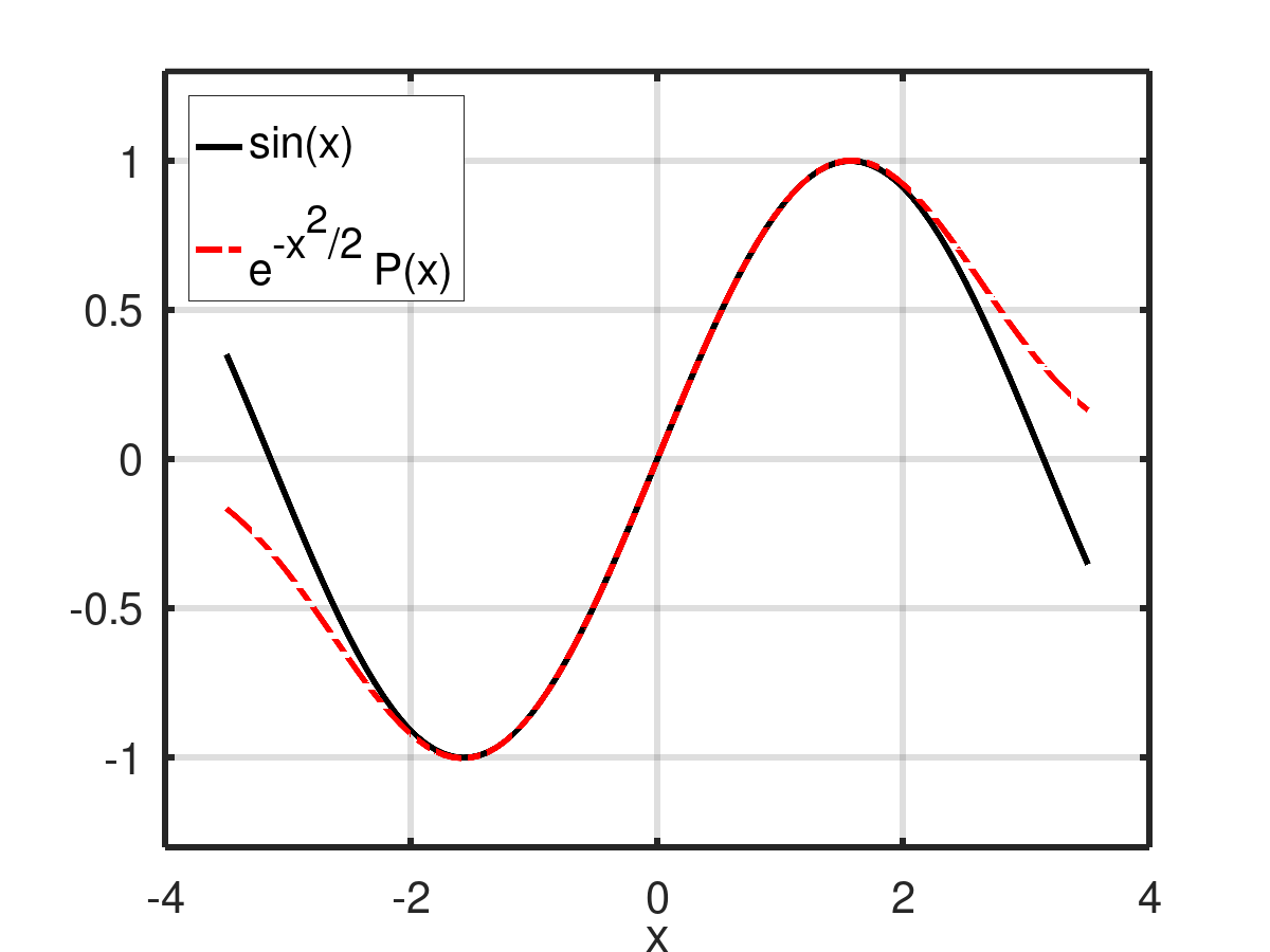
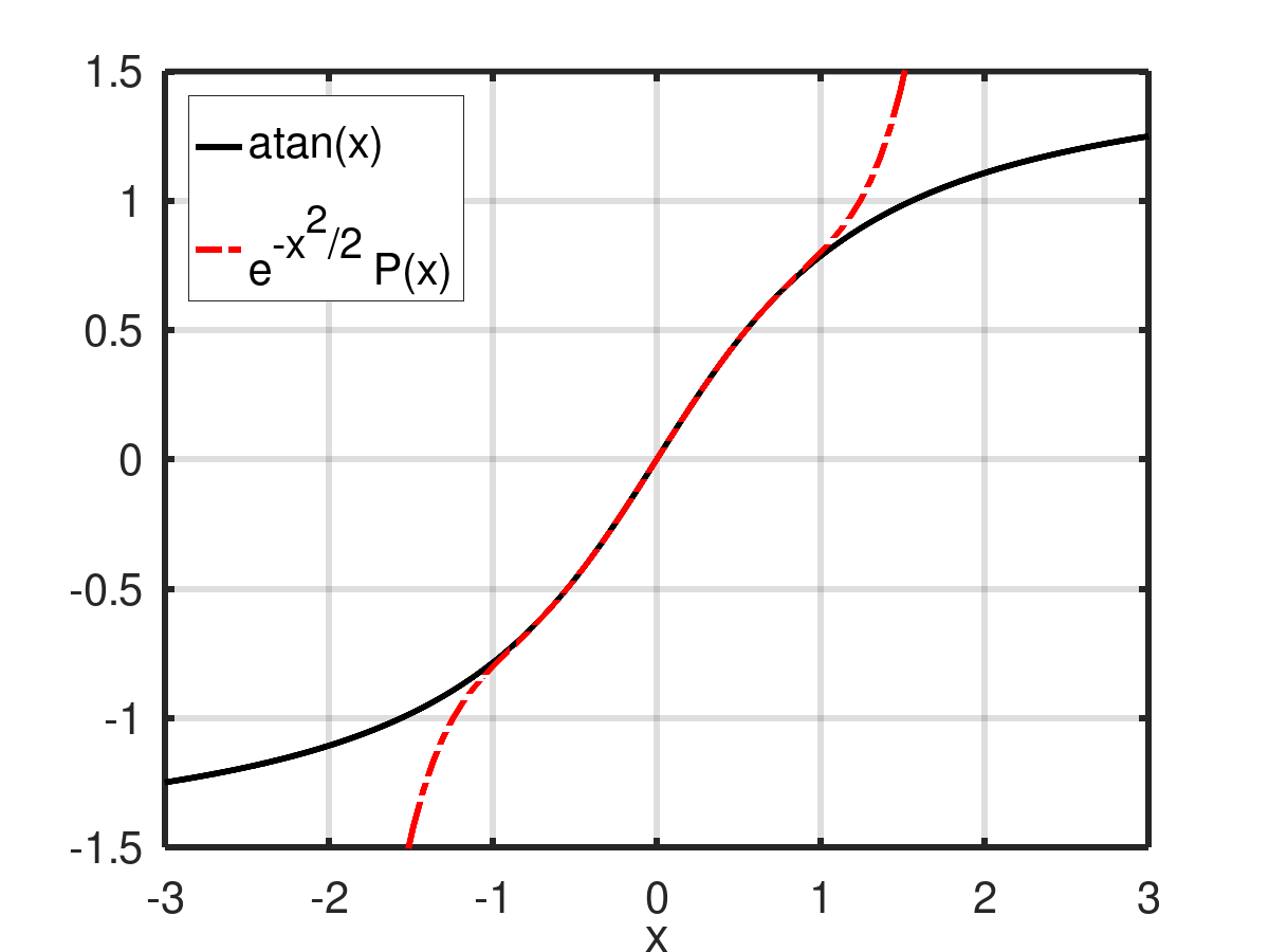
Figure 3: Approximating $\sin\left(x\right)$ and $\arctan\left(x\right)$ by expression (20) with 11 terms, $q=2$ and $w=-1/2$.

4.1.2 Expansion into $\sum a_{n}\left[g\left(x\right)\right]^{n},\;g\left(0\right)=0,\;g^{\prime}\left(0\right)\neq 0$

The next derivative-matching expansion we propose

$$\mathcal{A}^{f,D_{2}}\left(x\right)=\sum_{n=0}^{\infty}a_{n}\left[g\left(x\right)\right]^{n}\text{ with }\;g\left(0\right)=0\text{ and }g^{\prime}\left(0\right)\neq 0$$ (25)

uses a function $g$ which is for small $x\ll 1$ similar to $\alpha x$, $\alpha\neq 0$ (and thus invertible on some neighborhood of zero). It is a triangular approximation because, following the product and chain differentiation rules, the term $\left[g\left(x\right)\right]^{n}$ becomes non-zero only after $n$ differentiations. We encountered an example of this type in Sec. 3.1 which represents a special case with $g\left(x\right)=2\sin\left(x/2\right)$. Assuming the analyticity of $\mathcal{A}^{f,D_{2}}$ and its convergence to $f$, $\mathcal{A}^{f,D_{2}}=f$, one can introduce the substitution

$$x=g^{-1}\left(y\right)\text{ leading to }f\left(g^{-1}\left(y\right)\right)=\sum_{n=0}^{\infty}a_{n}y^{n}.$$

Thus $\left\{a_{n}\right\}$ can be obtained as the Taylor series coefficients of $f\left(g^{-1}\left(x\right)\right)$

$$a_{n}=\frac{1}{n!}\frac{d^{n}}{dx^{n}}f\left(g^{-1}\left(x\right)\right)|_{x=0}.$$ (26)

The complicated structure of higher-order derivatives of (26) makes an approach based on a general function $g$ impractical and one rather searches for feasible special cases.

Proposition 4.

One presumably new special case is represented by

$$\mathcal{A}^{f,D_{3}}\left(x\right)=\sum_{n=0}^{\infty}a_{n}\left[\ln\left(x+1\right)\right]^{n}$$ (27)

with

$$a_{n}=\frac{1}{n!}\sum_{k=0}^{n}c_{k}^{f}b_{n,k},\quad b_{n,k}=\frac{1}{k!}\sum_{i=0}^{k}\left(-1\right)^{i}\binom{k}{i}(k-i)^{\left\llbracket n\right\rrbracket},$$ (28)

where $b_{n,k}$ are the Stirling numbers of the second kind and $a^{\left\llbracket b\right\rrbracket}$ denotes the generalized exponentiation as introduced earlier.

Proof.

The Faà di Bruno’s formula can be written in terms of the power series of the composed function

$$f\left(g^{-1}\left(x\right)\right) =c_{0}^{f}+\sum_{n=1}^{\infty}\left[\frac{1}{n!}\sum_{k=1}^{n}c_{k}^{f}B_{n,k}\left(g_{1}^{-1},\ldots,g_{n-k+1}^{-1}\right)\right]x^{n},$$

$$g_{i}^{-1} \equiv\frac{d^{i}}{dx^{i}}g^{-1}\left(x\right)|_{x=0},$$

where $B_{n,k}$ are the Bell polynomials. We have $g^{-1}\left(x\right)=\exp\left(x\right)-1$ thus

$$g_{i>0}^{-1}=1$$

which leads to (26)

$$a_{n}=\frac{1}{n!}\frac{d^{n}}{dx^{n}}f\left(g^{-1}\left(x\right)\right)|_{x=0}=\frac{1}{n!}\sum_{k=1}^{n}c_{k}^{f}B_{n,k}(1,1,\ldots,1)=\frac{1}{n!}\sum_{k=1}^{n}c_{k}^{f}b_{n,k}.$$

The generalized exponentiation is used to define the $k=0$ case $b_{n,0}=\delta_{n,0}$ thus obtaining for all $n\geq 0$

$$a_{n}=\frac{1}{n!}\sum_{k=0}^{n}c_{k}^{f}b_{n,k}.$$

∎

The existence of various formulas involving the Bell polynomials, e.g.

$$B_{n,k}(0!,1!,\ldots,\left(n-k\right)!) =\left[\begin{array}[]{c}n\\ k\end{array}\right],$$ (31)

$$B_{n,k}(1!,2!,\ldots,\left(n-k+1\right)!) =\binom{n-1}{k-1}\frac{n!}{k!},$$ (32)

$$B_{n,k}(1,2,\ldots,n-k+1) =\binom{n}{k}k^{n-k},$$

implies the feasibility of the expansion (25) for those function $g^{-1}$ whose higher derivatives appear as arguments in these special cases. Choosing for example $g\left(x\right)=1-\exp\left(-x\right)$ one has $g^{-1}\left(x\right)=-\ln\left(1-x\right)$ of which the derivatives (at zero) appear in the first of the three formulas. In such a scenario $b_{n,k}=\left[\begin{smallmatrix}n\\ k\end{smallmatrix}\right]$. In the second of the three formulas the factorials are just shifted, thus leading to $g\left(x\right)=x/\left(x+1\right)$, $g^{-1}\left(x\right)=x/\left(1-x\right)$ and $b_{n,k}=\binom{n-1}{k-1}\frac{n!}{k!}$. Such an expansion

$$\mathcal{A}_{N}^{f,D_{4}}\left(x\right)=a_{0}+\sum_{n=1}^{N}a_{n}\left(\frac{x}{x+1}\right)^{n},\quad a_{n}=\frac{1}{n!}\sum_{k=1}^{n}\binom{n-1}{k-1}\frac{n!}{k!}c_{k}^{f},$$ (33)

is actually an interesting one, because it is a rational approximation of the function $f$. It does not fit the definition of the Padé approximant, since it is not of a minimal degree, yet it shares many common features with the latter and in its terminology it would be labeled as diagonal (numerator has the same degree as the denominator). It has obvious advantages: the derivative matching is easy, done order by order with the persistence of coefficients and, in addition, the limit $N\rightarrow\infty$ in formula (33) represents a natural way of constructing a full approximation. It has also one unpleasant feature: it has a single singularity situated on the real axis always at $x=-1$. One cannot produce more singularities, yet one can arbitrarily shift the singularity by scaling the argument: For the singularity to be situated at $x=\alpha$ one builds an approximation $\mathcal{\widetilde{A}}_{N}^{D_{4}}\left(x\right)$ with characteristic numbers $\widetilde{c}_{n}=\left(-\alpha\right)^{n}c_{n}^{f}$ which has singularity at $-1$. Then an approximation of $f$ having the singularity at $\alpha\neq 0$ can be written as $\mathcal{A}_{N}^{f,D_{4},\alpha}\left(x\right)=\mathcal{\widetilde{A}}_{N}^{D_{4}}\left(-x/\alpha\right)$.

The arguments of the Bell polynomial in the last line of (32) correspond to the derivatives of $g^{-1}\left(x\right)=xe^{x}$ which is invertible on $\left[-1,+\infty\right)$. The corresponding expansion is thus build as a power series of the principal branch of the Lambert $W$ function and is defined on $\left[-1/e,+\infty\right)$.

Several other special cases of Belle polynomial arguments are known in the literature for which a closed formula exist [26, 27, 28, 29]. These may be used to construct more approximations of the type (25).

The convergence properties of (27) and (33) remain an open question. On a computer, expressions of type (25) can be evaluated using a Horner’s scheme like approach to increase efficiency. Examples of the two approximations are shown in Figs. 4 and 5 respectively.

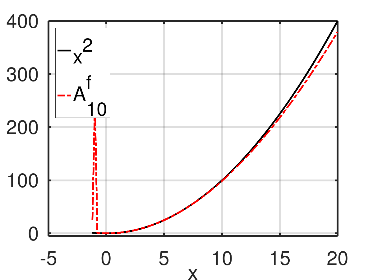
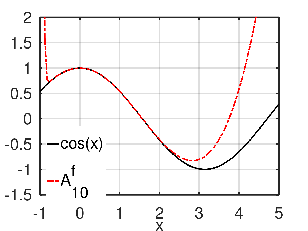
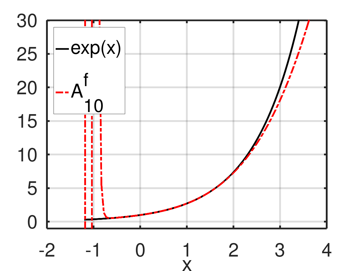
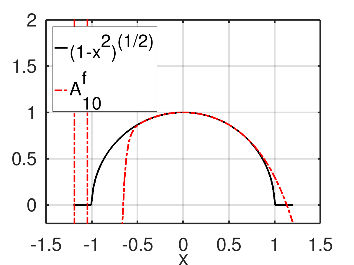
Figure 4: Illustrative examples of approximations based on powers of $g\left(x\right)=\ln\left(x+1\right)$ with 11 terms.

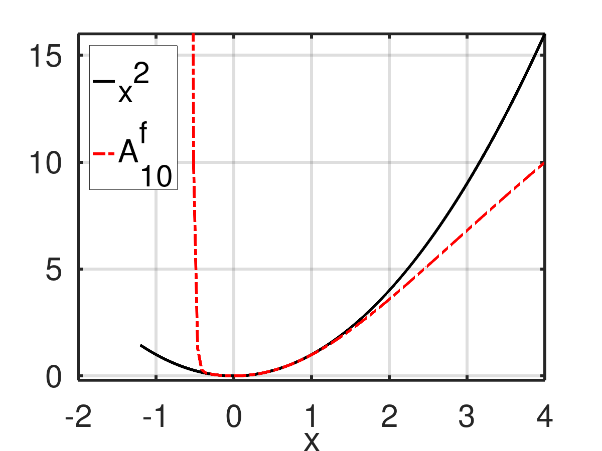
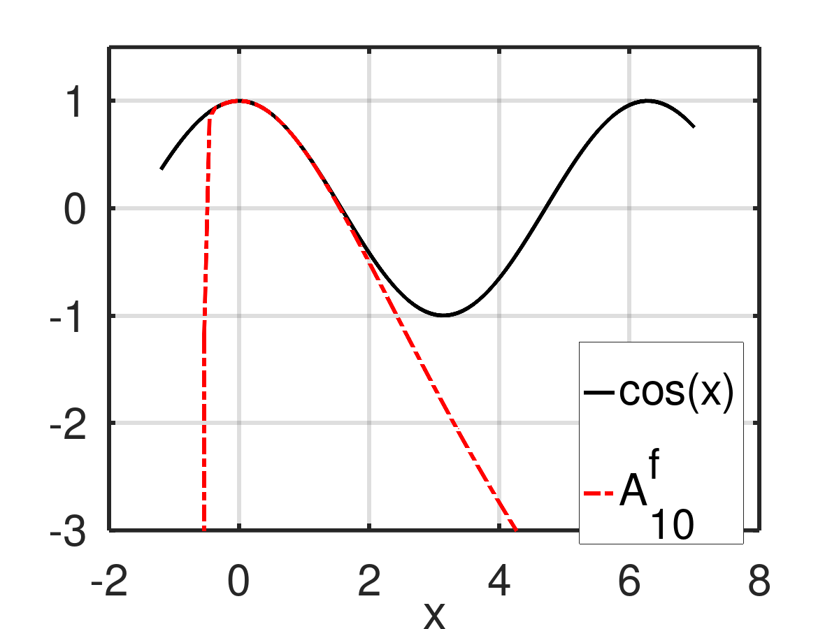
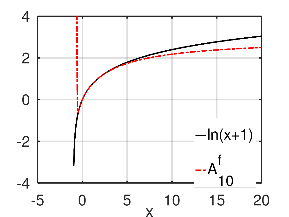
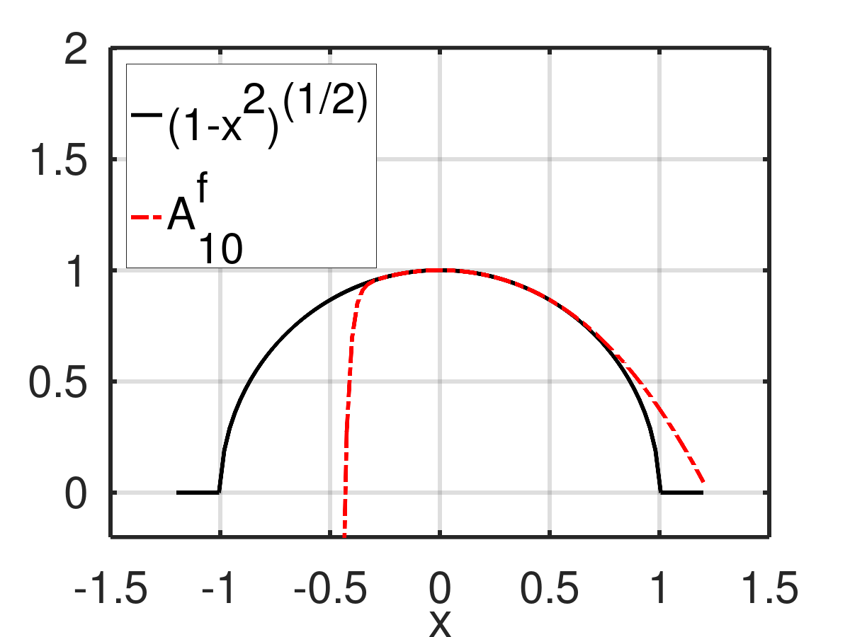
Figure 5: Illustrative examples of approximations based on powers of $g\left(x\right)=x/(x+1)$ with 11 terms.

4.1.3 Expansion into $\sum a_{n}g\left(x^{n}\right),\;g^{\prime}\left(0\right)\neq 0$

An expansion of the form

$$\mathcal{A}^{f}\left(x\right)=\sum_{n=0}^{\infty}a_{n}g\left(x^{n}\right)\;\text{with}\;g^{\prime}\left(0\right)\neq 0$$

is a triangular approximation, which follows from the chain and product differentiation rules. The exception to the “triangular” behavior is the function value for $g\left(0\right)\neq 0$ cases, which requires a dedicated treatment. Writing

$$\mathcal{A}^{f}\left(x\right)=b_{0}+\sum_{n=1}^{\infty}a_{n}g\left(x^{n}\right)\equiv b_{0}+\mathcal{A}_{n>0}^{f}\left(x\right),$$

one can set $b_{0}$ by hand

$$b_{0}=f(0)-\mathcal{A}_{n>0}^{f}\left(0\right),$$ (34)

where the derivative (but not value) matching approximation $\mathcal{A}_{n>0}^{f}$ can be easily constructed (as explained hereunder), since for derivatives ($n>0$) the triangular property holds. Having dealt with the $g\left(0\right)\neq 0$ issue, we assume from now on a more elegant version of the expansion with $g\left(0\right)=0$. Then $b_{0}=f\left(0\right)$ and one has

$$\mathcal{A}^{f}\left(x\right)=f\left(0\right)+\sum_{n=1}^{\infty}a_{n}g\left(x^{n}\right)=f\left(0\right)+\mathcal{A}_{n>0}^{f}\left(x\right).$$ (35)

Independently on the $g\left(0\right)$ value, we are now interested in the derivative matching procedure for $\mathcal{A}_{n>0}^{f}\left(x\right)$. Assuming the analyticity of $g$ in the neighborhood of zero

$$g\left(x\right)=\sum_{n=0}^{\infty}g_{n}x^{n}$$

we proceed with explicit calculations by regrouping the $\mathcal{A}_{n>0}^{f}$ terms by powers of $x$, as expressed in the following table

	$x$	$x^{2}$	$x^{3}$	$x^{4}$	$x^{5}$	$x^{6}$
$a_{1}g\left(x\right)$	$a_{1}g_{1}$	$a_{1}g_{2}$	$a_{1}g_{3}$	$a_{1}g_{4}$	$a_{1}g_{5}$	$a_{1}g_{6}$	$\cdots$
$a_{2}g\left(x^{2}\right)$	$0$	$a_{2}g_{1}$	$0$	$a_{2}g_{2}$	$0$	$a_{2}g_{3}$	$\cdots$
$a_{3}g\left(x^{3}\right)$	$0$	$0$	$a_{3}g_{1}$	$0$	$0$	$a_{3}g_{2}$	$\cdots$
$a_{4}g\left(x^{4}\right)$	$0$	$0$	$0$	$a_{4}g_{1}$	$0$	$0$	$\cdots$
$\vdots$	$\vdots$	$\vdots$	$\vdots$	$\vdots$	$\vdots$	$\vdots$	$\ddots$

.

The factors of $x^{n}$ terms are arranged in columns, rows contain contributions from individual summands of $\mathcal{A}_{n>0}^{f}\left(x\right)$. By plugging different powers of $x$ (shown in different rows) into the argument of $g$ one observes different spacing between non-zero terms. There are no zeros in the first row, in the second row the terms are separated by one zero, in the next row the spacing is two, and so on. It is a version of the sieve of Eratosthenes where the $x^{n}$ monomial is multiplied by all such $a_{i}g_{j}$ where $i$ or $j$ divides $n$ with $i\times j=n$. This is written

$$\mathcal{A}_{n>0}^{f}\left(x\right)=\sum_{n=1}^{\infty}(\sum_{k=1}^{n}\delta_{n\%k,0}a_{k}g_{\frac{n}{k}})x^{n}\equiv\sum_{n=1}^{\infty}(\sum_{k|n}^{n}a_{k}g_{\frac{n}{k}})x^{n}.$$

Assuming also the analyticity of $f$

$$f\left(x\right)=\sum_{n=0}^{\infty}f_{n}x^{n}$$

and the convergence of the approximation $\mathcal{A}^{f}=f$ one can compare the coefficients and write

$$f_{n}=\sum_{k|n}^{n}a_{k}g_{\frac{n}{k}}.$$

Considering $f_{n}$ and $g_{n}$ as fixed, we are interested in finding the inverse relation which allows to expresses $a_{n}$ as their function. The solution is known to be the inverse with respect to the Dirichlet convolution, the latter being defined on two arithmetic function (or sequences) as

$$\left(u*v\right)_{n}=\sum_{k|n}^{n}u_{k}v_{\frac{n}{k}}.$$

The definition of the inverse (denoted by $u^{-1}$) stands

$$\left(u*u^{-1}\right)_{n>0}=\delta_{1,n},$$

where, the existence of $u^{-1}$ requires the assumption $u_{1}\neq 0\neq u_{1}^{-1}$. With $u_{n}\equiv g_{n}$ it implies $g^{\prime}\left(0\right)\neq 0$. Thus we know how to construct the expansion coefficients in (35)

$$a_{n}=\sum_{k|n}\left(g^{-1}\right)_{k}f_{\frac{n}{k}},$$

i.e. the expansion coefficients of $\mathcal{A}^{f}$ involve the Dirichlet inverse of the power-expansion coefficients of $g$ (and vice versa). Each pair of such sequences $\left\{u_{n},\>\left(u^{-1}\right)_{n}\right\}$ can be used to construct two different approximation forms. One of them uses $u_{n}$ to define $g$ (i.e. $g_{n}\equiv u_{n}$) and $\left(u^{-1}\right)_{n}$ to define $a_{n}$, the other does the opposite. Looking in the literature for known examples of Dirichlet inverses we propose two of them.

1. Sequences $u_{n}=1$ and $\left(u^{-1}\right)_{n}=\mu_{n}$ where $\mu_{n}$ denotes the Möbius function. One then gets the two following expansions

   $$\mathcal{A}^{f}\left(x\right)=f\left(0\right)+\sum_{n=1}^{\infty}a_{n}G\left(x^{n}\right),\>a_{n}=\sum_{k|n}f_{\frac{n}{k}},$$ (36)

   where $G$ is the ordinary generating function of the Möbius function

   $$G\left(x\right)\equiv\sum_{n=1}^{\infty}\mu_{n}x^{n}$$ (37)

   and

   $$\mathcal{A}^{f}\left(x\right)=b_{0}+\sum_{n=1}^{\infty}a_{n}\frac{1}{1-x^{n}},\>a_{n}=\sum_{k|n}\mu_{k}f_{\frac{n}{k}},$$ (38)

   with $b_{0}$ given by (34).

2. Sequences

   $$u_{n}=\sin\left(n\pi/2\right)$$

   and

   $$\left(u^{-1}\right)_{n}\equiv\nu_{n}=\begin{cases}\left(-1\right)^{\sum_{p|n}\frac{p+1}{2}}&\text{ for square-free odd }n\\ 0&\text{ else}\end{cases},$$

   where $p$ denotes prime numbers. The proof [30] uses the fact that $u$ represents the Dirichlet-series coefficients of the Dirichlet beta function, which can be expressed as an Euler product and thus easily inverted (with respect to the multiplication). The $u^{-1}$ sequence is then given by the Dirichlet series coefficients of the latter. We chose to present only one of the two expansions

   $$\mathcal{A}^{f}\left(x\right)=f\left(0\right)+\sum_{n=1}^{\infty}a_{n}\frac{x^{n}}{x^{2n}+1},\>a_{n}=\sum_{k|n}\nu_{k}f_{\frac{n}{k}},$$ (39)

   the remaining variant seems not to be very interesting.

In all cases the obvious relation to the characteristic numbers is $f_{m}=c_{m}^{f}/m!$. The shape of the function $G\left(x\right)$ and approximations of the exponential and sine functions with formulas (36), (38) and (39) are shown in Fig. 6.

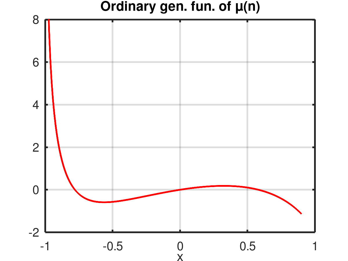
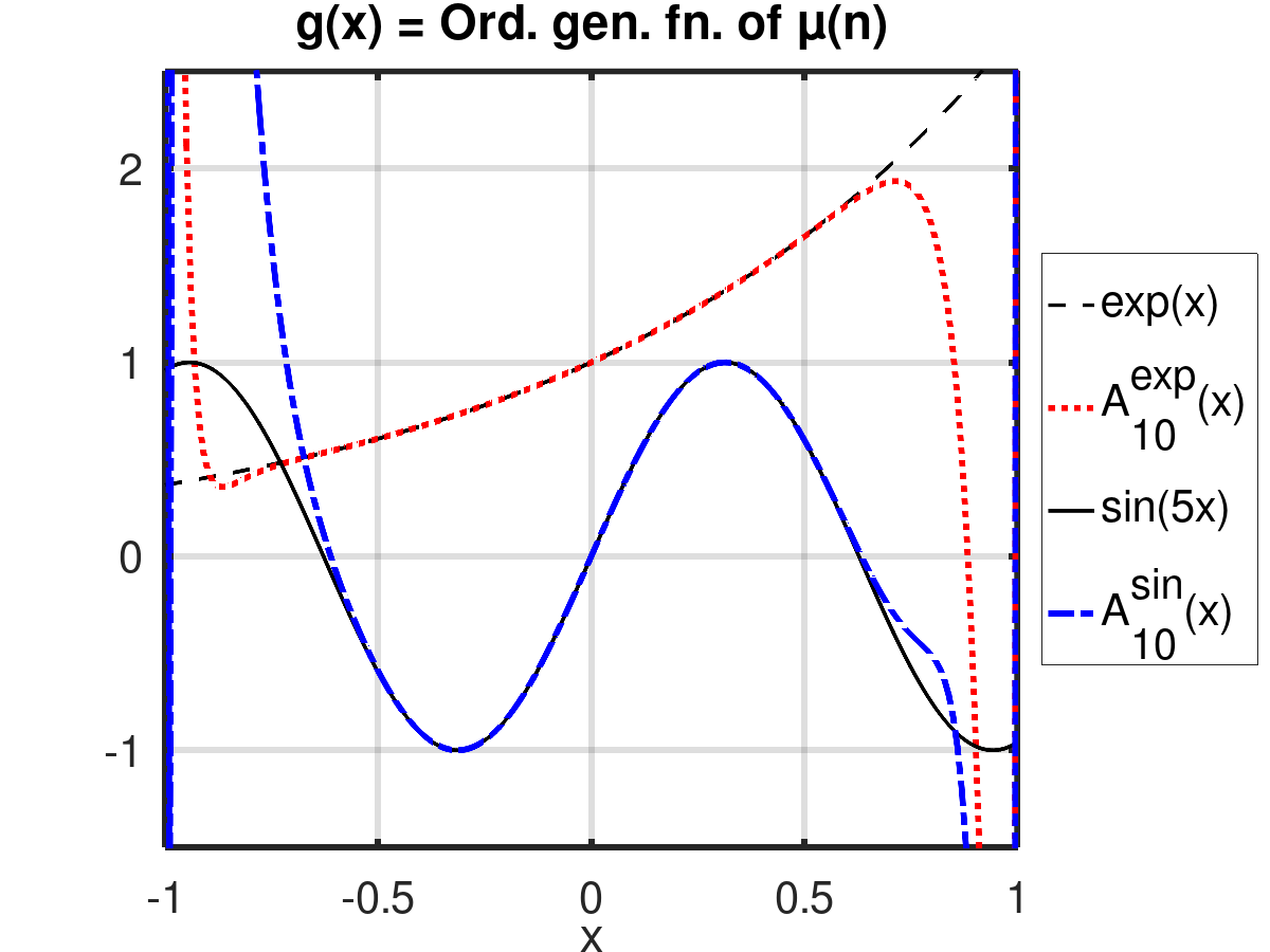
(a)                                           (b)

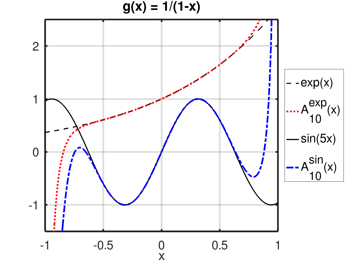
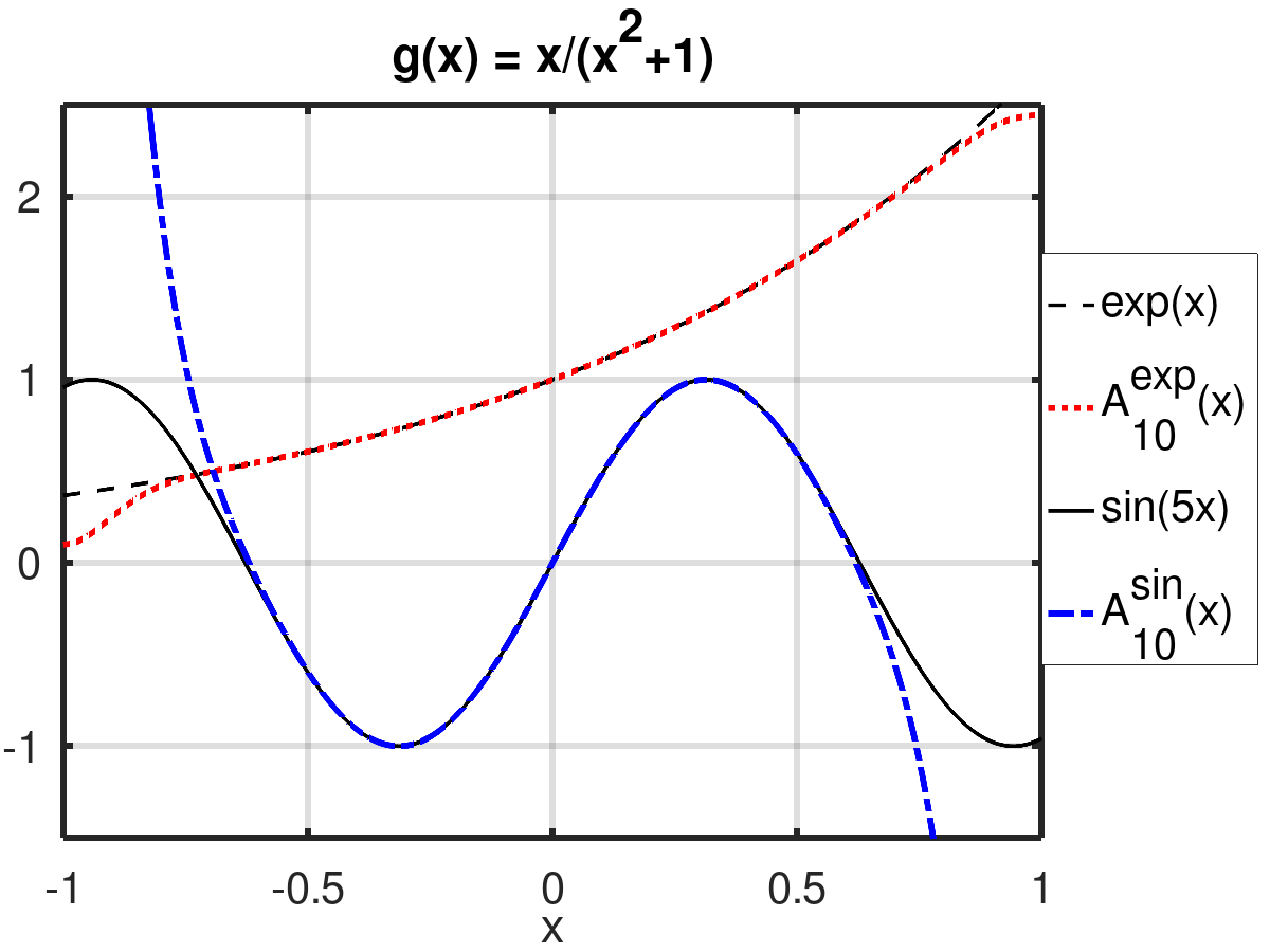
(c)                                           (d)

Figure 6: Ordinary generating function of the Möbius function $G\left(x\right)$ on sub-figure (a) and approximations of $\exp\left(x\right)$ and $\sin\left(5x\right)$ by $\sum_{n}^{10}a_{n}g\left(x^{n}\right)$ with $g(x)=G\left(x\right)$, $g(x)=1/\left(1-x\right)$ and $g(x)=x/\left(x^{2}+1\right)$ on sub-figures b), c) and d) respectively.

The expressions (38) and (39) represent presumably new rational expansions which have singularities situated on the unit circle in the complex plane. The positions of the singularities of (38) correspond to all roots of unity and thus the expression in general diverges for $x=\pm 1$. The singularities of (39) are given by even roots of $-1$, implying the individual summands being well defined for $x=\pm 1$. One can modify the radius of the circle on which the singularities are situated by substitution, the procedure is identical to the one described in Sec. 4.1.2. The domain of convergence $\mathcal{A}^{f}\rightarrow f$ remains an open question, for various elementary functions numerical computations suggest the interval $\left(-1,1\right)$.

4.1.4 Decomposed exponential

Another derivative-matching approximation can be constructed by considering functions which form a closed ring when differentiated

$$\left\{h_{n}\right\}_{n=0}^{N-1}:\quad h_{n}^{{}^{\prime}}=h_{n+1},\;h_{N-1}^{{}^{\prime}}=h_{0},$$

where $N$ is fixed. If $h_{i}$ should play the role of approximation building blocks, their mutual linear independence is suitable. This is however not automatically satisfied (consider the function $\sin(x)$ and the corresponding derivative ring), yet, from the theory of linear differential equations we know the equation

$$h^{\left(N\right)}\left(x\right)=h\left(x\right)$$

allows for $N$ independent solutions. In search of them one can use the fact that the derivative ring as whole (i.e. summed) is derivative-invariant and thus has to be proportional to the exponential function

$$\sum_{n=0}^{N-1}h_{n}\left(x\right)=\alpha\exp\left(x\right),$$

from where the idea to decompose and re-arrange the power expansion of the latter

$$\text{dex}_{\left[N,n\right]}\left(x\right)=\sum_{k=0}^{\infty}\frac{1}{\left(n+kN\right)!}x^{n+kN},\quad 0\leq n<N.$$

Convergence properties of this definition are easy to asses: on the positive real axis all dex function expansions take the form of a sum of positive numbers majorated by the exponential and thus necessarily convergent. Since the convergence domain is a disk around the expansion point, all functions converge in the whole complex plane.

One recovers some known functions

$$\text{dex}_{\left[1,0\right]}\left(x\right)=\exp\left(x\right),\quad\text{dex}_{\left[2,0\right]}\left(x\right)=\cosh\left(x\right),\quad\text{dex}_{\left[2,1\right]}\left(x\right)=\sinh\left(x\right).$$

The dex functions have an important property: only the first in the series $\text{dex}_{\left[N,0\right]}$ is non-zero at zero, all others take by definition a zero value. Because of the ring property (each member becomes its neighbor when differentiated), the differentiation makes the only non-zero member shift along the ring. Thus, considering the value and first $N-1$ derivatives $\left\{c_{n}^{f}\right\}_{n=0}^{N-1}$ of a function, an approximation can be easily constructed as

$$\mathcal{A}_{N}^{f}\left(x\right)=\sum_{n=0}^{N-1}c_{n}^{f}\text{dex}_{\left[N,n\right]}\left(x\right).$$ (40)

The formula can be of course shifted to an arbitrary point by shifting the argument. The expression (40) is to be used as a partial approximation, it suits situations where the number of derivatives to match is fixed and given in advance because going to a higher approximation order means using a different set of the dex functions. The derivatives of (40) are by construction cyclic with period $N$. The convergence to the expanded function can be studied in the limit $N\rightarrow\infty$ where, as a special case, one obtains the Taylor series whose convergence properties are well understood.

As a curiosity, one can define a function (see Fig. 7)

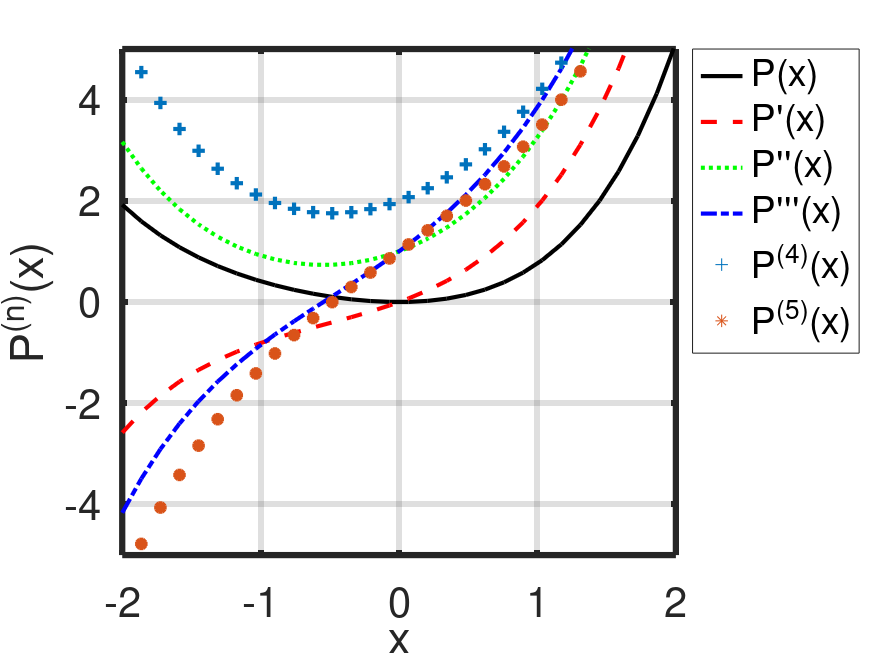
Figure 7: $P\left(x\right)$ function with its derivatives (see the text).

$$P\left(x\right)=\sum_{i=2}^{\infty}\left(\text{dex}_{\left[i,0\right]}-1\right),$$

where the summation is performed in the first index. It is a realization of the sieve of Eratosthenes, one has

$$p\text{ is prime}\Leftrightarrow\frac{d^{p}}{dx^{p}}P\left(x\right)|_{x=0}=1.$$

4.2 Non-linear approximation example

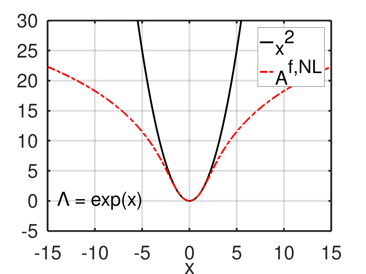
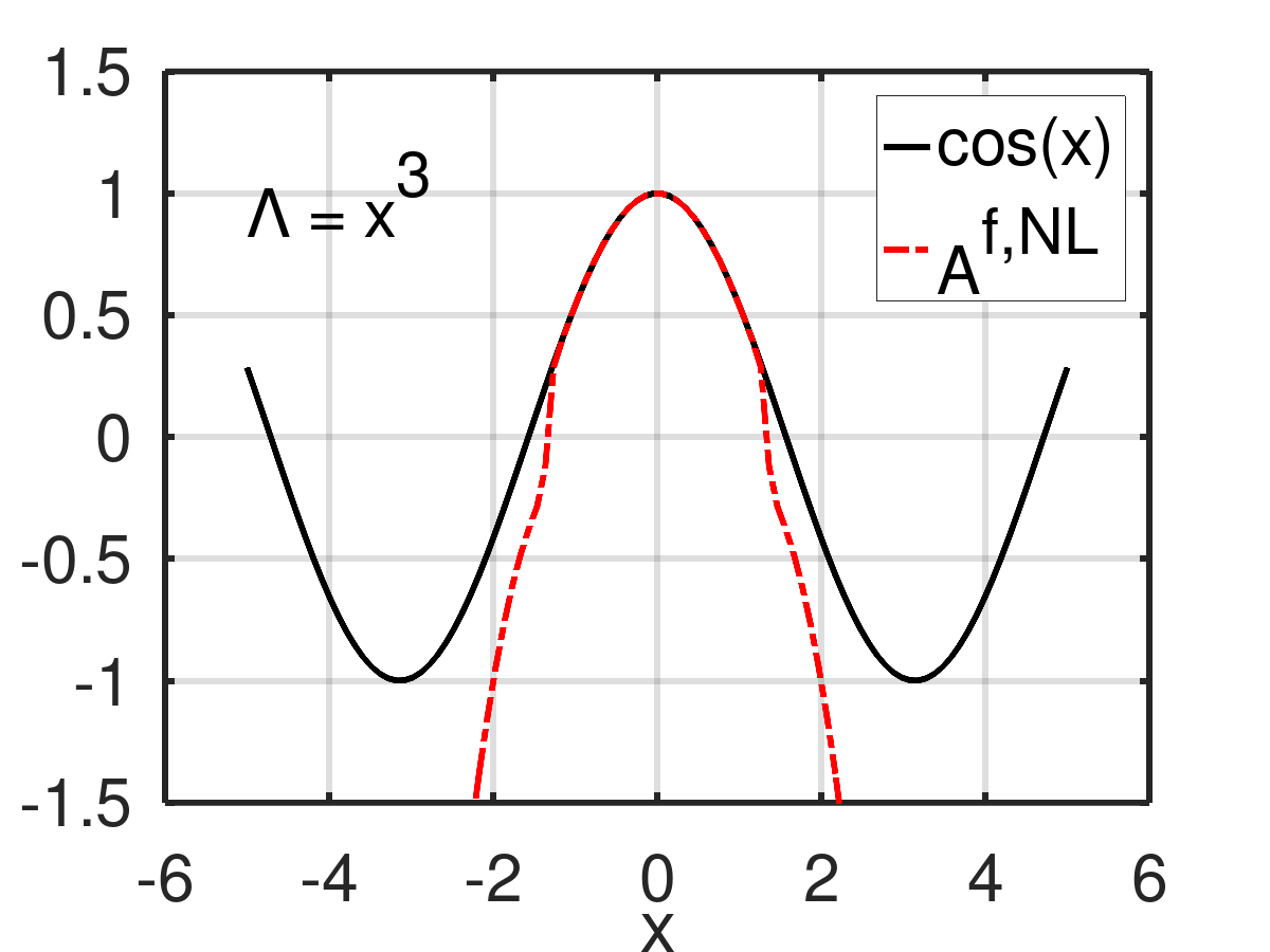
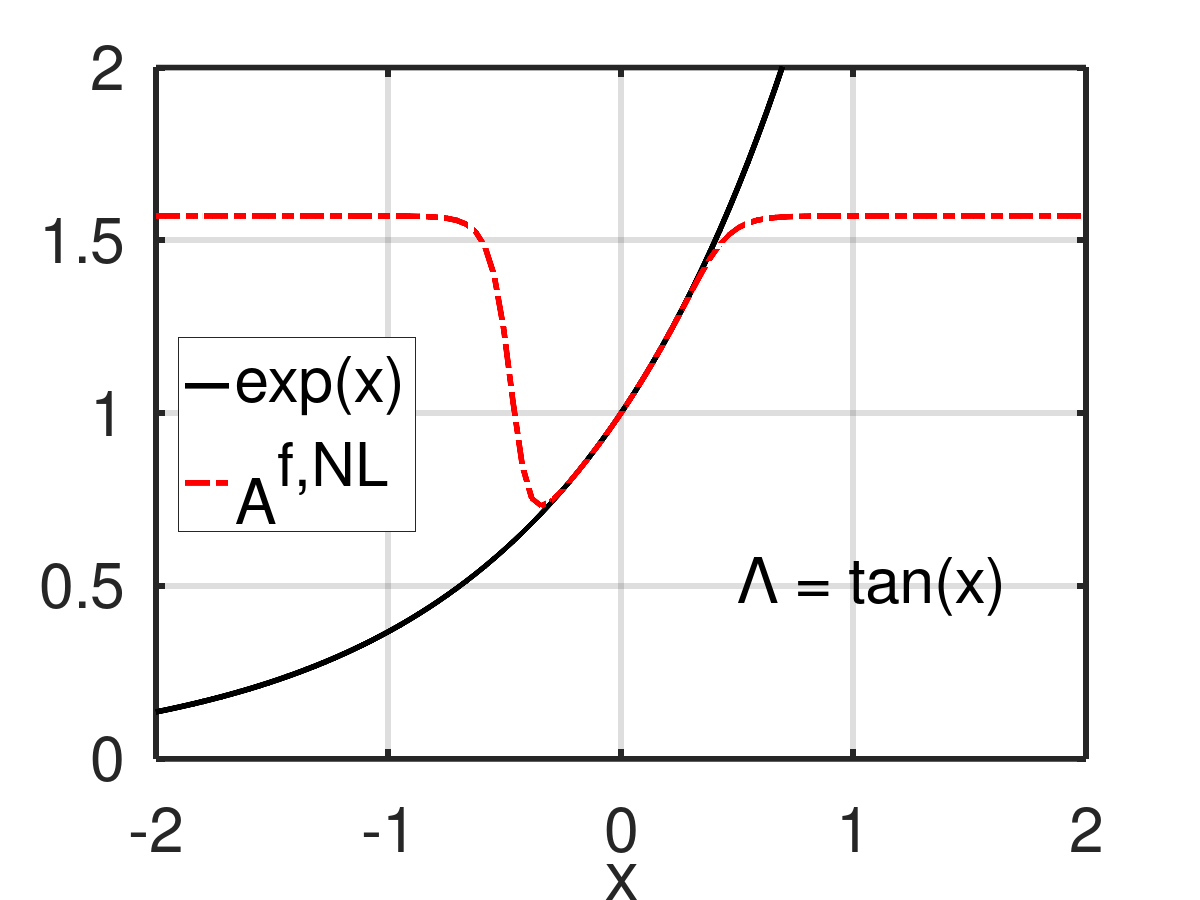
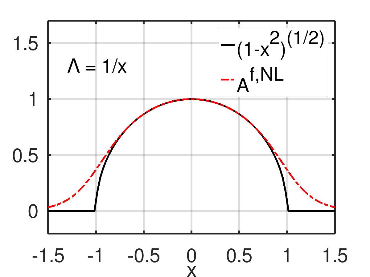
Figure 8: Illustrative examples of the nonlinear approximation (41) with 11 terms.

A simple example of a nonlinear delta approximation can be constructed by matching derivatives of a function $f$ transformed by a different function $\Lambda$

$$\mathcal{C}_{n}=\frac{d^{n}}{dx^{n}}\Lambda\left[\ldots\right]|_{x=0},\quad c_{n}^{f}=\frac{d^{n}\Lambda\left[f\left(x\right)\right]}{dx^{n}}|_{x=0}.$$

We choose by purpose $\Lambda$ to be non-linear so as to imply the non-linearity of the whole functional. The function $f$ is assumed to be strictly monotonic on $\left(a,b\right)$ and $\Lambda$ invertible $\Omega=\Lambda^{-1}$ on its codomain. The approximation is then constructed as

$$\mathcal{A}^{f,NL}\left(x\right)=\Omega\left(\sum_{n=0}^{\infty}a_{n}x^{n}\right)\text{ with }a_{n}=c_{n}^{f}.$$ (41)

The construction is indeed almost trivial, yet it provides us with a valid example of a non-linear functional. Clearly, the convergence properties depend on the convergence behavior of the power expansion which can be analyzed using standard tools known from the Taylor series. This expansion might be of some interest: Setting by hand $a_{n}=\delta_{n,1}$ one has $\mathcal{A}^{\bcancel{f},NL}\left(x\right)=\Omega\left(x\right)$, and so, progressively changing (in some way) the coefficients leads to a progressive change in the function form from $\Omega\left(x\right)$ to $f\left(x\right)$ (assuming the convergence of $\mathcal{A}^{f,NL}$ to $f$)

$$\left\{a_{n}=\delta_{n,1}\right\}\rightarrow\left\{a_{n}=c_{n}^{f}\right\}\Rightarrow\Omega\left(x\right)\rightarrow f\left(x\right).$$

This can be used in a model comparison: if, in some area of science, an established model predicting the behavior $y=\Omega\left(x\right)$ is to be improved by a more precise model, it might be natural to express the prediction of the new model in the form $\Omega\left(\sum_{n=0}^{\infty}a_{n}x^{n}\right)$, so that the deviations of coefficients from zero (from one for $x_{0}$) encode the deviation of the new model from the old one.

Some illustrative examples of the approximation based on formula (41) are shown in Fig. 8.

4.3 Variations on Whittaker–Shannon formula

The Whittaker–Shannon (WS) formula

$$f\left(x\right)=\lim_{t\rightarrow x}\sum_{n=-\infty}^{+\infty}f\left(\frac{n\pi}{T}\right)\frac{\sin\left(Tt-n\pi\right)}{Tt-n\pi},\quad\widetilde{f}\left(\omega\right)=0\text{ for }\left|\omega\right|>T,$$

where $\widetilde{f}\left(\omega\right)$ denotes the Fourier transform assumed continuous on $\left[-T,T\right]$, can be generalized to yield various interpolations and integral-matching approximations (these can be interpreted as interpolations of the primitive function). Such approximations share the argument-scaling feature, i.e. the function is evaluated at different points (or the integral is computed in different limits). In this section we generalize the WS formula to allow for various point distributions, including, for example, distributions on finite intervals concentrated around limit points. We believe this is interesting because the generalization we propose significantly increases the number of use cases (i.e. point configurations). We do not study the effect of the generalization on convergence properties, with this respect we present only numerical observations.

In full generality one can consider a ratio

$$\mathcal{A}^{f,WS}\left(x\right)=\lim_{t\rightarrow x}\sum_{n}a_{n}\frac{\lambda_{n}\left(t\right)}{\omega_{n}\left(t\right)}$$ (42)

where for an infinite set of distinct real numbers $\left\{x_{n}\right\}_{n=-\infty}^{\infty}$ the following is true

$$\lambda_{m}\left(x_{n}\right)=0,\quad\omega_{m}\left(x_{n\neq m}\right)\neq 0,\quad\lim_{t\rightarrow x_{n}}\frac{\lambda_{n}\left(t\right)}{\omega_{n}\left(t\right)}=1.$$

The lower index in $\lambda_{n}$ appears for generality reasons but does not represent a key idea of the construction. A modified version of the above formula

$$\lambda\left(t\right)=\lambda_{0}\left(t\right)=\lambda_{1}\left(t\right)=\lambda_{2}\left(t\right)=\ldots$$

may be more appealing for its simplicity (denoted later on without any index). It is straightforward to see that the approximation property holds

$$a_{n}=c_{n}^{f}\equiv f\left(x_{n}\right),$$

because the individual terms in (42) represent delta functions

$$\lim_{t\rightarrow x_{m}}\frac{\lambda\left(t\right)}{\omega_{n}\left(t\right)}=\delta_{n,m},$$

from which a delta approximation is built. There are no many candidates for $\lambda$ when searching among elementary or commonly used functions: one naturally considers the trigonometric functions, eventually also the Bessel functions, and their modifications.

We propose the function form

$$\mathcal{A}_{N}^{f,WS}\left(x\right)\doteq\sum_{n=-N}^{-N}a_{n}\frac{\mathcal{N}\left(x\right)\sin\left[\pi s\left(x\right)\right]}{s_{n}\left(x-x_{n}\right)},\quad s_{n}\equiv\frac{d}{dx}\left\{\mathcal{N}\left(x\right)\sin\left[\pi s\left(x\right)\right]\right\}|_{x=x_{n}},$$ (43)

where we use $\doteq$ to denote the limit when $x\rightarrow x_{n}\equiv s^{-1}\left(n\right)$, $s\left(x\right)$ is an argument-scaling function invertible on some non-zero interval $I$, $\left\{x_{n}\right\}\subset I$ and $\mathcal{N}\left(x\right)$ is a normalization factor. The latter is important mainly in the neighborhood of limit points, e.g. the function $\sin\left(\pi/x\right)$ behaves chaotically in the proximity of zero while $x\sin\left(\pi/x\right)$ behaves more nicely and this has an impact also on the corresponding sums. As illustrations we provide the following examples

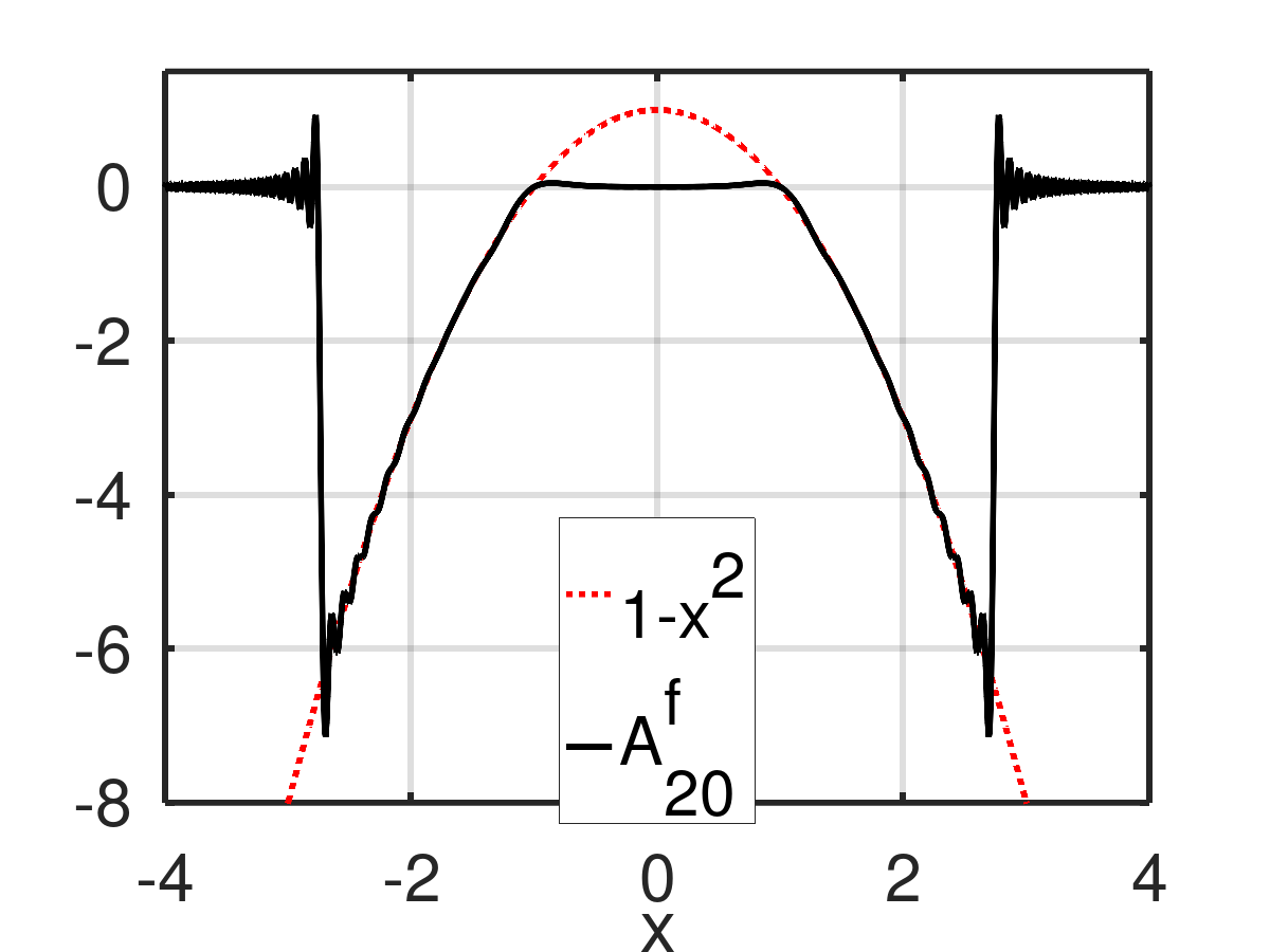
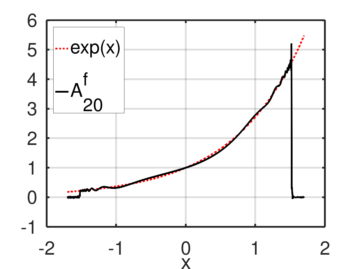
(a)                                                           (b)

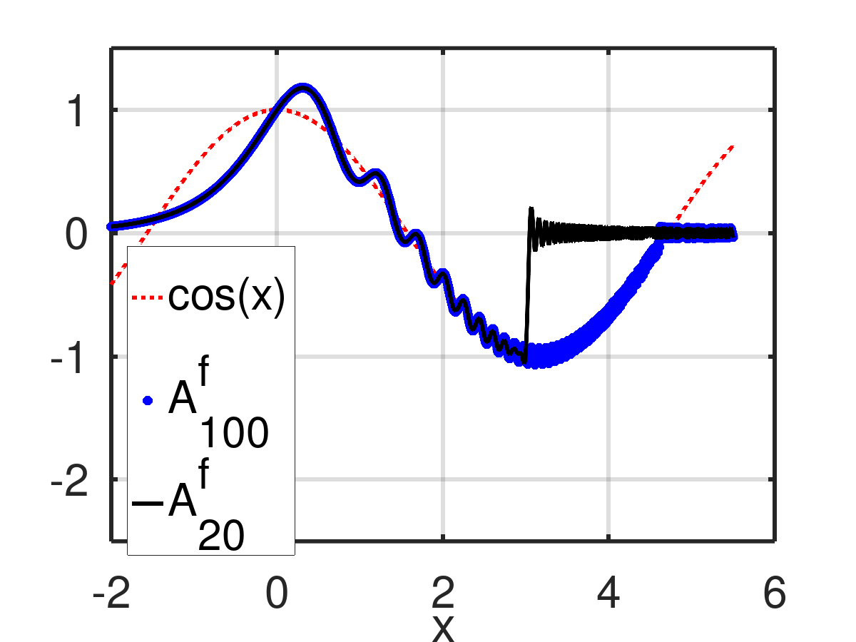
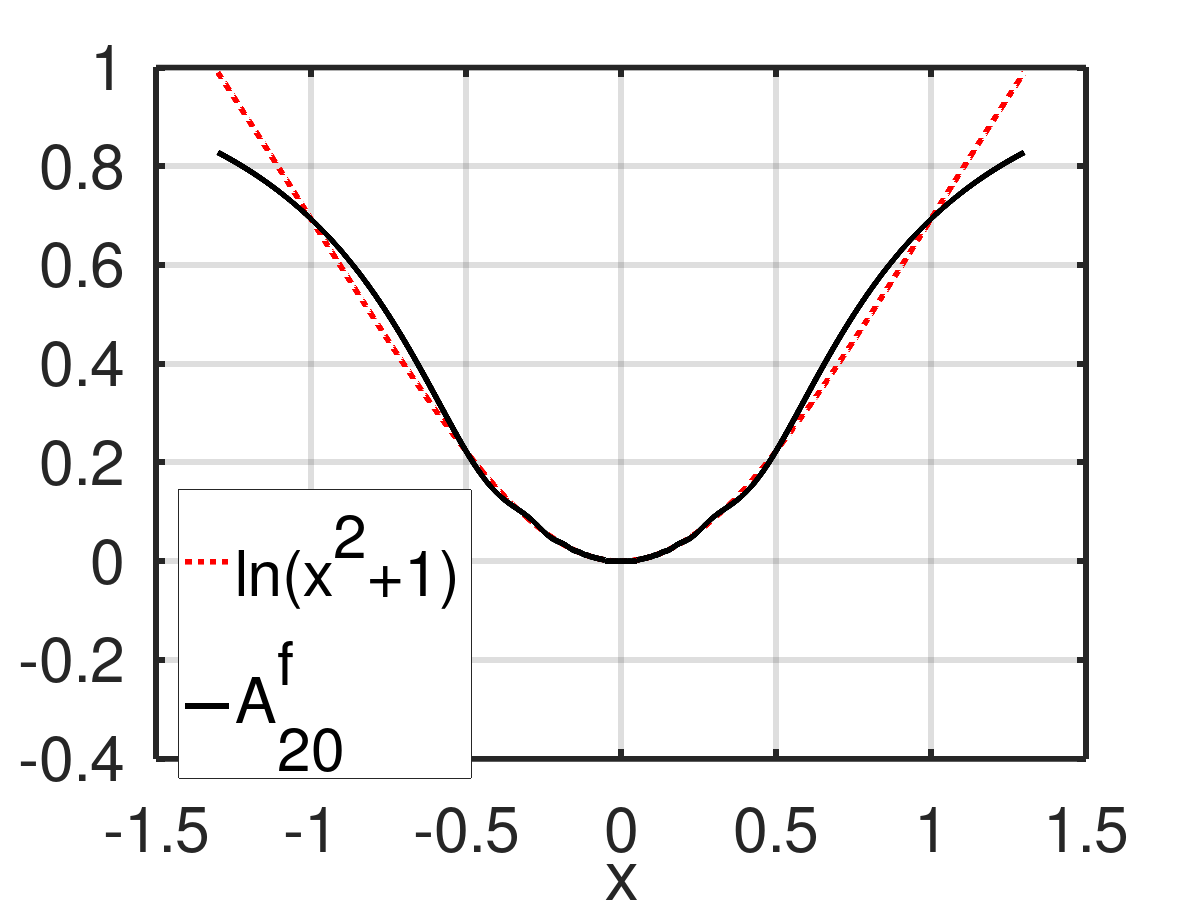
(c)                                                           (d)

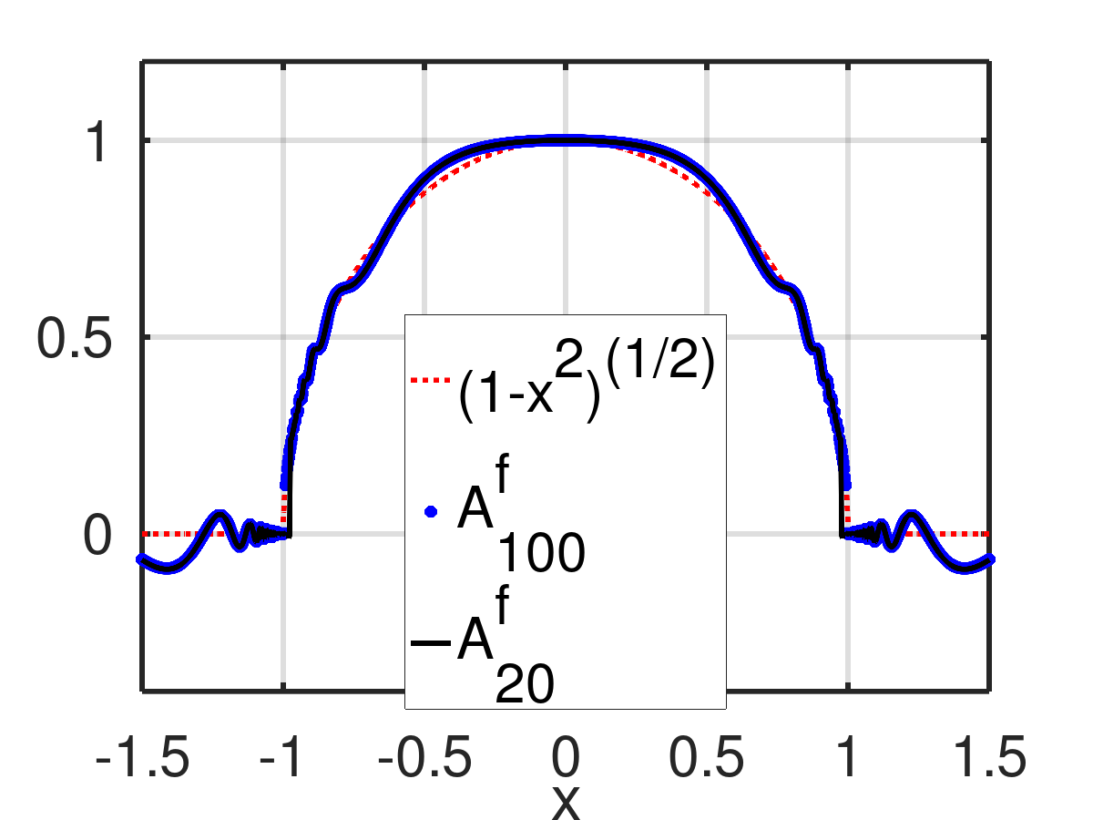
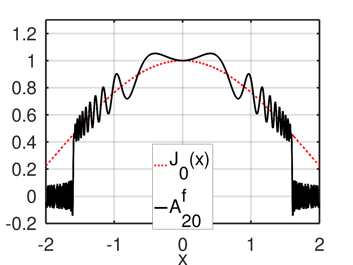
(e)                                                           (f)

Figure 9: Approximations based on a modified WS formula (for details see the text).

• We approximate $f\left(x\right)=1-x^{2}$ using $s(x)=x^{3}$, $x_{n}=\sqrt[3]{n}$, $s_{n}=3\pi n^{2/3}\left(-1\right)^{n}$, $\mathcal{N}\left(x\right)=1$, $N=20$. Because the derivative of $s$ at zero is zero, the term $n=0$ is excluded from the sum. The approximation is show in Fig. 9(a).

• We approximate $f\left(x\right)=e^{x}$ using $s(x)=\tan\left(x\right)$, $x_{n}=\arctan\left(n\right)$, $s_{n}=\pi\left(n^{2}+1\right)\left(-1\right)^{n}$, $\mathcal{N}\left(x\right)=1$, $N=20$. The approximation is show in Fig. 9(b).

• We approximate $f\left(x\right)=\cos\left(x\right)$ using $s(x)=e^{x}$, $x_{n}=\ln\left(n\right)$, $s_{n}=\pi n\left(-1\right)^{n}$, $\mathcal{N}\left(x\right)=1$, $N=20\text{ and }100$. For $x_{n}$ to be well-defined real numbers, only $n>0$ terms are considered in the sum (43). The approximation is show in Fig. 9(c). Increasing the number of terms does not seem to help dumping oscillations and improve the convergence.

• We approximate $f\left(x\right)=\ln\left(x^{2}+1\right)$ using $s(x)=1/x$, $x_{n}=1/n$, $s_{n}=\pi\left(-1\right)^{n+1}$, $\mathcal{N}\left(x\right)=x^{2}$, $N=20$. For $x_{n}$ to be well-defined, the term $n=0$ is excluded from the sum. The approximation is show in Fig. 9(d).

• We approximate $f\left(x\right)=\sqrt{1-x^{2}}$ using $s(x)=x/\left(1-x^{2}\right)$, $x_{n}=2n/(\sqrt{4n^{2}+1}+1)$, $s_{n}=\pi\left(-1\right)^{n}\sqrt{4n^{2}+1}$, $\mathcal{N}\left(x\right)=1-x^{2}$, $N=20\text{ and }100$. The approximation is show in Fig. 9(e).

• We approximate $f\left(x\right)=J_{0}\left(x\right)$ using $s(x)=xe^{x^{2}}$, $x_{n}=\text{sgn}\left(n\right)\sqrt{W\left(2n^{2}\right)/2}$, $\mathcal{N}\left(x\right)=1$, $N=20$, where $J_{0}$ is the Bessel function, sgn is the sign function, $W$ is the principal branch of the Lambert W function and the expression for $s_{n}$ is not shown (because of its complexity). The approximation is depicted in Fig. 9(f).

The general observations for the studied cases are

• Functions $\mathcal{A}_{N}^{f,WS}$ seem to converge (not necessarily to $f$) and thus approximate $f$ at least to some extent. In the case (a), the missing interpolation point $x_{0}=0$ situated in between other points causes the approximation to deviate importantly in its proximity.

• It is difficult to assert about the convergence $\mathcal{A}_{N}^{f,WS}\rightarrow f$. The cases (c) and (e) suggest that (for some functions) a higher approximation order does not improve the convergence. Increasing $N$ however extends the range $(x_{n}^{\text{min}},x_{n}^{\text{max}})$ and thus enlarges the interval on which $\mathcal{A}_{N}^{f,WS}$ provides some (at least rough) approximation of $f$.

• In situations where $x_{n}$ points concentrate on the edges of the $(x_{n}^{\text{min}},x_{n}^{\text{max}})$ interval, a Gibbs-like phenomenon is observed there.

For integral matching the set of characteristic numbers is given by

$$c_{n}^{f}=\int_{a}^{x_{n}}f\left(x\right)dx.$$

One first needs to choose appropriate building blocs for the interpolation function $\mathcal{A}^{f,\text{int.}}$ so as to satisfy

$$A^{f,\text{int.}}\left(a\right)=0$$

and thus ensure

$$\left[\mathcal{A}^{f,\text{int.}}\left(x\right)\right]_{a}^{x_{n}}\equiv\mathcal{A}^{f,\text{int.}}\left(x_{n}\right)-\mathcal{A}^{f,\text{int.}}\left(a\right)=\mathcal{A}^{f,\text{int.}}\left(x_{n}\right)$$

Interpreting $A^{f,\text{int.}}$ as the primitive function

$$\mathcal{A}^{f,\text{int.}}\left(x_{n}\right)=F\left(x_{n}\right)=c_{n}^{f},\quad F^{\prime}=f,$$

the integral matching approximation $A^{f,\int}$ of $f$ is written as

$$\mathcal{A}^{f,\int}\left(x\right)=\left[\mathcal{A}^{f,\text{int.}}\left(x\right)\right]^{\prime}.$$

The fact that the differentiation often generates oscillation [31] seems to be a drawback of this method. The latter suggests that maybe an opposite procedure should be performed: differentiate $f$ several times, interpolate the resulting higher order derivative and then apply (to the approximation) a repeated integration, which is known to have (in general) a smoothing effect.

5 Summary, conclusion, outlook

The text interprets function approximation in a very general framework of matching the characteristic numbers given by a (possibly non-linear) functional action on the approximated function. To our knowledge all existing approximations fit into this construction, we reviewed some of them. Further, we proposed several new expansions mostly exploiting the Taylor-like derivative-matching approach, but we also numerically investigated some extensions of the Whittaker–Shannon interpolation formula.

Maybe the most interesting results are the three presumably new rational expansions (33), (38) and (39), which posses interesting properties, such as an efficient evaluation on a computer, an integrability within elementary functions or coefficients which can be easily calculated order-by-order (unlike for the Padé approximant). In addition, with the differentiation being linear, one can consider an approximation by linearly combining them. Unfortunately, one cannot fully control the positions of singularities since these are given by construction.

The text also opens the possibility to further investigate new approximations by focusing on other special cases of the Bell polynomial arguments (Sec. 4.1.2) or other pairs of mutually Dirichlet-inverse arithmetic functions (Sec. 4.1.3).

We did not provide detailed motivations to all new expansions. Yet, several of them are constructed using a general function $g$ and thus our results represent a large family of possible approximations. A number of them can be well suited for some specific purposes the author may not be aware of, yet we have many examples of mathematical methods whose usefulness was seen only after their development.

In the present article we focused almost entirely on the approximation property as we understand it, and did not make conclusions concerning the convergence, unless such conclusions could be simply related to known cases (the Taylor series). The convergence issues being usually technically difficult, the text can be understood as a starting point for studying them (for the various new expansions we proposed) in the future.

References

- [1] D. V. Widder. A generalization of taylor’s series. Trans. Am. Math. Soc, 30(1):126–154, 1928.
- [2] P.J. Davis. Interpolation and Approximation. Dover Books on Mathematics. Dover Publications, 1975.
- [3] Mohammad Masjed-Jamei. On constructing new interpolation formulas using linear operators and an operator type of quadrature rules. Journal of Computational and Applied Mathematics, 216(2):307–318, July 2008.
- [4] Mohammad Masjed-Jamei. On constructing new expansions of functions using linear operators. Journal of Computational and Applied Mathematics, 234:365–374, 05 2010.
- [5] Mohammad Masjed-Jamei, Zahra Moalemi, Ivan Area, and Juan Nieto. A new type of taylor series expansion. Journal of Inequalities and Applications, 2018, 05 2018.
- [6] C. G. Neumann. Die theorie der Besselschen funktionen. B.G. Teubner Verlag, Leipzig, 1867.
- [7] G. Watson. Treatise on the Theory of Bessel Functions. Cambridge University Press, 1922.
- [8] Vladislav V. Kravchenko, Sergii M. Torba, and Raúl Castillo-Pérez. A neumann series of bessel functions representation for solutions of perturbed bessel equations. Applicable Analysis, 97(5):677–704, 2018.
- [9] Vladislav V. Kravchenko, Luis J. Navarro, and Sergii M. Torba. Representation of solutions to the one-dimensional schrödinger equation in terms of neumann series of bessel functions. Applied Mathematics and Computation, 314:173–192, 2017.
- [10] George A Baker, George A Baker Jr, George Baker, Peter Graves-Morris, and Susan S Baker. Pade Approximants: Encyclopedia of Mathematics and It’s Applications, Vol. 59 George A. Baker, Jr., Peter Graves-Morris, volume 59. Cambridge University Press, 1996.
- [11] Hiroaki S. Yamada and Kensuke S. Ikeda. A numerical test of pade approximation for some functions with singularity. https://arxiv.org/abs/1308.4453, 2013.
- [12] Alexander I. Aptekarev and Maxim L. Yattselev. Padé approximants for functions with branch points - strong asymptotics of nuttall-stahl polynomials. Acta Mathematica, 215(2):217 – 280, 2015.
- [13] P. L. Butzer, K. Schmidt, E.L. Stark, and L. Vogt. Central factorial numbers; their main properties and some applications. Numerical Functional Analysis and Optimization, 10(5-6):419–488, 1989.
- [14] Feng Qi, Guo-Sheng Wu, and Bai-Ni Guo. An alternative proof of a closed formula for central factorial numbers of the second kind. Turkish Journal of Analysis and Number Theory, 7(2):56–58, 2019.
- [15] Konrad Schmüdgen. The Moment problem. Graduate texts in mathematics, 277. Springer International, Cham, Switzerland, 2017 - 2017.
- [16] R Askey, I.J Schoenberg, and A Sharma. Hausdorff’s moment problem and expansions in legendre polynomials. Journal of Mathematical Analysis and Applications, 86(1):237–245, 1982.
- [17] G Talenti. Recovering a function from a finite number of moments. Inverse Problems, 3(3):501–517, aug 1987.
- [18] A. O. Savchenko. Matrix of moments of the Legendre polynomials and its application to problems of electrostatics. Computational Mathematics and Mathematical Physics, 57(1):175–187, January 2017.
- [19] Parminder Kaur, Husanbir Singh Pannu, and Avleen Kaur Malhi. Comprehensive study of continuous orthogonal moments - a systematic review. ACM Comput. Surv., 52(4), August 2019.
- [20] V. I. Krylov. Approximate calculation of integrals. Macmillan, New York, 1962.
- [21] C. Jordan. Calculus of finite differences. Chelsea, New York, 1965.
- [22] L.J Mordell. Expansion of a function in a series of bernoulli polynomials, and some other polynomials. Journal of Mathematical Analysis and Applications, 15(1):132–140, 1966.
- [23] Mohammad Masjed-Jamei, Gradimir V. Milovanović, and Z. Moalemi. A generalization of divided differences and applications. Filomat, 33:193–210, 2019.
- [24] G. Pick. Über die Beschränkungen analytischer Funktionen, welche durch vorgegebene Funktionswerte bewirkt werden. Math. Ann., 77:7–23, 1915.
- [25] Adem Sahin. Inverse and factorization of triangular toeplitz matrices. Miskolc Mathematical Notes, 19:527, 01 2018.
- [26] Feng Qi, Da-Wei Niu, Dongkyu Lim, and Yong-Hong Yao. Special values of the bell polynomials of the second kind for some sequences and functions. Journal of Mathematical Analysis and Applications, 491(2):124382, 2020.
- [27] Feng Qi and Bai-Ni Guo. Explicit formulas for special values of the bell polynomials of the second kind and for the euler numbers and polynomials. Mediterranean Journal of Mathematics, 14:14 pages, 05 2017.
- [28] Weiping Wang and Tianming Wang. General identities on bell polynomials. Computers & Mathematics with Applications, 58(1):104–118, 2009.
- [29] F. T. Howard. A special class of bell polynomials. Mathematics of Computation, 35:977–989, 1980.
- [30] Gergö Nemes. Dirichlet inverse for . https://math.stackexchange.com/questions/4306673/dirichlet-inverse-for-left-1-0-1-0-1-0-1-0-1-0-1-0-ldots-right, Nov 2021. Posted as user "Gary".
- [31] MV Berry. Universal oscillations of high derivatives. Proceedings of the Royal Society A: Mathematical, Physical and Engineering Sciences, 461(2058):1735–1751, 2005.