Wave dynamic on multidimensional tropical series

Abstract.

We define multidimensional tropical series, i.e. piecewise linear function which are tropical polynomials locally but may have infinite number of monomials. Tropical series appeared in the study of the growth of pluriharmonic functions. However our motivation originated in sandpile models where certain wave dynamic governs the behaviour of sand and exhibits a power law (so far only experimental evidence). In this paper we lay background for tropical series and corresponding tropical analytical hypersurfaces in the multidimensional setting. The main object of study is $\Omega$-tropical series where $\Omega$ is a compact convex domain which can be thought of the region of convergence of such a series.

Our main theorem is that the sandpile dynamic producing an $\Omega$-tropical analytical hypersurface passing through a given finite number of points can always be slightly perturbed such that the intermediate $\Omega$-tropical analytical hypersurfaces have only mild singularities.

In this article we develop the theory of tropical series on domains in $\mathbb{R}^{n}$ and prove statements for our future paper about sandpiles (see [8], [6] for sandpiles in two-dimensional case). Our initial motivation was [4] where it was experimentally observed that tropical curves appear in two-dimensional sandpile models and behave nicely when we add more sand. In the subsequent papers we establish similar results for higher dimensional tropical surfaces.

We experimentally found, [7], that the dynamic generated by shrinking operators on the space of tropical series in two-dimensional case obeys power law. Namely, the distribution of the area of an avalanche (a direct analog of that for sandpiles) in this model has the density function of the type $p(x)=cx^{\alpha}$. To the best of our knowledge, this simple geometric dynamic is the only model, among the ways to obtain power laws in a simulation, which produces a continuous random variable. Our shrinking operators appear in works of C. Vafa under the name of “breathing mode”, see [19].

Tropical series appeared in the study of the growth of plurisubharmonic functions [10],[11], Section 5, and [1]. Tropical series in one variable can be studied in the context of ultradiscretization of differential equations, see [18] and references therein. See also [5],[14],[12] for tropical Nevalinna theory. One-dimensional tropical series were used in automata-theory in [13], [15].

For a general introduction to tropical geometry, see [3], [16], or [2]. This paper extends the results of [9] to higher dimensions.

Acknowledgments. We thank Andrea Sportiello for sharing his insights on perturbative regimes of the Abelian sandpile model which was the starting point of our work on sandpiles (first, in two-dimensional case, now in all dimensions). Research is supported by the Russian Science Foundation grant 20-71-00007.

1. Tropical series

Recall that a tropical Laurent polynomial (later just tropical polynomial) $f$ on $U\subset\mathbb{R}^{n}$ in $n$ variables is a function $f:U\to\mathbb{R}$ which can be written as

$$f(z)=\min_{q\in\mathcal{A}}(z\cdot q+a_{q}),a_{q}\in\mathbb{R},z\in U$$ (1.1)

where $\mathcal{A}$ is a finite subset of $\mathbb{Z}^{n}$. Each point $q\in\mathcal{A},q=(q_{1},q_{2},\dots,q_{n})$ corresponds to a tropical monomial $q_{1}z_{1}+q_{2}z_{2}+\dots q_{n}z_{n}+a_{q},z=(z_{1},z_{2},\dots,z_{n})\in U$, the number $a_{q}$ is called the coefficient of the monomial corresponding to the point $q\in\mathcal{A}$. The locus of the points in $U^{\circ}$ where a tropical polynomial $f$ is not smooth is called a tropical hypersurface (see [16]). We denote this locus by $C(f)\subset U^{\circ}$.

The subgraph of $f:U\to\mathbb{R}$ is a convex polyhedron and the projection to $U$ of the faces of dimension $n-1$ of the graph of $f$ constitute $C(f)$. So, $C(f)$ is exactly the set of points $z\in U$ such that there exist $q_{1},q_{2}\in\mathcal{A}$ such that $f(z)=q_{1}\cdot z+a_{q_{1}}=q_{2}\cdot z+a_{q_{2}}$.

Definition 1.2.

Let $U\subset\mathbb{R}^{n},U^{\circ}\neq\varnothing$. A continuous function $f:U\to\mathbb{R}$ is called a tropical series if for each $z_{0}\in U^{\circ}$ there exists an open neighborhood $W\subset U$ of $z_{0}$ such that $f|_{W}$ is a tropical polynomial.

Definition 1.3 (Cf. Definition 2.1).

A tropical analytic hypersurface in $U$ is the locus of non-linearity of a tropical series $f$ on $U^{\circ}$. We denote this hypersurface by $C(f)\subset U^{\circ}$. Equivalently, $C(f)$ is the set of points where $f$ is not smooth.

Example 1.4.

Tropical $\Theta$-divisors [17] are tropical analytic curves in $\mathbb{R}^{2}$. Another simple example is the union of all horizontal and vertical lines passing through lattice points in $\mathbb{R}^{2}$, i.e. the set

$$C=\bigcup\limits_{k\in\mathbb{Z}}\{(k,y)|y\in\mathbb{R}\}\cup\{(x,k)|x\in\mathbb{R}\}.$$

The following example illustrates that a tropical series on $\Omega^{\circ}$ in general cannot be extended to $\partial\Omega$.

Example 1.5.

Consider a tropical analytic curve $C$ in the square $(0,1]\times[0,1]$, presented as

$$C=\bigcup_{n\in\mathbb{N}}\Bigl{\{}\big{(}1/n,y\big{)}|y\in[0,1]\Bigl{\}}\cup\Bigl{\{}\big{(}x,1/2\big{)}|x\in(0,1]\Bigl{\}}.$$

For all tropical series $f$ with $C(f)=C$, the sequence of values of $f(x,y)$ tends to $-\infty$ as $x\to 0$, hence it cannot be extended to $\partial((0,1]\times[0,1])$.

Question 1.6.

What can we say about a set of points in $\partial\Omega$ where a tropical series from $\Omega^{\circ}$ can be extended? Can it have an infinite number of connected components?

Tropical series on non-convex domains exhibit the behaviour as in the following example.

Example 1.7.

The function $f(x,y)=\min(3,x+[y])$ is a tropical series on the following $U$:

$$U=(U_{1}\cup U_{2})^{\circ},U_{1}=\big{(}[0,5]\times[0,1]\big{)}\cup\big{(}[4,5]\times[1,2]\big{)},U_{2}=\big{(}[0,5]\times[2,3]\big{)}\cup\big{(}[4,5]\times[1,2]\big{)},$$

but $f|_{U_{1}^{\circ}}=\min(3,x),f|_{U_{2}^{\circ}}=\min(3,x+2)$ and the monomial $x$ appears with different coefficients $0,2$ in the different parts of $U$.

That is why we further consider tropical series only on convex domains.

2. $\Omega$-tropical series

Definition 2.1.

An $\Omega$-tropical series on a convex closed set $\Omega\subset\mathbb{R}^{n}$ with non-empty interiour is a function $f:\Omega\to\mathbb{R}_{\geq 0}$, $f|_{\partial\Omega}=0$, such that

$$f(z)=\inf\limits_{q\in\mathcal{A}}(q\cdot z+c_{q}),c_{q}\in\mathbb{R},$$ (2.2)

and $\mathcal{A}\subset\mathbb{Z}^{n}$ is not necessary finite. An $\Omega$-tropical analytic hypersurface $C(f)$ on $\Omega^{\circ}$ is the corner locus (i.e. the set of non-smooth points) of an $\Omega$-tropical series $f$ on $\Omega^{\circ}$.

Question 2.3.

An $\Omega$-tropical series can be thought of an analog of a series $f_{t}(z)=\sum_{q\in\mathcal{A}}t^{c_{q}}z^{q}$ with $t\in\mathbb{R}_{>0}$ very small. Is is true that $\Omega^{\circ}$ is the limit of the images of the region of convergence of $f_{t}$ under the map $\log_{t}:z\to(\log_{t}|z_{1}|,\dots,\log_{t}|z_{n}|)$, and the corresponding $\Omega$-tropical analytic hypersurface is the limit of the images of $\{f_{t}(z)=0\}$ under $\log_{t}|\cdot|$ when $t\to 0$? Locally it is true, but it is not clear what can happen near $\partial\Omega$.

Lemma 2.4.

Let $U\subset\mathbb{R}^{n}$ be an open set and $K\subset U$ be a compact set. For any $A>0$ the set

$$\big{\{}q\in\mathbb{Z}^{n}|\exists a_{q}\in\mathbb{R},(q\cdot z+a_{q})|_{U}\geq 0,\exists z_{0}\in K,(q\cdot z_{0}+a_{q})\leq A\big{\}},$$

i.e. the set of monomials, which potentially can contribute on $K$ to an $\Omega$-tropical function $f$ with $\max_{K}f\leq A$, is finite.

Proof.

If $U=\mathbb{R}^{n}$, this set contains only $0\in\mathbb{Z}^{n}$. So, let $R>0$ denote the distance between $K$ and $\mathbb{R}^{n}\setminus U$. Then $(q\cdot z+a_{q})|_{K}\geq R\cdot|q|$ for any $q\in\mathbb{Z}^{n}\setminus 0$ and $a_{q}$ such that $(q\cdot z+a_{q})|_{U}\geq 0$. Therefore, $|q|\leq A/R$ for all $q\in\mathcal{M}.$ ∎

Lemma 2.5.

In the definition of an $\Omega$-tropical series $f$, (2.2), we can replace “$\inf$” by “$\min$”, i.e. at every point $z\in\Omega^{\circ}$ we have

$$\inf\limits_{q\in\mathcal{A}}(q\cdot z+c_{q})=\min\limits_{q\in\mathcal{A}}(q\cdot z+c_{q}).$$

Proof.

Suppose that for a point $z_{0}\in\Omega^{\circ}$ and for each $q\in\mathcal{A}$ the value of the monomial $c_{q}+q\cdot z$ is distinct from the value of the infimum

$$\inf\limits_{q\in\mathcal{A}}(q\cdot z_{0}+c_{q}).$$

Thus, there exists $\text{C}>0$ such that we have $c_{q}+q\cdot z_{0}<\text{C}$ for infinite number of monomials $p\in\mathcal{A}$. Since $(c_{q}+q\cdot z)|_{\Omega}\geq 0$ for all $q\in\mathcal{A}$, applying Lemma 2.4 yields a contradiction. ∎

At a point on $\partial\Omega$ where there is no tangent plane with a rational slope we actually have to take the infimum, cf. the proof of Lemma 3.5.

Applying Lemma 2.4 for small compact neighbors of points we obtain the following result.

Corollary 2.6.

An $\Omega$-tropical series (Definition 2.1) is a tropical series on $\Omega$ in the sense of Definition 1.2.

Lemma 2.7.

Suppose that $\Omega$ is a convex set, and a continuous function $f:\Omega\to\mathbb{R}$ satisfies two conditions: 1) $f|_{\Omega^{\circ}}$ is a tropical series, and 2) $f|_{\partial\Omega}=0$. Then $f$ is an $\Omega$-tropical series (Definition 2.1).

Proof.

Let $f|_{U}=q\cdot z+c_{q}$ for an open $U\subset\Omega^{\circ}$. It follows from convexity of $\Omega$ and local concavity of $f$ that $f(z)\leq q\cdot z+c_{q}$ on $\Omega$. Define

$$g(z)=\inf\{q\cdot z+c_{q}|(q,c_{q}),\exists\text{ open }U\subset\Omega^{\circ},f(z)|_{U}=q\cdot z+c_{q}\}.$$

On $\Omega^{\circ}$ this infimum is actually a minimum and $f=g$. We only need to prove that $g|_{\partial\Omega}=0$. Suppose the contrary. Let $g(x)=A>0,x\in\partial\Omega$. Consider a sequence of $x_{i}\to x,x_{i}\in\Omega^{\circ}$ then $g(x_{i})=f(x_{i})\to 0$. But we have that $g(x_{i}-(x-x_{i}))\leq g(x_{i})-(g(x)-g(x_{i}))$ because $g$ is the infimum of a set of linear functions. But we may choose $x_{i}$ such that $2x_{i}-x\in\Omega^{\circ}$ and $2g(x_{i})-A<0$ which brings a contradiction. ∎

3. Tropical distance function

Each domain $\Omega$ admits the trivial tropical series, which is everywhere equal to zero, its tropical analytic hypersurface is empty.

Not all convex closed subsets $\Omega\subset\mathbb{R}^{n}$ admit a non-tropical $\Omega$-tropical series, e.g. $\mathbb{R}^{n}$, half-space with the boundary of non-rational slope, etc.

Definition 3.1.

Let $\Omega\subset\mathbb{R}^{n}$. For $q\in\mathbb{Z}^{n}$ denote by $c_{q}\in\mathbb{R}\cup\{-\infty\}$ the infimum of $z\cdot q$ over $z\in\Omega$. Let $\mathcal{A}_{\Omega}$ be the set of $q$ with $c_{q}\neq-\infty.$ Note that if $\Omega$ is bounded, then $\mathcal{A}_{\Omega}=\mathbb{Z}^{n}$. For each $q\in\mathcal{A}_{\Omega}$ we define

$$l^{q}_{\Omega}(z)=z\cdot q-c_{q}.$$

Note that $l^{q}_{\Omega}$ is positive on $\Omega^{\circ}$. Also, $\mathcal{A}_{\Omega}$ always contains $0\in\mathbb{Z}^{n}$. To have a non-trivial $\Omega$-tropical series we mast have $\mathcal{A}_{\Omega}\neq\{0\}$. If $\Omega\subset\mathbb{R}^{n}$ is a compact set, then $\mathcal{A}_{\Omega}=\mathbb{Z}^{n}$.

From now on we suppose that $\Omega$ is a compact convex subset of $\mathbb{R}^{n}$ with non-empty interior.

Definition 3.2.

We use the notation of (3.1). The weighted distance function $l_{\Omega}$ on $\Omega$ is defined by

$$l_{\Omega}(z)=\inf\big{\{}l^{q}_{\Omega}(z)|q\in\mathcal{A}_{\Omega}\setminus\{(0)\}\big{\}}.$$

Remark 3.3.

If $f(z)=q\cdot z+c_{q},q\in\mathbb{Z}^{n}\setminus\{0\},c_{q}\in\mathbb{R}$, $f|_{\Omega}\geq 0$, then $f\geq l_{\Omega}$ on $\Omega$.

The same argument as in the proof of Lemma 2.5 proves the following lemma.

Lemma 3.4.

The function $l_{\Omega}$ is a tropical series in $\Omega^{\circ}$ (Definition 1.2).

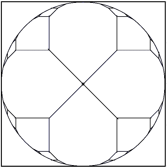
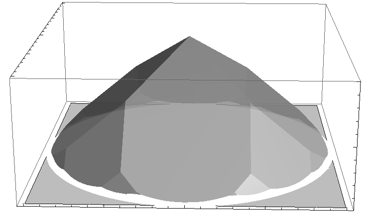
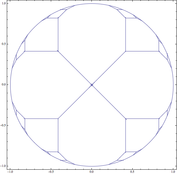
Figure 1. The central picture shows the corner locus of the right picture which is $l_{\Omega}$ (Definition 3.2) for $\Omega=\{x^{2}+y^{2}\leq 1\}$.

Lemma 3.5.

If $\Omega$ is a compact set, then the function $l_{\Omega}$ is an $\Omega$-tropical series.

Proof.

It is enough to prove that $l_{\Omega}$ is zero on $\partial\Omega$ and continuous when we approach $\partial\Omega$. It is clear that $l_{\Omega}=0$ on the points of $\{l^{q}_{\Omega}=0\}\cap\partial\Omega$ for all $q\in\mathcal{A}_{\Omega}$. Consider a point in $\partial\Omega$ where there is no support hyperplane plane with a rational slope. Without loss of generality we may suppose that this point is $0\in\mathbb{R}^{n}$. Pick any support hyperplane $L$ at $0\in\partial\Omega$, let its irrational slope be $\alpha\in\mathbb{R}^{n}$. Consider $r$ big enough (e.g. bigger than the diameter of $\Omega$) and take a ball $B\subset L$ of radius $r$ centered at $0$. Then, for directions $q$ close to $\alpha$, the values of support hyperplane equations $q\cdot z-c_{q}$ at $0$ can be estimated as $|c_{q}|$ which is less than $\max_{z\in B}q\cdot z$.

To prove that $l_{\Omega}$ is an $\Omega$-tropical series it is enough to find a sequence of directions $q_{i}$ close to $\alpha=(\alpha_{1},\dots,\alpha_{n})$ such that $\max_{z\in B}q_{i}\cdot z$ tends to $0$ as $i\to\infty$. We use Dirichlet’s simultaneous approximation theorem and construct a sequence of approximations $(q_{1i,}\dots,q_{ni})\in\mathbb{Z}^{n},r_{i}\in\mathbb{Z}$ such that $|\frac{q_{ki}}{r_{i}}-\alpha_{k}|\leq\frac{1}{r_{i}^{1+1/n}}$. Thus, for each vector $v\in B$ we have $v\cdot(q_{k1}-r_{i}\alpha_{1},\dots,q_{kn}-r_{i}\alpha_{n})\leq\frac{r}{r_{i}^{1/n}}$. Since $v\in B\subset L$ we have $v\cdot\alpha=0$, and by letting $r_{i}\to\infty$ we have the desired property.∎

The function $l_{\Omega}$ is important for all other constructions, this is the pointwise minimal on $\Omega$ non-negative tropical series without the constant term. Therefore for all applications it is important that $l_{\Omega}$ is an $\Omega$-tropical series. In particular $\Omega$ admits non-trivial $\Omega$-tropical series if and only if $l_{\Omega}$ is an $\Omega$-tropical series. It is so if $\Omega$ is a convex compact set, but we failed to find a reasonable criteria (for dimension at least three) for $\Omega$ to imply that $l_{\Omega}$ is zero along $\partial\Omega$. In $\mathbb{R}^{2}$, if $\Omega$ does not contain a line with an irrational slope, then $l_{\Omega}$ is an $\Omega$-tropical series, see [9].

4. Shrinking operators $G_{\bf p}$

Let $f$ be a non-trivial $\Omega$-tropical series. Then $C(f)$ is not empty and divides $\Omega^{\circ}$ into convex connected components. Each connected component of $\Omega^{\circ}\setminus C(f)$ is called a face of $f$ (or, equally, a face of $C(f)$). Let $P=\{{\bf p}_{1},\dots,{\bf p}_{m}\}$ be a finite collection of distinct points in $\Omega^{\circ}$. Let $g$ be an $\Omega$-tropical series.

Definition 4.1.

Denote by $V(\Omega,P,f)$ the set of $\Omega$-tropical series $g$ such that $g|_{\Omega}\geq f$ and each of the points ${\bf p}\in P$ belong to the corner locus of $g$, i.e. $g$ is not smooth at each of ${\bf p}\in P$.

Lemma 4.2.

The set $V(\Omega,P,f)$ is not empty.

Proof.

Indeed, the function

$$f^{\prime}(z)=f(z)+\sum_{{\bf p}\in P}\min(l_{\Omega}(z),l_{\Omega}({\bf p}))$$

belongs to $V(\Omega,P,f)$. ∎

Clearly, if $f\geq g$ then $V(\Omega,P,f)\subset V(\Omega,P,g)$.

Definition 4.3.

For a finite subset $P$ of $\Omega^{\circ}$ and an $\Omega$-tropical series $f$ we define an operator $G_{P}$, given by

$$G_{P}f(z)=\inf\{g(z)|g\in V(\Omega,P,f)\}.$$

If $P$ contains only one point ${\bf p}$ we write $G_{\bf p}$ instead of $G_{\{{\bf p}\}}$.

We call $G_{p}$ shrinking operators because they shrink the domain where $p$ belongs to, as we will see later. In [9] these operators in dimension two were called wave operators, because secretly they correspond to a wave dynamic in a certain sandpile model, see [6, 8]. Here we decided to rebaptize them.

Lemma 4.4.

Let $g$ and $f$ be two tropical series on $\Omega^{\circ}$ such that $g\leq f$ and $P\subset\Omega^{\circ}.$ Then $G_{P}g\leq G_{P}f$.

Proof.

Indeed, $G_{P}f\geq f\geq g$ and $G_{P}f$ is not smooth at $P$. Therefore, $G_{P}g\leq G_{P}f$ by definition of $G_{P}g.$ ∎

Definition 4.5.

We say that a tropical series $f$ on $\Omega$ is presented in the small canonical form if $f$ is written as

$$f(z)=\min_{q\in\mathcal{B}_{f}}(q\cdot z+a_{q})$$ (4.6)

where all $a_{q}$ are taken from the canonical form and $\mathcal{B}_{f}$ consists of monomials $qz+a_{q}$ which are equal to $f$ at at least one point in $\Omega^{\circ}$.

Example 4.7.

The small canonical form for Example 5.3 is $\min(x,y,1-x,1-y,1/3)$.

Figure 2. First row shows how curves given by $G_{p}0_{\Omega}$ depend on the position of the point in the pentagon $\Omega$. The second row shows monomials in their minimal canonical form. Note that the coordinate axes of the second row are actually reversed. Each lattice point on a below picture represents a face where the corresponding monomial is dominating on a top picture, see the bottom-right picture, [9].

Figure 3. On the left: $\Omega$-tropical series $\min(x,y,1-x,1-y,1/3)$ and the corresponding tropical curve. On the right: the result of applying $G_{(\frac{1}{5},\frac{1}{2})}$ to the left picture. The new $\Omega$-tropical series is $\min(2x,x+\frac{2}{15},y,1-x,1-y,\frac{1}{3})$ and the corresponding tropical curve is presented on the right. The fat point is $(\frac{1}{5},\frac{1}{2})$. Note that there appears a new face where $2x$ is the dominating monomial, [9].

In Lemma 5.5 we prove that each individual $G_{\bf p}$ simply contracts one connected component of $\mathbb{R}^{n}\setminus C(f)$ until $C(G_{\bf p}f)$ passes through ${\bf p}$, see Figure 4. In Proposition 6.1 we will prove that $G_{P}$ can be obtained as the limit of repetitive applications $G_{\bf p}$ for ${\bf p}\in P$.

We denote by $0_{\Omega}$ the function $f\equiv 0$ on $\Omega$.

Lemma 4.8.

For ${\bf p}\in\Omega^{\circ}$ we have $G_{{\bf p}}0_{\Omega}(z)=\min(l_{\Omega}(z),l_{\Omega}({\bf p}))$.

Proof.

Indeed, all the coefficients, except $a_{0}$, in the canonical form of $G_{{\bf p}}0_{\Omega}$ can not be less than in $l_{\Omega}$ by Remark 3.3, and if $a_{0}$ were less than $l_{\Omega}({\bf p})$, then the function would be smooth at ${\bf p}$. ∎

Proposition 4.9.

For any $z\in\Omega$ and $P=\{{\bf p}_{1},\dots,{\bf p}_{n}\}$ the following inequality holds

$$G_{P}0_{\Omega}\leq n\cdot l_{\Omega}(z).$$

Proof.

For each point ${\bf p}\in P$ we consider the function $(G_{\bf p}0_{\Omega})(z)=\min(l_{\Omega}(z),l_{\Omega}({\bf p}))$, which is not smooth at ${\bf p}$ and $(G_{\bf p}0_{\Omega})|_{\partial\Omega}=0$. Finally,

$$G_{P}0_{\Omega}\leq\sum_{{\bf p}\in P}G_{\bf p}0_{\Omega}\leq n\cdot l_{\Omega}.$$

∎

Lemma 4.10.

The operator $G_{P}$ maps $\Omega$-tropical series to $\Omega$-tropical series.

Proof.

Let $f$ be an $\Omega$-tropical series, $g\in V(\Omega,P,f)$, $z_{0}\in\Omega^{\circ}$ and $K\subset\Omega^{\circ}$ be a compact set such that $z_{0}\in K^{\circ}$. Denote by $\text{C}>0$ the maximum of $g$ on $K$. Consider the set $\mathcal{M}$ of all $p\in\mathbb{Z}^{n}$ for which there exist $d\in\mathbb{R},z_{0}\in K$ such that $0\leq(p\cdot z_{0}+d)|_{\Omega^{\circ}},p\cdot z_{0}+d\leq\text{C}.$ The set $\mathcal{M}$ is finite by Lemma 2.4. Therefore, the restriction of any tropical series $g\in V(\Omega,P,f)$ to $K$ can be expressed as a tropical polynomial $\min_{p\in\mathcal{M}}(p\cdot z+a_{p}(g))$. In particular, if we denote by $a_{p}$ the infimum of $a_{p}(g)$ for all $g\in V(\Omega,P,f)$ then

$$G_{P}f|_{K}=\min_{p\in\mathcal{M}}(p\cdot z+a_{p}),$$

so $G_{P}f$ is a tropical series.

It follows from Proposition 4.9, that $G_{P}f\leq f+n\cdot l_{\Omega}$. Then, $l_{\Omega}|_{\partial\Omega}=0$ by Lemma 3.5. Therefore $G_{P}f|_{\partial\Omega}=0$ and, thus, Lemma 2.7 concludes the proof that $G_{P}f$ is an $\Omega$-tropical series. ∎

Remark 4.11.

Let $f=G_{P}0_{\Omega}$ and $\varepsilon$ is such that $f({\bf p}_{i})>\varepsilon$ for each ${\bf p}_{i}\in P$. Then $G_{P}0_{\Omega}=G_{P}\min(f(z),\varepsilon)$.

Indeed, $\min(f(z),\varepsilon)\geq 0_{\Omega}$ therefore $G_{P}\min(f(z),\varepsilon)\geq G_{P}0_{\Omega}$. Then, $G_{P}0_{\Omega}\geq\min(f(z),\varepsilon)$ and not smooth at each of ${\bf p}_{i}$, therefore $G_{P}0_{\Omega}\leq G_{P}\min(f(z),\varepsilon)$.

5. Flow version of operators $G_{\bf p}$

Note that an $\Omega$-tropical series $f:\Omega\to\mathbb{R}$ may have different presentations as the minimum of linear functions. For example, if $\Omega$ is the square $[0,1]\times[0,1]\subset\mathbb{R}^{2}$, then $\min(x,1-x,y,1-y,1/3)$ equals at every point of $\Omega$ to $\min(x,1-x,y,1-y,1/3,2x,5-2x)$.

Definition 5.1 (cf. [11], Lemma 5.3).

To resolve this ambiguity, we suppose that, in $\Omega^{\circ}$, a tropical series $f$ is always (if the opposite is not stated explicitly) given by

$$f(z)=\min\limits_{q\in\mathcal{A}}(q\cdot z+c_{q})$$ (5.2)

with $\mathcal{A}=\mathcal{A}_{\Omega}$ (Definition 3.1) and with as minimal as possible coefficients $c_{q}$. We call this presentation the canonical form of a tropical series. For each $\Omega$-tropical series there exists a unique canonical form.

Example 5.3.

The canonical form of $\min(x,1-x,y,1-y,1/3)$ on $\Omega=[0,1]\times[0,1]$ is $f(x,y)$ as in (5.2) with $\mathcal{A}=\mathbb{Z}^{2}$, $a_{00}=1/3$ and $a_{ij}=-\min_{(x,y)\in\Omega}(ix+jy)$ for $(i,j)\in\mathbb{Z}^{2}\setminus\{(0,0)\}$.

Proof.

It is easy to check that $f(x,y)=\min(x,1-x,y,1-y,1/3)$ on $\Omega$. All the coefficients $a_{ij},(i,j)\neq(0,0)$ are chosen as minimal with the condition that $ix+jy+a_{ij}$ is non-negative on $\Omega$. Finally, in the canonical form of $\min(x,1-x,y,1-y,1/3)$ the coefficient $a_{00}$ can not be less than $1/3$. ∎

We define the following operator $\mathrm{Add}_{p}^{c}$ on tropical series, which adds a constant $c$ to the coefficient $a_{p}$ in tropical monomial $p\cdot z$, leaving other coefficients unchanged.

Definition 5.4.

For an $\Omega$-tropical series $f$ in the canonical form (see (5.2), Definition 5.1) and $c\geq 0,q\in\mathbb{Z}^{n}$ we denote by $\mathrm{Add}_{q}^{c}f$ the $\Omega$-tropical series

$$(\mathrm{Add}_{q}^{c}f)(z)=\min\left(a_{q}+c+q\cdot z,\min\limits_{\begin{subarray}{c}{p\in\mathbb{Z}^{n}}\\ {p\neq q}\end{subarray}}(a_{p}+p\cdot z)\right).$$

Figure 4. Illustration for Remark 5.9. The operator $G_{\bf p}$ shrinks the connected component $\Phi$ (face) of $\Omega\setminus C(f)$ where ${\bf p}$ belongs to. Firstly, $t=0$, then $t=0.5$, and finally $t=1$ in $\mathrm{Add}_{q}^{ct}f$. Note that combinatorics of the curve can change when $t$ goes from $0$ to $1$. Similar pictures can be found in [19], see Figure 2.

Lemma 5.5.

Let $f=\min_{q\in\mathcal{A}_{\Omega}}(q\cdot z+a_{q})$ be an $\Omega$-tropical series in the canonical form, suppose that ${\bf p}\in\Omega^{\circ}\setminus C(f)$. Suppose that $f$ is equal to $q_{0}\cdot z+a_{q_{0}}$ near ${\bf p}$. Consider the function

$$g(z)=\min_{q\in\mathbb{Z}^{n},q\neq q_{0}}(q\cdot z+a_{q}).$$ (5.6)

Then, $G_{\bf p}f=\mathrm{Add}_{q_{0}}^{c}f$ with $c=g({\bf p})-q_{0}\cdot{\bf p}$.

Proof.

$G_{\bf p}(f)$ is at most $\min\left(g,q_{0}\cdot z+(g({\bf p})-q_{0}\cdot{\bf p})\right)$ by definition. Therefore $f$ and $G_{\bf p}f$ differ only at one monomial. Also, direct calculation shows that $\min(g,q_{0}\cdot z+c)$ is smooth at ${\bf p}$ as long as $c<g({\bf p})-q_{0}\cdot{\bf p}$, which finishes the proof. ∎

Definition 5.7.

A connected component of $\Omega\setminus C(f)$ is called a face.

Each face is a domain of linearity of $f$, thus to each face $\Phi$ there correspond a monomial $qz+a_{q}$ if $f$ and $f(z)|_{\Phi}=qz+a_{q}$.

Corollary 5.8.

In the notation of Definition 3.2, for a point ${\bf p}\in\Omega^{\circ}$, for each $z\in\Omega$ we have

$$(G_{\bf p}0_{\Omega})(z)=\min\{l_{\Omega}(z),l_{\Omega}({\bf p})\}.$$

Remark 5.9.

Suppose that $G_{\bf p}f=\mathrm{Add}_{q}^{c}f$. We can include the operator $\mathrm{Add}_{q}^{c}$ into a continuous family (flow) of operators

$$f\to\mathrm{Add}_{q}^{ct}f,\text{\ where $t\in[0,1]$}.$$

This allows us to observe the tropical curve during the application of $\mathrm{Add}_{q}^{c}$, in other words, we look at the family of curves defined by tropical series $\mathrm{Add}_{q}^{ct}f$ for $t\in[0,1]$, this is a flow on the space of tropical series. See Figure 4.

Note that this defines a continuous dynamic since the curve changes by a continuous shrinking a face, explaining the name of operators.

6. Dynamic generated by $G_{\bf p}$ for ${\bf p}\in P$.

Recall that $P=\{{\bf p}_{i}\}_{i=1}^{n},P\subset\Omega^{\circ}$. Let $\{{\bf p}_{1}^{\prime},{\bf p}_{2}^{\prime},\dots\}$ be an infinite sequence of points in $P$ where each point ${\bf p}_{i},i=1,\dots,n$ appears infinite number of times. Let $f$ be any $\Omega$-tropical series. Consider a sequence of $\Omega$-tropical series $\{f_{m}\}_{m=1}^{\infty}$ defined recursively as

$$f_{1}=f,f_{m+1}=G_{{\bf p}_{m}^{\prime}}f_{m}.$$

Proposition 6.1.

The sequence $\{f_{m}\}_{m=1}^{\infty}$ uniformly converges to $G_{P}f$.

Proof.

First of all, $G_{P}f$ has an upper bound $f+nl_{\Omega}$ by arguments as in Proposition 4.9. Applying Lemma 4.4, induction on $m$ and the obvious fact that $G_{{\bf p}_{m}}G_{P}f=G_{P}f$ we have that $f_{m}\leq G_{P}f$ for all $m.$ It follows from Lemmata 2.4, 5.5 that $G_{{\bf p}_{m}^{\prime}},m=1,\dots$ change only a certain fixed finite subset of monomials in $f_{m}$ (which can in principle contribute to a tropical series in a neighborhood of points in $P$). This implies the uniform convergence: since the family $\{f_{m}\}_{m=1}^{\infty}$ is pointwise monotone and bounded, it converges to some $\Omega$-tropical series $\tilde{f}\leq G_{P}f$. Indeed, to find the canonical form of $\tilde{f}$ we can take the limits (as $m\to\infty$) of the coefficients for $f_{m}$ in their canonical forms (5.2).

It is clear that $\tilde{f}$ is not smooth at all the points $P$. Therefore, by definition of $G_{P}$ we have $\tilde{f}\geq G_{P}f$, which finishes the proof. ∎

Remark 6.2.

Note that in the case when $\Omega$ is a lattice polytope and the points $P$ are lattice points, all the increments $c$ of the coefficients in $G_{\bf p}=\mathrm{Add}_{q}^{c}$ are integers, and therefore the sequence $\{f_{m}\}$ always stabilizes after a finite number of steps.

Lemma 6.3.

Let $\varepsilon>0,\mathcal{B}\subset\mathbb{Z}^{n}$ be a finite set, and $f,g$ be two tropical series in $\Omega^{\circ}$ written as

$$f(z)=\min_{q\in\mathcal{B}}(q\cdot z+a_{q}),g(z)=\min_{q\in\mathcal{B}}(q\cdot z+a_{q}+\delta_{q}).$$

If $|\delta_{q}|<\varepsilon$ for each $q\in\mathcal{B}$, then $C(f)$ is $2\varepsilon$-close to $C(g)$. If, moreover, all $\delta_{q}$ are of the same sign, then $C(f)$ is $\varepsilon$-close to $C(g)$.

Proof.

Let $p\in C(f)$, $q_{1}z+a_{q_{1}},q_{2}z+a_{q_{2}}$ be two monomials of $f$, which are minimal at $p$. Suppose that $B_{2\varepsilon}(p)\cap C(g)=\varnothing$. Therefore $g|_{B_{2\varepsilon}(p)}=q_{3}z+a_{q_{3}}+\delta_{q_{3}}$. Then, $q_{3}\neq q_{1}$ without loss of generality. We rewrite all this information as $q_{1}p+a_{q_{1}}=q_{2}p+a_{q_{2}}\leq q_{3}p+a_{q_{3}}$ and $q_{3}z+a_{q_{3}}+\delta_{q_{3}}<q_{1}z+a_{q_{1}}+\delta_{q_{1}}$ on $B_{2\varepsilon}(p)$.

Therefore $q_{3}z+a_{q_{3}}+\delta_{q_{3}}-(q_{1}z+a_{q_{1}}+\delta_{q_{1}})\geq\delta_{q_{3}}-\delta_{q_{1}}$ at $z=p$ and strictly negative on $B_{2\varepsilon}(p)$. Note that $|\delta_{q_{3}}-\delta_{q_{1}}|<2\varepsilon$ (and $|\delta_{q_{3}}-\delta_{q_{1}}|\leq\varepsilon$ if $\delta_{q_{3}},\delta_{q_{1}}$ are of the same sign) but the maximum of $(q_{3}-q_{1})z$ on $B_{r}$ is at least $r\cdot|q_{1}-q_{3}|\geq r$ which finishes the proof in both cases.

∎

Corollary 6.4.

Using Lemma 6.3 we may include the dynamic $f=f_{1}\to f_{2}\to f_{3}\to\dots\to G_{P}f$ into a continuous dynamic with time $t\in[0,1]$. Indeed, let us rescale the time and perform $f_{1}\to f_{2}$ on $[0,1/2]$, then $f_{2}\to f_{3}$ on $[1/2,3/4]$, etc. By Proposition 6.1 and Remark 5.9 this extends continuously near $t=1$.

Remark 6.5.

Let ${\bf p^{\prime}_{i}}\in P$ for $i=1,\dots,m$ (we allow repetitions). Note that if $G_{{\bf p^{\prime}}_{m}}\dots G_{{\bf p^{\prime}}_{1}}f$ is close to the limit $G_{P}f$, then by Lemma 6.3 we see that the corresponding tropical curves are also close to each other.

Definition 6.6.

For two $\Omega$-tropical series $f=\inf(q\cdot z+a_{q}),q\in\mathcal{B}$ and $g=\inf(q\cdot z+b_{q}),q\in\mathcal{B}$ we define $\rho(f,g)=\sup_{\mathcal{B}}(|a_{q}-b_{q}|)$.

Lemma 6.7.

If $f,g$ are two $\Omega$-tropical series and ${\bf p}\in\Omega^{\circ}$, then $\rho(G_{\bf p}f,G_{\bf p}g)\leq\rho(f,g)$.

Proof.

For each $z\in\Omega$ we have $|f(z)-g(z)|\leq\rho(f,g)$. Therefore, if ${\bf p}$ belong to the face where $q\cdot z+a_{q}=f(z)$ and $q\cdot z+b_{q}=g(z)$, then it follows from Lemma 5.5 that the coefficients $a_{q},b_{q}$ in monomial $q\cdot z$ in $G_{\bf p}f,G_{\bf p}g$ differ by at most $\rho(f,g)$.

Let ${\bf p}$ belong to different faces in $C(f),C(g)$, i.e. $q\cdot z+a_{q}=f(z),q^{\prime}\cdot z+b_{q^{\prime}}=g(z)$ near ${\bf p}$. Without loss of generality we may suppose that $q^{\prime}=0\in\mathbb{Z}^{n}$ and ${\bf p}=0\in\mathbb{R}^{n}$. Therefore, $a_{q}\leq a_{0},b_{q}\geq b_{0},a_{0}\leq b_{0}+\rho(f,g)$. Finally, $G_{\bf p}f$ increases $a_{q}$, clearly new $a_{q}$ is at most $a_{0}\leq b_{0}+\rho(f,g)\leq b_{q}+\rho(f,g)$. Other inequalities for the coefficients can be obtained similarly. ∎

7. Mild singularities

Recall that for a tropical hypersurface $C(f)$ the connected components (we already called them faces) of $\mathbb{R}^{n}\setminus C(f)$ correspond to monomials in $f$ (this monomial is the minimal one on that connected component). Then, in general, faces of maximal dimension (i.e. $n-1$) in $C(f)$ correspond to pairs of monomials of $f$, which are equal along this face. Faces of $C(f)$ of dimension $n-2$ correspond to triples of monomials equal along such a face, etc. The general statement is as follows. Let us pick a tropical series

$$f(z)=\min_{q\in\mathcal{B}}(q\cdot z+a_{q})$$

Consider the extended Newton polytope $\tilde{N}(f)$, i.e. the convex hull of the set

$$N(f)=\{(q,r)\in\mathbb{Z}^{n}\times\mathbb{R}|q\in\mathcal{B},r\geq a_{p}\}.$$

The projection of faces of $\tilde{N}(f)$ along the last coordinates defines a subdivision of the convex hull $\tilde{\mathcal{B}}$ of $\mathcal{B}$. This subdivision is dual to the the combinatorial structure of $C(f)$. To each point $z\in C(f)$ there corresponds a set $\mathcal{B}_{z}$ of monomials of $f$, which are minimal at $z$. This convex hull $\tilde{\mathcal{B}}_{z}$ of $\mathcal{B}_{z}$ is a face of the aforementioned subdisivion. And vice versa, to each face $\tilde{\mathcal{B}}_{V}$ of dimension $k$ of this subdivision of $\tilde{B}$ there corresponds a subset $V$ of points $z$ of $C(f)$ such that $\tilde{\mathcal{B}}_{V}=\tilde{\mathcal{B}}_{z}$ for each $z\in V$, and this subset $V$ is a face of $C(f)$.

Definition 7.1.

We say that $f$ (or $C(f)$) has only mild singularities if for each $z\in C(f)$ the lattice polytope $\tilde{\mathcal{B}}_{z}$ contains no lattice points except its vertices.

Remark 7.2.

Another, equivalent definition is as follows: $f$ has only mild singularities if for each $q\in\tilde{B}$ there exists an open subset of $\Omega$ where the monomial of $f$, corresponding to $q$ is the minimal monomial.

This terminology comes from the case of planar tropical curves. In $\mathbb{Z}^{2}$, the lattice polygons with no lattice points except vertices are primitive vectors in $\mathbb{Z}^{2}$ (this corresponds to edges of the tropical curve of multiplicity one), triangles of area $1/2$ (this corresponds to smooth vertices of the tropical curve) and parallelograms of area one (this corresponds to nodal points of the tropical curve).

Lemma 7.3.

Let $f$ be an $\Omega$-tropical hypersurface with only mild singularities. Consider any face $\Phi$ of it, of any dimension (e.g. a vertex of this gypersurface). There exists no $q\in\mathbb{Z}^{n},a_{q}\in\mathbb{R}$ such that $\min(f(z),qz+a_{q})$ coincides with $f$ outside of a small neighborhood of $\Phi$.

Proof.

If such $q$ could exists, it would mean that $q$ belongs to a convex hull of $\tilde{\mathcal{B}}_{z},z\in\Phi$ and does not coincide with any of its vertices, which is a contradiction. Indeed, if $q$ can be separated from the convex set $\tilde{\mathcal{B}}_{z}$ by a hyperplane, then moving from $z$ in the direction orthogonal to this hyperplane, we would get that $qz+a_{q}$ decreases faster then all monomials in $f(z)$, and therefore it is not true that $\min(f(z),qz+a_{q})$ coincides with $f$ outside of a small neighborhood of $\Phi$. ∎

Definition 7.4.

Let $\Delta\subset\mathbb{R}^{n}$ be a finite intersection of half-spaces (at least one) with normals in $\mathbb{Z}^{n}$. We call $\Delta$ a $\mathbb{Q}$-polygon if it has non-empty interior.

Definition 7.5.

A face $F$ (of any codimension) of a $\mathbb{Q}$-polytope $\Delta$ is called mild if the convex hull of the origin and the set of primitive lattice vectors orthogonal to all hyperfaces of $\Delta$ containing $F$ contains no lattice points except vertices.

Note that any hyperface is automatically mild, because of the definition of the primitive vector of given direction. Then, in $\mathbb{Z}^{2}$ a vertex of a polygon is mild if an only if the primitive vectors in the directions of its edges constitute a basis of $\mathbb{Z}^{2}$.

Lemma 7.6.

Let $\Delta\subset\mathbb{R}^{n}$ be a $\mathbb{Q}$-polytope whose all faces are mild. Let $f$ be a $\Delta$-tropical series such that $C(f)$ has only mild singularities. Let $p\in\Delta\setminus C(f)$. Let $G_{p}f=\mathrm{Add}_{q}^{c}f$. Then, for each $t\in[0,1)$ the $\Delta$-tropical series $\mathrm{Add}_{q}^{ct}f$ has only mild singularities.

Proof.

Consider the changes of the extended Newton polytope $\tilde{N}(f)$ of $f$ while applying $\mathrm{Add}_{q}^{ct}$ to $f$. The coefficient of $q$ grows so the corresponding to $q$ vertex of $\tilde{N}(f)$ goes up and there can be some changes of $\tilde{N}(f)$, but the set of vertices is preserved. Therefore no lattice point can be found inside the sets $\tilde{B}_{V}$ except their vertices, therefore $\mathrm{Add}_{q}^{ct}f$ has only mild singularities. Note that the point $(q,a_{q}+tc)$ may fail to be a vertex of $\tilde{N}(f)$ only if its corresponding face in $C(f)$ contracts, and this can happen only at $t=1$. ∎

Corollary 7.7.

The only case when $G_{p}f$ not not have only mild singularities is when the monomial $q$ does not contribute to $G_{p}f$ in the sense that the set of points $z$ where $qz+a_{q}$ is strictly less then all the other monomials in $G_{p}f$ is empty.

8. Approximations of a compact convex domain by $\mathbb{Q}$-polygons

Definition 8.1.

Let ${\bf p}_{1},\dots\bf p_{n}\in\Omega^{\circ}$ be different points, $P=\{{\bf p}_{1},\dots,{\bf p}_{n}\}$. We denote by $f_{\Omega,P}$ the pointwise minimum among all $\Omega$-tropical series non-smooth at all the points ${\bf p}_{1},\dots,{\bf p}_{n}$.

Lemma 8.2.

If $\Omega$ is bounded, then for any $\varepsilon>0$ the set $\Omega_{\varepsilon}=\{x\in\Omega|f_{\Omega,P}\geq\varepsilon\}$ is a $\mathbb{Q}$-polygon and $f_{\Omega,P}|_{\Omega_{\varepsilon}}$ is a tropical polynomial.

Proof.

Note that $G_{P}0_{\Omega}=f_{\Omega,P}(x)$ by the definition of the latter, so it follows from Lemma 4.10 that $f_{\Omega,P}$ is continuous and vanishes at $\partial\Omega$. Since $\Omega$ is bounded, the set $f_{\Omega,P}=\varepsilon$ is a curve disjoint from $\partial\Omega.$ We claim that the intersection of $\Omega_{\varepsilon}$ with $C(f_{\Omega,P})$ is a tropical hypersurface with a finite number of vertices. Suppose the contrary. Then a sequence of vertices of this hypersurface converges to a point $z\in\Omega^{\circ}.$ Thus, there is no neighborhood of $z$ where the series $f_{\Omega,P}$ can be represented by a tropical polynomial, which is a contradiction with Definition 1.2. The finiteness of the number of vertices implies that there is only a finite number of monomials participating in the restriction of $f_{\Omega,P}$ to the domain $\Omega_{\varepsilon},$ therefore the restriction is a tropical polynomial. ∎

Lemma 8.3.

In the above hypothesis, we extend $f_{\Omega_{\varepsilon},P}$ to $\Omega$ using the presentation of $f_{\Omega_{\varepsilon},P}$ in the small canonical form (Definition 4.5). In the hypothesis of the previous lemma, if $f_{\Omega,P}({\bf p})\geq\varepsilon$ for each ${\bf p}\in P$, then we have $f_{\Omega,P}=f_{\Omega_{\varepsilon},P}+\varepsilon$ on $\Omega_{\varepsilon}$. Also $f_{\Omega_{\varepsilon},P}+\varepsilon\geq f_{\Omega,P}$ on $\Omega$.

Proof.

On $\Omega_{\varepsilon}$ we have that $f_{\Omega,P}-\varepsilon\geq f_{\Omega_{\varepsilon},P}$ by the definition of the latter. Then, two functions $f_{\Omega_{\varepsilon},P}+\varepsilon,f_{\Omega,P}$ are equal on $\partial\Omega_{\varepsilon}$ and by the previous line the quasi-degree of $f_{\Omega_{\varepsilon},P}$ is at most the quasi-degree of $(f_{\Omega,P}-\varepsilon)|_{\Omega_{\varepsilon}}$. Hence $f_{\Omega,P}$ can not decrease slowly than $f_{\Omega_{\varepsilon},P}$ when we move from $\partial\Omega_{\varepsilon}$ towards $\partial\Omega$. Therefore $f_{\Omega_{\varepsilon},P}+\varepsilon\geq f_{\Omega,P}$ on $\Omega\setminus\Omega_{\varepsilon}$. Since $f_{\Omega_{\varepsilon},P}+\varepsilon\geq 0$ on $\Omega$ we obtain the estimate $f_{\Omega_{\varepsilon},P}+\varepsilon\geq f_{\Omega,P}$ on $\Omega$ which concludes the proof. ∎

9. The main theorem

Let $\Omega\subset\mathbb{R}^{n}$ be a compact convex domain and $P=\{p_{1},\dots,p_{m}\}\in\Omega^{\circ}$ a set of points. As we know, $G_{P}0_{\Omega}$ can be obtained as the limit of a continuous family of shrinking operators (Proposition 6.1, Lemma 5.5, Remark 5.9),

$$G_{P}0_{\Omega}=(\prod\limits_{i=1}^{\infty}\mathrm{Add}_{w_{i}}^{t_{i}})0_{\Omega},$$

where $w_{i}\in P,t_{i}\in\mathbb{R}_{\geq 0}$.

Theorem 1.

For each $\varepsilon>0$ there exists $\delta>0$ and a $\mathbb{Q}$-polytope $Q\subset\Omega$ and a $Q$-tropical series $g(z)<\delta,\forall z\in Q$, such that $C(g)$ has only mild singularities. Moreover, for $N$ big enough a continuous operator

$$F=\prod\limits_{i=1}^{N}\mathrm{Add}_{w_{i}}^{t_{i}-\delta},$$

a composition of continuous operators $\mathrm{Add}$ (see Remark 5.9), produces $Q$-tropical series $F(g):Q\to\mathbb{R}_{\geq 0}$ which is $\varepsilon$-close to $G_{P}0_{\Omega}$ on $\Omega$ and during computation of $F(g)$ all appearing $Q$-tropical hypersurfaces have only mild singularities.

We can summarise this theorem in the following diagram, where the first row is on $\Omega$ and the second row is on $Q$:

In other words, we need to get from $0_{\Omega}$ to $G_{P}0_{\Omega}$ but we want to avoid too singular tropical hypersurfaces. Thus we slightly change the domain (we consider $Q\subset\Omega$ instead of $\Omega$), then change $0_{\Omega}$ to a $Q$-tropical series $g$, which is close to $0$, then approximate $G_{P}$ by a family of shrinking operators avoiding too singular hypersurfaces. And, using our machinery, we prove that the result of these approximations can be arbitrary close to $G_{P}0_{\Omega}$.

Proof.

Pick an $\varepsilon>0$. As in Lemma 8.2 choose small $\varepsilon^{\prime}$ and define $Q^{\prime}=\{z\in\Omega|G_{P}0_{\Omega}(z)\geq\varepsilon^{\prime}\}$. Note that $g_{1}=G_{P}0_{\Omega}-\varepsilon^{\prime}$ is a $Q^{\prime}$-tropical series on $Q^{\prime}$ and has a small canonical form (Definition 4.5) on $Q^{\prime}$ with a finite $\mathcal{B}^{\prime}$, i.e.

$$g_{1}(z)=\min_{q\in\mathcal{B}^{\prime}}(q\cdot z+a_{q}).$$

As in Remark 4.11, we see that $\varepsilon^{\prime}+G_{P}g_{1}$ is equal to $G_{P}0_{\Omega}$ on $Q^{\prime}$. Choose $\varepsilon^{\prime\prime}$ very small and define $g_{1}(z)=\min(g_{1}(z),\varepsilon^{\prime\prime})$ on $Q^{\prime}$.

Let $\mathcal{B}$ be the intersection of the convex hull of $\mathcal{B}^{\prime}$ with $\mathbb{Z}^{n}$. Write $g_{1}(z)$ on $Q^{\prime}$ in the canonical form, and then slightly diminish coefficients corresponding to monomials in $\mathcal{B}\setminus B^{\prime}$, the obtained function is denoted by $g$. Define $Q=\{z|g(z)=0\}$. Thus, $Q$-tropical series $g$ is close to $g_{2}$ on $Q$. Also, $C(g)$ has only mild singularities by Remark 7.2.

It follows from our construction that $G_{P}g=g$ near the boundary of $Q$ (see Remark 4.11), therefore $G_{P}g$ is close to $G_{P}0_{\Omega}$.

Next, choose $N$ big enough that $\prod\limits_{i=1}^{N}\mathrm{Add}_{w_{i}}^{t_{i}}g$ is close to $G_{P}g$ (see Proposition 6.1). Then diminish $t_{i}$ by $\delta$, and by Lemma 7.6 we obtain that the flow $F(g)=\prod\limits_{i=1}^{N}\mathrm{Add}_{w_{i}}^{t_{i}-\delta}g$ contains $Q$-tropical hypersurfaces with mild singularities only, and if $\delta$ is small enough then $F(g)$ is close to $G_{P}g$ which finishes the proof. ∎

Nikita Kalinin,

References

• [1] E. Abakumov and E. Doubtsov, Approximation by proper holomorphic maps and tropical power series, Constructive Approximation, 1–18, URL http://dx.doi.org/10.1007/s00365-017-9375-5.
• [2] E. Brugallé, Some aspects of tropical geometry, Eur. Math. Soc. Newsl., 23–28.
• [3] E. Brugallé, I. Itenberg, G. Mikhalkin and K. Shaw, Brief introduction to tropical geometry, in Proceedings of the Gökova Geometry-Topology Conference 2014, Gökova Geometry/Topology Conference (GGT), Gökova, 2015, 1–75.
• [4] S. Caracciolo, G. Paoletti and A. Sportiello, Conservation laws for strings in the abelian sandpile model, EPL (Europhysics Letters), 90 (2010), 60003.
• [5] R. G. Halburd and N. J. Southall, Tropical Nevanlinna theory and ultradiscrete equations, Int. Math. Res. Not. IMRN, 887–911, URL http://dx.doi.org/10.1093/imrn/rnn150.
• [6] N. Kalinin and M. Shkolnikov, Tropical curves in sandpiles, Comptes Rendus Mathematique, 354 (2016), 125–130.
• [7] N. Kalinin, A. Guzmán-Sáenz, Y. Prieto, M. Shkolnikov, V. Kalinina and E. Lupercio, Self-organized criticality and pattern emergence through the lens of tropical geometry, Proceedings of the National Academy of Sciences, 115 (2018), E8135–E8142.
• [8] N. Kalinin and M. Shkolnikov, Tropical curves in sandpile models, arXiv:1502.06284.
• [9] N. Kalinin and M. Shkolnikov, Introduction to tropical series and wave dynamic on them, Discrete & Continuous Dynamical Systems-A, 38 (2018), 2843–2865.
• [10] C. O. Kiselman, Croissance des fonctions plurisousharmoniques en dimension infinie, Ann. Inst. Fourier (Grenoble), 34 (1984), 155–183, URL http://www.numdam.org/item?id=AIF_1984__34_1_155_0.
• [11] C. O. Kiselman, Questions inspired by Mikael Passare’s mathematics, Afrika Matematika, 25 (2014), 271–288.
• [12] R. Korhonen, I. Laine and K. Tohge, Tropical value distribution theory and ultra-discrete equations, World Scientific, 2015.
• [13] S. Lahaye, J. Komenda and J.-L. Boimond, Compositions of (max,+) automata, Discrete Event Dynamic Systems, 25 (2015), 323–344.
• [14] I. Laine and K. Tohge, Tropical Nevanlinna theory and second main theorem, Proc. Lond. Math. Soc. (3), 102 (2011), 883–922, URL http://dx.doi.org/10.1112/plms/pdq049.
• [15] S. Lombardy and J. Sakarovitch, Sequential?, Theoretical Computer Science, 356 (2006), 224–244.
• [16] G. Mikhalkin, Tropical geometry and its applications, in International Congress of Mathematicians. Vol. II, Eur. Math. Soc., Zürich, 2006, 827–852.
• [17] G. Mikhalkin and I. Zharkov, Tropical curves, their Jacobians and theta functions, in Curves and abelian varieties, vol. 465 of Contemp. Math., Amer. Math. Soc., Providence, RI, 2008, 203–230, URL http://dx.doi.org/10.1090/conm/465/09104.
• [18] K. Tohge, The order and type formulas for tropical entire functions—another flexibility of complex analysis, on Complex Analysis and its Applications to Differential and Functional Equations, 113–164.
• [19] C. Vafa, Supersymmetric partition functions and a string theory in 4 dimensions, arXiv preprint arXiv:1209.2425.