On the Existence of Fast Modes in Compressible Magnetohydrodynamic Turbulence

Abstract

We study the existence and property of Fast magnetosonic modes in 3D compressible MHD turbulence by carrying out a number of simulations with compressible and incompressible driving conditions. We use two approaches to determine the presence of Fast modes: mode decomposition based on spatial variations only and spatio-temporal 4D-FFT analysis of all fluctuations. The latter method enables us to quantify fluctuations that satisfy the dispersion relation of Fast modes with finite frequency. Overall, we find that the fraction of Fast modes identified via spatio-temporal 4D FFT approach in total fluctuation power is either tiny with nearly incompressible driving or $\sim 2\%$ with highly compressible driving. We discuss the implications of our results for understanding the compressible fluctuations in space and astrophysics plasmas.

1 Introduction

Magnetized plasma systems, such as magnetic fusion experiments (e.g., Diamond et al., 2005), solar wind (e.g., Matthaeus & Goldstein, 1982), interstellar medium (e.g., Armstrong et al., 1995), and intracluster medium (e.g., Hitomi Collaboration et al., 2018), are often turbulent. Magnetohydrodynamics (MHD) is generally employed to describe turbulence in such systems. Understanding the nature of compressible fluctuations is also critical in describing the relationship between the weak and strong turbulence limits (e.g., Chandran, 2005; Galtier, 2009; Meyrand et al., 2016; Galtier, 2018), because the cascade process, anisotropy, and energy spectrum are likely all modified by compressible effects.

The eigenmodes in a compressible MHD system are different from those in the incompressible limit. We choose to focus on Fast magnetosonic modes or Fast modes in this study. Fast modes are often included in global solar wind models, critical in preferential ion heating at kinetic scales through turbulent cascade (e.g., Cranmer & Ballegooijen, 2012). They may also play an important role in interpreting the recent Voyager 1 observations (Zank et al., 2017, 2019; Burlaga et al., 2018; Zhao et al., 2020). Fast modes have also been used in accelerating particles in solar flares (e.g., Miller et al., 1996), cosmic rays (e.g., Schlickeiser, 2002), and in scattering cosmic rays in the interstellar medium (e.g., Yan & Lazarian, 2002). Furthermore, it is postulated that Fast mode turbulence is effective in producing stochastic particle acceleration in various high-energy astrophysical systems as well (e.g., Dermer et al., 1996; Li & Miller, 1997; Demidem et al., 2020).

Earlier studies have examined the fraction of compressible modes in MHD turbulence and their cascade properties. The primary method is to use only the spatial variations of various variables and decompose them into three eigenmodes – Fast, Slow and Alfvén modes (see e.g. Marsch 1986; Cho & Lazarian 2003; Zhang et al. 2015; Yang et al. 2018). The effects of turbulence driving conditions have been examined in Makwana & Yan (2020), and they found that the Fourier power in Fast modes could be up to $\sim$30% of the total turbulent power if the turbulence driving is highly compressible, and the power in slow modes is even more significant.

Another interesting approach in identifying Fast modes in a turbulence simulation was discussed in Svidzinski et al. (2009). They demonstrated that a spatio-temporal analysis method can be used to decompose the fluctuations (say magnetic fields) using Fast Fourier Transform (FFT) in both spatial and temporal domains, if a large number of data volumes at different time slices are stored to resolve both low and high frequencies (we will refer this approach as 4D FFT). Similar approaches have also been applied to MHD turbulence simulations (e.g., Dmitruk & Matthaeus, 2007, 2009; Clark di Leoni et al., 2015; Meyrand et al., 2016; Andrés et al., 2017; Lugones et al., 2019; Yang et al., 2019; Brodiano et al., 2021), as well as in hybrid kinetic simulations (Markovskii & Vasquez, 2020). Dmitruk & Matthaeus (2007, 2009) examined spatio-temporal turbulence signals in the incompressible regime. The existence of compressible modes (Fast and Slow waves) that satisfy dispersion relations in the frequency-wavenumber ($\omega$ vs ${\bf k}$) space (e.g., Andrés et al., 2017; Yang et al., 2019) has also been demonstrated. Following these earlier studies, we build similar 4D FFT routines to analyze MHD turbulence. In particular, the recent paper by Brodiano et al. (2021) is most similar to the study presented here. They studied the effects of how the compressible vs. incompressible driving affects the presence of waves in turbulence. They concluded that the system is mainly dominated by the nonlinear fluctuations (i.e., not waves).

In this paper, we aim at addressing the detailed properties of Fast modes in compressible MHD turbulence, particularly the existence of finite frequency waves and how they vary under different turbulence driving conditions. In §2 we describe our simulation set-ups and various runs we performed. In §3 we present our analysis and results of numerical simulations. Conclusions and implications of our results are given in §4.

2 Model Description

2.1 Numerical Schemes

To address the existence and properties of Fast modes in compressible MHD turbulence, we solve the time-dependent ideal MHD equations numerically in a three-dimensional Cartesian coordinate system ($x,y,z$) using the code ATHENA++ (Stone et al., 2020). We introduce ${\bf f_{\rm v}}$ and ${\bf f_{\rm B}}$ terms in the momentum and induction equations as turbulence driving forces on velocity and magnetic fields, respectively. Both ${\bf f_{\rm v}}$ and ${\bf f_{\rm B}}$ take the form of ${\bf A}\sin({\bf k}\cdot{\bf x}+\phi)$ across the computational domain with wave numbers ${\bf k}$ that satisfy periodical boundary, and randomly selected phases $\phi$, and amplitudes ${\bf A_{v}}$, ${\bf A_{B}}$ for velocity and magnetic fields, respectively. The amplitude is decomposed into components parallel and perpendicular to the background magnetic field ${\bf B}_{0}$ as ${\bf A_{\parallel}}$ and ${\bf A_{\perp}}$. For velocity driving, we further define a free parameter $f_{c}$ as $|{\bf A_{\parallel}}|=|{\bf A_{\perp}}|\cdot f_{c}/(1-f_{c})$ so that $f_{c}=0,1$ represent the incompressible and fully compressible driving limits, respectively. All runs have uniform background density and magnetic fields in which we choose our normalization as $\rho_{0}=1$ and ${\bf B}_{0}=[8,0,0]$, so the characteristic Alfvén speed is $v_{\rm A}=8$. We use an isothermal equation of state. The initial mean velocity is set to $0$, and for all runs, we set a uniform initial sound speed $c_{s}=\sqrt{p/\rho}$ using $\beta=8\pi p/B^{2}=0.4$. We apply random driving that follows the Ornstein-Uhlenbeck process with a correlation time $t_{cor}=0.5\tau_{A}$ (Eswaran & Pope, 1988), where $\tau_{A}=L_{0}/v_{A}$ with $L_{0}$ being the box size along ${\bf B}_{0}$. All driving and/or injection occurs at specific wavenumbers that have $0<|{\bf k}_{\rm inj}|\leq 2$. The range of turbulent Mach number $M_{turb}\equiv\delta v/c_{s}$ is between 0.12 and 0.18 for the simulations discussed here.

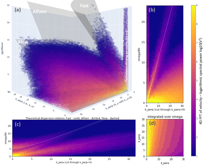
Figure 1: Spatio-temporal (4D FFT) spectrum of run B in the $\omega$ vs. $k_{\perp}$ and $k_{\parallel}$ domain, showing the Fast, Alfvén, Slow components that are indicated by the gray surfaces shown in Panel (a), as well as fluctuations we call “non-waves”. 2D cuts are shown in Panels (b) and (c) to emphasize the three wave branches and the non-wave component. Panel (d) depicts the power distribution in the $k_{\parallel}-k_{\perp}$ plane by integrating the spectrum over all frequencies.

2.2 Mode decomposition Methods

We describe two methods to identify various wave modes in turbulence. The first one is the “spatial-only” method described in Cho & Lazarian (2003); Yang et al. (2018), which uses the velocity output at each time frame to identify the fraction of Alfvén, Fast and Slow modes, according to the polarization features of velocity predicted by linear wave theory. This approach relies on the fact that any spatial variations at any given timeframe can be projected onto three eigenvectors mathematically. The physical interpretation of this approach, however, is a bit unclear. It certainly makes sense physically when the fluctuation amplitudes are small and nonlinear interactions among different modes are not dominant. But for strong MHD turbulence, the nonlinear interactions become important. It is unclear this approach alone can be used to decide the fractions of various wave components.

The other method we used is the spatio-temporal Fourier transform (4D FFT) which allows us to obtain both the spatial and frequency information of variations. By storing the data outputs frequently with sufficient time resolution ($\sim 100$ frames within each $\tau_{A}$ up to $\sim 10~{}\tau_{A}$), we are able to resolve the dispersion relation of linear waves. This ensures that both the high and low frequencies are captured (they are also related to the spatial resolution and box size). To reduce the data volume, we split the 4D Fourier transform into two steps: First, we make 3D spatial FFT for a variable (e.g., velocity), and store the intermediate data in a time series. Second, we perform the fourth (temporal) layer of the spatio-temporal Fourier transform (for individual frequencies) by integrating the intermediate data over time, and save the results in a series of individual frequencies for further analysis. The outcome of these analyses will be spectral power populated within the 4D $\omega-{\bf k}$ volume. This approach has the advantage of assessing whether the Fast, Slow, Alfvénic fluctuations indeed satisfy their respective dispersion relations.

The three eigenmodes delineate three isosurfaces in the $\omega-{\bf k}$ volume. To determine whether certain spectral power belongs to a specific eigenmode, we allow $\pm 10\%$ deviation in $\omega$ for a specific ${\bf k}$ to compensate for two effects. First, there is a well-known issue of spectral leakage in Fourier transform when periodic signals are truncated unevenly (Harris, 1978), which is the case in the temporal dimension. (We employ periodic boundaries in the spatial dimensions.) To suppress the spectral leakage, the Hanning window function is used in the temporal dimension. Second, there is the possible frequency broadening due to nonlinear interactions. We have also tried to use other “width” $\pm 3\%$ and $\pm 40\%$, but the main conclusions do not change qualitatively.

3 Results

We present results from three runs A, B, and C which differ in their turbulence driving: both A and C have only velocity driving (${\bf f_{\rm v}}$) but A has incompressible ($f_{c}=0$) while C has highly compressible driving ($f_{c}=0.9$). Run B has $f_{c}=0$, but with both ${\bf f_{\rm v}}$ and ${\bf f_{\rm B}}$. All simulations use $512^{3}$ resolution. Both A and C have a cubic simulation box of size $2\pi\times 2\pi\times 2\pi$, and B has an elongated box of size $8\pi\times 2\pi\times 2\pi$. All analyses are performed after simulations have reached quasi-steady state, typically after several $\tau_{\rm A}$.

First, we show the outcome of 4D FFT analyses in identifying various waves as depicted in Figure 1. Panel (a) shows the spatio-temporal spectrum of run B with an elongated box in a 3D representation of $\omega$ vs. $k_{x}$ and $k_{y}$ with $k_{z}=0$ for this plot. We note that $k_{\parallel}\simeq k_{x}$ and $k_{\perp}\simeq(k_{y}^{2}+k_{z}^{2})^{1/2}$. It is clear that fluctuations have cascaded to higher $k$ and with finite frequency. Several main features can be identified. The theoretical dispersion planes are marked as gray surfaces for Fast, Alfvén and Slow modes. The vertical feature along $\omega$ axis at small $|{\bf k}|\leq 2$ is due to driving. Panel (b) shows a 2D cut with $k_{x}=0$ in which Fast mode is most easily identified, given their finite frequencies. In this limit, both Alfvén and Slow modes have zero frequency. Panel (c) shows another 2D cut with $k_{\perp}=5$. This brings out all three wave branches (as marked by the three white lines). Panel (d) shows the power distribution in the $k_{\parallel}-k_{\perp}$ plane by integrating the spectrum over all frequencies. This distribution is similar to the previous studies that demonstrate the anisotropic cascade in $k$-space (e.g., Chhiber et al., 2020). Note that, in Panels (b) (c) (d), we have integrated all possible combination of $k_{y}$ and $k_{z}$ for a given $k_{\perp}$ to capture all the spectral power.

It is interesting to see that there is limited amount of power (to be quantified later) in fluctuations that cascade both to higher $k$ and higher $\omega$ and satisfy the dispersion relations for the three eigenmode branches, as most easily seen in Panels (c) and (b). Slow modes tend to cascade further in $k$ than both the Alfvén and Fast modes, as corroborated by Panel (a).

The most prominent feature is the large fraction of fluctuation power not on any of the three wave branches, which is clearly shown by the lower right region in Panel (b) and the regions in-between three wave surfaces in Panel (a). These fluctuations contain finite ${\bf k}$ and finite $\omega$ even though the highest concentration of power tends to be in the low $\omega$ region. We call them the “non-wave” component, which judging from these plots, contains the most amount of power. By inference, most of the power contained in the $k_{\perp}$ cascade shown in Panel (d) resides in this “non-wave” component as well.

Figure 2: Percentage of spectral power derived from the spatial-only mode decomposition (left and middle bars) and spatio-temporal spectra (right bars) for runs A, B, and C. The (shaded) left bars use the whole data cubes where the middle and right bars use data cubes with some excluded regions (see text for details). With the spatio-temporal spectra method, the non-wave component is dominant and the Fast mode fraction is very small (right bars).

Second, we quantify the percentage of spectral power in various components using runs A, B and C, when the evolution of each run has reached quasi-steady state (after $7-10\tau_{A}$). Because it is uncertain how to interpret the power associated with the injection $k-$space, we adopt two approaches. The first is to use outputs including the injection phase space and calculate the percentage of various components using the spatial-only method. We find that the fractions of A/F/S for run A, B, and C are: 0.760/0.223/0.017 (A), 0.628/0.028/0.344 (B) and 0.400/0.206/0.394 (C), respectively. These are represented as the (shaded) left bars in Figure 2. Both the dominance of Alfvén modes and the increasing fraction of Fast modes with compressible driving are consistent with the previous studies (e.g., Makwana & Yan, 2020).

The other approach we used is to exclude certain regions in $k-$space, then use both the spatial-only and the 4D FFT methods to calculate the power fraction in each component. In order to avoid ambiguity, we exclude the following parts from our percentage analysis. First, because the injection $k$ range is dominated by the injection process, we will exclude the fluctuation power with $|{\bf k}|\leq 2$ in all analysis. In run B, this is $\sim 70\%$ of the total spectral power in the simulation. In addition, we also exclude fluctuations with $k_{\parallel}=0$ and $\omega=0$ due to the degeneracy of Alfvén and Slow modes. This is $\sim 3\%$ of the total power. After these modifications to the data outputs, in Figure 2, we compare those derived from the spatial mode decomposition method (middle bars) and spatio-temporal spectrum method (right bars). For the spatial decomposition method, we find the following: the A/F/S fractions are: 0.237/0.003/0.760 (A), 0.425/0.007/0.568 (B) and 0.210/0.137/0.653 (C), respectively. The slow mode actually has the largest fraction among three wave modes using the spatial decomposition method. This is different from the previous results by other groups probably because we excluded the injection range. The Fast mode fraction, being 0.3% and 0.7% for run A and run B is negligible when the driving is incompressible, but becomes a noticeable fraction $14\%$ in run C when the driving is highly compressible, which is expected.

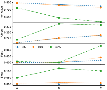
Figure 3: Fractions of spectral power for non-wave, Alfvén, Fast and Slow components (from top to bottom), for run A, B, and C, respectively. These are obtained using the spatio-temporal method only.

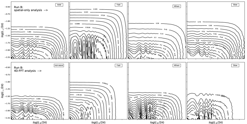
Figure 4: Contours of the second-order structure function of velocity for run B, separately calculated using different components, using the spatial decomposition analysis (top) and the 4D FFT analysis (bottom), respectively.

For the 4D FFT approach, we identify various wave branches according to the theoretical dispersion relations, and we allow 10% deviation in the theoretical frequencies above/below the gray wave surfaces in Figure 1(a) for each wave branch. The remaining power which does not fit within any of the three branches is considered as non-wave. Quantitatively, the percentages of these four components non-wave/A/F/S are: 0.792/0.204/$1\times 10^{-4}$/0.003 (A), 0.762/0.225/$8\times 10^{-7}$/0.013 (B), and 0.729/0.238/0.024/0.009 (C), respectively. They show that the non-wave component is dominant. With regard to wave modes, the Alfvén component has the largest fraction. The Fast mode component is negligible for both A and B but reaches $\sim 2.4\%$ for C.

One key conclusion demonstrated in Figure 2 is that, while the spectral power can always be decomposed into one of three “wave” modes using the spatial decomposition method, when taking into account their frequency behavior, most of these fluctuations do not follow any dispersion relation. Figure 2 also shows that the total fraction in waves using the 4D FFT method is less than $\sim 25\%$. Run B is designed to have the most Alfvénic component by including magnetic injection. Indeed, for both methods, the Alfvén mode fraction in B is higher than either A or C. This driving also generates a finite albeit small fraction of slow waves in run B. Run C is designed to have the most compressible modes, but its Fast mode fraction decreases from $\sim 14\%$ using the spatial decomposition method to $\sim 2.4\%$ using the 4D FFT method.

To test the dependence on the choice of frequency “width”, we also calculate the percentages of spectral power by capturing the power within $\pm 3\%$ and $\pm 40\%$ of theoretical frequency, using data cubes with exclusions as described above. These are summarized in Figure 3. The non-wave/A/F/S components are: for $\pm 40\%$, 0.727/0.218/0.005/0.050 (A), 0.590/0.289/$7\times 10^{-6}$/0.121 (B), and 0.535/0.283 /0.080/0.102 (C); for $\pm 3\%$, 0.795/0.204/$1\times 10^{-4}$/$8\times 10^{-4}$ (A), 0.773/0.224/$2\times 10^{-7}$/0.003 (B), and 0.749/0.236/0.011/0.002 (C), respectively. It can be seen that the overall trends do not change as we vary from $\pm 3\%$ to $\pm 40\%$.

Third, we examine the second-order structure function of various components to further quantify their properties. We calculate the structure functions of individual components in run B obtained using the two mode decomposition methods and use $3\%$ frequency width.

Figure 4 shows the contours of second-order structure function from run B using the spatial-only mode decomposition (top) and the 4D FFT method (bottom). For the top row, we split the Fourier spectral power of the total velocity into Fast, Alfvén, and Slow modes. Then we make the inverse Fourier transform and calculate the second-order structure function of these three modes in real space. Fast modes trend to be isotropic, while Alfvén and Slow modes are elongated, consistent with previous studies (Goldreich & Sridhar, 1995; Cho & Lazarian, 2002, 2003). To avoid double-counting, we exclude the fluctuations with $k_{\parallel}=0$ (where Alfvén and Slow modes are degenerate) and $k_{\perp}=0$ (where Alfvén and Fast modes are degenerated). For the bottom panel, we first identify various wave branches according to the theoretical dispersion relation, allowing 3% deviation in the theoretical frequencies above/below the gray wave surfaces in Figure 1(a) for each wave branch. Then we make 4D inverse Fourier transform and calculate the structure functions for the non-wave, Fast, Alfvén, and Slow components, as shown in the contour plots. We see the general trend that Fast mode appears more isotropic, and the other three components (non-wave, Alfvén, and Slow) are more anisotropic. (The slow component might be too noisy to be accurate.)

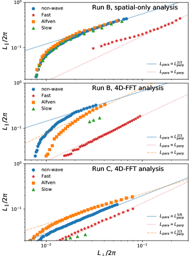
Figure 5: Relationships between $L_{\perp}$ and $L_{\parallel}$ for different components identified in run B (spatial decomposition only), run B (4D FFT method), and run C (4D FFT method).

To further quantify the differences of wave components derived from the two methods, in Figure 5, we plot the relationship $L_{\parallel}\propto L_{\perp}^{q}$ of various components identified in runs B and C. We summarize the power index $q$ as follows: Run B spatial-only: total/A/F/S = $\frac{2}{3}$/$\frac{2}{3}$/1/$\frac{2}{3}$; Run B 4D-FFT: non-wave/A/F/S = $\frac{2}{3}$/1/1/1; Run C spatial-only, total/A/F/S = $\frac{5}{6}$/$\frac{2}{3}$/$\frac{4}{5}$/$\frac{2}{3}$; Run C 4D-FFT, Run C 4D-FFT:non-wave/A/F/S = $\frac{5}{6}$/$\frac{2}{3}$/1/1. (Note that we have added the results for run C using the spatial-only method.)

Taking Figures 4 and 5 together, we can tentatively draw the following conclusions: 1) Using the spatial-only method with incompressible driving, the relations of $L_{\parallel}\propto L_{\perp}^{2/3}$ for the total, Alfvén and Slow components, and $L_{\parallel}\propto L_{\perp}$ for the Fast component, are all the same as those given by previous studies (e.g., Cho & Lazarian, 2003); 2) Using the spatial-only method but with highly compressible driving, the slopes for the total ($5/6$) and Fast mode ($4/5$) components are actually slightly different from the incompressible case ($2/3$ for total and $1$ for Fast); 3) Using the 4D FFT method, for A/F/S components, both run B and C give either the same or slightly steeper slopes from those obtained via the spatial-only method; 4) Using the 4D FFT method, there are differences in the slopes for the non-wave and Alfvén components when comparing run B and C; 5) The Fast component using the 4D FFT method gives slope of $1$ for both run B and C; 6) As a consistency check, for both run B and C, the slopes for the total ($2/3$, $5/6$) and the non-wave component ($2/3$, $5/6$) are the same because they dominate the spectral power using either the spatial-only or the 4D FFT method. These slopes, showing slight variations under different conditions, suggest that additional theoretical and numerical studies are needed to address these differences.

4 Conclusion and Discussion

To understand the nature of MHD turbulence fluctuations in the frequency vs. wavenumber domain in more detail, we have applied both the spatial decomposition method and the spatio-temporal method to examine the properties of MHD turbulence. Particularly, we present results from three simulations, one (run A) with incompressible velocity driving, one (run C) with highly compressible velocity driving, and one (run B) with incompressible velocity and magnetic field driving.

After excluding fluctuations associated with driving and the ($k_{\parallel}=0,~{}\omega=0$) component, we find that: when taking into account the frequency behavior, the majority of the fluctuations cannot fit within any of the Alfvén, Fast and Slow mode branches. We call them the “non-wave” component, which account for about $75-80\%$ of the total power. Furthermore, we find that most of the “non-wave” power is of low frequencies. Similar findings of ultra-low-frequency spectral power were presented in Dmitruk & Matthaeus (2007, 2009), i.e., their “1/f noise”. However, to resolve the “1/f noise” in 4D FFT analysis, it may need an even longer time duration and a larger simulation domain than what we used here, which is beyond the scope of this paper. Observationally, the strong non-wave component is consistent with the results of Bieber et al. (1996) and subsequent work that showed the solar wind admits frequently an 80%-20% decomposition into 2D-slab modes. Theoretically, the nearly incompressible models of MHD predict (for plasma beta $\sim$1 or $<<$ 1) a dominance of 2D over slab fluctuations (Zank & Matthaeus, 1992, 1993; Zank et al., 2017, 2020).

For those fluctuations that fit within one of the wave branches, the Alfvén mode dominates. The Fast mode is essentially negligible in runs with incompressible driving, and becomes $\sim 2.4\%$ in the run with the highly compressible driving (see, e.g., Zhao et al. (2021), for the minority of fast modes in observations).

In addition, we find that the second-order structure functions for different components show differences from those obtained based on the spatial decomposition method.

Because the Fast modes in MHD turbulence have been postulated to play an important role in understanding particle transport and energization, our results here should open up new questions on the existence of these Fast modes and what quantitative roles they could play. Using the spatial decomposition method to identify different wave modes might be too optimistic in concluding the fraction of Fast modes (and compressible modes in general). Instead, we suggest that the “non-wave” component needs to be taken into account in the particle transport and energization processes in MHD turbulence. This will be a subject of our future studies.

We acknowledge the support from a NASA/LWS project under award No. 80NSSC20K0377 and 80HQTR20T0027. H.L., S.D. and X.F. also acknowledge the support by DOE OFES program and LANL LDRD program. Useful discussions with X. Li and F. Guo are gratefully acknowledged. Simulations were carried out using LANL’s Institutional Computing resources.

References

- Andrés et al. (2017) Andrés, N., Clark di Leoni, P., Mininni, P. D., et al. 2017, Physics of Plasmas, 24, 102314, doi: 10.1063/1.4997990
- Armstrong et al. (1995) Armstrong, J. W., Rickett, B. J., & Spangler, S. R. 1995, ApJ, 443, 209, doi: 10.1086/175515
- Bieber et al. (1996) Bieber, J. W., Wanner, W., & Matthaeus, W. H. 1996, Journal of Geophysical Research, 101, 2511, doi: 10.1029/95JA02588
- Brodiano et al. (2021) Brodiano, M., Andrés, N., & Dmitruk, P. 2021, The Astrophysical Journal, 922, 240, doi: 10.3847/1538-4357/ac2834
- Burlaga et al. (2018) Burlaga, L. F., Florinski, V., & Ness, N. F. 2018, ApJ, 854, 20, doi: 10.3847/1538-4357/aaa45a
- Chandran (2005) Chandran, B. D. G. 2005, Phys. Rev. Lett., 95, 265004, doi: 10.1103/PhysRevLett.95.265004
- Chhiber et al. (2020) Chhiber, R., Matthaeus, W. H., Oughton, S., & Parashar, T. N. 2020, Physics of Plasmas, 27, 062308, doi: 10.1063/5.0005109
- Cho & Lazarian (2002) Cho, J., & Lazarian, A. 2002, Physical Review Letters, 88, 245001, doi: 10.1103/PhysRevLett.88.245001
- Cho & Lazarian (2003) —. 2003, Monthly Notices of the Royal Astronomical Society, 345, 325, doi: 10.1046/j.1365-8711.2003.06941.x
- Clark di Leoni et al. (2015) Clark di Leoni, P., Mininni, P. D., & Brachet, M. E. 2015, Physical Review A, 92, 063632, doi: 10.1103/PhysRevA.92.063632
- Cranmer & Ballegooijen (2012) Cranmer, S. R., & Ballegooijen, A. A. v. 2012, The Astrophysical Journal, 754, 92, doi: 10.1088/0004-637X/754/2/92
- Demidem et al. (2020) Demidem, C., Lemoine, M., & Casse, F. 2020, Phys. Rev. D, 102, 023003, doi: 10.1103/PhysRevD.102.023003
- Dermer et al. (1996) Dermer, C. D., Miller, J. A., & Li, H. 1996, ApJ, 456, 106, doi: 10.1086/176631
- Diamond et al. (2005) Diamond, P. H., Itoh, S. I., Itoh, K., & Hahm, T. S. 2005, Plasma Physics and Controlled Fusion, 47, R35, doi: 10.1088/0741-3335/47/5/R01
- Dmitruk & Matthaeus (2007) Dmitruk, P., & Matthaeus, W. H. 2007, Physical Review E, 76, 036305, doi: 10.1103/PhysRevE.76.036305
- Dmitruk & Matthaeus (2009) —. 2009, Physics of Plasmas, 16, 062304, doi: 10.1063/1.3148335
- Eswaran & Pope (1988) Eswaran, V., & Pope, S. B. 1988, Computers and Fluids, 16, 257. http://adsabs.harvard.edu/abs/1988CF.....16..257E
- Galtier (2009) Galtier, S. 2009, Nonlinear Processes in Geophysics, 16, 83, doi: 10.5194/npg-16-83-2009
- Galtier (2018) —. 2018, Journal of Physics A Mathematical General, 51, 293001, doi: 10.1088/1751-8121/aac4c7
- Goldreich & Sridhar (1995) Goldreich, P., & Sridhar, S. 1995, The Astrophysical Journal, 438, 763, doi: 10.1086/175121
- Harris (1978) Harris, F. J. 1978, Proceedings of the IEEE, 66, 51, doi: 10.1109/PROC.1978.10837
- Hitomi Collaboration et al. (2018) Hitomi Collaboration, Aharonian, F., Akamatsu, H., et al. 2018, PASJ, 70, 9, doi: 10.1093/pasj/psx138
- Li & Miller (1997) Li, H., & Miller, J. A. 1997, ApJ, 478, L67, doi: 10.1086/310560
- Lugones et al. (2019) Lugones, R., Dmitruk, P., Mininni, P. D., Pouquet, A., & Matthaeus, W. H. 2019, Physics of Plasmas, 26, 122301, doi: 10.1063/1.5129655
- Makwana & Yan (2020) Makwana, K. D., & Yan, H. 2020, Physical Review X, 10, 031021, doi: 10.1103/PhysRevX.10.031021
- Markovskii & Vasquez (2020) Markovskii, S. A., & Vasquez, B. J. 2020, ApJ, 903, 80, doi: 10.3847/1538-4357/abb99f
- Marsch (1986) Marsch, E. 1986, Astronomy and Astrophysics, 164, 77. http://adsabs.harvard.edu/abs/1986A%26A...164...77M
- Matthaeus & Goldstein (1982) Matthaeus, W. H., & Goldstein, M. L. 1982, J. Geophys. Res., 87, 6011, doi: 10.1029/JA087iA08p06011
- Meyrand et al. (2016) Meyrand, R., Galtier, S., & Kiyani, K. H. 2016, Phys. Rev. Lett., 116, 105002, doi: 10.1103/PhysRevLett.116.105002
- Meyrand et al. (2016) Meyrand, R., Galtier, S., & Kiyani, K. H. 2016, Physical Review Letters, 116, 105002, doi: 10.1103/PhysRevLett.116.105002
- Miller et al. (1996) Miller, J. A., Larosa, T. N., & Moore, R. L. 1996, ApJ, 461, 445, doi: 10.1086/177072
- Schlickeiser (2002) Schlickeiser, R. 2002, Cosmic ray astrophysics / Reinhard Schlickeiser, Astronomy and Astrophysics Library; Physics and Astronomy Online Library. Berlin: Springer. ISBN 3-540-66465-3, 2002, XV + 519 pp. http://adsabs.harvard.edu/abs/2002cra..book.....S
- Stone et al. (2020) Stone, J. M., Tomida, K., White, C. J., & Felker, K. G. 2020, ApJS, 249, 4, doi: 10.3847/1538-4365/ab929b
- Svidzinski et al. (2009) Svidzinski, V. A., Li, H., Rose, H. A., Albright, B. J., & Bowers, K. J. 2009, Physics of Plasmas, 16, 122310, doi: 10.1063/1.3274559
- Yan & Lazarian (2002) Yan, H., & Lazarian, A. 2002, Phys. Rev. Lett., 89, 281102, doi: 10.1103/PhysRevLett.89.281102
- Yang et al. (2018) Yang, L., Zhang, L., He, J., et al. 2018, The Astrophysical Journal, 866, 41, doi: 10.3847/1538-4357/aadadf
- Yang et al. (2019) Yang, L. P., Li, H., Li, S. T., et al. 2019, MNRAS, 488, 859, doi: 10.1093/mnras/stz1747
- Zank et al. (2017) Zank, G. P., Adhikari, L., Hunana, P., et al. 2017, The Astrophysical Journal, 835, 147, doi: 10.3847/1538-4357/835/2/147
- Zank et al. (2017) Zank, G. P., Du, S., & Hunana, P. 2017, ApJ, 842, 114, doi: 10.3847/1538-4357/aa7685
- Zank & Matthaeus (1992) Zank, G. P., & Matthaeus, W. H. 1992, Nearly incompressible fluid dynamics. https://ui.adsabs.harvard.edu/abs/1992sws..coll..587Z
- Zank & Matthaeus (1993) —. 1993, Physics of Fluids A, 5, 257, doi: 10.1063/1.858780
- Zank et al. (2019) Zank, G. P., Nakanotani, M., & Webb, G. M. 2019, ApJ, 887, 116, doi: 10.3847/1538-4357/ab528c
- Zank et al. (2020) Zank, G. P., Nakanotani, M., Zhao, L.-L., Adhikari, L., & Telloni, D. 2020, The Astrophysical Journal, 900, 115, doi: 10.3847/1538-4357/abad30
- Zhang et al. (2015) Zhang, L., He, J., Tu, C., et al. 2015, The Astrophysical Journal, 804, L43, doi: 10.1088/2041-8205/804/2/L43
- Zhao et al. (2020) Zhao, L. L., Zank, G. P., & Burlaga, L. F. 2020, ApJ, 900, 166, doi: 10.3847/1538-4357/ababa2
- Zhao et al. (2021) Zhao, L. L., Zank, G. P., He, J. S., et al. 2021, The Astrophysical Journal, 922, 188, doi: 10.3847/1538-4357/ac28fb