Quantum Orbital Minimization Method for Excited States Calculation on Quantum Computer

Abstract

We propose a quantum-classical hybrid variational algorithm, the quantum orbital minimization method (qOMM), for obtaining the ground state and low-lying excited states of a Hermitian operator. Given parameterized ansatz circuits representing eigenstates, qOMM implements quantum circuits to represent the objective function in the orbital minimization method and adopts a classical optimizer to minimize the objective function with respect to the parameters in ansatz circuits. The objective function has orthogonality constraint implicitly embedded, which allows qOMM to apply a different ansatz circuit to each input reference state. We carry out numerical simulations that seek to find excited states of H_2, LiH, and a toy model consisting of 4 hydrogen atoms arranged in a square lattice in the STO-3G basis with UCCSD ansatz circuits. Comparing the numerical results with existing excited states methods, qOMM is less prone to getting stuck in local minima and can achieve convergence with more shallow ansatz circuits.

Duke]Department of Physics, Duke University Fudan]School of Mathematical Sciences, Fudan University Duke]Department of Mathematics, Duke University Department of Physics, Duke University Department of Chemistry, Duke University

1 Introduction

The development of quantum computing has boomed in recent years. The supremacy of quantum computing is demonstrated by several groups ^{1, 2}. One of the most promising applications for noisy intermediate-scale quantum (NISQ) devices is the variational quantum eigensolver (VQE) under the full configuration interaction (FCI) framework ^{3, 4, 5, 6, 7, 8}. FCI is a quantum chemistry method which discretizes the time-independent many-body Schrödinger equation numerically exactly. The ground state and low-lying excited states are calculated via solving a standard eigenvalue problem, while the problem dimension scales exponentially as the number of electrons in the system. The FCI framework fits naturally into quantum computing. Quantum algorithms for ground state eigensolvers under FCI framework have been extensively developed in past decades ^{9, 10, 11, 12, 13}. Among them, VQE is a quantum-classical hybrid method and has the shortest circuit depth, which makes it the most widely applied ground state quantum eigensolver on NISQ devices. In short, VQE adopts a parameterized circuit as the variational ansatz $\ket{\phi_{\theta}}$ for the ground state. Then the energy function $\expectationvalue*{\widehat{H}}{\phi_{\theta}}$ is minimized with respect to the parameter $\theta$, where $\widehat{H}$ is the Hamiltonian operator.

In addition to the ground state, excited states play an important role in connecting computational results and experimental observations in quantum chemistry. In this paper, we propose a hybrid quantum-classical algorithm, named quantum orbital minimization method (qOMM), to compute the excited state energies as well as the corresponding states under FCI framework.

Existing approaches for excited states on quantum computers could be grouped into two categories: the excited state energy computation and the excited state vector computation.

Excited state energy computation on quantum computer evaluates the excited state energy without explicitly constructing the state vector. Two methods, quantum subspace expansion (QSE) ^{14, 15, 16} and quantum equation of motion (qEoM) ¹⁷, are representatives of this category. Both of them are based on perturbation theory starting from the ground state. They first construct the ground state $\ket{\phi_{GS}}$ via VQE. Then they evaluate the expansion values on single excited states from the ground state $\ket{\phi_{GS}}$, i.e.,

$$A^{p_{2}q_{2}}_{p_{1}q_{1}}=\expectationvalue{\widehat{a}_{q_{2}}^{\dagger}\widehat{a}_{p_{2}}\widehat{H}\widehat{a}_{p_{1}}^{\dagger}\widehat{a}_{q_{1}}}{\phi_{GS}}$$

and

$$B^{p_{2}q_{2}}_{p_{1}q_{1}}=\expectationvalue{\widehat{a}_{q_{2}}^{\dagger}\widehat{a}_{p_{2}}\widehat{a}_{p_{1}}^{\dagger}\widehat{a}_{q_{1}}}{\phi_{GS}}$$

for $\widehat{a}_{p}^{\dagger}$ and $\widehat{a}_{p}$ being creation and annihilation operators. Once these expansion values are available, QSE solves a generalized eigenvalue problem of matrix pencil $(A,B)$ and obtains the refined ground state energy and low-lying excited state energies on the perturbed space of $\ket{\phi_{GS}}$. qEoM adopts these expansion values into the equation of motion expression and obtains the low-lying excited state energies. Double excitations and higher order excitations from the ground state could be further evaluated and included to improve the accuracy of QSE and qEoM. However, including more excitations leads to a much higher computational cost.

Excited state vector computations include a wide spectrum of methods. Folded spectrum method ¹⁸ folds the spectrum of a Hamiltonian operator via a shift-and-square operation, i.e., $\widehat{H}\rightarrow(\widehat{H}-\lambda I)^{2}$, where $\lambda$ is a chosen number close to the desired excited state energy. Then $(\widehat{H}-\lambda I)^{2}$ is used as the operator in VQE method, and an excited state with the energy closest to $\lambda$ is obtained via the optimization procedure in VQE. Witness-assisted variational eigenspectra solver ^{19, 20} adopts an entropy term as the regularizer in the objective function to keep the minimized excited state close to its initial state, where the initial state is set to be an excitation from the ground state. Quantum deflation method ^{21, 22} adopts the overlapping between the target state and the ground state as a penalty term in the objective function to keep the target state as orthogonal as possible to the ground state. The extension to more than one excited state in the quantum deflation method is straightforward. All these methods above have their classical algorithm counterparts. On the other hand, the following two methods use a unique property of quantum computing, i.e., all quantum operators are unitary and orthogonal states after the actions of quantum operators are still orthogonal to each other. Subspace search VQE (SSVQE) ²³ and multistate contracted VQE (MCVQE) ²⁴ apply the same basic ansatz. They first prepare a sequence of non-parameterized mutually orthogonal states, $\ket{\phi_{1}},\ket{\phi_{2}},\dots,\ket{\phi_{K}}$ for $K$ excited states. Then a parameterized circuit $\widehat{U}_{\theta}$ is applied to these states, as $\widehat{U}_{\theta}$ is unitary (implemented on a quantum computer), $\widehat{U}_{\theta}\ket{\phi_{1}},\dots,\widehat{U}_{\theta}\ket{\phi_{K}}$ are mutually orthogonal. Hence we could minimize the objective function

$$\sum_{k}\expectationvalue{\widehat{U}^{\dagger}_{\theta}\widehat{H}\widehat{U}_{\theta}}{\phi_{k}}$$

to obtain approximated ground state and excited states. The energies associated with $\widehat{U}_{\theta}\ket{\phi_{1}},\dots,\widehat{U}_{\theta}\ket{\phi_{K}}$ are usually not ordered. SSVQE further introduces a min-max problem to obtain a specific excited state. Also, in the SSVQE paper, a weighted objective function is employed to preserve the ordering, which will be the version we investigate numerically in our paper below. The MCVQE approach enriches the ansatz by introducing a unitary matrix applied across states in a classical post-processing step, i.e., $\ket{\psi_{k}}=\widehat{U}_{\theta}\sum_{\ell}\ket{\phi_{\ell}}V_{\ell k}$ for $V_{\ell k}$ being the $(\ell,k)$-th entry of a unitary matrix $V$. Hence a standard eigenvalue problem is solved as the post-processing in MCVQE to obtain $V$.

In this paper, we propose to obtain the excited state vector using the objective function in the orbital minimization method (OMM) ^{25, 26},

$$\begin{split}f(\ket{\psi_{1}},\dots,\ket{\psi_{K}})=&2\sum_{i=1}^{K}\expectationvalue{\widehat{H}}{\psi_{i}}\\ &-\sum_{i,j=1}^{K}\innerproduct*{\psi_{i}}{\psi_{j}}\matrixelement{\psi_{j}}{\widehat{H}}{\psi_{i}}.\end{split}$$ (1)

We refer our method as quantum orbital minimization method (qOMM) throughout this paper. An important property of Eq. (1) is that, even though the orthogonality conditions among $\ket{\Psi_{i}}$s are not explicitly enforced, the minimizer of Eq. (1) consists of mutually orthogonal state vectors. For most other methods, the orthogonality condition is explicitly proposed as a constraint in the optimization problem. The implicit orthogonality property allows us to adopt a different ansatz (with regards to either the numerical parameter values, the structure of the ansatz, or both) for each excited state. In this paper, the variational ansatz class that we use is of the form,

$$\ket{\widetilde{\psi}_{k}}=\sum_{\ell=1}^{K}\widehat{U}_{\theta_{\ell}}\ket{\phi_{\ell}}V_{\ell k},$$ (2)

where $\ket{\phi_{1}},\dots,\ket{\phi_{K}}$ are initial states, $\widehat{U}_{\theta_{1}},\dots,\widehat{U}_{\theta_{K}}$ are parameterized circuits with $\theta_{1},\dots,\theta_{K}$ being the parameters, $V_{\ell k}$ is the $(\ell,k)$-th entry of an invertible matrix $V$ that is applied during a classical post-processing step. Such an expression is more general than those used in other excited state vector methods, which typically either apply the same circuit $\widehat{U}_{\theta}$ to all input states or do not apply the classical post-processing matrix $V$. Another feature of Eq. (1) is that the objective function does not include any hyper-parameter (unlike, e.g., the deflation approach), which makes the method easy to use in practice without parameter tuning. Furthermore, this approach shares the same advantages over QSE and qEoM as SSVQE and MCVQE. Namely, the excited states in qOMM are encoded into the objective function of an optimization problem and not as linear combinations of single and double excitations above the ground state in a post-processing step. This allows the method to 1. compute excited states for which triple and higher excitation terms have a non-negligible contribution without calculating higher order reduced density matrices and 2. treat the ground and excited states on the same footing.

Notice that the objective function Eq. (1) includes the evaluation of the state inner product with respect to the Hamiltonian operator and the state inner product, i.e., $\matrixelement*{\phi_{i}}{\widehat{H}}{\psi_{j}}$ and $\innerproduct*{\psi_{i}}{\psi_{j}}$, respectively. In other existing excited state methods, neither of these two are evaluated directly. Given our variational ansatz, we construct quantum circuits to evaluate both inner products, which are essentially inspired by the Hadamard test. When the evaluation of Eq. (1) is available on a quantum computer, we can adopt gradient-free optimizers to minimize the objective function with respect to parameters, $\theta_{1},\dots,\theta_{K}$.

Finally, we include a sequence of numerical results to demonstrate the efficiency and robustness of the proposed method. We test the following chemistry systems using the proposed method on quantum simulators: H_2 and LiH at their equilibrium configurations, H_2 at a stretched bond distance of twice the equilibrium distance, and a toy model consisting of 4 hydrogen atoms arranged in a square at near-equilibrium distances and a stretched bond distance configuration. We observe that qOMM has two major benefits compared to algorithms such as weighted-SSVQE (In this paper, when we refer to SSVQE, we implicitly mean the weighted version of SSVQE that uses one optimization step for finding multiple eigenvalues simultaneously.) that enforce the orthogonality of the input states at every optimization step. 1) Enforcing the mutual orthogonality of the input states through the overlap terms allows for greater flexibility in the choice of ansatz applied to each input state, as well as greater flexibility in the choice of input states. The circuit applied to each input state must be identical in the SSVQE framework in order to enforce orthogonality, whereas qOMM allows us to apply a different ansatz circuit to each input state. 2) The tendency to get stuck in local minima, while not eliminated entirely, is diminished considerably. The first benefit is important because choosing a suitably expressive ansatz for excited states is often more difficult than the ground state VQE problem. In practice, this means that one is often able to use a more shallow and less expressive ansatz circuit; a feature that is crucial for applications on NISQ devices.

The rest of the paper is organized as follows. Section 2 illustrates the circuits we use to evaluate the inner products. The overall method is discussed in Section 3. In Section 4, we apply the method to various chemistry molecules to demonstrate the efficiency of the proposed method. Finally, Section 5 concludes the paper and discusses future work.

2 Inner Product Circuits

In the objective function of qOMM, the inner product of two states and the inner product of two states with respect to an operator are complex numbers. Both the real and imaginary parts are explicitly needed to construct the objective function. If two states are identical, then the inner products can be efficiently evaluated by the well known Hadamard test. We propose quantum circuits for the evaluation of the inner products for the case in which they are different in this section.

To simplify the notations, we consider evaluating $\innerproduct*{\psi}{\phi}$ and $\matrixelement*{\psi}{\widehat{H}}{\phi}$, where $\ket{\psi}$ and $\ket{\phi}$ are given by a unitary circuit acting on $\ket{0}$, i.e., $\ket{\psi}=\widehat{U}_{\theta_{\psi}}\ket{0}$ and $\ket{\phi}=\widehat{U}_{\theta_{\phi}}\ket{0}$. Given the variational ansatz, the inner product $\innerproduct*{\psi}{\phi}=\expectationvalue{\widehat{U}_{\theta_{\psi}}^{\dagger}\widehat{U}_{\theta_{\phi}}}{0}$ can be viewed as the inner product of $\ket{0}$ with respect to the operator $\widehat{O}=\widehat{U}_{\theta_{\psi}}^{\dagger}\widehat{U}_{\theta_{\phi}}$. In principle, the transpose of the ansatz circuit can be constructed. After the ansatz circuit is compiled into basic gates, the transpose of the circuit is the composition of the transposed basic gates in the reverse ordering. Hence $\innerproduct*{\psi}{\phi}$ could be then evaluated using the Hadamard test, which requires the controlled ansatz circuit and the controlled transpose of the ansatz circuit. Instead, we adopt an idea inspired by the Hadamard test, which can be applied to evaluate $\matrixelement*{\psi}{\widehat{H}}{\phi}$ without controlled transpose of the ansatz circuit. In the following, we discuss such two quantum circuits evaluating the inner products in detail.

2.1 $\innerproduct*{\psi}{\phi}$ evaluation

For complex-valued states $\ket{\psi}$ and $\ket{\phi}$, the inner product $\innerproduct*{\psi}{\phi}$ is also a complex number. The evaluation of $\innerproduct*{\psi}{\phi}$ is divided into the evaluations of the real and imaginary parts. We will introduce the circuit for evaluation of the real part of $\innerproduct*{\psi}{\phi}$ in detail, and the circuit for the imaginary part could be constructed analogously.

Figure 1 illustrates the precise quantum circuit used to evaluate the real part of $\innerproduct*{\psi}{\phi}$. Here we list expressions at all five stages as shown in the figure:

$$\Big{(}H\otimes I\Big{)}\ket{0}\ket*{\vec{0}}= \frac{1}{\sqrt{2}}\Big{(}\ket{0}+\ket{1}\Big{)}\ket*{\vec{0}},$$ (S₁)

$$C\mathchar 45\relax\widehat{U}_{\theta_{\phi}}\frac{1}{\sqrt{2}}\Big{(}\ket{0}+\ket{1}\Big{)}\ket*{\vec{0}}= \frac{1}{\sqrt{2}}\Big{(}\ket{0}\ket*{\vec{0}}+\ket{1}\ket{\phi}\Big{)},$$ (S₂)

$$\Big{(}X\otimes I\Big{)}\frac{1}{\sqrt{2}}\Big{(}\ket{0}\ket*{\vec{0}}+\ket{1}\ket{\phi}\Big{)}= \frac{1}{\sqrt{2}}\Big{(}\ket{1}\ket*{\vec{0}}+\ket{0}\ket{\phi}\Big{)},$$ (S₃)

$$C\mathchar 45\relax\widehat{U}_{\theta_{\psi}}\frac{1}{\sqrt{2}}\Big{(}\ket{1}\ket*{\vec{0}}+\ket{0}\ket{\phi}\Big{)}= \frac{1}{\sqrt{2}}\Big{(}\ket{1}\ket{\psi}+\ket{0}\ket{\phi}\Big{)},$$ (S₄)

$$\Big{(}H\otimes I\Big{)}\frac{1}{\sqrt{2}}\Big{(}\ket{1}\ket{\psi}+\ket{0}\ket{\phi}\Big{)}= \frac{1}{2}\Big{(}\ket{0}\big{(}\ket{\phi}+\ket{\psi}\big{)}+\ket{1}\big{(}\ket{\phi}-\ket{\psi}\big{)}\Big{)},$$ (S₅)

where $H$ is the Hadamard gate, $X$ is the Pauli-X gate, $I$ is the identity mapping, $C\mathchar 45\relax\widehat{U}$ is the controlled $\widehat{U}$ gate. Conducting the measurement on the ancilla qubit, we have the probability measuring zero being,

$$\begin{split}\mathbb{P}(\text{measurement}&=0)\\ &=\frac{1}{4}\big{(}\bra{\phi}+\bra{\psi}\big{)}\big{(}\ket{\phi}+\ket{\psi}\big{)}\\ &=\frac{1}{2}+\frac{1}{2}\real\innerproduct*{\psi}{\phi},\end{split}$$ (3)

where $\real(\cdot)$ denotes the real part of the complex number. Hence, if we execute the quantum circuit as in Figure 1 for $M$ shots and count the number of zeros, the $\real\innerproduct*{\psi}{\phi}$ could be well-approximated given $M$ (which will scale as $\mathcal{O}(\frac{1}{\epsilon^{2}})$ for some target accuracy $\epsilon$ due to statistical sampling noise) is reasonably large.

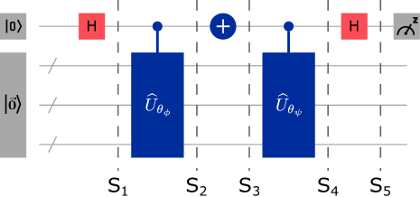
Figure 1: Inner product circuit.

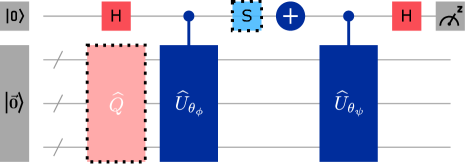
Figure 2: Extended inner product circuit.

The imaginary part of $\innerproduct*{\psi}{\phi}$ could be estimated in a similar way. Notice that the real part in Eq. (3) comes from $\innerproduct*{\psi}{\phi}+\innerproduct*{\phi}{\psi}$. If either $\ket{\psi}$ or $\ket{\phi}$ is replaced by $\imath\ket{\psi}$ or $\imath\ket{\phi}$, then the real part in Eq. (3) corresponds to the imaginary part of the inner product instead. One way to implement the replacement is to add a phase gate on the ancilla qubit after stage Eq. (S₂). The resulting quantum circuit is as that in Figure 2 where the light blue dash box is enabled. We then need to execute the circuit for another $M$ shots to obtain the approximation of $\imaginary\innerproduct*{\psi}{\phi}$.

In addition to variational ansatz $\ket{\psi}=\widehat{U}_{\theta_{\psi}}\ket{0}$ and $\ket{\phi}=\widehat{U}_{\theta_{\phi}}\ket{0}$, we could extend the quantum circuit to variational ansatz $\ket{\psi}=\widehat{U}_{\theta_{\psi}}\widehat{Q}\ket{0}$ and $\ket{\phi}=\widehat{U}_{\theta_{\phi}}\widehat{Q}\ket{0}$, where $\widehat{Q}$ is a common quantum circuit preparing the initial state. If such ansatzes are adopted, we could enable the light pink dash box in Figure 2 such that the circuit $\widehat{Q}$ is applied on $\ket{0}$ as a common circuit. The real and imaginary parts of the inner product are evaluated similarly as before.

2.2 $\matrixelement*{\psi}{\widehat{H}}{\phi}$ evaluation

The Hamiltonian operator considered in this paper is under FCI framework and admits the form,

$$\widehat{H}=\sum_{p,q=1}^{N_{\text{orb}}}h_{pq}\widehat{a}^{\dagger}_{p}\widehat{a}_{q}+\sum_{p,q,r,s=1}^{N_{\text{orb}}}v_{pqrs}\widehat{a}^{\dagger}_{p}\widehat{a}^{\dagger}_{q}\widehat{a}_{s}\widehat{a}_{r},$$ (4)

where $h_{pq},v_{pqrs}$ are one-body and two-body integrals respectively. The Hamiltonian operator $\widehat{H}$, in general, is not a unitary operator. Hence, it cannot be represented by a quantum circuit directly. On the other hand, the excitation operators, $\widehat{a}^{\dagger}_{p}\widehat{a}_{q}$ and $\widehat{a}^{\dagger}_{p}\widehat{a}^{\dagger}_{q}\widehat{a}_{s}\widehat{a}_{r}$, are unitary and can be represented by quantum circuits. The detailed circuits of these excitation operators depend on the encoding scheme. All methods proposed in this paper do not rely on the encoding scheme. The value $\matrixelement*{\psi}{\widehat{H}}{\phi}$ is then calculated as a weighted summation of circuit results,

$$\begin{split}\matrixelement{\psi}{\widehat{H}}{\phi}=&\sum_{p,q=1}^{N_{\text{orb}}}h_{pq}\matrixelement{\psi}{\widehat{a}^{\dagger}_{p}\widehat{a}_{q}}{\phi}\\ &+\sum_{p,q,r,s=1}^{N_{\text{orb}}}v_{pqrs}\matrixelement{\psi}{\widehat{a}^{\dagger}_{p}\widehat{a}^{\dagger}_{q}\widehat{a}_{s}\widehat{a}_{r}}{\phi}.\end{split}$$ (5)

Thus it suffices to consider circuits for the evaluation of $\matrixelement*{\psi}{\widehat{U}}{\phi}$, where $\widehat{U}$ denotes a general unitary operator.

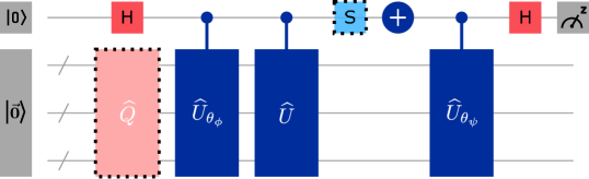
Figure 3: Extended inner product circuit with a unitary gate.

Figure 3 illustrates the circuit for $\matrixelement*{\psi}{\widehat{U}}{\phi}$. This circuit can be understood in the same way as the circuit of $\innerproduct*{\psi}{\phi}$. The value $\matrixelement*{\psi}{\widehat{U}}{\phi}$ can be explicitly written as,

$$\matrixelement{\psi}{\widehat{U}}{\phi}=\Big{(}\bra{0}\widehat{U}_{\theta_{\psi}}^{\dagger}\Big{)}\Big{(}\widehat{U}\widehat{U}_{\theta_{\phi}}\ket{0}\Big{)}=\innerproduct*{\psi}{\widetilde{\phi}},$$ (6)

where the construction circuit for $\ket{\widetilde{\phi}}$ is $\widehat{U}\widehat{U}_{\theta_{\phi}}$. Hence Figure 3 is essentially the circuit in Figure 1 and Figure 2 with a modified constructing circuit for $\ket{\phi}$.

3 Quantum Orbital Minimization Method

Orbital minimization method originates in the field of density functional theory (DFT). The minimization problem admits the following linear algebra form,

$$\min_{X\in\mathbb{C}^{N\times K}}\tr\big((2I-X^{\star}X)X^{\star}\widehat{H}X\big{missing}),$$ (7)

where $X$ is a multi-column vectors with each column denoting a state vector, $\widehat{H}$ is the Hamiltonian matrix, $I$ is the identity matrix of size $K\times K$, and $\tr(\cdot)$ denotes the trace operator. When $\widehat{H}$ is Hermitian negative definite, all local minima of Eq. (7) are of the form ²⁷,

$$X=QV,$$ (8)

where $Q\in\mathbb{C}^{N\times K}$ are $K$ eigenvectors of $\widehat{H}$ associated with the smallest $K$ eigenvalues, and $V\in\mathbb{R}^{K\times K}$ is an arbitary unitary matrix. Substituting Eq. (8) back into Eq. (7), we find that all these local minima are of the same objective value and they are global minima with minimizers consisting of mutually orthogonal vectors. This property has been proven analytically.²⁷ Unlike many other optimization problems for solving the low-lying eigenvalue problem, OMM as in Eq. (7) does not have any explicit orthogonal constraint and the orthogonality in Eq. (8) could be achieved without any orthogonalization step. This property is the key reason for us to investigate the application of Eq. (7) in quantum computing, where explicit orthogonalization is difficult to implement in the presence of hardware and environmental noise. Furthermore, despite the fact that minimizing Eq. (7) is a non-convex problem, its property that all local minimizers are also global minimizers which encode mutually orthogonal vectors in the case where we are minimizing over all possible vectors²⁷ (absent the constraint of vectors expressable as quantum circuits) makes it a compelling objective function to investigate in the quantum setting. The numerical simulations in this work serve to provide some insight into the extent to which these favorable properties in the classical setting carry over to the quantum setting where we are constrained by vectors expressable as quantum circuit ansatzes.

In the quantum computing setting, each column of $X$ is represented by the ansatz $\ket{\psi_{i}}=\widehat{U}_{\theta_{i}}\ket{\phi_{i}}$. By the nature of quantum computing, if quantum error is not taken into account, $\ket{\psi_{i}}$ is always of unit length for all $i$. Hence the $2I-X^{\star}X$ term in Eq. (7) has one on its diagonal. Substituting the variational ansatz into Eq. (7), we obtain the optimization problem for our quantum excited state problem,

$$\min_{\theta_{1},\dots,\theta_{K}}g(\theta_{1},\dots,\theta_{K})$$ (9)

for

$$\begin{split}&g(\theta_{1},\dots,\theta_{K})\\ =&\sum_{i=1}^{K}\matrixelement{\phi_{i}}{\widehat{U}_{\theta_{i}}^{\dagger}\widehat{H}\widehat{U}_{\theta_{i}}}{\phi_{i}}\\ &-\sum_{\begin{subarray}{c}i,j=1\\ i\neq j\end{subarray}}^{K}\matrixelement{\phi_{i}}{\widehat{U}_{\theta_{i}}^{\dagger}\widehat{U}_{\theta_{j}}}{\phi_{j}}\matrixelement{\phi_{j}}{\widehat{U}_{\theta_{j}}^{\dagger}\widehat{H}\widehat{U}_{\theta_{i}}}{\phi_{i}}.\\ \end{split}$$ (10)

If the variational space is rich enough such that vectors in $QV$ as in Eq. (8) can be well-approximated by $\big{\{}\widehat{U}_{\theta_{i}}\ket{\phi_{i}}\big{\}}_{i=1}^{K}$, then qOMM can achieve a good approximation to the global minimum of its linear algebra counterpart Eq. (7). In practice, if we obtain the global minimum value of Eq. (7) for qOMM (though the value is not known in advance), then we are confident that the ansatz is rich enough and the optimizer works perfectly in finding the global minimum for parameters $\theta_{1},\dots,\theta_{K}$. However, we lack the theoretical understanding of the energy landscape of Eq. (9). In part, the dependence of $g$ on $\theta_{1},\dots,\theta_{K}$, like that in the deep neural network, is highly nonlinear and nonconvex. It could be analyzed for some simple ansatz circuit. However, for most complicated circuits, the analysis remains difficult. On the other hand, from the linear algebra point of view, when the variational space is rich enough, we could view the problem as optimizing the vectors $X$ directly in Eq. (7). The nature of quantum computer poses unit length constraints on each column of $X$. Adding extra unit length constraints would dramatically change the energy landscape of the original problem Eq. (7). We defer the theoretical understanding of Eq. (9) to future work. In this paper, we focus on the numerical performance of Eq. (9).

For numerical optimization of the objective function $g$, note that its gradient with respect to a parameter $\theta_{i\alpha}$ is given by

$$\begin{split}\frac{\,\mathrm{d}g}{\,\mathrm{d}\theta_{i\alpha}}=&2\real\matrixelement{\phi_{i}}{\frac{\,\mathrm{d}\widehat{U}^{\dagger}_{\theta_{i}}}{\,\mathrm{d}\theta_{i\alpha}}\widehat{H}\widehat{U}_{\theta_{j}}}{\phi_{j}}-2\real\sum_{\begin{subarray}{c}j=1\\ j\neq i\end{subarray}}^{K}\matrixelement{\phi_{i}}{\frac{\,\mathrm{d}\widehat{U}^{\dagger}_{\theta_{i}}}{\,\mathrm{d}\theta_{i\alpha}}\widehat{U}_{\theta_{j}}}{\phi_{j}}\matrixelement{\phi_{j}}{\widehat{U}_{\theta_{j}}^{\dagger}\widehat{H}\widehat{U}_{\theta_{i}}}{\phi_{i}}\\ &-2\real\sum_{\begin{subarray}{c}j=1\\ j\neq i\end{subarray}}^{K}\matrixelement{\phi_{i}}{\widehat{U}^{\dagger}_{\theta_{i}}\widehat{U}_{\theta_{j}}}{\phi_{j}}\matrixelement{\phi_{j}}{\widehat{U}_{\theta_{j}}^{\dagger}\widehat{H}\frac{\,\mathrm{d}\widehat{U}_{\theta_{i}}}{\,\mathrm{d}\theta_{i\alpha}}}{\phi_{i}},\\ \end{split}$$ (11)

where $\theta_{i\alpha}$ is the $\alpha$-th parameter in $\theta_{i}$. From Eq. (11), we notice that the gradient evaluation requires an efficient quantum circuit for $\frac{\,\mathrm{d}\widehat{U}_{\theta_{i}}}{\,\mathrm{d}\theta_{i\alpha}}$. The existence of such quantum circuits is ansatz dependent. Assume that we can evaluate Eq. (11) for all parameters.Then the update on parameters follows a gradient descent method as

$$\theta^{(t+1)}=\theta^{(t)}-\tau\nabla_{\theta}g(\theta^{(t)}),$$

for $\theta^{(t+1)}$ and $\theta^{(t)}$ being all parameters at $(t+1)$-th and $(t)$-th iteration respectively, and $\tau$ is the stepsize. Since all evaluations of quantum circuits involve randomness, in practice, this amounts to using the stochastic gradient descent method. Other advanced first order methods recently developed in deep neural network literature, e.g., ADAM, AdaGrad, coordinate descent method, etc., could be used to accelerate. These methods could achieve better performance than the vanilla stochastic gradient descent method.

When the gradient circuit is not available, we can adopt zeroth-order optimizers to solve Eq. (9). In this work, we use L-BFGS-B²⁸ as the optimizer, which uses a 2-point finite difference gradient approximation and thus does not require explicit implementation of the circuit for $\frac{\,\mathrm{d}\widehat{U}_{\theta_{i}}}{\,\mathrm{d}\theta_{i\alpha}}$. We find this optimizer to work well in the noiseless simulations we consider here, but we note that other promising candidates for noisy simulations and experimental calculations exist, which could also be used for our proposed objective function. In particular, using simultaneous perturbation stochastic approximation (SPSA) for small molecule VQE calculations has been demonstrated experimentally on superconducting hardware ²⁹ and a quantum natural gradient version of SPSA also exists ³⁰.

When the optimization problem is solved, we will obtain a set of parameters $\theta_{1},\dots,\theta_{K}$ such that $\widehat{U}_{\theta_{1}}\ket{\phi_{1}},\dots,\widehat{U}_{\theta_{K}}\ket{\phi_{K}}$ approximate vectors in $QV$ as in Eq. (8). Numerically, we find that $V$ is very close to an identity matrix, while a post-processing procedure still improves the accuracy of the approximation. The post-processing procedure is slightly different from that in MCVQE. We construct two matrices with their $(i,j)$-th elements being,

$$\begin{split}A_{ij}=\matrixelement{\phi_{i}}{\widehat{U}_{\theta_{i}}^{\dagger}\widehat{H}\widehat{U}_{\theta_{j}}}{\phi_{j}}\text{ and}\\ B_{ij}=\matrixelement{\phi_{i}}{\widehat{U}_{\theta_{i}}^{\dagger}\widehat{U}_{\theta_{j}}}{\phi_{j}}.\\ \end{split}$$ (12)

Then a generalized eigenvalue problem with matrix pencil $(A,B)$ is solved as,

$$AR=BR\Lambda,$$ (13)

where $R$ denotes the eigenvectors and $\Lambda$ is a diagonal matrix with eigenvalues of $(A,B)$ being its diagonal entries. The desired eigenvalues of $\widehat{H}$ are in $\Lambda$ and the corresponding eigenvectors admits $\sum_{j=1}^{K}\widehat{U}_{\theta_{j}}\ket{\phi_{j}}R_{ji}$ for $i=1,\dots,K$. The eigenvector, which is the excited state of $\widehat{H}$, can be explicitly constructed as a linear combination of unitary operators ³¹ on a quantum computer.

qOMM has several unique features compared to existing excited state vector methods. The targets of folded spectrum method ¹⁸ and witnessing eigenspectra solver ^{19, 20} are different from that of qOMM. Quantum deflation method ^{21, 22} addresses the excited states one-by-one, and the optimization problems therein are of different difficulty as that in qOMM. The most related excited state vector methods to qOMM are SSVQE and MCVQE. Since SSVQE and MCVQE are very similar to each other, we focus on the difference among qOMM and SSVQE in this paper. Both the qOMM and weighted SSVQE algorithms ²³ take a set of input states and seek to simultaneously optimize the parameterized circuit and obtain the low-lying eigenvalues and eigenvectors of the Hermitian operator. Both methods achieve their goal via solving a single optimization problem. There are two major differences between them. The first one is how the mutual orthogonality of the eigenvectors is enforced. The construction of the weighted SSVQE objective function ensures that the set of states being evaluated is mutually orthogonal throughout optimization iteration. The proposed qOMM implicitly embeds this constraint into the objective function such that the states being evaluated are only guaranteed to be mutually orthogonal at the global minimum. The first difference leads to the second major difference. SSVQE adopts the ansatz circuits for different states that must admit mutual orthogonal property. Hence, they restrict their ansatz circuits to be a set of identical parameterized circuits acting on mutually orthogonal initial states. qOMM does not constrain the ansatz circuits in this way. qOMM could adopt as its set of parameterized circuits any combination of ansatz circuits that have been tested in the literature, e.g., ansatz circuits in MCVQE ²⁴ and SSVQE ²³, ansatz circuits in deflation method ^{21, 22}, etc. In addition to these ansatz circuits, qOMM could also adopt other ansatz circuits not been tested by excited state methods. In this work, we adopt UCCSD³² as our main ansatz circuit so that the particle number is preserved throughout.

4 Numerical Results

We present the numerical results of our proposed method obtained from a classically simulated quantum computer. We apply it to the problem of finding low-lying eigenvalues of the electronic structure Hamiltonian for near-equilibrium configurations of two different molecules as well the toy model consisting of 4 hydrogen atoms arranged in a square lattice. The numerical tests in this section serve to explore what advantages or disadvantages may arise for each of the qOMM and weighted SSVQE approaches (using weight vectors of the form [$n$, $n-1$, …, $1$] for finding $n$ states) in different situations. Section 4.1 presents the results for H_2 and the hydrogen square model obtained from noiseless simulations. Section 4.2 presents the results obtained from simulating H_2 with a depolarizing noise model. Section 4.3 presents the results for LiH obtained from noiseless simulations.

All codes for these simulations are implemented using the Qiskit ³³ library. The electronic structure Hamiltonians were generated using molecular data from PySCF ³⁴ in the STO-3G basis and mapped to qubit Hamiltonians using the Jordan-Wigner mapping for the noiseless simulations and the Parity mapping for the noisy simulations. The relative accuracies of the results for both methods are calculated by comparing them to their numerically exact counterparts obtained by numerically exact diagonalization of the Hamiltonians. Circuits involved in noiseless qOMM simulations were conducted using Qiskit’s StateVector simulator. Circuits involved in noiseless SSVQE simulations were conducted using Qiskit’s QasmSimulator in conjunction with the AerPauliExpectation method for computing expectation values in order to improve runtime performance. Both of these methods produce ideal, noiseless results. Simulations for finding the energy levels of H2 were performed at an interatomic distance of $0.735$ Angstroms, those of LiH were performed at an interatomic distance of $1.595$ Angstroms, and those of the hydrogen square lattice model were performed at an interatomic distance of $1.23$ Angstroms. Simulation results for the hydrogen square model and H_2 at stretched bond distances can also be found in Appendix A. For the LiH simulations, we freeze the two core electrons to reduce the problem size from 12 qubits to 10 qubits.

Molecule	Algorithm	UCCSD Repetitions
		1-rep	2-rep	3-rep	4-rep	5-rep	6-rep	7-rep
H2 (0.735 Å)	qOMM (3 states)	100%	$-$	$-$	$-$	$-$	$-$	$-$
	SSVQE (3 states)	0%	70%	100%	$-$	$-$	$-$	$-$
H2 (1.47 Å)	qOMM (3 states)	100%	$-$	$-$	$-$	$-$	$-$	$-$
	SSVQE (3 states)	0%	90%	100%	$-$	$-$	$-$	$-$
Hydrogen square (1.23 Å)	qOMM (2 states)	0%	100%	$-$	$-$	$-$	$-$	$-$
	qOMM (3 states)	0%	100%	$-$	$-$	$-$	$-$	$-$
	SSVQE (2 states)	$-$	0%	100%	$-$	$-$	$-$	$-$
	SSVQE (3 states)	$-$	$-$	0%	100%	$-$	$-$	$-$
Hydrogen square (2.46 Å)	qOMM (2 states)	0%	90%	$-$	$-$	$-$	$-$	$-$
	qOMM (3 states)	0%	100%	$-$	$-$	$-$	$-$	$-$
	SSVQE (2 states)	$-$	0%	100%	$-$	$-$	$-$	$-$
	SSVQE (3 states)	$-$	$-$	0%	100%	$-$	$-$	$-$
LiH (1.595 Å)	qOMM (2 states)	0%	100%	$-$	$-$	$-$	$-$	$-$
	qOMM (3 states)	0%	100%	$-$	$-$	$-$	$-$	$-$
	qOMM (4 states)	$-$	100%	$-$	$-$	$-$	$-$	$-$
	qOMM (5 states)	$-$	100%	$-$	$-$	$-$	$-$	$-$
	qOMM (6 states)	$-$	100%	$-$	$-$	$-$	$-$	$-$
	qOMM (7 states)	$-$	100%	$-$	$-$	$-$	$-$	$-$
	SSVQE (2 states)	0%	80%	$-$	$-$	$-$	$-$	$-$
	SSVQE (3 states)	0%	0%	70%	$-$	$-$	$-$	$-$
	SSVQE (4 states)	$-$	$-$	0%	100%	$-$	$-$	$-$
	SSVQE (5 states)	$-$	$-$	$-$	10%	100%	$-$	$-$
	SSVQE (6 states)	$-$	$-$	$-$	$-$	10%	100%	$-$
	SSVQE (7 states)	$-$	$-$	$-$	$-$	$-$	60%	100%

Table 1: The success rate of given problem instances converging to within a relative accuracy of $10^{-5}$ for a given number of UCCSD repetitions using a randomized ansatz parameter initialization.

The set of initial states for both algorithms and all molecular Hamiltonians were chosen to be the Hartree-Fock state and low-lying single-particle excitations above it. For example, if we wish to find three energy levels for 4-qubit H2, in the Jordan-Wigner mapping this would be the set: {$\ket{01}_{\alpha}\ket{01}_{\beta}$, $\ket{01}_{\alpha}\ket{10}_{\beta}$, $\ket{10}_{\alpha}\ket{01}_{\beta}$}. For LiH, this would be the set: {$\ket{00001}_{\alpha}\ket{00001}_{\beta}$, $\ket{00001}_{\alpha}\ket{00010}_{\beta}$, $\ket{00010}_{\alpha}\ket{00001}_{\beta}$}, where the subscript $\alpha$ and $\beta$ denote the spin group . Given that the UCCSD³² ansatz preserves the numbers of spin-up and spin-down, the above choice of initial states constrains these variational quantum algorithms to search only the desired subspace, lessening the computational difficulty and producing physically meaningful results at the same time. For this reason, UCCSD is our ansatz of choice for these simulations. If we wish to find only two energy levels, we would omit the highest-energy state from the set. This choice of the set of states allows us to study two different types of algorithm initializations: one in which all of the ansatz parameters are randomly sampled according to a uniform distribution on $[-2\pi,2\pi)$ and another one in which they are all set to zero. With the random parameter initialization, we can study the robustness of the algorithms with respect to their starting point in the parameter space. With the “zero vector” initialization, the UCCSD ansatz circuit is initialized to the identity and the states after the initial ansatz circuit application remain the Hartree-Fock state and low-lying single-particle excitations above the Hartree-Fock states. For most molecules, these states from Hartree-Fock calculation are good approximations of the ground state and low-lying excited states under FCI. The optimization from the “zero vector” initialization could be viewed as a local optimization and improves the performance of optimizers upon the random initialization. In Qiskit’s implementation of ansatz circuits such as UCCSD, one can increase the expressiveness of the ansatz by repeating the corresponding quantum circuit block pattern $r$ times, which comes at the cost of both the circuit depth and the number of variational parameters increasing by a factor of $r$. In this paper, we refer to an ansatz circuit that consists of the UCCSD circuit block pattern repeated $r$ times as $r$-repetition UCCSD (or simply $r$-UCCSD). We run both algorithms for several different numbers of repetitions in order to account for the fact that the necessary ansatz expressiveness for convergence is not known a priori. Such a study allows us to explore the dependence of convergence success on the circuit depth for each algorithm.

When using a random initialization, we run each algorithm ten times for each setting. In Sections 4.1 and 4.3, for each setting we plot one run roughly representative of the average convergence. In the noisy results in Section 4.2, we plot the run which obtained the lowest objective function convergence. The complete set of all ten runs for all of these simulations are plotted in the appendix and their convergence success rates are summarized in Table 1 for completeness. When using the “zero vector” initialization, we run each algorithm only once. Running the algorithm multiple times for this initialization is neither necessary nor useful in the absence of noise because the outcome is deterministic for a given initial point.

4.1 H2 and Hydrogen square

We begin by presenting the results for the 4 and 8 qubit systems we consider here: H2 and the hydrogen square model. Figure 4 illustrates the convergence of the objective function for each algorithm when attempting to calculate the first three energy levels of the H2 molecule at the equilibrium bond distance.

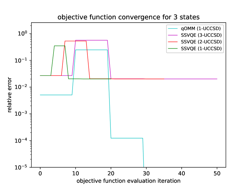
(a) Zero vector initialization

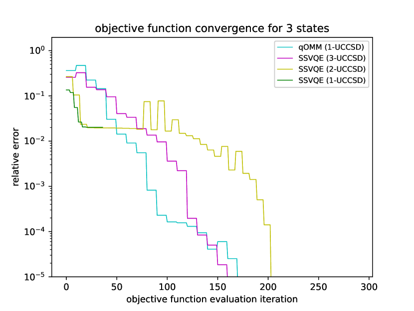
(b) Random initialization

Figure 4: Convergence (noise-free) of the relative error $\frac{\absolutevalue{f_{i}-f_{exact}}}{\absolutevalue{f_{exact}}}$ of qOMM and SSVQE for 3 H_2 states at an interatomic distance of 0.735 Å.

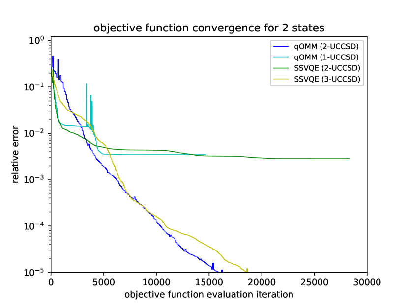
(a) Two states

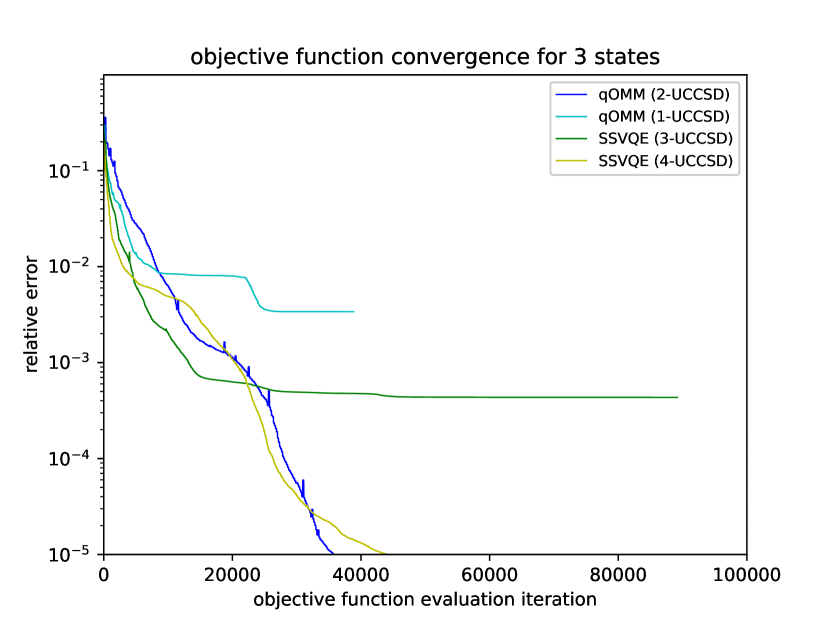
(b) Three states

Figure 5: Convergence (noise-free) of the relative error $\frac{\absolutevalue{f_{i}-f_{exact}}}{\absolutevalue{f_{exact}}}$ of qOMM and SSVQE for the hydrogen square model at an interatomic distance of 1.23 Å using a random parameter initialization.

Figure 4(b) demonstrates how qOMM and SSVQE both converge to the global minimum, but notably, SSVQE cannot do so with just 1-repetition UCCSD, requiring two repetitions in order to converge to within a relative accuracy of $10^{-5}$. The success rate is further reported in Table 1. Figure 4(a) illustrates an attempt to solve the same problem, except the ansatz parameters are all initialized to zero. In this instance, we see that qOMM converges more quickly by a factor of roughly 5 compared to its random initialization counterpart, while SSVQE gets stuck in a local minimum and does not converge regardless of the ansatz circuit depth used. In both figures and all later convergence figures in this paper, we depict the convergence curve as the relative error (defined as $\frac{\absolutevalue{f_{exact}-f_{measured}}}{\absolutevalue{f_{exact}}}$) against the number of the objective function evaluations, which is considered the most expensive operation in VQE-type algorithms. The L-BFGS-B implementation used in this paper uses a 2-point finite difference method such that each parameter is perturbed slightly from a given reference point common to all of them. Thus for an $n$-parameter objective function, $n+1$ function evaluations are required for each parameter update step in order to estimate the gradient. Hence, in all convergence figures, we observe stair-like curves of width $n+1$.

Figure 5 illustrates the convergence results for the hydrogen square lattice at an interatomic distance of $1.23$ Angstroms. We can see from these figures that similarly to H_2, the difference between SSVQE and qOMM is primarily in the number of UCCSD repetitions needed to converge. When calculating 2 states, qOMM requires 2-UCCSD whereas SSVQE requires 3-UCCSD. When calculating 3 states, qOMM still requires only 2-UCCSD, whereas SSVQE requires 4-UCCSD. These observations are further tabulated in Table 1.

4.2 Noisy H_2 simulations

We now run H_2 simulations in the presence of a classically simulated noise model on Qiskit’s AerSimulator. Each one-qubit gate in the circuit is modelled as being accompanied by a local depolarizing channel with some probability of error $p_{error}$. Two-qubit gates are accompanied by a tensor product of two local depolarizing channels acting on each qubit. No error mitigation strategies are employed. We use the Parity mapping in order to use symmetry considerations to reduce the H_2 Hamiltonian to a 2 qubit representation³⁵. We construct ansatzes for each algorithm using the circuit block pattern shown in Figure 6.

@C=1em @R=.7em & R_y(θ_0) R_z(θ_2) 1 R_y(θ_4) R_z(θ_6)
R_y(θ_1) R_z(θ_3) R_y(θ_5) R_z(θ_7)

Figure 6: Base circuit block pattern used for noisy H_2 simulations.

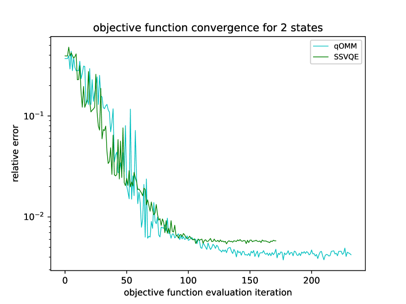
(a) Two states

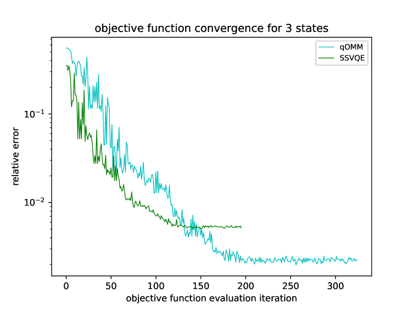
(b) Three states

Figure 7: Convergence of the relative error $\frac{\absolutevalue{f_{i}-f_{exact}}}{\absolutevalue{f_{exact}}}$ of qOMM and SSVQE for H_2 at an interatomic distance of 0.735 Å, where each circuit gate is modelled as having a probability of local depolarizing error $p_{error}=0.001$.

This pattern can be repeated an arbitrary number of times to construct increasingly expressive ansatzes in the same way that the number of UCCSD repetitions was varied in the noiseless simulations. The Qiskit compiler is used to compile all circuits to the set of basis gets consisting of $R_{z}$, $R_{y}$, CNOT, $\sqrt{X}$, and the identity. For all problem instances, we use the minimum number of repetitions necessary to converge in the absence of noise in order to ensure that we are not simply measuring the ability of the ansatz to represent the global minimum. This corresponds to one repetition for qOMM and two repetitions for SSVQE. We use COBYLA as the classical optimization subroutine. This optimizer is more suitable for noisy simulations than L-BFGS-B due to its lack of a need to calculate gradient information. $10^{6}$ circuit samples are used to evaluate all inner product terms and expectation values. $p_{error}$ is set to $10^{-3}$. Both SSVQE and qOMM are run ten times with randomly initialized parameters. The convergence of the runs which achieved the lowest objective function values are given in Figure 7. The results for all ten runs are given in Appendix A. We can see from these figures that both SSVQE and qOMM demonstrate a robustness to noise, although they do not achieve the same accuracy as the noiseless results.

4.3 LiH

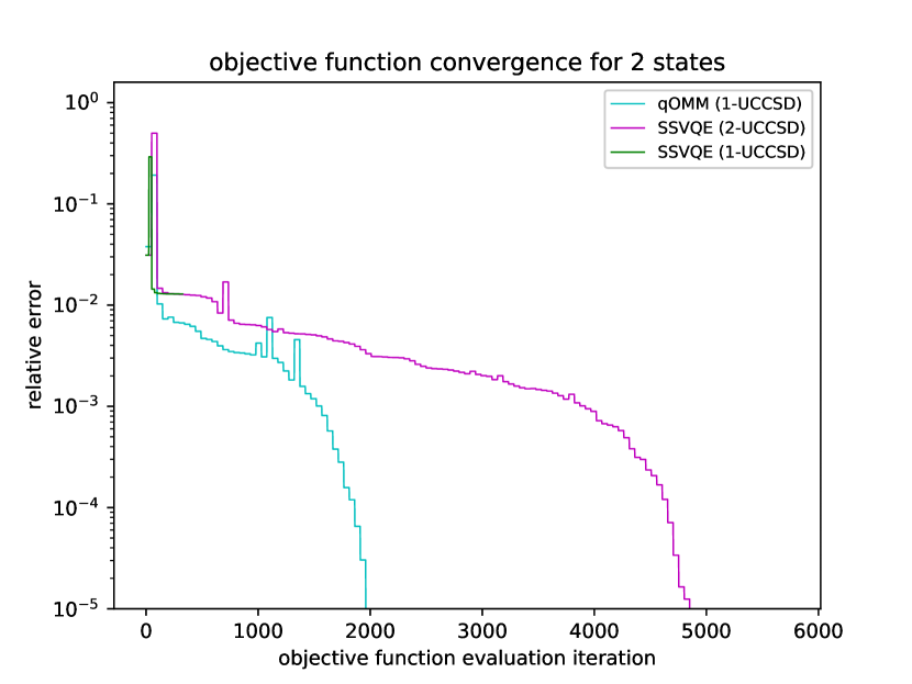
(a) Two states (zero vector initialization)

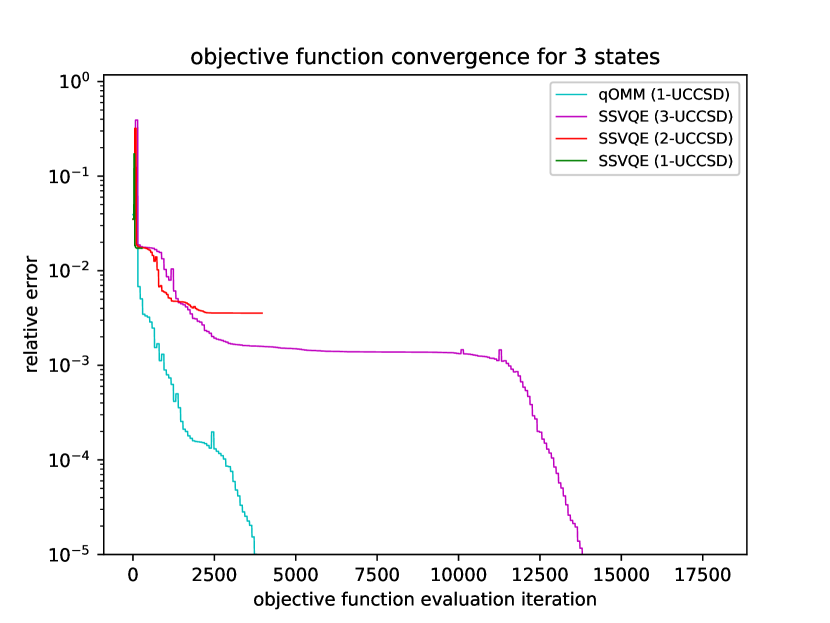
(b) Three states (zero vector initialization)

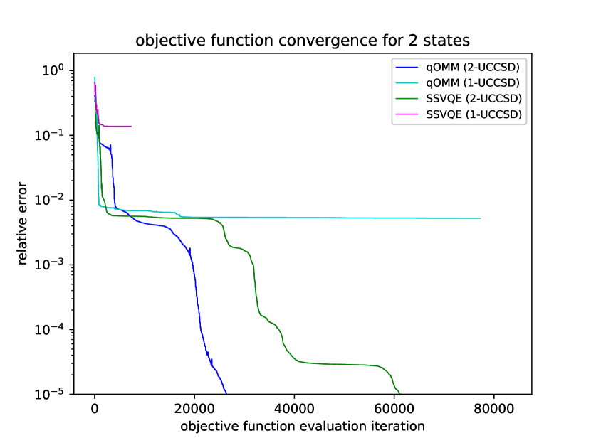
(c) Two states (random initialization)

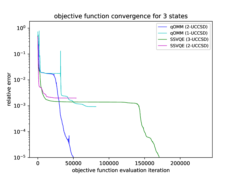
(d) Three states (random initialization)

Figure 8: Convergence of the relative error $\frac{\absolutevalue{f_{i}-f_{exact}}}{\absolutevalue{f_{exact}}}$ of qOMM and SSVQE for LiH.

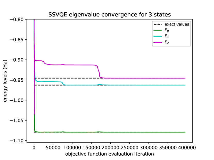
Figure 9: Convergence of the first three energy levels of LiH for SSVQE using a random parameter initialization.

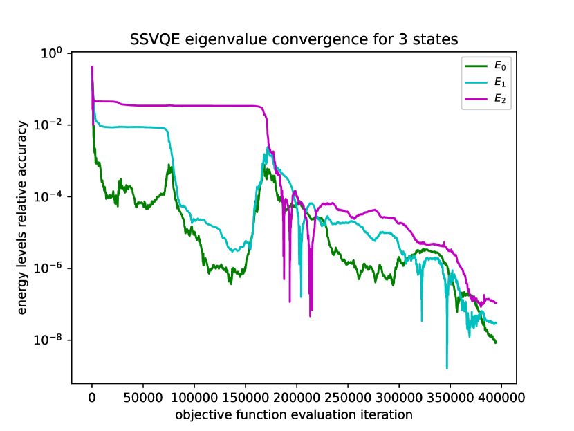
Figure 10: Relative accuracy $\frac{\absolutevalue{E_{n,i}-E_{n,exact}}}{\absolutevalue{E_{n,exact}}}$ of the convergence of the first three energy levels of LiH for SSVQE using a random parameter initialization.

We now present the results for the 10-qubit system we consider here: LiH. Figure 8 illustrates the convergence of the objective function for both algorithms with various UCCSD ansatzes when calculating up to the first three energy levels. We can see from Figure 8(c) that when the ansatz parameters are randomly initialized, both algorithms demonstrate the ability to converge within an accuracy of $10^{-5}$, but require 2-repetition UCCSD to do so. From Figure 8(a) we can see that when all of the parameters are initialized to zero, both algorithms converge to within a relative accuracy of $10^{-5}$ much more quickly than their randomly initialized counterparts. Notably, qOMM requires only 1-repetition UCCSD to achieve this convergence, while SSVQE requires two repetitions. When three states are calculated, qOMM can achieve a convergence below $10^{-5}$ with 2-repetition UCCSD, whereas SSVQE requires three repetitions. From Figure 8(b) we can see that when the ansatz parameters are all initialized to zero, both algorithms quickly converge to the global minimum. Notably, qOMM requires only 1-UCCSD repetition with this initialization. When attempting to find larger numbers of states, we can see from Table 1 that qOMM can converge with 2-UCCSD for all numbers of states considered, whereas SSVQE requires an increasing number of ansatz repetitions to find increasing numbers of states. In the following, we discuss the numerical results on LiH mainly from three perspectives: convergence plateau, initialization, and ansatz circuit depth.

Convergence Plateau. In many of the LiH convergence plots we show here, both qOMM and SSVQE initially converge at a rapid rate but then hit a plateau and stall the convergence until they escape from the “bad” region of the energy landscape. As long as the algorithm escapes from the “bad” region, the convergence rate resumes being rapid. These “bad” regions of the energy landscape (regardless of what their nature may be) seem to be the main obstacle for the convergence of both algorithms, which is more severe to SSVQE. Studying this apparent feature of the energy landscape may provide some insight as to how both algorithms may be improved and what limitations are inherent to the construction of the cost functions. From a numerical linear algebra point of view, such a convergence behavior is not very surprising. The objective function in SSVQE is convex, while with the consideration of the orthogonality constraint and the parameterization of the ansatz circuits, the energy landscape of SSVQE becomes non-convex. On the other hand, the objective function of qOMM, by itself, is non-convex but has no spurious local minima ^{27, 36, 37}. When the parameterization of the ansatz circuits is taken into consideration, the energy landscape of qOMM is non-convex and could have spurious local minima. For non-convex energy landscapes, usual optimizers, including L-BFGS-B, are efficient in a neighborhood of local minima whereas, around strict saddle points, without second-order information, the optimizers could stall there for a long time. From a practical point of view, we can further investigate the convergence of each eigenvalue. Since the issue is more severe for SSVQE, we focus on the SSVQE rather than qOMM. The construction of the SSVQE objective function allows us to obtain the estimated values for each eigenvalue at every function evaluation (in addition to the objective function as a whole) at a negligible additional computational cost. This allows us to gain some intuition as to why the SSVQE objective function convergence is observed to plateau in many of the LiH runs before steeply converging below a relative accuracy of $10^{-5}$. In Figure 9 and Figure 10, we plot the eigenvalues and their relative accuracies, respectively, for one of the ten randomly-initialized SSVQE runs. We can see from Figure 9 that while $E_{0}$ converges rapidly, the convergence of $E_{1}$ and $E_{2}$ plateau and do not converge for many more function evaluations. From Figure 10 we can see that $E_{1}$ does not escape from its plateau until the accuracy of $E_{0}$ is sufficiently decreased. This is followed by the accuracies of $E_{0}$ and $E_{1}$ increasing together. $E_{2}$ does not escape from its plateau until the accuracies of $E_{0}$ and $E_{1}$ are both sufficiently decreased, after which the accuracies of all three energy levels collectively increase, allowing the objective function to converge to its global minimum. While we only illustrate this for one of the ten runs, we observe that this qualitative behavior is typical for the other nine runs. Besides the non-convexity reason from objective functions, other reasons for this behavior could be related to two aspects of the weighted sum nature of the SSVQE algorithm. First, the same ansatz circuit is applied to all input states, meaning any change in the parameters has a direct impact on all the expectation value terms simultaneously. Second, the energy levels contribute unequally to the overall cost function, with the lower energy levels contributing more than the higher energy levels, an effect that becomes more pronounced due to the presence of the weight vector. Because qOMM enforces orthogonality (at the global minimum) through its overlap terms, the energy expectation value terms are associated with different independent parameter values. This means that changes in parameters that directly affect one of the energy expectation value terms in Eq. (1) do not directly change the others. They only change the overlap terms. This affords qOMM a flexibility that allows it to spend much fewer iterations escaping from the “bad” landscape regions. From Figure 8(b) and Figure 8(a) we see that starting with a good initial guess can reduce this effect, resulting in significantly improved convergence.

We also briefly note that although we have chosen to measure convergence speed in terms of the number of calls to the objective function, another valid measure of convergence speed would be the total number of optimization iterations if it can be assumed that one can parallelize multiple calls to the objective function. This is because one optimization iteration can require multiple calls to the objective function. In the noiseless results we have presented here, each optimization iteration of the L-BFGS-B optimizer requires $n$+1 calls to the objective function for $n$ total parameters. For problem instances we have presented here where qOMM has more parameters than SSVQE, the speedup of qOMM over SSVQE would be even greater by this measure. For instance, in Figure 8(d), qOMM with 2-UCCSD has 144 total parameters and SSVQE with 3-UCCSD has 72.

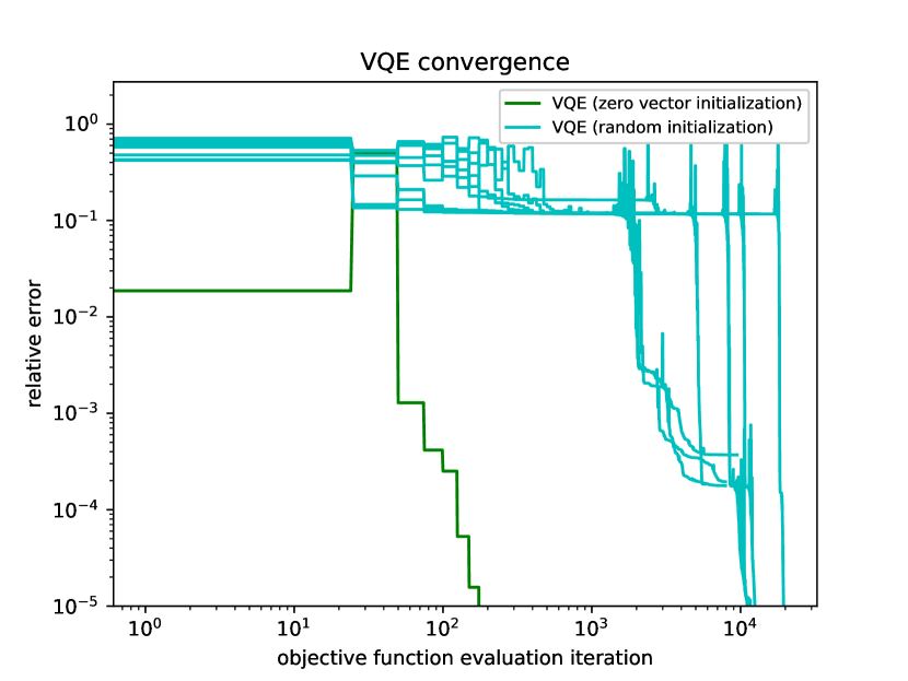
Figure 11: Convergence of the relative error $\frac{\absolutevalue{E_{0,i}-E_{0,exact}}}{\absolutevalue{E_{0,exact}}}$ of VQE for the ground state problem of LiH using a random parameter initialization

Initialization. Initialization plays an important role in the convergence for both qOMM and SSVQE. Even for the corresponding VQE ground state problem with 1-repetition UCCSD, as in Figure 11, random parameter initialization on average converges in about 100 times more objective function evaluations than the zero vector parameter initialization. Both initializations in Figure 11 converge to a relative error $10^{-5}$. In excited state computing, the two different initialization strategies for both qOMM and SSVQE not only differ in the number of iterations but also differ in the convergence results. Comparing Figures 8(a) and 8(c), for SSVQE with 2-repetition UCCSD, random parameter initialization converges more than ten times slower than that of zero vector parameter initialization. A similar result can be observed in Figures 8(b) and 8(d) for SSVQE with 3-repetition UCCSD. Besides the difference in the number of iterations, optimization starting from random parameter initializations sometimes cannot find the global minima, as can be seen from Table 1. Overall, in all results included in this paper, zero vector parameter initializations outperform their random parameter initialization counterparts for both algorithms. However, we still include numerical results for random parameter initializations to demonstrate the different performance between qOMM and SSVQE. This is because the zero vector initializations initialize the states to be excitations from Hartree-Fock states and only work for a limited number of low-lying states. If more excited states are needed, the zero vector initialization could even be a bad initialization, which is due to the fact that the excitation energies from Hartree-Fock may not be in the consistent order with that of FCI excitation energies. This "zero vector" initialization is demonstrated primarily not to advocate for its use as a scalable initialization strategy, but to illustrate what the improved convergence could look like if it can be assumed that one has a reasonable initialization strategy. The flexibility of variational ansatzes in qOMM would have another advantage when many excited states are needed. In qOMM, we could use zero vector parameter initialization for a few states and random parameter initialization for the remaining states without known good initializations. Such a mixed initialization strategy could avoid being trapped in bad local minima and benefit from the fast convergence of those states with zero vector parameter initialization. SSVQE, unfortunately, cannot use such a mixed initialization strategy due to the implicit orthogonality among initialized states. This motivates further investigation into developing and benchmarking initialization strategies more sophisticated than the ones we consider in this work. For example, the MCVQE paper²⁴ proposes an efficient quantum circuit implementation of CIS states for excited state initializations. This initialization would likely improve the convergence results of the simulations for both qOMM and SSVQE presented in this paper. Furthermore, because the optimization stage of MCVQE can be seen as a special case of SSVQE that uses a CIS initialization and an equal weighting of the states, performing analogous simulations using a CIS initialization would offer insight into how the convergence of qOMM compares to that of MCVQE. The approach of using chemically-motivated initializations inspired from classical computational chemistry is likely to further improve the convergence of algorithms such as qOMM and SSVQE. The main challenge in this approach is that high level chemically-inspired initializations require efficient low-level circuit implementation, which is highly non-trivial.

Ansatz Circuit Depth. Based on our numerical results, increasing the ansatz circuit depth, i.e., increasing the repetition in UCCSD, has two major impacts. First, the expressiveness increases as the ansatz circuit depth increases. In the ground state VQE, as in Figure 11, 1-repetition UCCSD is sufficient for the ansatz to approximate the ground state to chemical accuracy. When two states of LiH are needed, 1-repetition UCCSD, as in Figure 8, is not able to simultaneously approximate the ground state and the first excited states, whereas 2-repetition UCCSD is able to. From the qOMM results in Figure 8(a), we know that 1-repetition UCCSD is able to approximate the ground state and the first excited state. When three states are needed, as in Figure 8(b), we need 3-repetition UCCSD to simultaneously approximate three states. Again, 1-repetition UCCSD is still able to approximate any of these three states. More generally, 2-UCCSD is sufficient for all LiH cases studied when using qOMM, whereas SSVQE requires $n$-UCCSD in order to reliably find $n$ states. The results for the hydrogen square model in Figure 5 demonstrates a similar pattern, except the situation is more severe for SSVQE, which requires more than $n$-UCCSD for finding $n$ states. A more detailed analytical description of the ability of the UCCSD ansatz to simultaneously represent an increasing number of excited states as the number of repetitions is increased is not yet known. qOMM could adopt many UCCSDs, UCCSD with many repetitions, or a mixture of them as its variational ansatz. SSVQE, however, could only benefit from increasing the repetitions in UCCSD. The second impact of ansatz circuit depth relates to optimization. Another field full of non-convex optimization and parametrized ansatz is the deep neural network. An interesting theoretical result ³⁸ therein shows that enlarging the parameter space, i.e., increasing the number of parameters, would make the optimization problem easier, i.e., the energy landscape would be full of the approximated global minimum. Although we have not established similar results for quantum ansatz circuits, we observe the behavior from our numerical results. In Figure 8(b), 1-repetition UCCSD is able to characterize the three states for LiH using qOMM. However, all ten random parameter initializations got stuck as can be seen in Table 1. As we increase the circuit depth from 1-repetition to 2-repetition UCCSD, qOMM rapidly converges to a global minimum for all ten random parameter initializations.

We conclude this section by discussing the circuit depth involved in calculating the inner product terms in the qOMM objective function. Currently, the only method we are aware of that involves running the circuit in Figure 1. At a minimum, the inner product circuit will incur a circuit depth twice that of the original ansatz. There will be additional circuit depth due to the need to compile controlled versions of the ansatz to the finite basis gate set of the machine. The extent of this additional depth compared to the original ansatz will depend on a number of factors including the basis gate set and qubit connectivity of the hardware, the choice of ansatz, and the efficiency of the compilation algorithm used. We can give some intuition for the circuit depths involved for the particular systems we studied here for a particular basis gate set. Using the Qiskit compiler, the gate depth for the 1-UCCSD ansatz used in our LiH simulations is approximately 1400 gates when compiled to the basis gate set consisting of $R_{z}$, $\sqrt{X}$, $X$, CNOT, and the identity. The corresponding circuit depth for computing the inner product terms is approximately 19600 gates. These counts would be scaled roughly by a factor of $n$ for $n$-UCCSD. This underscores the importance of future work that addresses how to reduce these gate counts. In particular, finding (if they exist) more efficient implementations of the inner product computations will be important for the applicability of qOMM in the NISQ era. We emphasize that while there are several known subroutines for computing the overlap of two states for other applications such as quantum machine learning³⁹, these generally compute real quantities of the form $\absolutevalue{\bra{\psi_{1}}\ket{\psi_{2}}}$, whereas for qOMM we need the full complex quantity $\bra{\psi_{1}}\ket{\psi_{2}}$. The observation that SSVQE appears to require an increasingly expressive ansatz for increasingly larger systems and an increasing number of states is also a concern. Future work that addresses how to mitigate this effect will be important for the applicability of SSVQE in the NISQ era. In particular, it has been shown that certain conditions can induce cost function landscapes with gradient magnitudes that vanish exponentially (i.e. barren plateaus) with the number of qubits, rendering convergence infeasible. This has been shown to occur in instances where one uses a hardware-efficient ansatz in combination with a non-local cost function⁴⁰ and in the presence of noise when one uses an ansatz with circuit depth that scales linearly or faster with the number of qubits.⁴¹. Because both of these types of barren plateaus worsen with increasing circuit depth, the extent to which the two methods studied in this paper are susceptible to this effect will likely depend on how the circuit depth required for each algorithm to converge scales with increasing problem size. Such an investigation would require the simulation of larger chemical systems and would be an interesting direction of future research. We also note that there are various strategies that could be employed to facilitate the study of larger systems by representing the active space with as few qubits as possible, effectively delaying the onset of barren plateaus. A simple, well-known example of this idea was used in this work when we froze the two core orbitals in LiH to reduce the problem size from 12 qubits to 10. Another strategy would be to optimize the basis set under a fixed qubit budget, as is done in OptOrbFCI in the context of classical computational chemistry⁴². Generalizing this work to quantum variational algorithms such as VQE, SSVQE, and qOMM will be the topic of future work.

5 Conclusion

In this work we have proposed a method which can calculate the low-lying eigenvalue/eigenstate pairs of a Hermitian operator on quantum hardware. We have classically simulated the algorithm for three different electronic structure Hamiltonians: H2, LiH, and the hydrogen square lattice. We have compared it to SSVQE, another algorithm with the same goal, but one which enforces the orthogonality of the input states explicitly at every optimization step. We showed that a small problem such as H2 is not difficult enough to meaningfully distinguish any differences in performance for these two approaches when using a random initialization strategy, but when one compares them to a more moderately-sized problems such as 10 qubit LiH, noticeable differences in performance begin to emerge. In this scenerio, qOMM converges with fewer objective function evaluations and with a less expressive ansatz in all but one of the simulations considered here. Each of these methods incurs additional circuit depth beyond the ground state problem that should be addressed by future works in order to increase their applicability in the NISQ era. This corresponds to finding more efficient methods for computing the inner product terms in qOMM and reducing the ansatz circuit depth needed for SSVQE to converge efficiently. One potential direction for attempting to improve SSVQE would be to investigate the extent to which incorporating adaptive ansatz strategies ^{43, 44, 45} would alleviate this apparent feature of SSVQE. These methods were developed in order to find depth-efficient ansatz circuits for problem instances for which doing so by manual heuristic guesswork is difficult. This is precisely the problem from which we observed SSVQE to suffer in this work. qOMM could benefit from these methods as well. Additionally, one could investigate whether or not modifying the SSVQE weight vector to adaptively change over the course of the optimization could mitigate the objective function plateau effect we observed in our simulations.

The LiH simulations demonstrate that in the context of these types of excited states methods, even a crude initialization strategy can greatly reduce not only the number of optimization iterations needed to converge, but also the circuit depth needed to do so. Another potentially interesting topic would be to develop and benchmark more powerful and versatile initialization strategies that are taylored specifically to these excited states methods. This would also improve the applicability of these methods in the NISQ era.

The work is supported in part by the US National Science Foundation under award CHE-2037263 and by the US Department of Energy via grant DE-SC0019449.

Appendix A Additional Convergence Plots

Here we provide all ten runs for each of the randomly initialized tests for which only one run was shown in Section 4. We also provide some additional tests such as H_2 and the hydrogen square model at stretched bond distances and up to 7 states of LiH. The success rates for the noise-free simulations are summarized in Table 1 in Section 4.

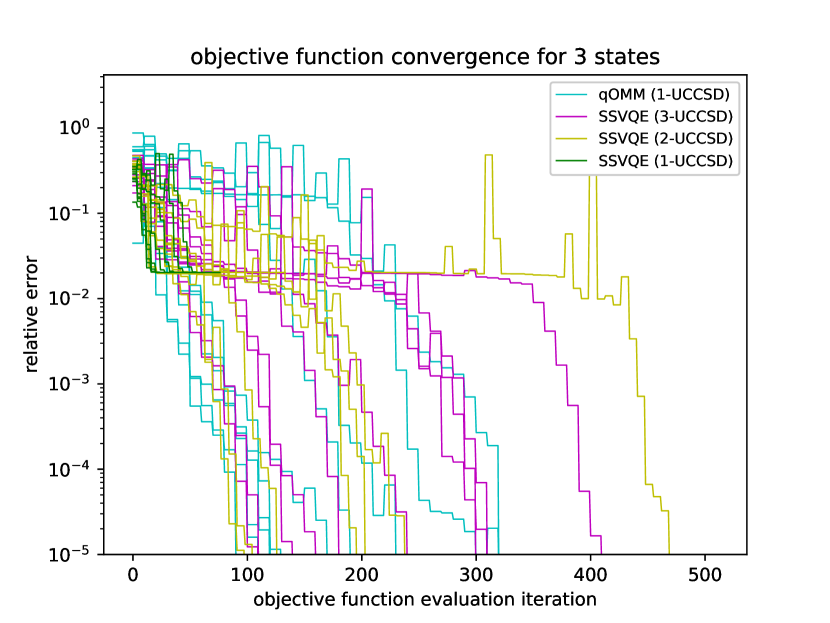
(a) 0.735 Å bond distance

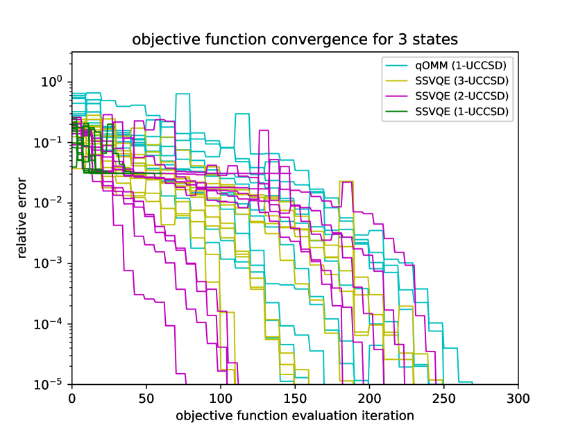
(b) 1.47 Å bond distance

Figure 12: Convergence of the relative error $\frac{\absolutevalue{f_{i}-f_{exact}}}{\absolutevalue{f_{exact}}}$ of qOMM and SSVQE for H_2 using a random parameter initialization.

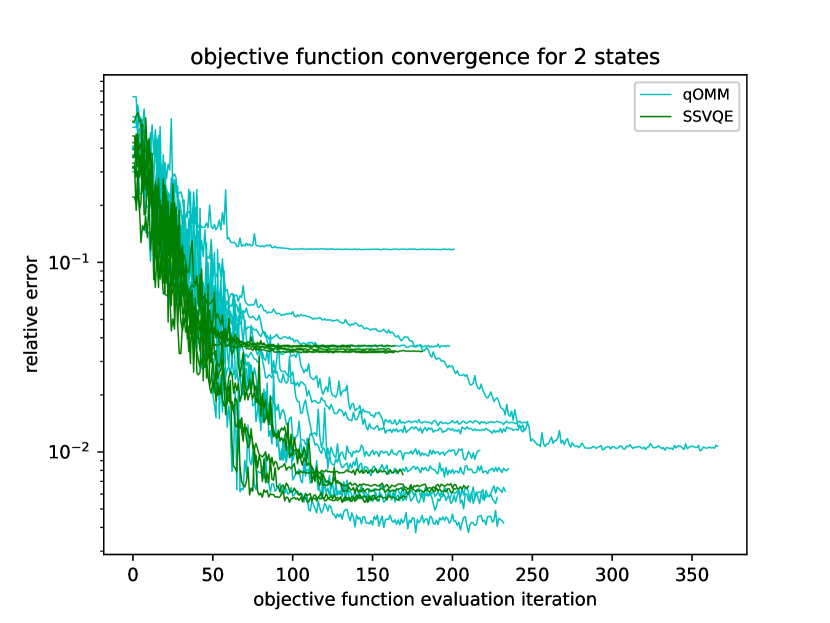
(a) Two states

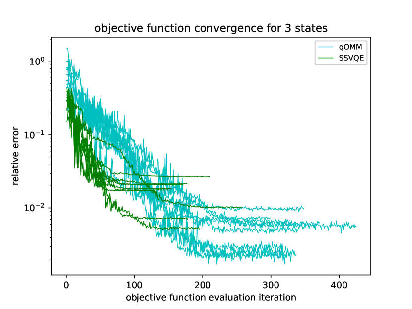
(b) Three states

Figure 13: Convergence of the relative error $\frac{\absolutevalue{f_{i}-f_{exact}}}{\absolutevalue{f_{exact}}}$ of qOMM and SSVQE for H_2 at an interatomic distance of 0.735 Å, where each circuit gate is modelled as having a probability of local depolarizing error $p_{error}=0.001$.

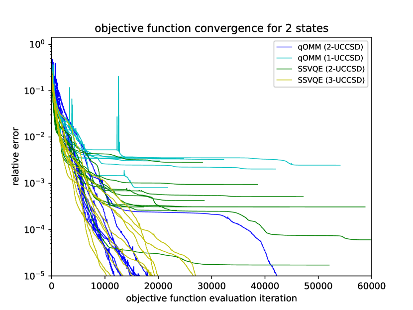
(a) Two states

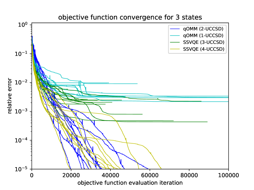
(b) Three states

Figure 14: Convergence of the relative error $\frac{\absolutevalue{f_{i}-f_{exact}}}{\absolutevalue{f_{exact}}}$ of qOMM and SSVQE for the hydrogen square model at an interatomic distance of 1.23 Å using a random parameter initialization.

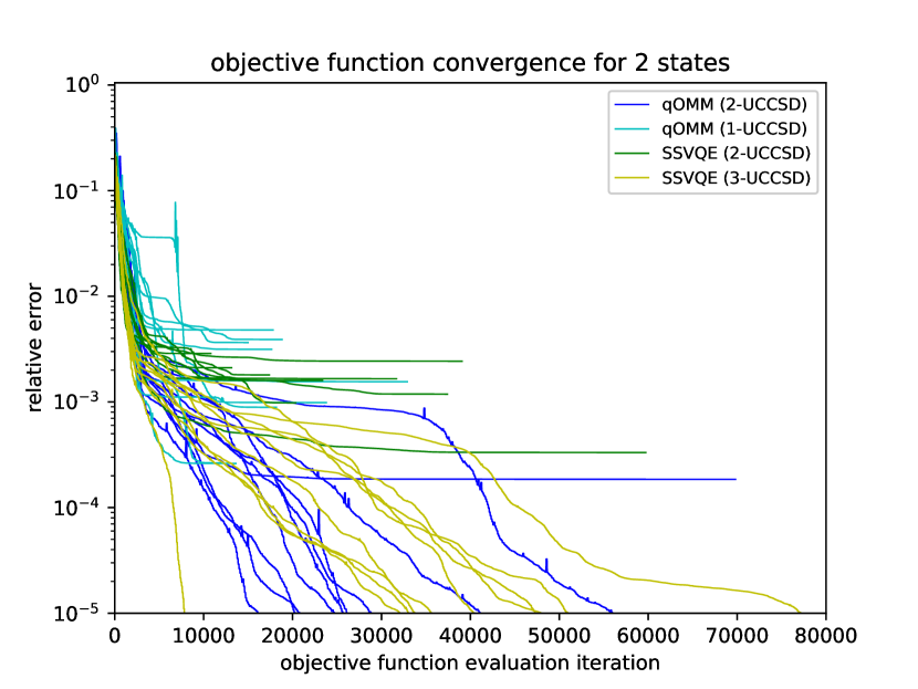
(a) Two states

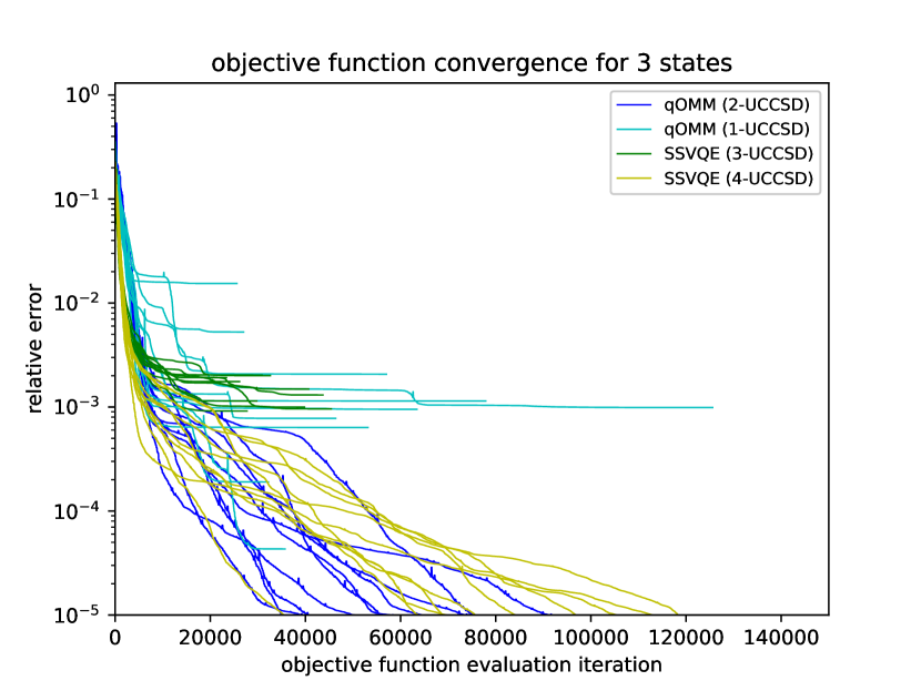
(b) Three states

Figure 15: Convergence of the relative error $\frac{\absolutevalue{f_{i}-f_{exact}}}{\absolutevalue{f_{exact}}}$ of qOMM and SSVQE for the hydrogen square model at an interatomic distance of 2.46 Å using a random parameter initialization.

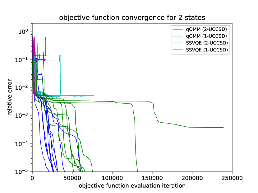
(a) Two states

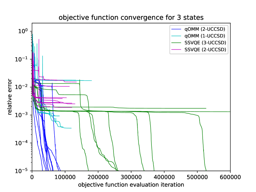
(b) Three states

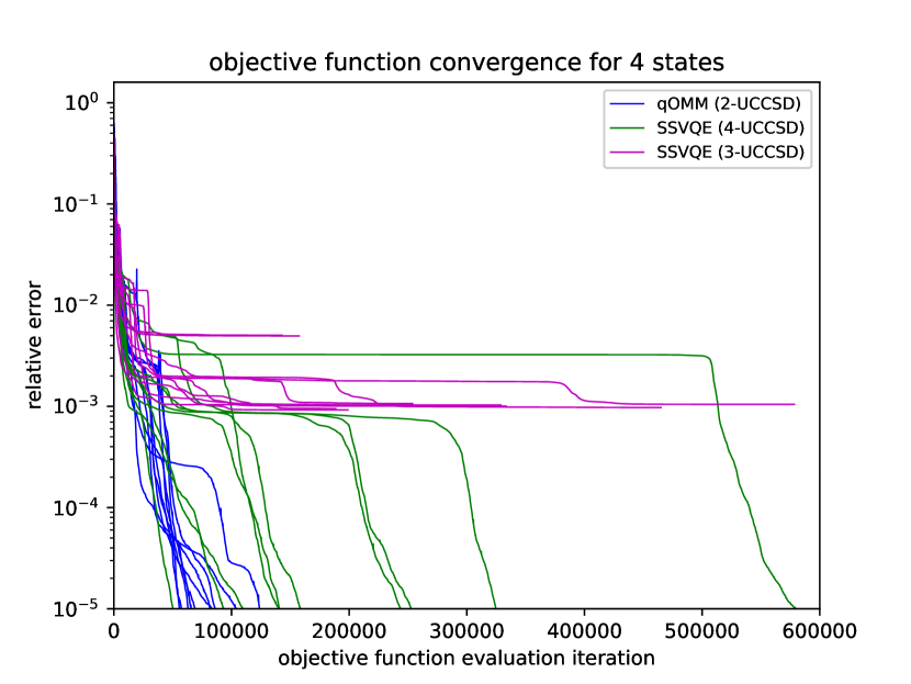
(c) Four states

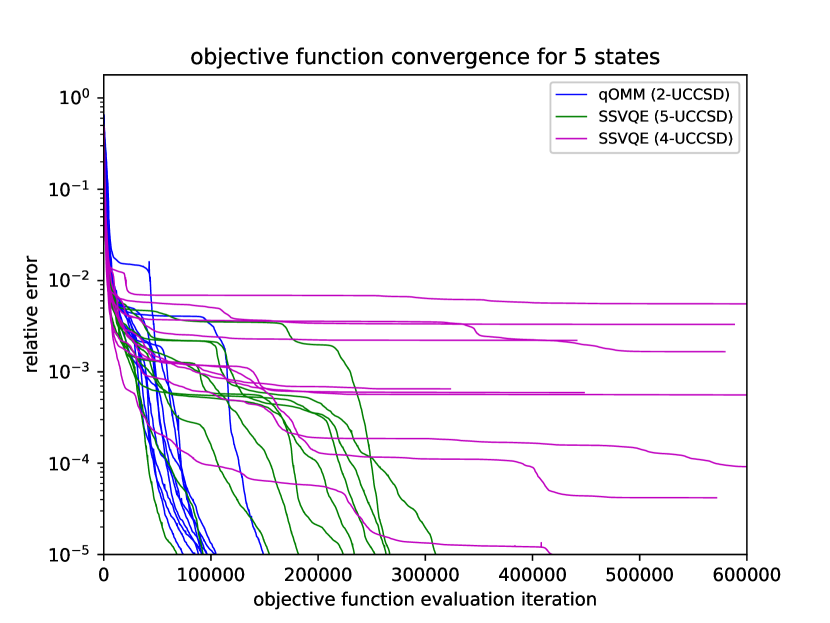
(d) Five states

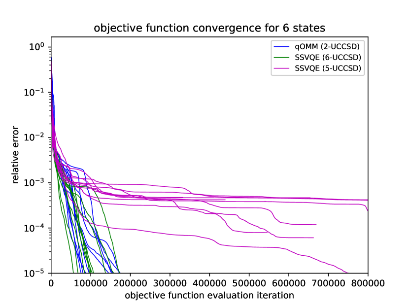
(e) Six states

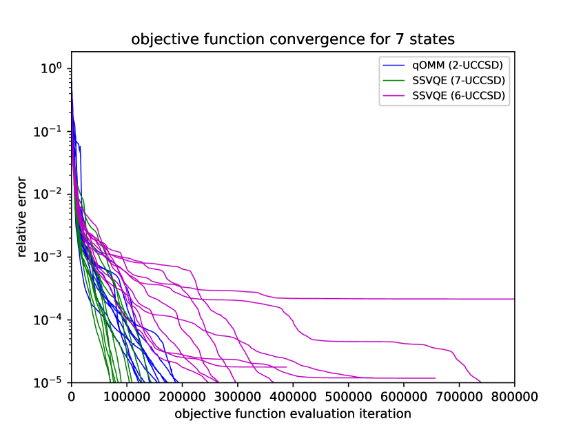
(f) Seven states

Figure 16: Convergence of the relative error $\frac{\absolutevalue{f_{i}-f_{exact}}}{\absolutevalue{f_{exact}}}$ of qOMM and SSVQE for LiH using randomly initialized parameters.

References

- Arute et al. 2019 Arute, F.; Arya, K.; Babbush, R.; Bacon, D. et al. Quantum supremacy using a programmable superconducting processor. Nature 2019 574:7779 2019, 574, 505–510
- Zhong et al. 2020 Zhong, H.-S.; Wang, H.; Deng, Y.-H.; Chen, M.-C. et al. Quantum computational advantage using photons. Science 2020, 370, 1460–1463
- Blunt et al. 2015 Blunt, N. S.; Smart, S. D.; Booth, G. H.; Alavi, A. An excited-state approach within full configuration interaction quantum Monte Carlo. J. Chem. Phys. 2015, 143, 134117
- Holmes et al. 2017 Holmes, A. A.; Umrigar, C. J.; Sharma, S. Excited states using semistochastic heat-bath configuration interaction. J. Chem. Phys. 2017, 147, 164111
- Schriber and Evangelista 2017 Schriber, J. B.; Evangelista, F. A. Adaptive configuration interaction for computing challenging electronic excited states with tunable accuracy. J. Chem. Theory Comput. 2017, 13, 5354–5366
- Li et al. 2019 Li, Y.; Lu, J.; Wang, Z. CoordinateWise descent methods for leading eigenvalue problem. SIAM J. Sci. Comput. 2019, 41, A2681–A2716
- Wang et al. 2019 Wang, Z.; Li, Y.; Lu, J. Coordinate descent full configuration interaction. J. Chem. Theory Comput. 2019, 15, 3558–3569
- Li and Lu 2020 Li, Y.; Lu, J. Optimal orbital selection for full configuration interaction (OptOrbFCI): Pursuing basis set limit under budget. J. Chem. Theory Comput. 2020, 16, 6207–6221
- Abrams and Lloyd 1999 Abrams, D. S.; Lloyd, S. Quantum algorithm providing exponential speed increase for finding eigenvalues and eigenvectors. Physical Review Letters 1999, 83, 5162–5165
- Aspuru-Guzik et al. 2005 Aspuru-Guzik, A.; Dutoi, A. D.; Love, P. J.; Head-Gordon, M. Simulated quantum computation of molecular energies. Science 2005, 309, 1704–1707
- Peruzzo et al. 2014 Peruzzo, A.; McClean, J.; Shadbolt, P.; Yung, M. H. et al. A variational eigenvalue solver on a photonic quantum processor. Nature Communications 2014, 5, 1–7
- Bauer et al. 2020 Bauer, B.; Bravyi, S.; Motta, M.; Chan, G. K.-L. Quantum algorithms for quantum chemistry and quantum materials science. Chemical Reviews 2020, 120, 12685–12717
- McArdle et al. 2020 McArdle, S.; Endo, S.; Aspuru-Guzik, A.; Benjamin, S. C. et al. Quantum computational chemistry. Reviews of Modern Physics 2020, 92, 015003
- McClean et al. 2017 McClean, J. R.; Kimchi-Schwartz, M. E.; Carter, J.; De Jong, W. A. Hybrid quantum-classical hierarchy for mitigation of decoherence and determination of excited states. Phys. Rev. A 2017, 95, 042308
- Colless et al. 2018 Colless, J. I.; Ramasesh, V. V.; Dahlen, D.; Blok, M. S. et al. Computation of molecular spectra on a quantum processor with an error-resilient algorithm. Physical Review X 2018, 8, 011021
- Ganzhorn et al. 2019 Ganzhorn, M.; Egger, D. J.; Barkoutsos, P.; Ollitrault, P. et al. Gate-efficient simulation of molecular eigenstates on a quantum computer. Physical Review Applied 2019, 11, 044092
- Ollitrault et al. 2020 Ollitrault, P. J.; Kandala, A.; Chen, C.-F.; Barkoutsos, P. K. et al. Quantum equation of motion for computing molecular excitation energies on a noisy quantum processor. Phys. Rev. Res. 2020, 2, 043140
- McClean et al. 2016 McClean, J. R.; Romero, J.; Babbush, R.; Aspuru-Guzik, A. The theory of variational hybrid quantum-classical algorithms. New J. Phys. 2016, 18, 23023
- Santagati et al. 2017 Santagati, R.; Wang, J.; Gentile, A. A.; Paesani, S. et al. Finding excited states of physical Hamiltonians on a silicon quantum photonic device. Front. Opt. 2017. 2017; p FM4E.2
- Santagati et al. 2018 Santagati, R.; Wang, J.; Gentile, A. A.; Paesani, S. et al. Witnessing eigenstates for quantum simulation of Hamiltonian spectra. Sci. Adv. 2018, 4, eaap9646
- Higgott et al. 2019 Higgott, O.; Wang, D.; Brierley, S. Variational quantum computation of excited states. Quantum 2019, 3, 156
- Jones et al. 2019 Jones, T.; Endo, S.; McArdle, S.; Yuan, X. et al. Variational quantum algorithms for discovering Hamiltonian spectra. Phys. Rev. A 2019, 99, 62304
- Nakanishi et al. 2019 Nakanishi, K. M.; Mitarai, K.; Fujii, K. Subspace-search variational quantum eigensolver for excited states. Physical Review Research 2019, 1, 033062
- Parrish et al. 2019 Parrish, R. M.; Hohenstein, E. G.; McMahon, P. L.; Martínez, T. J. Quantum computation of electronic transitions using a variational quantum eigensolver. Physical Review Letters 2019, 122, 230401
- Ordejon et al. 1993 Ordejon, P.; Drabold, D. A.; Grumbach, M. P.; Martin, R. M. Unconstrained minimization approach for electronic computations that scales linearly with system size. Physical Review B 1993, 48, 14646
- Mauri et al. 1993 Mauri, F.; Galli, G.; Car, R. Orbital formulation for electronic-structure calculations with linear system-size scaling. Physical Review B 1993, 47, 9973
- Lu and Thicke 2017 Lu, J.; Thicke, K. Orbital minimization method with regularization. J. Comput. Phys. 2017, 336, 87–103
- Byrd et al. 1995 Byrd, R. H.; Lu, P.; Nocedal, J.; Zhu, C. A Limited Memory Algorithm for Bound Constrained Optimization. SIAM Journal on Scientific Computing 1995, 16, 1190–1208
- Kandala et al. 2017 Kandala, A.; Mezzacapo, A.; Temme, K.; Takita, M. et al. Hardware-efficient variational quantum eigensolver for small molecules and quantum magnets. Nature 2017, 549, 242–246
- Gacon et al. 2021 Gacon, J.; Zoufal, C.; Carleo, G.; Woerner, S. Simultaneous perturbation stochastic approximation of the quantum Fisher information. Quantum 2021, 5, 567
- Childs and Wiebe 2012 Childs, A. M.; Wiebe, N. Hamiltonian simulation using linear combinations of unitary operations. Quantum Info. Comput. 2012, 12, 901–924
- Romero et al. 2018 Romero, J.; Babbush, R.; McClean, J. R.; Hempel, C. et al. Strategies for quantum computing molecular energies using the unitary coupled cluster ansatz. Quantum Science and Technology 2018, 4, 014008
- ANIS et al. 2021 ANIS, M. S.; Abraham, H.; AduOffei,; Agarwal, R. et al. Qiskit: An Open-source Framework for Quantum Computing. 2021
- Sun et al. 2018 Sun, Q.; Berkelbach, T. C.; Blunt, N. S.; Booth, G. H. et al. PySCF: the python-based simulations of chemistry framework. Wiley Interdisciplinary Reviews: Computational Molecular Science 2018, 8, e1340
- Bravyi et al. 2017 Bravyi, S.; Gambetta, J. M.; Mezzacapo, A.; Temme, K. Tapering off qubits to simulate fermionic Hamiltonians. 2017; \urlhttps://arxiv.org/abs/1701.08213
- Gao et al. 2020 Gao, W.; Li, Y.; Lu, B. Triangularized orthogonalization-free method for solving extreme eigenvalue problems. 2020; \urlhttp://arxiv.org/abs/2005.12161
- Gao et al. 2021 Gao, W.; Li, Y.; Lu, B. Global Convergence of Triangularized Orthogonalization-free Method. 2021; https://arxiv.org/abs/2110.06212v1
- Allen-Zhu et al. 2019 Allen-Zhu, Z.; Li, Y.; Liang, Y. Learning and generalization in overparameterized neural networks, going beyond two layers. Advances in Neural Information Processing Systems. 2019
- Cincio et al. 2018 Cincio, L.; Subaşı, Y.; Sornborger, A. T.; Coles, P. J. Learning the quantum algorithm for state overlap. New Journal of Physics 2018, 20, 113022
- Cerezo et al. 2021 Cerezo, M.; Sone, A.; Volkoff, T.; Cincio, L. et al. Cost function dependent barren plateaus in shallow parametrized quantum circuits. Nature Communications 2021, 12, 1791
- Wang et al. 2021 Wang, S.; Fontana, E.; Cerezo, M.; Sharma, K. et al. Noise-induced barren plateaus in variational quantum algorithms. Nature Communications 2021, 12, 6961
- Li and Lu 2020 Li, Y.; Lu, J. Optimal Orbital Selection for Full Configuration Interaction (OptOrbFCI): Pursuing the Basis Set Limit under a Budget. Journal of Chemical Theory and Computation 2020, 16, 6207–6221, PMID: 32786901
- Grimsley et al. 2019 Grimsley, H. R.; Economou, S. E.; Barnes, E.; Mayhall, N. J. An adaptive variational algorithm for exact molecular simulations on a quantum computer. Nature Communications 2019, 10, 1–9
- Tang et al. 2021 Tang, H. L.; Shkolnikov, V.; Barron, G. S.; Grimsley, H. R. et al. Qubit-ADAPT-VQE: An adaptive algorithm for constructing hardware-efficient ansätze on a quantum processor. PRX Quantum 2021, 2, 020310
- Yordanov et al. 2021 Yordanov, Y. S.; Armaos, V.; Barnes, C. H.; Arvidsson-Shukur, D. R. Qubit-excitation-based adaptive variational quantum eigensolver. Communications Physics 2021, 4, 1–11