Nebular-Phase Spectra of Type Ia Supernovae from the Las Cumbres Observatory Global Supernova Project

Abstract

The observed diversity in Type Ia supernovae (SNe Ia) – the thermonuclear explosions of carbon-oxygen white dwarf stars used as cosmological standard candles – is currently met with a variety of explosion models and progenitor scenarios. To help improve our understanding of whether and how often different models contribute to the occurrence of SNe Ia and their assorted properties, we present a comprehensive analysis of seven nearby SNe Ia. We obtained one to two epochs of optical spectra with Gemini Observatory during the nebular phase ($>$200 days past peak) for each of these events, all of which had time-series of photometry and spectroscopy at early times (the first $\sim$8 weeks after explosion). We use the combination of early- and late-time observations to assess the predictions of various models for the explosion (e.g., double-detonation, off-center detonation, stellar collisions), progenitor star (e.g., ejecta mass, metallicity), and binary companion (e.g., another white dwarf or a non-degenerate star). Overall, we find general consistency in our observations with spherically-symmetric models for SN Ia explosions, and with scenarios in which the binary companion is another degenerate star. We also present an in-depth analysis of SN 2017fzw, a member of the sub-group of SNe Ia which appear to be transitional between the subluminous “91bg-like" events and normal SNe Ia, and for which nebular-phase spectra are rare.

1 Introduction

Type Ia supernovae (SNe Ia) are well-established to be the thermonuclear explosions of carbon-oxygen white dwarf stars (e.g., Hillebrandt & Niemeyer, 2000; Maoz et al., 2014). The detonation synthesizes radioactive ⁵⁶Ni, which decays to ⁵⁶Co and then ⁵⁶Fe, powering the light curve. The mass of synthesized ⁵⁶Ni is known to be the primary physical cause of the light-curve width-luminosity correlation which allows SNe Ia to be used as cosmological standard candles (e.g., Pskovskii, 1977; Phillips, 1993). During the photospheric phase in the months after explosion, while the ejecta material is still optically thick, SN Ia spectra are dominated by high-velocity absorption features of Si ii, S ii, Mg ii, and Ca ii. However, at $>$200 days after peak brightness, the ejecta material becomes optically thin and the optical spectra are dominated by forbidden emission lines from the nucleosynthetic products: iron, cobalt, and nickel. The velocity, width, and flux in these lines can reveal the amount and spatial distribution of these elements within the nebula. Correlations between late- and early-time observations are particularly useful to understand some of the open questions regarding the progenitor white dwarf, the explosion mechanism, and the binary companion star type.

Explosion Mechanism – Some of the open questions regarding SN Ia explosions include whether the detonation is preceded by a deflagration phase of slow burning in the core (the “delayed detonation" model) and how long that phase might be (e.g., Khokhlov, 1991; Arnett & Livne, 1994; Seitenzahl et al., 2013); whether and how a surface detonation of accrued material can initiate a core detonation (the “double detonation" model; Wiggins et al. 1998; Fink et al. 2007); whether and how often a detonation can be instigated by a violent merger with a binary companion star (e.g., Pakmor et al., 2011; Kromer et al., 2016); and whether and how the white dwarf’s mass affects the explosion and the observed SN Ia properties, especially when it is less than the Chandrasekhar mass of 1.4 $\rm M_{\odot}$ (e.g., Blondin et al., 2017; Polin et al., 2019). For example, the fact that nickel is seen in late-time spectra indicates that the density of the progenitor white dwarf was high enough to burn to stable nickel (as the radioactive ⁵⁶Ni has decayed by the nebular phase), and this density requirement has traditionally excluded white dwarfs that are substantially below the Chandrasekhar mass (Wilk et al., 2018). However, recent simulations by Shen et al. (2021) have shown for the first time that white dwarf explosions for a wide range of masses, including sub-Chandrasekhar mass, can reproduce the observed characteristics of normal SNe Ia. Furthermore, many explosion models predict different spatial/velocity distributions for the nucleosynthetic material, and/or different mass ratios for stable and radioactive materials, which can be investigated with nebular-phase spectra.

Explosion Asymmetry – Maeda et al. (2010a) present a model for asymmetric explosions in which SNe Ia with a detonation that is offset “away" from the observer results in both a red-shifted nebular feature and a quickly-declining velocity for the Si ii $\lambda$6355 Å absorption feature in the two weeks after peak brightness (a “high velocity gradient", HVG; Benetti et al. 2005), and vice versa for offsets “towards" the observer (a blue-shifted nebular feature and a low velocity gradient, LVG). So far, SN Ia observations show that most HVG SNe Ia exhibit red-shifted nebular features, but it remains unclear whether explosion asymmetry is the unique explanation for this trend. Another source of asymmetry in SN Ia explosions could be head-on collisions between white dwarf stars (WD-WD collisions), potentially driven into highly elliptical orbits by a tertiary star (e.g., Rosswog et al., 2009; Raskin et al., 2009; Kushnir et al., 2013). If such a collision was aligned with the observer’s line-of-sight, the velocities of the WD-WD pair could cause double-peaked nebular-phase emission features (e.g., Dong et al., 2015). However, Wang et al. (2013) argued that the observed diversity in SNe Ia might be due to progenitor environment (i.e., progenitor metallicity), instead of explosion asymmetry.

Progenitor Metallicity – Timmes et al. (2003) describe how the additional neutrons available in higher-metallicity white dwarf stars might lead to a higher ratio of stable-to-radioactive nucleosynthetic products. At early times, higher-metallicity progenitors might exhibit a depressed near-ultraviolet (NUV) flux due to line blanketing (Lentz et al., 2000). In the nebular phase, higher metallicity could manifest as a higher Ni/Fe ratio, as all the radioactive ⁵⁶Ni would have decayed, leaving stable nickel as the source of forbidden emission line [Ni ii] $\lambda$7378 Å.

Non-degenerate Companions – Whether and how often the binary companion star is another white dwarf (the double-degenerate scenario), or a main sequence or red giant star (the single-degenerate scenario), is not yet well constrained. The presence of a main sequence or red giant companion star could be revealed by a “blue bump" in the very early-time light curve (within a few days of explosion; Kasen 2010), and/or by a narrow H$\alpha$ emission feature from hydrogen swept off of a non-degenerate companion and embedded in the expanding nebula (e.g., Mattila et al., 2005; Leonard, 2007). So far, no SN Ia has exhibited both potential signatures of a non-degenerate companion star.

In this work, we present nebular-phase optical and infrared spectroscopy from Gemini Observatory for seven nearby SNe Ia with early-time (first $\lesssim$2 months after explosion) optical photometry and spectroscopy from the Las Cumbres Observatory (Brown et al., 2013) and, in most cases, from other facilities as well. We describe the targeted sample of SNe Ia and present relevant early-time data in Section 2, and present and analyze our nebular-phase observations – and measure parameters for the forbidden emission lines of nickel, cobalt, and iron – in Section 3. In Section 4 we analyze our sample of nebular-phase spectra as a whole, and compare with previously published samples, in order to assess general physical models for SN Ia explosions and progenitor scenarios. In Section 5 we provide unique in-depth physical analyses based on the early- and late-time data for each individual SN Ia. A summary of our conclusions is provided in Section 6. In this work we assume a flat cosmology of $H_{0}=70$ $\rm km\ s^{-1}\ Mpc^{-1}$, $\Omega_{M}=0.3$, and $\Omega_{\Lambda}=0.7$, and quote all light curve phases in days from peak brightness unless otherwise specified.

2 The Sample of Nearby SNe Ia

The Las Cumbres Observatory’s (Brown et al., 2013) Global Supernova Project (GSP) obtains optical photometry and spectroscopy of nearby SNe with a regular cadence. The GSP engages in this monitoring to enable studies of both large samples of SNe and of rare events, such as SNe that are very nearby or peculiar in some way. From the GSP-monitored sample we selected SNe Ia for nebular-phase spectroscopy at Gemini Observatory that were well offset from their host galaxy (Figure 1), were nearby enough to be $B\lesssim 22$ mag at $>$200 days after peak brightness, had a well-sampled early-time light curve through $\sim$30 days post-peak (so that the phase and brightness at maximum can be measured), and had at least 2 spectral epochs in the $\sim$2 weeks after peak brightness (so that the photospheric velocity and its gradient can be measured). After applying those criteria, we prioritized SNe Ia which were otherwise peculiar, such as those that showed deviations in their early-time light curve or belonged to sub-classes such as SN 1991bg-like (Filippenko et al., 1992).

In Table 1 we list the names and coordinates of the SNe Ia included in this analysis, along with their redshift and distance derived from their host galaxy properties, and the line-of-sight Galactic extinction for their coordinates. In Table 2 we list the early-time qualities of our sample’s light curves and spectra, based either on data from the Las Cumbres Observatory or other published works as cited in Table 2 and as described in Sections 2.1 and 2.2. These early-time qualities are incorporated into the analysis and discussion of these individual SNe Ia in Section 5.

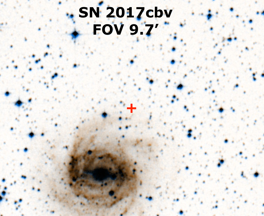
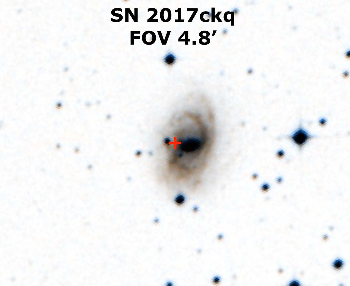
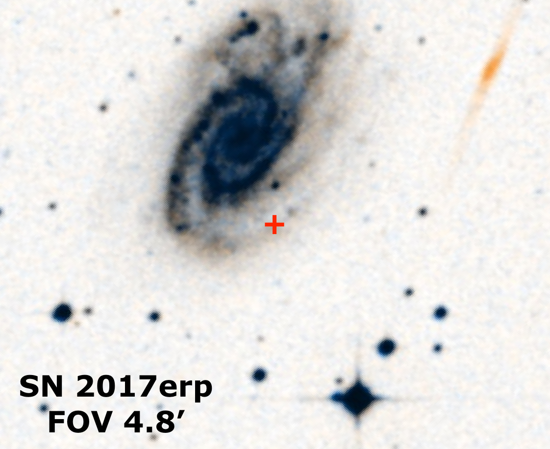
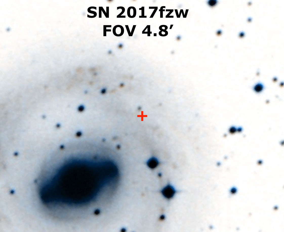
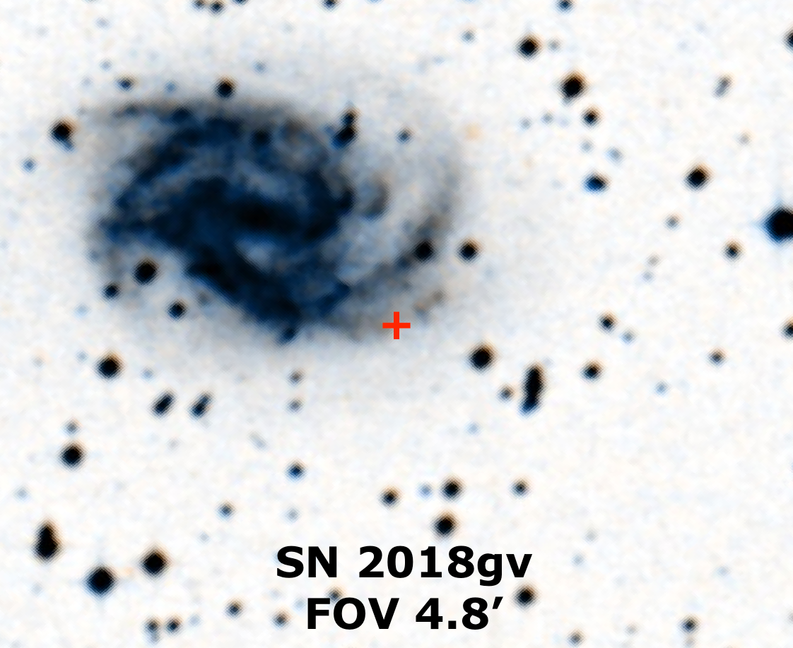
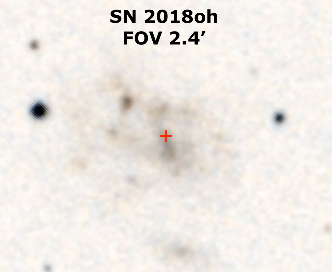
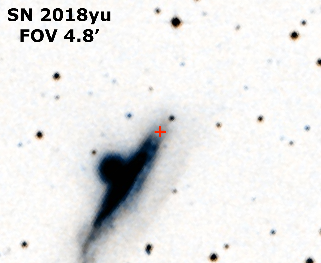
Figure 1: Image stamps from the Digital Sky Survey (inverse color), centered on the location of each of our SN Ia (red cross), to illustrate the location of each with respect to its host galaxy. All images are north-up east-left, and have fields of view (FOV) as indicated.

SN Name	Coordinates	Redshift	Distance	Galactic Extinction[1]
	RA,Dec (J2000)	($z$)	(Mpc)	$A_{B}$ (mag)	$E(B-V)$ mag
2017cbv	14:32:34.38, -44:08:03.1	0.00399[2]	$16.9\pm 3.1^{\rm[3]}$	0.5956	0.1452
2017ckq	10:44:25.39, -32:12:32.8	$0.0100\pm 0.0001^{\rm[4]}$	42.9[5]	0.2657	0.0648
2017erp	15:09:14.81, -11:20:03.2	$0.006174\pm 0.000003^{\rm[6]}$	$29.4\pm 1.3^{\rm[7]}$	0.3800	0.0928
2017fzw	06:21:34.77, -27:12:53.5	0.0054[2]	19.5[3]	0.1512	0.0369
2018gv	08:05:34.61, -11:26:16.3	0.0053[2]	16.8[5]	0.2040	0.0497
2018oh	09:06:39.59, +19:20:17.5	0.010981[9]	$47.9\pm 1.9$ [7]	0.1552	0.0368
2018yu	05:22:32.36, -11:29:13.8	0.00811[2]	37.1[8]	0.5363	0.1306

Table 1: A list of the SNe Ia included in this study. [1] Extinction values are from Schlafly & Finkbeiner (2011), and assume Galactic $R_{V}=3.1$. [2] de Vaucouleurs et al. (1991). [3] Tully (1988). [4] Mould et al. (2000). [5] Tully et al. (2013). [6] Theureau et al. (2005). [7] Könyves-Tóth et al. (2020). [8] Theureau et al. (2007). [9] Schneider et al. (1990).

		Early-Time $B$-Band Light Curve			Early-Time Photospheric Si ii
SN Ia	Sub-	Peak Date	Peak Brightness	Decline Rate	Velocity[1]	Gradient[2]	Class[3]
Name	Type	(in $B$; UT)	($B$-band mag)	$\Delta m_{\rm 15}(B)$ (mag)	($\rm km\ s^{-1}$)	($\rm km\ s^{-1}\ d^{-1}$)
2017cbv	99aa	2017-03-29.1[4]	-19.25[5]	1.06[4]	$-9300\pm 60$	$19\pm 8$	LVG
2017ckq		2017-04-08.1	$-18.9\pm 0.3$	$0.96\pm 0.20$	$-10500\pm 200$	$71\pm 23$	$\sim$HVG
2017erp		2017-06-30.9[6]	$-19.50\pm 0.15^{\rm[6,7]}$	$1.129\pm 0.011^{\rm[7]}$	$-10500\pm 100$	$78\pm 13$	$\sim$HVG
2017fzw	91bg/trans	2017-08-22.9[8]	$-18.81\pm 0.18^{\rm[8]}$	$1.60\pm 0.02^{\rm[8]}$	$-13800\pm 400$	$300\pm 50$	FAINT
2018gv		2018-01-31[9]	$-19.1^{\rm[9]}$	$0.96^{\rm[9]}$	$-11100\pm 90$	$29\pm 4$	LVG
2018oh		2018-02-13.7[10]	$-19.47\pm 0.10^{\rm[10]}$	$0.96\pm 0.03^{\rm[10]}$	$-10100\pm 10$	$69\pm 4^{\rm[10]}$	LVG
2018yu		2018-03-17.9	$-19.1\pm 0.5$	$1.05\pm 0.05$	$-9500\pm 120$	$45\pm 21$	LVG

Table 2: The characteristic quantities from the early-time data for our targeted SNe Ia. All values derived in this work unless otherwise cited. [1] Si ii velocity at peak brightness. [2] Rate of decline of Si ii during the first two weeks after peak brightness. [3] Low (L) or high (H) velocity gradient (VG) group (division at $70$ $\rm km\ s^{-1}\ day^{-1}$) or the FAINT group (Benetti et al., 2005). [4] Hosseinzadeh et al. (2017a). [5] Sand et al. (2018a). [6] Brown et al. (2019). [7] Könyves-Tóth et al. (2020). [8] Galbany et al., (in prep.) . [9] Yang et al. (2020). [10] Li et al. (2019).

2.1 Near-Peak Optical Photometry

MJ Date	$B$ Mag	$V$ Mag
SN 2017ckq:
57844.1	$14.58\pm 0.25$	$14.51\pm 0.27$
57848.7	$14.27\pm 0.15$	$14.28\pm 0.20$
57851.9	$14.29\pm 0.17$	$14.24\pm 0.21$
57853.6	$14.26\pm 0.09$	$13.97\pm 0.09$
57857.6	$14.55\pm 0.09$	$14.34\pm 0.11$
57861.8	$14.70\pm 0.30$	$14.44\pm 0.19$
57866.2	$15.26\pm 0.26$	$14.76\pm 0.25$
57870.2	$15.71\pm 0.38$	$14.96\pm 0.26$
SN 2018yu:
58186.0	$14.66\pm 0.09$	$14.54\pm 0.08$
58189.0	$14.25\pm 0.05$	$14.12\pm 0.06$
58192.0	$14.06\pm 0.07$	$13.91\pm 0.06$
58193.1	$14.02\pm 0.05$	$14.03\pm 0.04$
58195.0	$14.02\pm 0.07$	$13.87\pm 0.06$
58196.0	$14.03\pm 0.05$	$13.87\pm 0.06$
58197.0	$14.06\pm 0.05$	$13.88\pm 0.06$
58201.4	$14.26\pm 0.08$	$14.06\pm 0.06$
58205.0	$14.51\pm 0.05$	$14.22\pm 0.06$
58211.1	$15.20\pm 0.07$	$14.56\pm 0.06$

Table 3: The near-peak $B$- and $V$-band photometry from Las Cumbres Observatory used to measure the light curve properties of SNe Ia 2017ckq and 2018yu. For all of our other targets, the light curve parameters that we use are from previously published work.

The existence of near-peak optical photometry from the Las Cumbres Observatory was one of the selection criteria for the SNe that we targeted for nebular-phase spectroscopy with Gemini Observatory. However, since most of our targets were interesting nearby events, by the time of this nebular-phase analysis five of our seven targets already had publications based on analyses of early-time photometry. These publications included the derived light curve parameters of peak date, peak brightness, and decline rate in the $B$ filter which are needed for contextual analysis of our nebular-phase spectra. Instead of recalculating these properties based on Las Cumbres photometry, for these five SNe Ia we have adopted the published values and cited the appropriate literature in Table 2. For the two SNe Ia which did not have published light curve parameters, SNe 2017ckq and 2018yu, we provide their near-peak $B$- and $V$-band photometry from the Las Cumbres Observatory in Table 3, and discuss their light curves below.

SN 2017ckq – Photometric monitoring with the Las Cumbres Observatory shows that SN 2017ckq peaked in $B$-band brightness on 2017-04-08.1 UT at $14.3\pm 0.1$ mag and exhibited a decline rate of $\Delta m_{\rm 15}(B)\approx 0.96\pm 0.2$ mag. These measurements are based on a third-order polynomial fit to the host-subtracted SN photometry listed in Table 3. The underlying host galaxy surface brightness at the location of SN 2017ckq is quite faint, $\mu_{B}\approx 22.6$ $\rm mag\ arcsec^{-2}$ (despite the impression given by the DSS image in Figure 1). Photometry was measured using Source Extractor (Bertin & Arnouts, 1996) and calibrated using the APASS star catalog (Henden et al., 2016). Based on the $V$-band observations near $B$-band peak brightness, the color $B-V$ is consistent with $0$, suggesting a low amount of host galaxy extinction. Given the host galaxy distance, the peak absolute magnitude of SN 2017ckq is $M_{B}\approx-18.9\pm 0.3$ mag.

SN 2018yu – Photometric monitoring with the Las Cumbres Observatory shows that SN 2018yu peaked in $B$-band brightness on 2018-03-17.9 UT at $14.02\pm 0.05$ mag and exhibited a decline rate of $\Delta m_{\rm 15}(B)\approx 1.05\pm 0.05$ mag. These measurements are based on a third-order polynomial fit to the host-subtracted SN photometry listed in Table 3. The underlying host galaxy surface brightness at the location of SN 2018yu is very faint, $\mu_{B}\approx 23.6$ $\rm mag\ arcsec^{-2}$. As with SN 2017ckq, photometry was measured using Source Extractor (Bertin & Arnouts, 1996) and calibrated using the APASS star catalog (Henden et al., 2016). At peak $B$-band brightness, the SN’s color is $B-V\approx 0.14$ mag, suggesting $\leq 0.2$ mag of extinction due to the host galaxy. We correspondingly adjust the peak apparent brightness to be $B\approx 13.8\pm 0.1$ mag. However, we also note that early-time optical spectra obtained by the Las Cumbres Observatory exhibit a host-galaxy component of Na iD at $z=0.01$ with an equivalent width of $\approx 0.3$ Å, and that this corresponds to an approximate host-galaxy $E(B-V)\approx 0.03$ based on the empirical relation derived in Poznanski et al. (2012), which suggests less host-galaxy extinction ($<0.1$ mag, assuming $R_{V}=3.1$). The peak absolute magnitude of SN 2018yu is $M_{B}\approx-19.1\pm 0.5$ mag, with most of that uncertainty due to the host galaxy’s distance error.

2.2 Photospheric Velocity Classifications

SN Name	Date	SN Name	Date
2017cbv	2017-03-31	SN2017fzw	2017-08-13
	2017-04-03		2017-09-02
	2017-04-07		2017-09-07
	2017-04-07		2017-09-14
	2017-04-13	SN2018gv	2018-02-04
SN2017ckq	2017-04-09		2018-02-08
	2017-04-13		2018-02-13
	2017-04-17	SN2018oh	2018-02-14
	2017-04-21		2018-02-20
SN2017erp	2017-06-30	SN2018yu	2018-03-16
	2017-07-06		2018-03-19
	2017-07-12		2018-03-20
	2017-07-15		2018-03-24
			2018-03-28

Table 4: The early-time spectra from FLOYDS at Las Cumbres that were used to determine the Si ii velocity gradients.

We use early-time optical spectroscopy from the FLOYDS robotic spectrograph on the Las Cumbres Observatory 2 meter telescopes, as listed in Table 4, to measure each SN’s photospheric velocity and velocity gradient, and to classify each SN as belonging to the low- or high-velocity gradient sub-classes (LVG/HVG Benetti et al., 2005). To measure the photospheric velocity, we smooth the FLOYDS optical spectra with a Savitsky-Golay filter of width $\sim 20$–$50$ Å, use the minimum of the Si ii $\lambda$ 6355 Å line as representative of the velocity of the photosphere, and bootstrap (shuffle the flux uncertainties between pixels, simulate a new observed flux values, and remeasure the line velocity) to estimate the uncertainty in the velocity measurement. We measure the photospheric velocity in this way for all spectra obtained by the Las Cumbres Observatory between phases of $0$ to $15$ days after peak brightness, and then do a linear regression to interpolate the velocity at peak ($v_{\rm SiII}$) and to estimate velocity gradient ($\dot{v}_{\rm SiII}$), which are quoted in columns 6 and 7 of Table 2. Several modifications made to this technique for a few of our SNe Ia, as discussed in the paragraphs below. In column 8 of Table 2 we assign each SN Ia to either the low- and high-velocity gradient groups (L/HVG) based on whether their $\dot{v}_{\rm SiII}$ is below or above $70$ $\rm km\ s^{-1}\ day^{-1}$, as defined by Benetti et al. (2005). For SNe Ia which have an uncertainty that overlaps the boundary we represent this uncertainty by assigning the type as $\sim$L/HVG.

SN 2017erp – Our measured velocity gradient for SN 2017erp of $\dot{v}_{\rm SiII}=78\pm 13$ $\rm km\ s^{-1}\ day^{-1}$ was obtained from FLOYDS spectra at $-0.8$, $5$, and $11$, and $14$ days (Table 4), combined with two spectra from Lick Observatory which were obtained at phases of $0.1$ and $4$ days (Stahl et al., 2020). This velocity gradient is greater than the $70$ $\rm km\ s^{-1}\ day^{-1}$ minimum for classifying a SN Ia as “high velocity gradient" (HVG), but since the error bar does overlap with that cutoff, we list SN 2017erp as “$\sim$HVG" in Table 2. Our measured photospheric velocity for SN 2017erp of $v_{\rm SiII}=-10500\pm 100$ $\rm km\ s^{-1}$ is an average of the velocities from the $-0.8$ and $0.1$ day spectra.

SN 2017fzw – Our estimate for the photospheric velocity is a special case because 91bg-like and transitional events evolve quickly, but our spectral sampling is relatively sparse – the four near-peak spectral epochs are at phases $-12$, $8$, $13$, and $20$ days – and there are no supplemental publicly-available near-peak optical spectra for this object. We fit a line between the first two epochs in order to estimate the velocity at peak brightness, and between the second two epochs to estimate the velocity gradient, and bootstrap our uncertainty estimates based on line fits with two, three, and all four epochs. Since the low- and high-velocity gradient groups apply to normal SNe Ia, we do not assign an L/HVG subclass for SN 2017fzw in Table 2, and instead label it as FAINT to be consistent with Benetti et al. (2005).

SN 2018oh – The peak velocity is taken directly from a FLOYDS spectrum with a phase of $0$ days. There is only one other FLOYDS spectrum within the first two weeks after peak brightness, at $6$ days, and both spectra are relatively noisy. We find that the application of a Monte Carlo analysis to estimate the slope between these two points finds a velocity gradient of $75\pm 65$ $\rm km\ s^{-1}\ day^{-1}$. This is an insufficient confidence to declare SN 2018oh a member of the HVG subgroup, especially since its velocity at peak brightness is low. Instead, we use the work of Li et al. (2019), who present a dense time-series of optical spectroscopy which exhibit a photospheric Si ii velocity at peak brightness of $10300$ $\rm km\ s^{-1}$, and a velocity gradient over the first 10 days after peak brightness of $69\pm 4$ $\rm km\ s^{-1}\ day^{-1}$, which is on the high side but puts SN 2018oh in the LVG class.

3 Nebular-Phase Observations

We obtained spectroscopic observations of the seven SNe Ia in our sample at $>200$ days after peak brightness primarily via a targeted follow-up program at Gemini Observatory, but also used late-time observations from other facilities. This section describes the acquisition, reduction, and calibration of these spectra, and measurements of nebular-phase emission line parameters such as velocity, full-width at half-max (FWHM), and integrated flux.

3.1 Optical Spectra from Gemini Observatory

The observation dates, instrument configurations, and exposure times for the longslit optical spectroscopy of the SNe Ia in our sample that we obtained with Gemini Observatory’s Gemini Multi-Object Spectrograph (GMOS) in longslit mode (Hook et al., 2004) are listed in Table 6 in Appendix A. To reduce and calibrate our data, internal spectroscopic flats and CuAr arc lamps were obtained during the night, before or after the object exposures, bias frames during the day, and standard stars were observed in the same configuration within a few nights. Data were reduced with IRAF using custom scripts based on the Gemini data reduction cookbook (Shaw, 2016). One-dimensional spectra were extracted from each reduced, sky-subtracted, two-dimensional spectrum, and adjacent pixels were used to fit for and remove as much contaminating flux from the host galaxy as possible (but some residuals remain; e.g., from emission lines with spatial variation at the SN’s location).

These extracted 1D spectra were corrected for atmospheric extinction and the instrumental sensitivity function, sigma-clipped to reject artifact pixels from, e.g., cosmic rays, and then median-combined. To create a single joined spectrum for each observational epoch, the R400 spectra were flux-matched to the B600 spectra and two were joined in the middle of the overlap region (${\sim}5500$ Å). The spectra were then flux-calibrated to the late-time photometry estimates listed in Table 5. These estimates were interpolated or extrapolated from imaging obtained within days to weeks of our nebular spectra, but very precise calibration is not necessary for our analysis and mainly used for display in Figure 2. After this approximate flux calibration, spectra were corrected for line-of-sight dust extinction using the astropy-affiliated dust_extinction package and the $E(B-V)$ parameters listed in Table 1, and corrected to rest-frame wavelengths using the redshifts listed in Table 1. Plots of all of our Gemini spectra are shown in Figure 2, with scaled spectra of the fiducial SN Ia 2011fe at similar phases for comparison.

SN Name	Phase	Photometry	Reference
	[days]	[mag]
2017cbv	466	V$\sim$20.8	[2]
2017ckq	369	G$\sim$21.7	Gaia17bhb [1]
2017erp	259	V$\sim$19.6	[2]
2017fzw	234	G$\sim$20.1	Gaia17cbe [1]
2018gv	289	G$\sim$19.6	Gaia18bat [1]
2018gv	344	G$\sim$20.5	Gaia18bat [1]
2018oh	264	G$\sim$20.6	Gaia18awj [1]
2018yu	202	V$\sim$19.3	[2]
2018yu	287	V$\sim$20.3	[2]

Table 5: Late-time photometric estimates for the SNe Ia in our sample. Epochs that were near in time to our spectroscopic observations were interpolated (or extrapolated) to estimate photometric measurements. [1] Gaia Alerts, Wyrzykowski et al. (2012). [2] Las Cumbres Observatory Global Supernova Project.

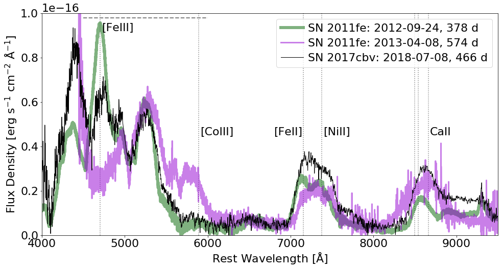
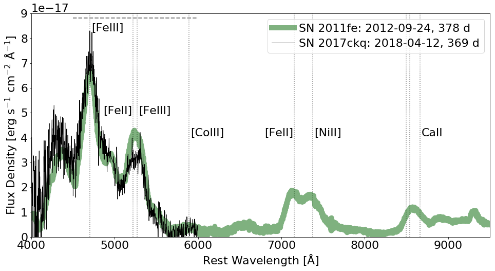
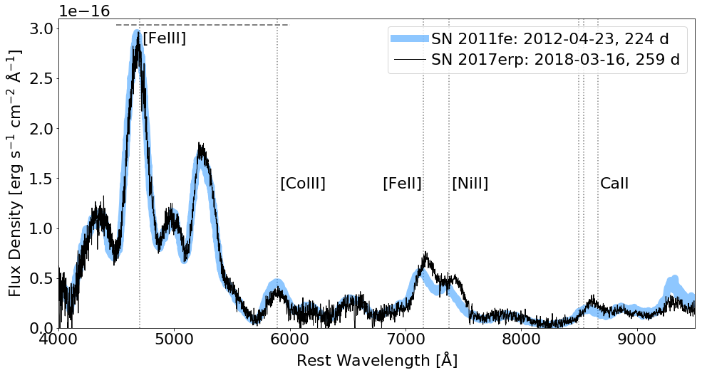
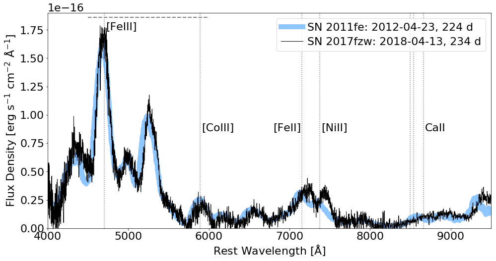
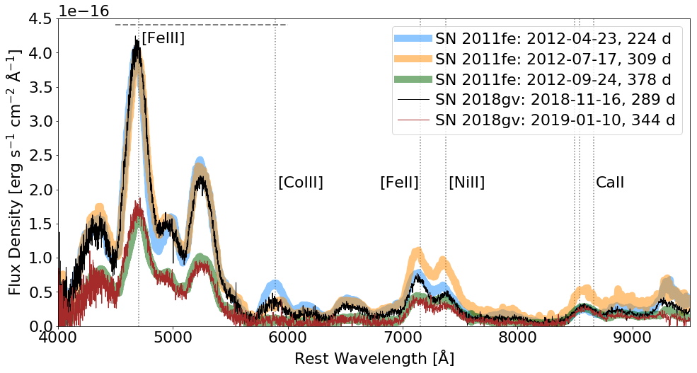
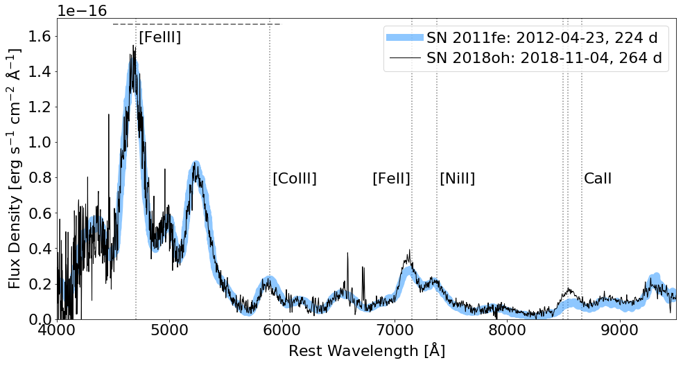
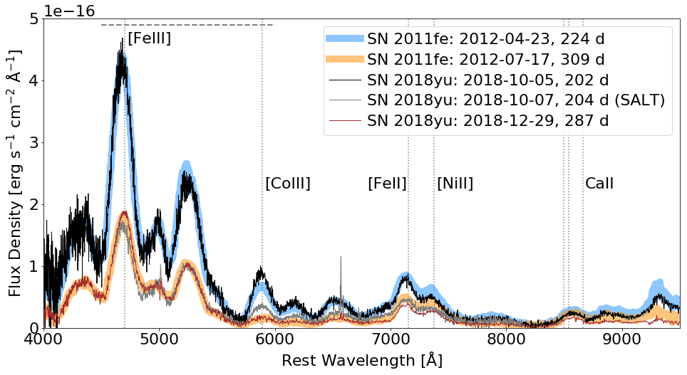
Figure 2: Comparisons of the nebular-phase optical spectra in our Gemini sample (thin black lines; brown for second epochs; grey for SALT) with spectra of SN 2011fe at a similar phase (thick semi-transparent colored lines). The 224 (blue) and 309 (orange) day spectra of SN 2011fe are from Graham et al. (2015a); the 378 (green) day from Stahl et al. (2020); and the 574 (violet) day from Graham et al. (2015b). Spectra of SN 2011fe have been scaled to match the integrated flux of our spectra from $\sim$4500 to $\sim$6000 Å (dashed horizontal line). The dominant species for some emission features of interest are labeled with dotted vertical lines.

3.2 Optical Spectra from the South African Large Telescope

One nebular-phase spectrum of SN 2018yu was obtained with the South African Large Telescope (SALT) Robert Stobie Spectrograph (RSS) using the 1.5″ longslit and the PG0900 grating (resolution $\sim 5.6$ Å). The grating’s central wavelength was shifted between six exposures to cover the full optical range $4600$ to $8200$ Å, using a filter to block second order contamination for red settings. The six exposures had a total exposure time of 2386 seconds. This spectrum was corrected for line-of-sight dust extinction (as described above), de-redshifted, and is co-plotted in Figure 2. Without any flux scaling, this SALT spectrum for SN 2018yu at $204$ days past peak appears to match the Gemini spectrum at $202$ days quite well.

3.3 Near-Infrared Spectroscopy from Gemini Observatory

A nebular phase near-infrared (NIR) spectrum of SN 2018yu at 282 days past maximum was obtained using the long slit mode of Flamingos-2 on Gemini South (Eikenberry et al., 2008). The spectrum was observed using the JH filter and grism with a 3 pixel slit centered at 1.39 $\mu$m. Using the standard ABBA nod-along-the-slit convention, we obtained a total of 104 exposures of 120 seconds each for SN 2018yu over the course of two consecutive nights. Standard star observations of a nearby A0V star were obtained immediately before and after the SN observations, as well as a flat and arc for wavelength calibrations. NIR spectra were reduced using Gemini IRAF and the Flamingos-2 Data Reduction Cookbook. The spectra were also corrected for the atmosphere’s telluric absorption using xtellcor and the method presented in Vacca et al. (2003). The final NIR spectrum of SN 2018yu, presented in Section 5.7, is a combination of observations obtained over two consecutive nights that was combined after each night’s observations were reduced, and telluric corrected separately using that night’s standard star observations and associated calibrations.

3.4 Nebular Emission Line Parameters

We use two methods, “direct measure" and “Gaussian fit", to determine the velocity, FWHM, and integrated flux of the forbidden emission lines of [Fe iii]$\lambda$4701Å, [Co iii]$\lambda$5891Å, [Fe ii]$\lambda$7155Å, and [Ni ii]$\lambda$7378Å. The latter two are the strongest [Fe ii] and [Ni ii] in the region, but they are blended with multiple weaker features of iron and nickel. For the bulk of our analysis we use two-component fits to the iron and nickel feature in order to compare with previous work (e.g. Silverman et al., 2013; Childress et al., 2015; Graham et al., 2017). In Section 4.4 we present a special analysis based on a multi-component fit to the iron and nickel feature.

Both the “direct measure" and “Gaussian fit" methods begin with estimating the continuum flux by linearly interpolating between the local minimums on either side of the line and subtracting the continuum (sometimes called the pseudo-continuum), and smooth the continuum-subtracted flux with a Savitsky-Golay filter of window size $\sim$50 Å using the scipy package’s signal.savgol_filter function. This continuum-subtracted smoothed flux is used for both types of measurements. In this work we re-measure the line parameters for the nebular-phase spectra from Graham et al. (2017) using the same codes as applied to the spectra presented here, for consistency; we found that any differences in the results are small.

Direct Measure: We measure the full width of the feature at half the maximum smoothed flux (FWHM), using the pixel of peak flux as the maximum. We use the midpoint of the FWHM as the line’s central wavelength, and use this central wavelength to calculate the line’s velocity with respect to the expected rest-frame emission line wavelength (quoted above). We do not use the pixel of maximum flux to define the line’s central wavelength because this is more susceptible to systematic error introduced random fluctuations and line asymmetry, even though we use the smoothed flux. We numerically integrate the smoothed flux to derive the integrated line flux.

To estimate the uncertainty for the FWHM and velocity, we use a bootstrap method: shuffle the flux given the errors in order to generate a new continuum-subtracted flux array, then apply the same process of smoothing and measuring the line parameters. For the flux error we use the difference between the original and the smoothed fluxes; we then randomly reassign the errors to each pixel with replacement and add them to the smoothed flux in order to synthesize a new flux array. This process of error-shuffling, flux synthesis, smoothing, and line parameter measurement is repeated $1000$ times, and the standard deviation in the FWHM and velocity measurements is taken as the error. However, the error in the integrated flux is a quantity we measure directly (without bootstrapping), by simply integrating the absolute flux errors over the line region. The directly measured line parameters and their errors are listed in Table 7 in Appendix A

Gaussian Fit: The scipy.optimize.curve_fit function is used to fit either a single- ([Fe iii] and [Co iii]) or double-component ([Fe ii]+[Ni ii]) Gaussian function to the continuum-subtracted smoothed flux of the feature. Flux errors are estimated for each pixel as the difference between the original and the smoothed flux, and passed to curve_fit. We convert the Gaussian’s standard deviation to the FWHM ($2.35\sigma$), use its peak wavelength to calculate the line’s velocity, and numerically integrate the function to obtain the integrated line flux.

As in the direct method, to estimate an uncertainty on these three line parameters we use a bootstrap method of shuffling the flux given the errors and re-fitting $1000$ times, and using the standard deviation in the measurements is taken as the error in each line parameter’s measurement. The Gaussian-fit line parameters and their errors are listed in Table 8 in Appendix A. See also Section 4.4 for multi-component Gaussian fits for this feature, which incorporates additional iron and nickel lines in this region that have low relative intensities.

In Figure 3 we compare the “direct measure" and “Gaussian fit" results for the [Fe iii] and [Co iii] lines (circles and squares, respectively). For SN 2018gv and 2018yu, data points from the second epochs ($344$ and $287$ days, respectively) are denoted with a black outline. The top and middle panels of Figure 3 show that, compared to the direct measures, the Gaussian fit results tends to produce larger and smaller values for the velocity and FWHM, respectively, due to the fact that the nebular-phase emission lines are not perfectly symmetric Gaussian features. It is worth noting that for velocity, the direct measure and the Gaussian fit always agree on its sign (i.e., both are always blue- or red-shifted with respect to the rest frame), and that for the line FWHM the average difference between the direct measure and Gaussian fit results is relatively small, $-660\pm 370$ $\rm km\ s^{-1}$.

In the bottom panel of Figure 3 we plot the difference between the Gaussian fit and the direct measure of the integrated flux as a function of the directly measured flux. We do this instead of plotting the Gaussian fit versus the direct measure because the range of the integrated flux covers multiple orders of magnitude and the error bars are too small to be visible. Most of the error in the y-axis error bar comes from the directly-measured error in integrated flux. We can see that the Gaussian fit integrated flux tends to be larger than the direct measure (especially for higher-flux lines), but in most cases the two agree. Overall, the general agreement between the direct measured and Gaussian fit results supports the use of Gaussian fits for the [Fe ii]+[Ni ii] feature, for which direct measure is not an option due to line blending.

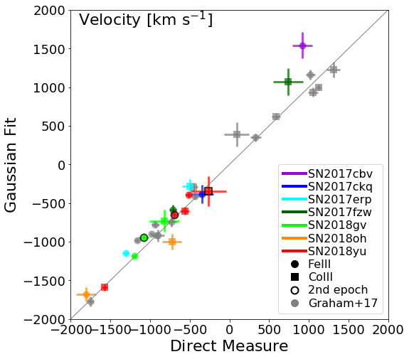
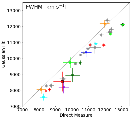
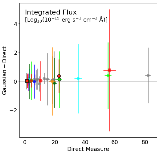
Figure 3: Comparisons of the directly measured and Gaussian fit parameters for the [Fe iii] and [Co iii] lines in the nebular spectra of our seven SNe Ia.

4 Sample Analysis

We present the derived properties of our sample of nebular-phase SNe Ia in context with other analyses in order to address some of the fundamental open questions about SNe Ia explosions. In the following sections we discuss how the nebular spectra can reveal the evolving physical state of the nebular material (§ 4.1); asymmetries in the explosion (§ 4.2); a WD-WD collision model (§ 4.3); the nature of the explosion mechanism (§ 4.4). Additionally, for our sample of SNe Ia nebular spectra, Sand et al. (in prep.) shows that the upper limits on narrow H$\alpha$ emission are up to three orders of magnitude lower than what is expected from non-degenerate companion progenitor systems (Mattila et al., 2005; Botyánszki et al., 2018; Dessart et al., 2020), which is consistent with other statistical analyses of nebular-phase SN Ia spectra that are revealing how rare a phenomenon this may be (e.g. Maguire et al., 2016; Graham et al., 2017; Sand et al., 2019; Tucker et al., 2020).

4.1 Evolution of the Nebula

The complex of iron features from $\sim$4400 to $\sim$5500 Å can be used to explore the time-changing physical state of the nebular material. For example, Black et al. (2016) focused on this iron complex in late-time spectra for over two dozen SNe Ia (although not all with spectra $>$200 days, the phases explored in this work). They used their extensive data set and synthetic model spectra to study the red-ward evolution of the $\lambda$4700Å emission line (primarily [Fe iii]), which had been noted by many past works but was not well understood. Black et al. (2016) found that in addition to changing contributions from forbidden lines (e.g., decaying ⁵⁶Co, evolving contributions of [Fe ii] and [Fe iii]), the opacity from permitted iron absorption lines played a role in this evolution. Here we add our spectra to the ongoing study of this complex of iron features.

In the top two panels of Figure 4 we compare two dozen spectra of SNe Ia at a variety of nebular phases in order to demonstrate the time evolution of the $\lambda$4700Å emission line. These spectra have been smoothed with a Savitsky-Golay filter of 100 Å, have had a pseudo-continuum at $\lambda\approx 5600$ Å subtracted, and have been flux scaled such that the $\lambda$4700Å line peak flux is $10^{-16}$ $\rm erg\ s^{-1}\ cm^{-2}\ \AA$. The spectra are colored by the phase of their observation (as in the panels’ legends), so that the red-ward evolution of the $\lambda$4700Å line stands out clearly. Vertical dashed, dotted, and solid lines in Figure 4 show the locations of [Fe iii], [Fe ii], and [Co ii], respectively.

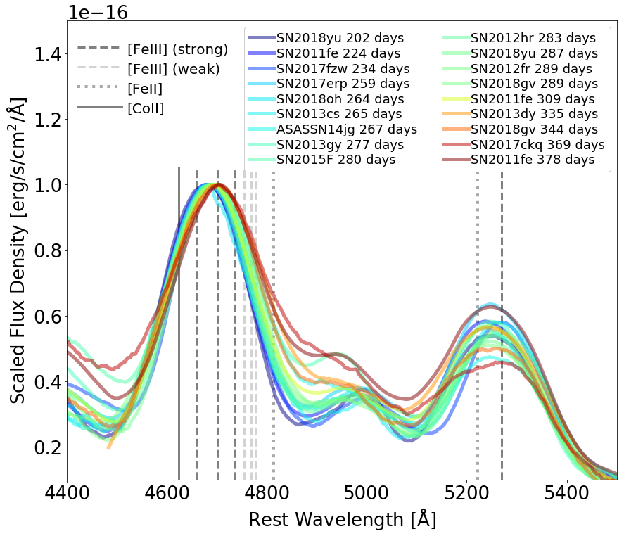
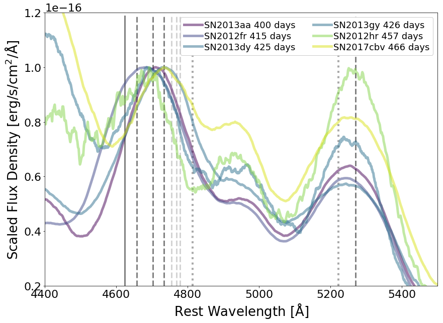
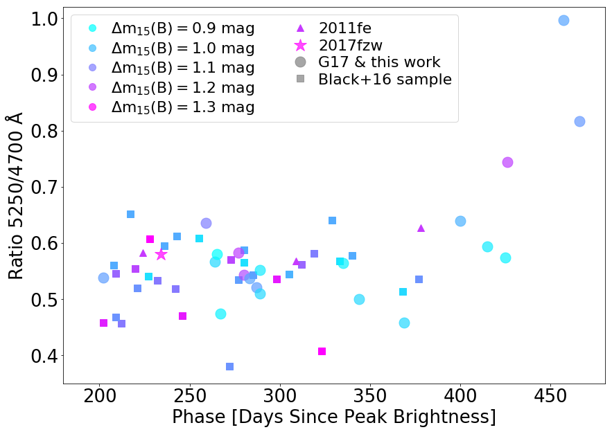
Figure 4: Top: Scaled nebular spectra from Graham et al. (2017) and this work (with spectra of SN 2011fe for comparison), shown in a color-map based on the phase as described in the lenged, in the region of the strongest [Fe iii] and [Fe ii] lines (dashed and dotted vertical lines). Middle: Similar to the top panel, but for spectra at phases $>$400 days past peak. Bottom: The ratio of the peak flux of the 5250 to the 4700 Å feature as a function of phase, with points colored by the SNe Ia light-curve decline rate, $\rm\Delta m_{15}(B)$, as described in the legend.

In the top panel of Figure 5 we show the evolution of the nebular-phase $\lambda$4700Å line velocity as a function of phase for the same spectra in Figure 4, with the sample of Black et al. (2016) also plotted for comparison. Thanks to the sensitivity of the 8m Gemini telescopes, this work is stretching the sample of nebular spectra with measurable $\lambda$4700 Å lines past $450$ days. Despite adding seven new SNe Ia to this plot, SN 2012fr remains an unique outlier in this trend, as presented in Graham et al. (2017).

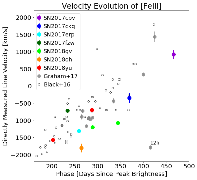
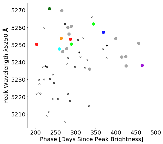
Figure 5: Top: The directly measured velocity of the [Fe iii] $\lambda$4700Å emission line as a function of phase in days since peak brightness for our Gemini nebular-phase spectra (colored symbols). Grey filled symbols represent data from Graham et al. (2017) and small open circles data from Black et al. (2016), for comparison. Bottom: The directly measured peak wavelength of the $\lambda$5250 Å iron feature as a function of phase in days since peak brightness for the same data set as above.

For the $\lambda$4700Å complex, the decline of emission from the radioactive decay of [Co ii] and, potentially, an increasing amount of [Fe ii] in the cooling nebula might at first be suspected as the culprit for the red-ward evolution of the peak (i.e., because they contribute to the blue and red sides of the feature, respectively). While they both likely do contribute, an increasing dominance of [Fe ii] would also be expected to cause a blue-ward shift in the peak of the $\lambda$5250Å line (i.e., towards the dotted line of [Fe ii] at $\lambda$5200 Å). In fact, a tentative trend in the opposite direction is seen in our plot of the $\lambda$5250Å line’s peak wavelength as a function of phase in the bottom panel of Figure 5. This red-ward shift was also shown for the nebular iron features at $\lambda{\sim}$5000 Å by Black et al. (2016). The fact that we also see it for the $\lambda$5250 feature is consistent with the measurements of Black et al. (2016), and with their conclusions that other factors, primarily opacity from the absorption by permitted lines, are the cause of the red-ward evolution exhibited by the nebular-phase iron emission features.

Aside from red-ward shifts in these iron lines’ velocities (and broadening of the FWHM, as noted in Black et al. 2016), we were curious as to whether there was a link between the relative fluxes of the $\lambda$4700 and $\lambda$5250 Å lines, and the properties of SN Ia early-time light curves. For example, if the $\lambda$5250 Å line was increasingly dominated by [Fe ii] as the ionization state of the nebula evolved, perhaps the flux ratio of the $\lambda$5250 to the $\lambda$4700 Å line would be larger at a given phase for SNe Ia that synthesized less ⁵⁶Ni. In other words, perhaps the the transition to [Fe ii] occurs earlier for less energetic, faster-cooling SN Ia nebulae.

To investigate this, in the bottom panel of Figure 4 we plot the flux ratio of the $\lambda$5250 to $\lambda$4700 Å lines as a function of phase, and color the symbols by the decline-rate parameter $\rm\Delta m_{15}(B)$, which is correlated with the peak $B$-band magnitude which is known to be a proxy for ⁵⁶Ni mass (e.g., Arnett, 1982; Phillips, 1993). In this color scheme, SNe Ia that decline slowly are cyan (i.e., synthesized more ⁵⁶Ni), and SNe Ia that decline more rapidly are magenta (i.e., synthesized less ⁵⁶Ni). In addition to the nebular-phase spectra presented in this work and in Graham et al. (2017), this plot includes the spectra analyzed by Black et al. (2016) as smaller square points.

The most obvious trend in the bottom panel of Figure 4 is the increasing $\lambda$5250/$\lambda$4700 flux ratio at phases later than 350 days. This could be due to the transition from the emission being dominated by [Fe iii] to [Fe ii] as the ionization state of the nebula evolves and the evolving temperature of the nebula (the [Fe iii] line strengths are temperature dependent). For example, the modeling work of Fransson & Jerkstrand (2015) shows that the nebula’s temperature starts a dramatic drop at about $\sim$350 days (their Figure 1) as the dominant cooling mechanism switches from optical to NIR emission lines, known as the SN Ia Infrared Catastrophe (IRC). The models of Fransson & Jerkstrand (2015) predict a plateau in the NIR light curves of SNe Ia, which was recently confirmed by observations presented by Graur et al. (2020); see also the evidence presented for the IRC based on psuedo-bolometric light-curve modeling for SN Ia 2011fe by Dimitriadis et al. (2017). Additionally, we note that this increase in the $\lambda$5250/$\lambda$4700 flux ratio at $\sim$350 days is similar in its timing to the increase in NIR to optical flux ratio shown in Maguire et al. (2018, their Figure 9). With NIR spectra for SN 2013aa at 360 and 425 days, Maguire et al. (2018, their Figure 12) also show that this increase in the NIR/optical flux ratio is due to the [Fe ii] emission lines at $\lambda$12000 and 16000 Å remaining constant while the optical emission declines. As also suggested by Maguire et al. (2018), these NIR observations support the hypothesis that the increasing $\lambda$5250/$\lambda$4700 flux ratio is due to the cooling nebula’s evolution from doubly- to singly-ionized iron.

In making the bottom panel of Figure 4 we were looking for a correlation wherein faster-declining SNe Ia (magenta points) have a higher $\lambda$5250/$\lambda$4700 flux ratio at earlier phases compared to slower-declining SNe Ia (cyan points). This trend would manifest in this plot as a magenta-to-cyan gradient from high-to-low flux ratio, and the gradient might not be strictly horizontal but might appear on an angle from upper-left to lower-right, due to a correlation between $\lambda$5250/$\lambda$4700 flux ratio and phase. Such a gradient is only very tentatively seen, and perhaps only emerges at $>$350 days, but there is also a bias here in that faster-declining (magenta) SNe Ia are not as frequently observable so late into the nebular phase. Thus we conclude that the data at hand cannot confirm or reject our hypothesis of a correlation between ⁵⁶Ni mass and the $\lambda$5250/$\lambda$4700 flux ratio as an indicator of the ionization state or temperature of the nebula. A larger number of $>$350 day spectra in future samples might help to clarify this.

4.2 Explosion Asymmetry

Maeda et al. (2010b) was the first to interpret the correlation between the photospheric velocity gradient and the velocity of the nebular-phase [Fe ii]+[Ni ii] $\lambda$7200 Å feature as a signature of explosion asymmetry. Their proposed physical model is an off-center explosion which, when aligned away the observer along their line-of-sight, results in red-shifted [Fe ii] and [Ni ii] emission lines because the bulk of the nucleosynthetic material is on the far side of the nebula. This scenario causes the SN Ia ejecta’s outer layers of the near side to be of lower density compared to the far side, and since the photosphere can recede more rapidly into this lower density material, a larger photospheric velocity gradient is observed at early times.

In the top panel of Figure 6 we plot the photospheric velocity gradient vs. the nebular velocity from the original data of Maeda et al. (2010b) as small symbols; from similar measurements presented in Silverman et al. (2013) and Graham et al. (2017) as larger symbols; and from our sample of SNe Ia as colored symbols. It is only possible to measure the velocity gradient for SNe Ia with multiple photospheric-phase spectra, but it has been shown that the velocity gradient is correlated with the photospheric velocity (as measured from the Si ii $\lambda$6355 Å absorption feature in a single spectroscopic observation near peak brightness; Benetti et al. 2005; Wang et al. 2009b; Wang et al. 2013; Silverman et al. 2013). In the bottom panel we plot the photospheric velocity versus the nebular velocity, including SNe Ia for which only a single spectrum was obtained. Measurements from Maguire et al. (2018) are shown as small symbols for comparison. We note that Maguire et al. (2018) measures the nebular velocity from the [Fe ii] $\lambda$7155 Å feature only, whereas we (and others) use an average of the [Fe ii] and [Ni ii] line velocities, and that the difference is typically only a few hundred $\rm km\ s^{-1}$.

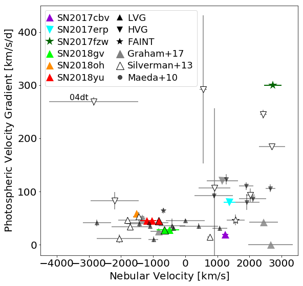
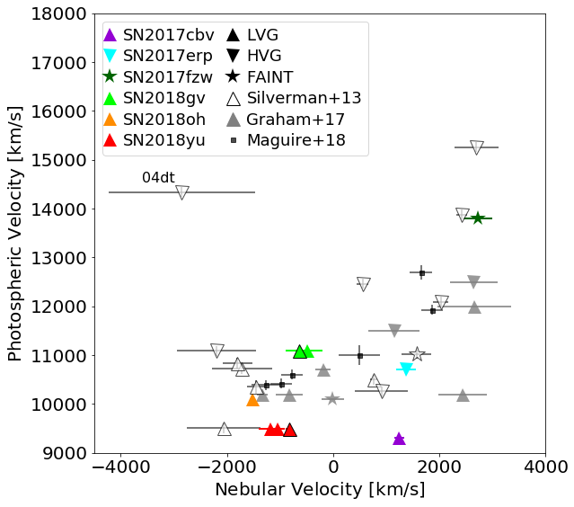
Figure 6: The photospheric velocity gradient of Si ii $\lambda$6355Å during the two weeks after peak brightness (top), and the photospheric velocity of Si ii $\lambda$6355Å near light-curve peak brightness (bottom), versus the nebular line velocity as measured using Gaussian fits to the [Fe ii] and [Ni ii] blended feature in our nebular-phase spectra from Gemini Observatory (colored symbols; a black outline indicates data from a second epoch).

It is clear from both panels of Figure 6 that SNe Ia with large photospheric velocity gradients are almost exclusively associated with red-shifted nebular-phase emission lines. These plots reinforce the previously observed correlation, and agree with the asymmetry models of Maeda et al. (2010b).

4.3 The WD-WD Collision Scenario

The head-on collision of two white dwarf stars, potentially as a result of orbital evolution driven by a distant tertiary in the system, has been proposed as a potential progenitor scenario for SNe Ia (e.g., Thompson, 2011; Katz & Dong, 2012). One predicted observable signature of a WD-WD collision scenario is bimodal emission lines in nebular phase spectra due to the ejecta from the two progenitors moving at high speeds in different directions (Kushnir et al., 2013). Dong et al. (2015) identify the [Co iii] $\lambda$5900 Å nebular feature as the best indicator of this phenomenon, because it is both a decay product of ⁵⁶Ni and does not suffer from significant contamination from other species. Depending on the viewing angle, a WD-WD collision could cause this emission line profile to appear clearly double-peaked, broadened, or single-peaked. Although none of the [Co iii] $\lambda$5900 Å emission features in our sample exhibited clear double peaks upon visual inspection (Figure 7), since the bimodality might not be obvious to the eye we apply a more stringent statistical analysis to evaluate the likelihood of double-peaked [Co iii] emission features in our spectra.

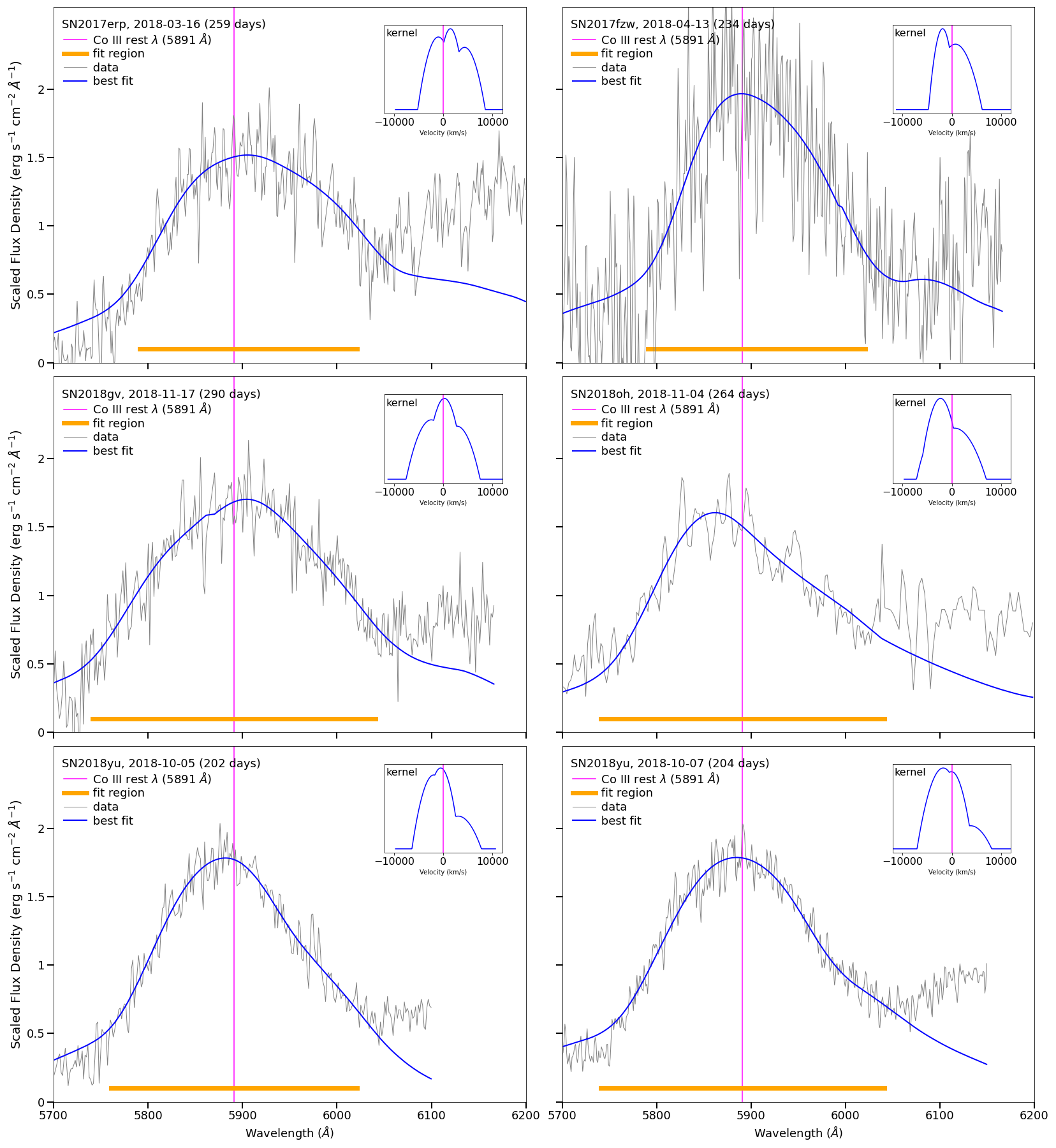
Figure 7: The convolution fits and velocity kernels (inset) for the [Co iii] lines of each of our spectra with a discernable cobalt feature (i.e., that all the cobalt had not yet decayed). To identify a SN as a bimodal candidate, the two quadratics in the kernel must be separated by more than the sum of their standard devations. All of the kernels shown above are too blended to meet that criteria.

To test our sample for [Co iii] $\lambda$5900 Å lines with two components we use a convolution fitting method similar to those used by Dong et al. (2015) and Vallely et al. (2020). We use the emcee sampler (Foreman-Mackey et al., 2013) to find the two-component kernel which, when convolved with the nebular spectrum of SN 1999by, provides a best-fit (minimum log likelihood) to the [Co iii] $\lambda$5900 Å feature in each of our spectra. The best fit results (blue lines) are shown for six spectra (grey lines) for five of our SNe Ia in the panels of Figure 7, where the orange bar denotes the fit region which begins and ends at the ‘edges’ of the [Co iii] features, and the inset panels to show the best fit bimodal kernels.

Although we find that all features can be fit with a bimodal kernel, this does not mean that they are likely to physically be bimodal. We apply the separation criteria described by Vallely et al. (2020, their Section 3): that the separation of the two components must be greater than the sum of their standard deviations. Ultimately we find that none of the best-fit kernels meet the criteria to be declared a likely indication of bimodal emission, and we are therefore unable to identify any of our objects as WD-WD collisional candidates by this metric. Our null result is consistent with the theoretical triple-system population synthesis models and evolution simulations of Toonen et al. (2018), who report that the rate of SNe Ia in triple systems is only $\sim$0.1% the total rate of SNe Ia from binary systems. However, as Vallely et al. (2020) points out, bimodal nebular-phase emission lines can be the result of asymmetric detonation, which could be much more common (e.g., Gerardy et al., 2007).

4.4 The Ni/Fe Ratio

Different explosion models for SNe Ia, such as the double-detonation (DDT) model (e.g., Seitenzahl et al., 2013) or the sub-Chandrasekhar mass (sub-$\rm M_{Ch}$) models (Sim et al., 2010; Shen et al., 2018), predict different nebular-phase Ni/Fe ratios with only a small dependence on phase, as ⁵⁶Co continues to decay and add to the amount of ⁵⁶Fe (e.g. Maguire et al., 2018, their Figure 10). The metallicity of the white dwarf progenitor star also has an impact on the nebular-phase Ni/Fe ratio: higher metallicity progenitors have more neutrons available to synthesize stable products (e.g. Timmes et al., 2003). Practically all of the nickel remaining in the nebular phase was formed stably, as ⁵⁶Ni has a half-life of 6 days and the relatively smaller amount of ⁵⁷Ni a half-life of just 35.6 hours (observations have shown that the mass ratio of ⁵⁷Ni to ⁵⁶Ni is $<$5%; Graur et al. 2016; Flörs et al. 2018).

In order to estimate the Ni/Fe ratio from our sample of nebular-phase SNe Ia spectra, we follow the example of Maguire et al. (2018) and fit the four [Fe ii] and two [Ni ii] emission features in this region: [Fe ii]$\lambda$ 7155, 7172, 7388, and 7453 Å, and [Ni ii]$\lambda$ 7378 and 7412 Å. The [Fe ii]$\lambda$ 7172, 7388, and 7453 Å features have relative intensities of 0.24, 0.19, and 0.31 compared to the 7155 Å feature, and the [Ni ii]$\lambda$ 7453 Å feature has a relative intensity of 0.31 compared to the 7378 Å feature (Jerkstrand et al., 2015). As in Section 3.4 we first fit and subtract a linear pseudo-continuum and then use the scipy.optimize.curve_fit function with six Gaussian parameters: the width, velocity, and peak of the [Ni ii] and [Fe ii] lines. The only boundary we place is on the width of the nickel lines, which is limited to $\lesssim 13000$ $\rm km\ s^{-1}$ to avoid extremely broad and shallow Gaussian features being fit (especially for the older or lower-resolution spectra). In Figure 8 we show the results of these multi-component Gaussian fits for all the spectra presented in this work. We also perform these fits for the spectra from Graham et al. (2017), but do not include them in Figure 8.

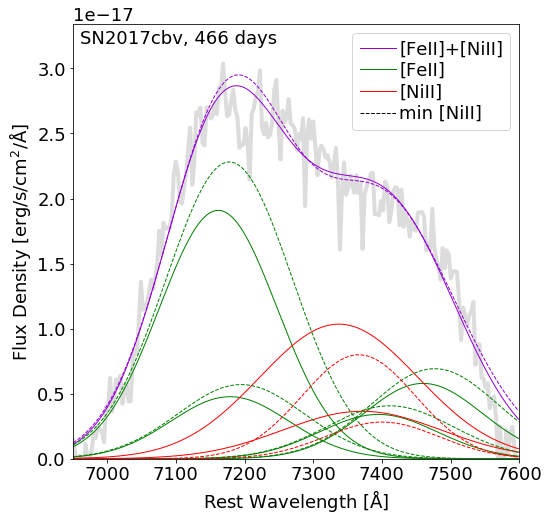
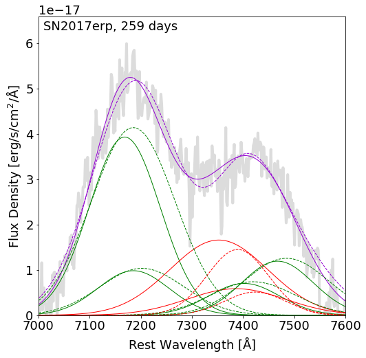
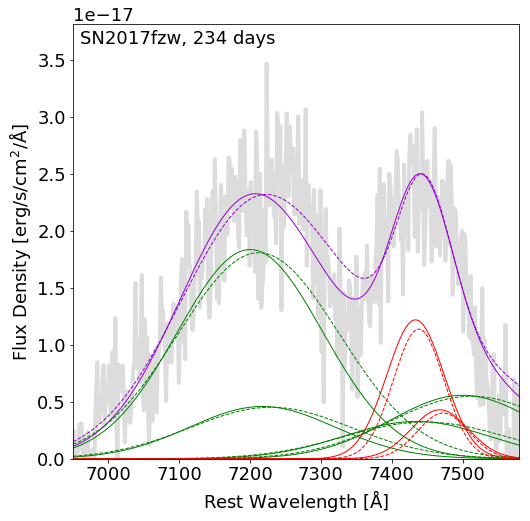
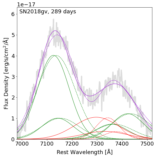
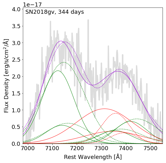
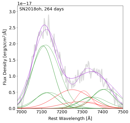
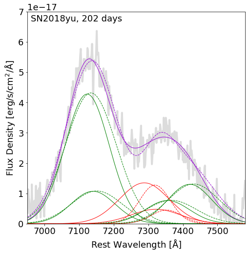
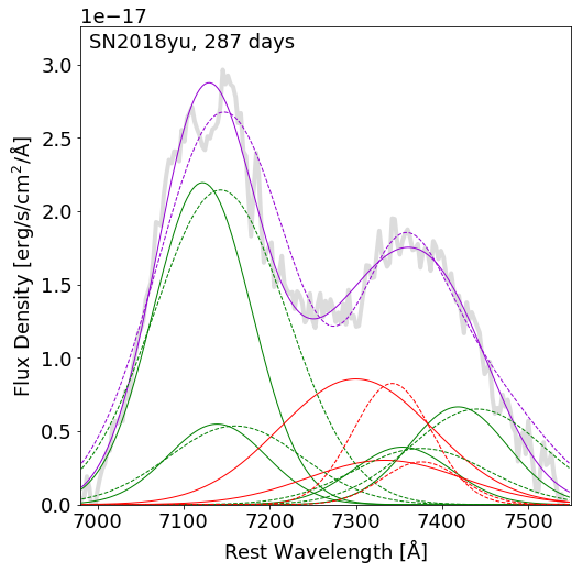
Figure 8: Multi-component Gaussian fits to the blended [Fe ii]+[Ni ii] emission feature in our nebular-phase spectra. The thick grey line is the pseudo-continuum subtracted flux density at rest wavelengths; the thick green and thin red lines show the best-fit iron and nickel features, respectively; and the purple lines show the combined best fit. The results from a simultaneous fit of iron and nickel are shown with solid lines, and the results from a two-stage fit of first iron, and then a minimum amount of nickel to the remaining flux, are shown with dashed lines.

As mentioned above, in some cases the best fits are for extremely broad nickel lines, especially for the older and lower-resolution spectra. Thus we adopt a two-stage fit method to estimate the minimum amount of nickel, and obtain a lower limit on the Ni/Fe ratio. First, we fit iron to the blue half of the feature, and then allow nickel to make up the rest of the flux in the blended feature. The results of these two-stage minimum-Ni fits are shown as dashed lines in Figure 8. It is immediately clear to the eye that in many cases fits from these two methods are generally similar (purple lines), yet can have quite different relative contributions from iron and nickel (green and red lines).

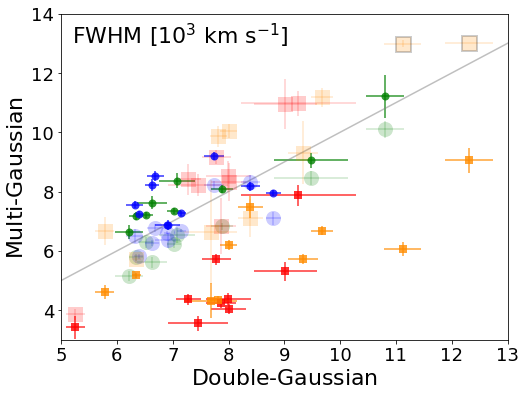
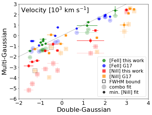
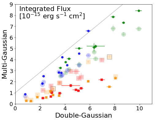
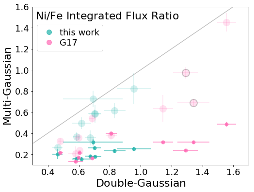
Figure 9: Panels show comparisons of the emission line parameters FWHM (top left), velocity (top right), and integrated flux (bottom left) measured from multi- and double-Gaussian fits to the [Fe ii] $\lambda$ 7155 Å and [Ni ii] $\lambda$ 7378 Å features for spectra presented in this work (green/red points) and spectra from Graham et al. (2017, G17, blue/orange points). Large transparent points represent the results of fitting iron and nickel simultaneously, whereas small opaque points represent the two-stage minimum-Ni fit method. Points with black boundaries indicate cases where the FWHM of the nickel feature reached the fit boundary of $13000$ $\rm km\ s^{-2}$. The bottom right panel compares the ratio of the integrated fluxes of the nickel and iron lines with the same stylistic conventions as the other panels.

In Figure 9 we present a four-panel comparison of the results of these multiple-component Gaussian fits to the results of our double-component Gaussian fit parameters from Section 3.4. The large transparent symbols show the results of the combined fit, whereas the smaller opaque symbols show the results of the minimum-Ni fit. The panels in Figure 9 compare the FWHM, velocity, integrated flux, and the ratio of the Ni/Fe integrated fluxes. The top two panels demonstrate how the FWHM of nickel is broader, and the velocity of nickel is bluer, when the nickel and iron are fit simultaneously; i.e., when nickel is allowed to contribute to the blue-half of the feature (large transparent points). The top left panel also shows that the nickel and iron have more similar velocities from the two-stage fit method (small opaque points). This suggests the minimum-Ni method might be more accurate in some cases, because a significantly broader/bluer velocity for nickel compared to iron is not expected (e.g., as shown in Figure 4 of Mazzali et al. 2015). We emphasize that the incorporation of the minimum-Ni line-fitting method is not motivated by a desire to challenge the existence of stable Ni in the nebular SN Ia material, the presence of which is well-established (e.g., Blondin et al., 2021), but by our need to obtain a lower limit on the Ni/Fe ratio (Figure 10) to inform our discussion of SN Ia explosion models, below.

The bottom-left panel of Figure 9 demonstrates how the minimum-Ni fitting method (small opaque points) does in fact lead to minimal flux in the nickel component, by design. Note that because the multi-Gaussian fit measures of integrated flux only include the primary lines, [Fe ii] $\lambda$ 7155 Å and [Ni ii] $\lambda$ 7378 Å, their fluxes are systematically lower than those from the double-Gaussian fit, which includes all lines. The bottom-right panel shows that the Ni/Fe ratio is systematically lower for a multi-Gaussian fit compared to the double-Gaussian fit. This is primarily due to proper accounting for iron contributions in the red-half of the feature, which are attributed to nickel in the double-Gaussian fit. We can also see that the minimum-Ni fitting method (small opaque points) leads to significantly lower Ni/Fe ratios, also by design.

Instead of integrated flux, Maguire et al. (2018) use the ratio of the pseudo-equivalent width (pEW) of the [Fe ii] $\lambda$ 7155 Å and [Ni ii] $\lambda$ 7378 Å features to estimate the Ni/Fe abundance ratio. We measure the pEW for the 7378 Å and 7155 Å features in the SN Ia spectra presented in this work, and from Graham et al. (2017). In Figure 10 we show the Ni/Fe pEW ratio as a function of phase, and compare with those from Maguire et al. (2018, their Table 3). As in Figure 8, we use larger transparent symbols to represent the simultaneous fit of iron and nickel, and smaller opaque symbols to represent the two-stage minimum-Ni fit. It is clear that the errors on the Ni/Fe pEW ratio are underestimated: there are a few cases of measurements from different spectra of the same object (e.g., SNe Ia 2013aa, 2013cs, 2018gv, and 2018yu) which differ by more than the error. However, the greater problem is that the minimum amount of nickel required to fit the blended [Fe ii]+[Ni ii] feature is significantly lower than the amount of nickel that can be fit, leading to a lot of scatter in the $y$-axis of Figure 10.

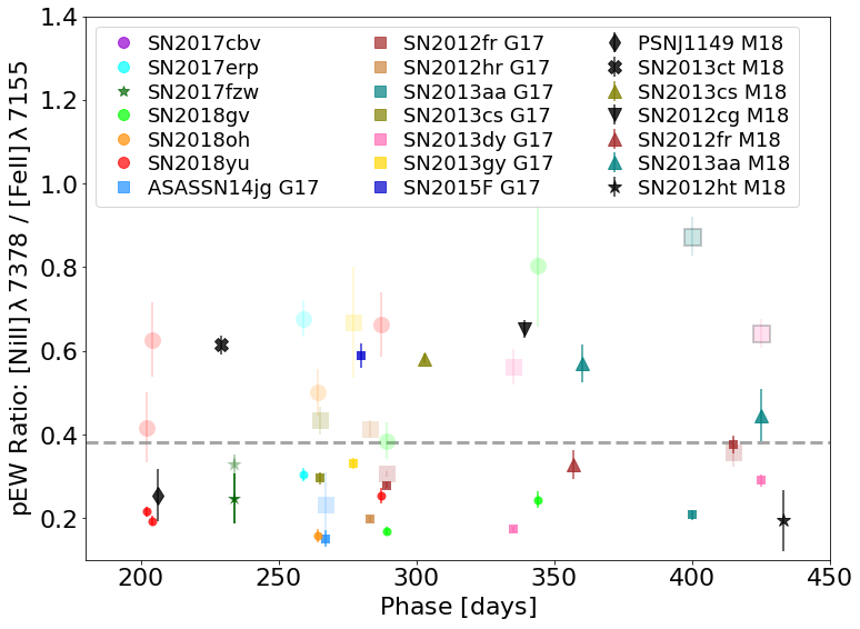
Figure 10: The ratio of the pseudo-equivalent widths (pEW) of iron and nickel as a function of phase for SN Ia. Data come from the current work, as well as Graham et al. (2017, G17), and Maguire et al. (2018, M18, their Table 3). Large transparent points represent the simultaneous fit results, and small opaque points the minimum-Ni fit results. Note that the Ni/Fe pEW ratio of SN 2015F from the simultaneous fit method lies off the plot ($\sim 1.75$ at 280 days). The dashed horizontal line, as in Maguire et al. (2018, their Figure 10), is at the solar Ni/Fe ratio and also marks the approximate division between predictions for the Ni/Fe ratio from delayed detonation (DDT) models and high-metallicity sub-$\rm M_{Ch}$ models (above the line) and lower-metallicity sub-$\rm M_{Ch}$ models (below the line).

Specifically, the problem is that for most of the SNe Ia in our sample (but not all – see Section 4.4.1), the results of the simultaneous fit and the minimum-Ni fit methods lie above and below the dashed line in Figure 10, respectively. This dashed line is the same as that shown in Maguire et al. (2018, their Figure 10). This line represents the solar Ni/Fe ratio, and also coincides with the approximate division between model predictions: above the line are Ni/Fe ratios from delayed detonation (DDT) models (Seitenzahl et al., 2013) and super-solar metallicity ($\gtrsim$3–6$\times$) sub-$\rm M_{Ch}$ models (Sim et al., 2010; Ruiter et al., 2013); below the line are Ni/Fe ratios from lower-metallicity ($\lesssim 2$ $\rm M_{\odot}$) sub-$\rm M_{Ch}$ models (Shen et al., 2018).

Thus, the degeneracy between iron and nickel contributions to the blended feature precludes us from drawing any general conclusions about the physical nature of the explosion mechanism based on our optical nebular phase spectra alone. Future data sets which have higher resolution, better SNR, and/or nebular-phase NIR spectra – in which relatively isolated [Fe ii] features could be used to better constrain the iron line parameters – might offer improvements in the effort to physically constrain SNe Ia models. We furthermore direct the reader to the work of Flörs et al. (2020), who apply full spectral synthesis models to optical-NIR nebular-phase spectroscopy. They are able to draw much more robust conclusions for their entire sample, finding that the majority of Ni/Fe ratios for SNe Ia align with predictions of the sub-Chandrasekhar mass models (i.e., fall below the dashed line in our Figure 10). That type of analysis is beyond the scope of this work.

4.4.1 Five SNe Ia with truly low Ni/Fe ratios

In our sample of SNe Ia there are three with Ni/Fe ratios that are consistently below the dashed line in Figure 10: SN 2017fzw, ASASSN-14jg, and SN 2012fr. In addition, Maguire et al. (2018) find that PSNJ1149 and SN 2012ht have low Ni/Fe ratios. Thus it likely that these five SNe Ia have truly low Ni/Fe ratios, and consider them as candidates for sub-$\rm M_{Ch}$ mass and/or lower-metallicity progenitors. Two of these events, 2012ht and 2017fzw (both represented with 5-point star symbols in Figure 10), are transitional SNe Ia which exhibit some signatures of 91bg-likes, such as faint peak magnitudes and quicker decline rates (larger $\Delta m_{15}(B)$ values). Transitional SNe Ia may experience a different explosion mechanism and are discussed further in Section 5.4. No published or publicly available photometric data can be found for PSNJ1149, which was spectroscopically classified as a normal SN Ia by Rudy et al. (2015).

The other two of these events, SN 2012fr and ASASSN-14jg, have similar $\Delta m_{15}(B)$ parameters of $0.93$ and $0.92$ mag, and similar peak $B$-band brightnesses of $-19.4$ and $-19.3$ mag, respectively (Graham et al., 2017). SN 2012fr exhibited a low velocity gradient (LVG; but did have a high Si ii velocity at peak, $12000$ $\rm km\ s^{-1}$, Graham et al. 2017), and ASASSN-14jg a low velocity, in their photospheric Si ii absorption feature from spectra obtained near and shortly after peak brightness. They also both exhibit red-shifted velocities for the [Fe ii]+[Ni ii] nebular emission feature. Perhaps the detonation of a lower-density, sub-$\rm M_{Ch}$ progenitor which spread through a greater volume of the white dwarf – compacting the outer layers all around to exhibit an LVG for its Si ii – but that was still offset ‘away’ from the observer to exhibit red-shifted nebular lines could explain these observations. A detonation in a larger volume of the white dwarf could also generate more ⁵⁶Ni, which could cause the slightly over-luminous light curves (and lower decline rates) for 2012fr and ASASSN-14jg, and potentially also the lower Ni/Fe ratio at late times. As previously mentioned, metallicity could also play a role here: lower (higher) metallicity white dwarfs could produce relatively less (more) stable nucleosynthetic products due to the under (over) abundance of neutrons (Timmes et al., 2003). Although both SN 2012fr and ASASSN-14jg have spiral host galaxies and are thus candidates for having higher-metallicity progenitors, they could have originated from the spirals’ metal-poor stellar populations. Ultimately, with the data at hand it is not possible to separate the various potential factors involved, or to definitively pin the low Ni/Fe ratio on a single underlying cause.

5 Discussion of Individual Objects

In Sections 5.1 to 5.7 we explore the physical implications of the early-time data and nebular-phase spectra for each of our individual objects.

5.1 SN 2017cbv, a “Blue Bump" SN Ia

5.1.1 Early-time SN 2017cbv

Hosseinzadeh et al. (2017a) discovered SN 2017cbv in the outskirts of spiral galaxy NGC 5643 at $z=0.00399$ (Koribalski et al., 2004) by the Distance Less Than 40 Mpc (DLT40; Tartaglia et al. 2018) survey on Mar 10.14 2017 UT with an apparent magnitude of $R=15.6$ (Tartaglia et al., 2017). SN 2017cbv was spectroscopically classified as a young Type Ia SN based on an optical spectrum from the Las Cumbres Observatory FLOYDS-S spectrograph on Mar 10.7 2017 UT (Hosseinzadeh et al., 2017b), with a good fit to the peculiar SN 1999aa, Garavini et al. 2004. Light curve fitting by Hosseinzadeh et al. (2017a), who assume that SN 2017cbv experienced a host galaxy extinction of $E(B-V)_{\rm host}\approx 0$ based on its remote location and lack of Na i D absorption in higher resolution spectra (Ferretti et al., 2017), finds that SN 2017cbv reached a peak magnitude of $B=11.72$ mag on Mar 29.1 2017 UT, and exhibited a decline rate of $\Delta m_{\rm 15,B}=1.06$ mag. A re-analysis of the light curve by Sand et al. (2018a) shows that the peak intrinsic magnitude was $M_{B}\approx-19.25$ mag, somewhat fainter than its spectral match, the peculiar SN 1999aa (which exhibited $M_{B}\approx M_{V}\approx-19.8\pm 0.2$ mag and $\Delta m_{15}(B)\approx 0.746\pm 0.02$ Krisciunas et al. 2000). Wee et al. (2018) also show that the width and luminosity of 2017cbv’s light curve is consistent with the Phillips relation (Phillips, 1993; Hicken et al., 2009). A further analysis of SN 2017cbv’s light curve by Burns et al. (2020) also matches with the re-analysis of Wee et al. (2018), indicating that SN 2017cbv was a normal SN Ia.

However, SN 2017cbv was special in one respect: Hosseinzadeh et al. (2017a) show that the early-time light curve of SN 2017cbv exhibited a “blue bump" during the first five days. “Blue bumps" at early times could be due to the ejecta interacting with a non-degenerate binary companion star or its CSM (Kasen, 2010), or due to the mixing of ⁵⁶Ni to the outer layers of the ejecta (Piro, 2012). Hosseinzadeh et al. (2017a) find that the “blue bump" of SN 2017cbv is consistent with the predicted signature of the SN’s ejecta impacting a non-degenerate companion star along the line-of-sight, but alternate explanations such as interaction with nearby circumstellar material (CSM) or the mixing of ⁵⁶Ni to the outer layers of the ejecta could not be ruled out. They also show that the very early optical spectra of 2017cbv exhibited strong C ii absorption and appeared more similar to the normal SN 2013dy than SN 1999aa.

5.1.2 Late-time SN 2017cbv

The nebular-phase spectrum for SN 2017cbv at $466$ days after peak brightness is shown in the top-left panel of Figure 2. For comparison, two late-time spectra of the normal SN 2011fe at phases $378$ and $574$ days past peak are also shown (these are $-88$ and $+108$ days relative to the SN 2017cbv spectrum). As expected, the peak flux of SN 2017cbv’s [Fe iii] $\lambda\sim 4700$ Å line appears to be intermediate between those of the two SN 2011fe spectra, and SN 2017cbv’s [Co iii] line has declined beyond visibility, similar to SN 2011fe’s $574$-day spectrum.

SN 2017cbv’s early-time “blue bump" suggests that we might see late-time H$\alpha$ emission if this feature is due to a non-degenerate binary companion. Sand et al. (2018a) present nebular spectroscopy at $\sim$300 days after peak brightness of SN 2017cbv and constrain the mass of hydrogen in the system to $\leq 10^{-4}$ $\rm M_{\odot}$. This limit is about three orders of magnitude lower than predicted by models in which a non-degenerate companion star’s hydrogen is swept up in the SN Ia ejecta (e.g. Botyánszki et al., 2018). Additionally, Tucker et al. (2020) find no evidence of stripped companion emission for SN 2017cbv.

The lack of H$\alpha$ in the nebular-phase spectrum of SN 2017cbv might suggest that mixing of ⁵⁶Ni into the outer layers of the ejecta is more likely as the root cause of the “blue bump". The presence of ⁵⁶Ni at higher velocities could lead to broader nebular-phase lines for the nucleosynthetic decay products, which we can check with our nebular-phase spectrum. In Tables 7 and 8 (in Appendix A) we report that the iron and nickel lines exhibit a FWHM of $8100$ to $9500$ $\rm km\ s^{-1}$, which are average values and not especially broad. At 466 days the cobalt is too weak to be included in this line-width analysis, so instead we directly measure the width of the [Co iii] $\lambda$5890 Å feature in the 302 day spectrum from Sand et al. (2018a), and find a FWHM of $\sim$10400 $\rm km\ s^{-1}$, which is about a median value of FWHM for our sample (see the middle panel of Figure 3). The caveat here is that average-width nebular lines are not strong evidence against ⁵⁶Ni mixing, because observed spectral parameters are degenerate with other physical qualities, such as the density profile (Botyánszki & Kasen, 2017). Additional (and more reliable) evidence against ⁵⁶Ni mixing is that it could cause increased line blanketing in the weeks around peak brightness, depressing the luminosity especially in the bluer filters, which was not observed. In general we find no direct evidence in our nebular-phase spectrum that ⁵⁶Ni mixing was the root cause of the “blue bump".

Alternatively, early-time “blue bumps" might be a signature of the sub-$\rm M_{Ch}$ double detonation model (Noebauer et al., 2017). As discussed in Section 4.4, the Ni/Fe ratio in nebular-phase SN Ia spectra can be used to distinguish between the delayed detonation and (low-metallicity) sub-$\rm M_{Ch}$ model. As we were unable to robustly measure the Ni/Fe ratio for our 466 day spectrum of SN 2017cbv, we applied the multi-component Gaussian fits used in Section 4.4 to the 302 day spectrum of SN 2017cbv from Sand et al. (2018a). We found a Ni/Fe ratio of $\sim$0.6 from the best fit, and of $\sim$0.14 from the minimum-Ni fit method. These values lie above and below the Ni/Fe ratio of $\sim$0.4 which approximately distinguishes delayed detonation and (low-metallicity) sub-$\rm M_{ch}$ models (Figure 9). Thus, no conclusions about the potential connection between SN 2017cbv’s “blue bump" and its explosion mechanism can be drawn from the nebular-phase spectra.

5.2 SN 2017ckq, a Potential HVG SN Ia

5.2.1 Early-time SN 2017ckq

SN 2017ckq was discovered on 2017-03-27 UT at 18.11 mag (AB in the cyan-ATLAS filter; Tonry et al. 2017), and was classified as a Type Ia with an optical spectrum from the ESO New Technology Telescope (Gutierrez et al., 2017). It is located in host galaxy ESO-437-G-056 at $z=0.01\pm 0.001$ (Mould et al., 2000) with a Tully-Fisher distance modulus of $33.2\pm 0.2$ mag and a distance of $42.9$ Mpc (Tully et al., 2013). The Las Cumbres optical photometry that we obtained around the time of peak brightness indicates a $B$-band decline rate of $\Delta m_{\rm 15}(B)\approx 0.96\pm 0.2$ mag and an intrinsic peak brightness of $M_{B}\approx-18.9\pm 0.3$ mag (Section 2.1). Both the peak brightness and decline rate are on the low side, but given the uncertainties they are not inconsistent with the Phillips relation (Phillips et al., 1999), and so SN 2017ckq appears to be a normal SN Ia. We also found that SN 2017ckq exhibited a photospheric Si ii absorption feature with high velocity and a high velocity gradient (Table 2), and classified it as a potential HVG event (Table 2).

5.2.2 Late-time SN 2017ckq

As a potentially HVG event, we expect the nebular-phase spectrum of SN 2017ckq to exhibit a redshifted [Fe ii]+[Ni ii] feature in accordance with the asymmetric explosion model discussed in Section 4.2. Unfortunately, we only obtained a partial (blue-side) optical nebular spectrum of SN 2017ckq at 369 days after peak brightness (top-right panel of Figure 2), which does not include the [Fe ii]+[Ni ii] nebular feature. From Figure 2 we see that the blue-side features of SN 2017ckq resemble SN 2011fe, except for the noticeably flatter shape in the peak of the Fe $\lambda$5250 Å feature.

A unique aspect of the $\lambda$5250 Å feature for SN 2017ckq also manifests in the top panel of Figure 4, in which SN 2017ckq has the distinction of exhibiting the lowest 5250/4700 flux ratio of all the SNe Ia in that sample. The $\lambda$5250 Å feature is a blend of [Fe ii] and [Fe iii], whereas the $\lambda$4700 Å feature is primarily [Fe iii]. As described in Section 4.1, the 5250/4700 flux ratio appears to rise in spectra $>$350 days after peak brightness, which could be due to the nebula cooling and the ionization state transitioning from doubly- to singly-ionized iron. We hypothesized that SNe Ia with larger ⁵⁶Ni masses (and lower light-curve decline rates) might exhibit a lower 5250/4700 flux ratio for longer into the nebular phase due to a longer cooling timescale and/or a later transition in the ionization state. By exhibiting the lowest 5250/4700 flux ratio of all the SNe Ia in our sample, exhibiting that ratio at $>$350 days past peak brightness, and also exhibiting $\Delta m_{15}(B)\sim 0.96\pm 0.2$ mag at early times, SN 2017ckq fits the hypothesis. However, the other HVG SNe Ia considered in Figure 4 (SNe 2012hr, 2013cs, and 2017erp) do not exhibit this flattened shape for the $\lambda$5250 Å feature, and neither do any of the other spectra in this sample (nor in the sample of Graham et al. 2017). The physical origin of the flattened shape of SN 2017ckq’s $\lambda$5250 Å feature remains unclear.

5.3 SN 2017erp, an NUV-Red High-Velocity SN Ia

5.3.1 Early-time SN 2017erp

SN 2017erp was discovered on 2017-06-13 UT at 16.8 mag (Vega; clear filter) by K. Itagaki (Itagaki, 2017), and classified as a Type Ia in NGC 5861 at $z=0.006174$ (Theureau et al., 2005) with an optical spectrum from the South African Large Telescope (Jha et al., 2017). Brown et al. (2019) present an analysis of 2017erp with UV and optical photometry and spectra spanning the first $\sim 120$ days after explosion. They find that SN 2017erp exhibited a light curve apparent peak brightness of $m_{B}=13.27\pm 0.01$ mag and decline rate of $\Delta m_{\rm 15}(B)\approx 1.1$ mag. Brown et al. (2019) provide an extensive analysis of the light curve shape and color, which we summarize as indicating a host-galaxy extinction of $A_{V}\approx 0.45\pm 0.05$ mag. This, along with the host’s distance modulus $\mu=32.34\pm 0.097$ mag (Könyves-Tóth et al., 2020), suggests a peak intrinsic magnitude of $B\approx-19.5\pm 0.15$ mag. We note also that Könyves-Tóth et al. (2020) report a synthesized ⁵⁶Ni mass of $0.975\pm 0.083$ $\rm M_{\odot}$, the highest in their sample of 17 SNe Ia. Altogether, SN 2017erp was a normal, slightly overluminous Type Ia in terms of its optical light curve shape and spectra.

After their careful evaluation of the host galaxy’s contribution to the line-of-sight extinction and reddening, Brown et al. (2019) show that SN 2017erp exhibited a depressed NUV flux and an intrinsically redder NUV-optical color than other SNe Ia, such as the NUV-blue SN 2011fe. They suggest that this might indicate that the progenitor of SN 2017erp had a higher progenitor metallicity than SN 2011fe, but note that mixing of nucleosynthetic products into the outer layers cannot be ruled out. Brown et al. (2019) demonstrate how the spectra of SN 2017erp prior to peak brightness exhibit a high-velocity Si ii ${\lambda}6355$ Å feature and a C ii ${\lambda}6580$ Å feature which disappears by phase $-12$ days. They also show how the photospheric velocity is higher than 2011fe at early times, but declines to be of a similar value by peak brightness (their Fig. 9). With spectroscopy from Las Cumbres Observatory, we have classified SN 2017erp as a potential member of the HVG-class (Table 2).

5.3.2 Late-time SN 2017erp

If SN 2017erp had a higher progenitor metallicity, the additional neutrons available might lead to a higher ratio of stable-to-radioactive iron and nickel in the nucleosynthetic products (e.g., Timmes et al., 2003). During the nebular phase, all of the radioactive nickel has decayed and only stable nickel remains, and so a higher progenitor metallicity could manifest in our nebular-phase spectrum as a higher Ni/Fe ratio than in typical SNe Ia. However, in Figure 2 (second-row left panel) we can see that the Ni/Fe ratio exhibited by the nebular-phase spectrum of SN 2017erp is similar to that of the typical SN 2011fe at a similar phase. Furthermore, as described in Section 4.4 we find a significant degeneracy in the relative contributions of nickel and iron that can provide good fits to the $\lambda$7200 Å Ni+Fe blended feature (as is the case for most of the SNe Ia in our sample). Thus, the nebular-phase spectra of SN 2017erp do not help to confirm or reject the hypothesis of a higher progenitor metallicity.

If the depressed NUV flux of SN 2017erp was instead due to the mixing of nucleosynthetic products to the outer layers, where it could absorb the NUV photons, then we might expect to find particularly broad nebular-phase emission lines. As shown in Tables 7 and 8 in Appendix A, SN 2017erp’s nebular-phase emission lines of [Fe iii] and [Co iii] were of average width, but as previously mentioned (Section 5.1.2), average-width lines are not strong evidence against mixing. In general, we find that SN 2017erp exhibited a typical, SN 2011fe-like nebular-phase spectrum, and that we are unable to draw any further conclusions about the physical origin of its depressed NUV flux.

SN 2017erp is one of the few SNe Ia which exhibited a high velocity gradient for its photospheric Si ii absorption feature in the two weeks after peak brightness. The explosion asymmetry model of Maeda et al. (2010a) suggests that detonations which are offset away from the observer along the line of sight can lead to both a photospheric-phase HVG and a nebular-phase redshift in the [Fe ii]+[Ni ii] $\lambda$7200 Å blended feature (Section 4.2). The nebular-phase spectra for SN 2017erp (Figure 2, second-row left panel) shows that this Fe+Ni feature is redshifted for SN 2017erp compared to SN 2011fe. The location of SN 2017erp in the plot of photospheric velocity gradient versus nebular-phase line velocity (Figure 6) furthermore demonstrates that SN 2017erp is consistent with the trend exhibited by SNe Ia in general, and that observations of SN 2017erp support the asymmetric explosion model.

5.4 SN 2017fzw, a Subluminous Transitional SN Ia

5.4.1 Early-time SN 2017fzw

SN 2017fzw was discovered on 2017-08-09 by Valenti et al. (2017) at 17.17 mag (AB; clear filter) as part of the DLT40 survey. It was spectroscopically classified as a 91bg-like SNe Ia using the FLOYDS-S instrument of the Faulkes Telescope South (Hosseinzadeh et al., 2017c). SN 2017fzw is located in the outskirts of NGC 2217 ($\sim$100″ from the host galaxy’s center), a face-on barred spiral at $z=0.0054$ (de Vaucouleurs et al., 1991) with a Tully-Fisher distance modulus of $31.45\pm 0.4$ mag and a distance of $19.5$ Mpc (Tully, 1988).

At early times SN 2017fzw is similar to the class of SNe Ia that resemble the underluminous, spectroscopically peculiar, fast-evolving SN 1991bg (“91bg-likes"; Filippenko et al. 1992). Galbany et al. (in prep.) presents a full analysis of SN 2017fzw and shows that it peaked on 2017-08-22.9 UT with apparent magnitudes of $B\sim 13.25\pm 0.16$ and $V\sim 13.09\pm 0.02$ mag, and a peak color of $B-V=0.17\pm 0.16$ mag. Galbany et al. (in prep.) applies corrections for both MW and host galaxy extinction, the latter with $E(B-V)_{\rm host}=0.182$ and $R_{V,\rm{host}}=3.1$, which a pretty high host galaxy extinction given its location in the outskirts (Figure 1). They furthermore show that the light curve of SN 2017fzw exhibited a decline rate of $\Delta m_{15}(B)=1.60\pm 0.02$ mag, and that light-curve fits indicate a distance modulus of $\mu=32.06\pm 0.03$ mag, which implies an absolute $B$-band intrinsic magnitude of $-18.81\pm 0.18$ mag – at the luminous end of the 91bg-like class. These values from Galbany et al. (in prep.) are quoted in Table 2, and used in our analysis.

In early-time optical spectra within $\sim$10 days of peak brightness, 91bg-like SNe Ia are distinguished by deep titanium absorption features at $\lambda$4200 Å (e.g., Mazzali et al., 1997; Taubenberger, 2017). In Figure 11 we plot a time series of phase-matched spectra of normal SN 2011fe (blue; Mazzali et al. 2015, 2014; Pereira et al. 2013; Parrent et al. 2012), SN 2017fzw (green; Galbany et al. in prep.), and SN 1991bg (red; Filippenko et al. 1992; Turatto et al. 1996). The titanium feature at $\lambda$4200 Å is most clearly seen for SNe 2017fzw and 1991bg in the top set of spectra, at phases of -10 and 0 days respectively.

5.4.2 Late-time SN 2017fzw

Nebular-phase spectra of 91bg-like events are rarely obtained because they are intrinsically less luminous and their brightness declines rapidly (Taubenberger, 2017), which makes our 234-day spectrum of SN 2017fzw both unique and valuable. There are two additional things to note about our nebular spectrum of SN 2017fzw: (1) It does not exhibit a nebular-phase emission feature at $\lambda{\sim}6300$ Å like those seen for subluminous SN 2002es-like supernovae, which has been suggested to be due to [O i] and associated with the violent merger model (e.g., Taubenberger et al., 2013; Kromer et al., 2016). (2) It was also used by Sand et al. (2019) to show that SN 2017fzw did not exhibit any late-time H$\alpha$ emission which might suggest a non-degenerate companion, as found for the subluminous SN Ia ASASSN-18tb (Kollmeier et al., 2019; Vallely et al., 2019). Additionally, Tucker et al. (2020) find no evidence of stripped companion emission for SN 2017fzw.

As shown in Figure 11, at later phases SN 2017fzw evolves away from exhibiting 91bg-like features and develops characteristics similar to the normal SN 2011fe. Specifically, the nebular-phase emission lines of 91bg-like SNe Ia become narrower over time, with typical dispersion velocities around or below $2000$ $\rm km\ s^{-1}$ (Mazzali & Hachinger, 2012). This narrowing is seen in the spectra for SN Ia 1991bg at 91 and 203 days in Figure 11, but in contrast, SN 2017fzw exhibits emission lines of comparable width to SN 2011fe in its nebular phase. This similarity of SN 2017fzw to SN 2011fe at late times is also demonstrated by the middle-right panel of Figure 2.

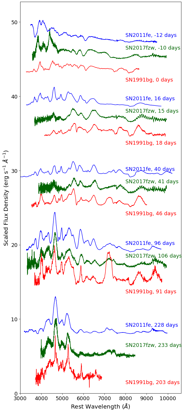
Figure 11: A time-series of phase-matched spectra for normal SN 2011fe (blue), transitional SN Ia 2017fzw (green), and the canonical sub-luminous SN 1991bg (red), from early to late times (top to bottom). Fluxes have been scaled and offset to enable the comparison. In the earliest spectra SN 2017fzw resembles SN 1991bg but by the nebular phase epoch ($\geq$200 days) it resembles SN 2011fe.

Based on the optical light curve and spectroscopic evolution of SN 2017fzw, both this work and Galbany et al. (in prep.) find that it is similar in many respects to “transitional" SNe Ia, which is the term used for SNe Ia that exhibit signatures similar to both 91bg-like and normal events, such as the transitional SN Ia 1986G (Phillips et al., 1987; Ashall et al., 2016). The term ‘transitional’ is used to refer to SNe that are in between two classes, and the SNe Ia which are ‘transitional’ between 91bg-like and normal also appear to be transitional in the sense that their spectra transition from being more 91bg-like at early times (exhibiting titanium) to more normal during the nebular phase (exhibiting broader iron features than SN 1991bg, and weaker calcium; e.g., SN 2012ht, Maguire et al. 2018; and 2015bp, Srivastav et al. 2017).

5.4.3 SN 2017fzw in Context: Normal, Transitional, and 91bg-like SNe Ia

Mazzali & Hachinger (2012) and Mazzali et al. (2011) model the nebular spectra of SN Ia 1991bg and the transitional SN Ia 2003hv, respectively, and find that a lower mass and/or density of the inner regions provides the best explanation for their late-time emission features. However, for transitional SN Ia 2003hv, their model is reproducing a large [Fe iii]:[Fe ii] flux ratio, whereas the [Fe iii]:[Fe ii] flux ratio for 2017fzw is not dissimilar to 2011fe or other normal SNe at its epoch (Figure 11, and the top panel of Figure 4). The spectral evolution for SN 2017fzw presented above leads to a hypothesis that the physical qualities that cause a transitional SN Ia to appear 91bg-like at early times might originate in the white dwarf’s outer layers, and not in its nucleosynthetic products.

To confirm or reject this hypothesis, and to explore the similarity of transitional SN Ia 2017fzw’s nucleosynthetic products with normal SNe Ia, in Figure 12 we compare the velocity dispersion of the [Co iii] $\lambda$5800 Å emission feature for a sample of normal, transitional, and 91bg-like SNe Ia. This [Co iii] feature is a good signature of the nucleosynthetic products in part because it is generally free of contamination from other species until very late phases, $>$1000 days, when sodium might contribute (Dessart et al., 2014; Graham et al., 2015b). In Figure 12 we show, from top to bottom, the [Co iii] $\lambda$5800 Å emission feature for 91bg-like, transitional, and normal SNe Ia, ordered from narrowest to broadest emission. Figure 12 shows that SN 2017fzw exhibits the broadest [Co iii] nebular emission line of all the 91bg-like and transitional SNe Ia in this sample, and that it resembles normal SN Ia 2011fe. As a side note, Vallely et al. 2020 classifies the [Co iii] feature of transitional SN 1986G as tentatively bimodal, after accounting for the Na i D absorption feature seen near ${\sim}1000$ $\rm km\ s^{-1}$. However, we find no evidence of bimodality in the [Co iii] emission of SN 2017fzw (Section 4.3).

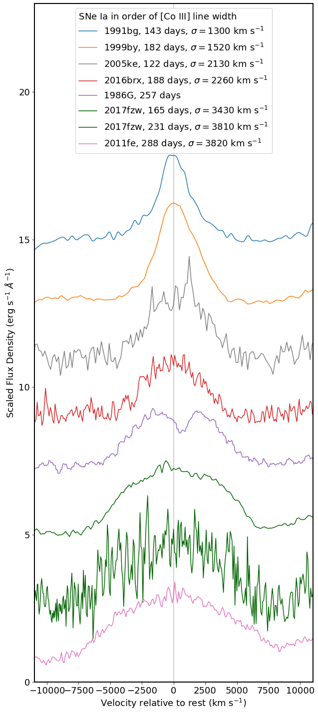
Figure 12: The nebular-phase [Co iii] $\lambda$5250 Å feature for a sample of 91bg-like (91bg, 99by, 05ke, 16brx) and transitional (86G, 17fzw) SNe Ia, and the normal SN 2011fe, ordered by increasing line width from top to bottom. Fluxes have been scaled and offset for visibility, and the line widths are provided in the legend. The transitional SN 2017fzw (green) exhibits a [Co iii] feature which is almost as broad as that of normal SN 2011fe (pink), and is dissimilar to the 91bg-like events.

To further explore SN 2017fzw in the context of 91bg-like, transitional, and normal SNe Ia, we consider its location in two phase-space diagrams which compare nebular-phase emission line widths to early-time light curve properties. In the top panel of Figure 13 we plot the light-curve decline rate parameter $\Delta m_{15}(B)$ as a function of the FWHM of the [Fe iii] $\lambda$4700 Å emission feature (as in Blondin et al., 2012, their Figure 22). This plot includes data for SNe Ia from Blondin et al. (2012), Silverman et al. (2013), Ganeshalingam et al. (2010), and Graham et al. (2017), along with the SNe Ia presented in this work. SNe Ia that are classified as 91bg-like or transitional are individually labeled, while SN 2017fzw is represented as a five-point star. Compared to the normal SNe Ia, these objects appear to occupy a distinct region of the $\Delta m_{15}(B)$ vs [Co iii] FWHM parameter space. Although a potential trend between $\Delta m_{15}(B)$ and [Co iii] FWHM is suggested by this plot, the 91bg-like and transitional events might have a different slope and the normal events have a lot of scatter, as also shown and discussed by Silverman et al. (2013).

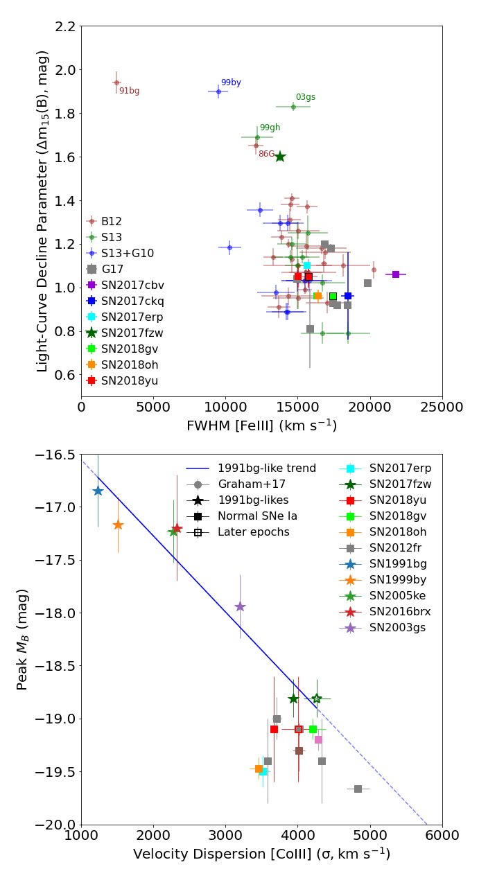
Figure 13: Top: The optical light-curve decline rate, $\Delta m_{15}(B)$, versus the full-width half-max (FWHM) of the [Fe iii] $\lambda$4700 Å feature in nebular-phase spectra (from a best-fit Gaussian function). Data are from Blondin et al. (2012, B13), Silverman et al. (2013, S13), Ganeshalingam et al. (2010, G10), Graham et al. (2017, G17), and this work (as labeled in the legend). The 91bg-like events are individually labeled. Bottom: The light-curve peak $B$-band brightness versus the velocity dispersion of the [Co iii] $\lambda$5890 Å feature (the standard deviation, $\sigma$). All velocity widths are from the “direct measure" method described in Section 3.4. SNe Ia that are 91bg-like or transitional are represented with 5-point stars, and normal SNe Ia with squares. Open symbols represent the later epochs for SNe Ia with two nebular-phase spectra (SNe 2017fzw and 2018yu). The solid blue line is a linear best-fit to the 91bg-like events, and is extended past SN 2017fzw as a dashed blue line to demonstrate the offset of normal SNe Ia from this trend.

The advantage of using parameters $\Delta m_{15}(B)$ and [Fe iii] FWHM for the top panel of Figure 13 is being able to easily include data from previous works, however, there are two main drawbacks. First, Garnavich et al. (2004) have shown that the light-curve decline rate $\Delta m_{15}(B)$ is not as well correlated with peak brightness for 91bg-likes as it is for normal SNe Ia. Second, the [Fe iii] feature is not isolated and has a significant flux contribution from neighboring features, and because some stable iron is formed in the explosion [Fe iii] is not as good a representative of the distribution of radioactive ⁵⁶Ni as [Co iii]. Thus, in the bottom panel of Figure 13 we plot the peak absolute $B$-band brightness as a function of the width of the [Co iii] $\lambda$5890 Å feature (using the direct measure method with psuedo-continuum subtraction; Section 3). The sample shown includes the same 91bg-like and transitional SNe Ia as in Figure 12, plus SN 2003gs (Silverman et al., 2012), along with the normal SNe Ia from Graham et al. (2017) and this work.

In the lower panel of Figure 13 we find that the 91bg-like and transitional events (all marked as five-point stars) show a clearer trend between peak brightness and [Co iii] line width, whereas the normal SNe Ia (squares) show no obvious trend. The best linear fit to the 91bg-like and transitional events is shown as a solid blue line, extended past SN 2017fzw (which was included in the fit) as a dashed blue line. The transitional SN Ia 2017fzw is unique in this sample because it sits within the region of $\Delta m_{15}(B)$ – $\sigma_{\rm[CoIII]}$ parameter space occupied by normal SN Ia events, yet also right on the best-fit line for transitional and 91bg-like events. This correlation between early- and late-time features for transitional SNe Ia like 2017fzw refutes our earlier hypothesis that the physical origins of transitional SNe Ia’s “91bg-likeness" might lay solely in the outer layers of the white dwarf.

5.4.4 The lack of a clear $M_{B}$ – [Co iii] line width correlation for normal SNe Ia

This trend prompts the question of why 91bg-like and transitional SNe Ia – fainter events that synthesized less ⁵⁶Ni – exhibit a clearer trend between ⁵⁶Ni mass (peak brightness) and nebular-phase velocity dispersion than normal SNe Ia. The ⁵⁶Ni mass represents the energy of the explosion, and the line width represents the kinetic energy of the ejecta material, and so these two parameters should be correlated for a sample of SNe Ia in which the ejecta mass is constant or has a shallow dependence on ⁵⁶Ni mass. Here we turn to Childress et al. (2015), which presented a method to estimate the ejecta mass from the flux of the nebular-phase [Co iii] $\lambda$ 5893 Å line for normal SN Ia events. They found that while ⁵⁶Ni mass exhibits a shallow correlation with ejecta mass for fainter, faster-declining SNe Ia, the ⁵⁶Ni mass was uncorrelated with ejecta mass for the normal and brighter, slowly-declining SNe Ia (Childress et al., 2015, their Figure 11). Although their analysis did not include SN 1991bg-like events, they are well-established to have low ejecta masses (e.g., Mazzali et al., 1997; Pakmor et al., 2010; Sullivan et al., 2011). Thus, a common and low ejecta mass could explain why the 91bg-like and transitional events exhibit a clear trend in Figure 13.

Furthermore, for normal SNe Ia, there are likely additional factors that influence the mass of ⁵⁶Ni synthesized in the explosion which are independent of the ejecta mass, such as the explosion mechanism itself – and additional factors which cause a scatter in the relation between peak brightness and ⁵⁶Ni (e.g., ejecta density or opacity). These factors could also explain why the normal events do not exhibit as clear a trend in Figure 13. As our collective sample of nebular-phase spectra for faint, transitional, and 91bg-like SNe Ia grows, we will be better able to establish and characterize such correlations and connect them to the underlying physical explosion mechanism, and provide better context for unique transitional events like SN 2017fzw.

5.5 SN 2018gv, a Spherically Symmetric SN Ia

5.5.1 Early-time SN 2018gv

SN 2018gv was discovered on 2018-01-15 by K. Itagaki in the outskirts of host galaxy NGC 2525 (Itagaki, 2018), a barred spiral galaxy at $z=0.00527$ (de Vaucouleurs et al., 1991) with a distance modulus of $\mu=31.1$ mag and a distance of $16.8$ Mpc (Tully et al., 2013). SN 2018gv was classified as a young, normal Type Ia supernova from an optical spectrum obtained with Keck Observatory on 2018-01-16 by Siebert et al. (2018, who also report the presence of C ii in this early spectrum), and from an optical spectrum obtained with the ESO New Technology Telescope on 2018-01-16 by Bufano et al. (2018).

Yang et al. (2020) present early-time data for SN 2018gv, showing that it reached a $B$-band peak of $12.6$ ($M_{B}=-19.1$) mag on 2018-01-31 and declined with $\Delta m_{15}(B)=0.96$ mag. Early optical spectropolarimetry obtained and analyzed by Yang et al. (2020) show low continuum polarization and moderate line polarization (for the photospheric absorption feature Si ii). They find that these observations indicate a high degree of spherical symmetry that is inconsistent with double-degenerate violent mergers (e.g., Pakmor et al. 2011), and consistent with both the double-detonation (e.g., Woosley & Weaver, 1994) and delayed detonation (e.g., Seitenzahl et al., 2013) models and predictions of their polarization signatures (Bulla et al., 2016). Yang et al. (2020) also demonstrate that SN 2018gv resembles SN 2011fe for the first $\sim 100$ days, and exhibits a low Si ii velocity gradient during the days after peak brightness ($33.3\pm 6.4$ $\rm km\ s^{-1}\ day^{-1}$), which agrees with the measurement from our early-time optical spectra of $29\pm 4$ $\rm km\ s^{-1}\ day^{-1}$ in Table 1.

A radio non-detection of SN 2018gv obtained on 2018-01-18.6 with the Australia Telescope Compact Array did not reveal any CSM, constraining the mass-loss rate of a non-degenerate companion star to $<1.3\times 10^{-8}$ $\rm M_{\odot}\ yr^{-1}$ (Ryder et al., 2018; Lundqvist et al., 2020). This radio non-detection for SN 2018gv rules out a symbiotic progenitor in which a white dwarf accretes material from a giant star, but cannot rule out progenitor systems containing, e.g., Roche Lobe overflow from a giant or main sequence star, or recurrent or quiescent novae (Lundqvist et al., 2020).

5.5.2 Late-time SN 2018gv

The fact that SN 2018gv appears to be a normal, SN 2011fe-like SN Ia with a high degree of spherical symmetry is well-supported by our nebular-phase spectrum. In Figure 2 we find a good match to the normal SN Ia 2011fe at similar phases, confirming that SN 2018gv is a typical SN Ia. A high degree of spherical symmetry would manifest as low velocity nebular features, and indeed we find that the [Fe ii]+[Ni ii] $\lambda$7200 Å feature of SN 2018gv exhibits an absolute velocity $<1000$ $\rm km\ s^{-1}$, which is among the lowest in our sample (Figure 6).

Radio non-detections ruled out a symbiotic system as the progenitor for SN 2018gv (Lundqvist et al., 2020), and so no nebular-phase H$\alpha$ is expected for SN 2018gv. Sand et al. (in prep.) perform a re-analysis of SN 2018gv’s nebular-phase spectrum which prioritizes the mitigation of host-galaxy H$\alpha$ emission, and find no evidence of an H$\alpha$ emission feature similar to expectations of swept-up material from a non-degenerate companion star (FWHM $\sim$1000 $\rm km\ s^{-1}$, velocity $\pm 1000$ $\rm km\ s^{-1}$), in agreement with expectations of the radio non-detection.

5.6 SN 2018oh, a SN Ia with Early-Time Kepler Photometry

5.6.1 Early-time SN 2018oh

SN 2018oh was discovered as ASASSN-18bt on 2018-02-04 with an apparent $V$-band magnitude of $15.15$ mag (Vega; Stanek 2018, and spectroscopically classified as a normal SN Ia about one week before peak brightness (Leadbeater, 2018). SN 2018oh resides in the central region of dwarf intermediate barred spiral galaxy UGC 04780 at $z=0.01098$ (Schneider et al., 1990).

Shappee et al. (2019) use time-series optical photometry of SN 2018oh from the Kepler Space Telescope (30-minute cadence) to show that the four days after first light exhibit a near linear rise, and that the pre-maximum light-curve is well fit by a double power law which suggests two independent luminosity sources. They demonstrate that the slower initial rise of SN 2018oh is not predicted by models of SN Ia ejecta impacting a non-degenerate companion, but is instead more compatible with the presence of ⁵⁶Ni in the outer layers of the ejecta. Shappee et al. (2019) also show that the optical data, along with X-ray nondetections from the Swift Space Telescope, together suggest an absence of any CSM as further evidence against the presence of a non-degenerate companion star.

Dimitriadis et al. (2019a) combine the Kepler data with their own ground-based optical photometry obtained within hours of the explosion, and show that the additional emission causing the early-time light curve bump was blue, with a blackbody temperature of $\sim 17500$ $\rm K$. They find that this evidence more strongly supports the hypothesis that this emission originates due to the impact of the SN Ia ejecta on a non-degenerate companion, and anticipate that the late-time spectra might thus exhibit H$\alpha$ emission. Dimitriadis et al. (2019a) make the point that aside from this fleeting evidence in the first four days, SN 2018oh appears to be a normal SN Ia – and thus that a much higher fraction of SN Ia might have non-degenerate companions than is generally thought.

Li et al. (2019) analyze the optical through near-infrared photometry (including the Kepler data) for the first 140 days after explosion. They report that SN 2018oh reached peak B-band luminosity on 2018 Feb 13.7 with an apparent brightness of $B=14.32\pm 0.01$ mag ($M_{B}=-19.47\pm 0.10$ mag), exhibited a decline rate of $\Delta m_{15}(B)=0.96\pm 0.03$ mag, and synthesized a nickel mass of $M_{\rm Ni}=0.55\pm 0.04$ $\rm M_{\odot}$. Könyves-Tóth et al. (2020) also analyze SN 2018oh’s light curve and report a slightly higher ⁵⁶Ni mass of $0.598\pm 0.059$ $\rm M_{\odot}$.

Li et al. (2019) present and analyze early-time optical spectroscopy of SN 2018oh and classify it as an LVG event. In addition, they show how C ii absorption is seen until 3 weeks after peak brightness, the latest such detection yet, indicating that unburned carbon exists deeper in the ejecta than for most SNe Ia. However, whether the carbon’s depth could be connected to mixing that brings ⁵⁶Ni to the surface, or whether abundance stratification or a low-metallicity progenitor allow the carbon feature to be visible for longer, would require additional modeling.

5.6.2 Late-time SN 2018oh

We find that the nebular-phase spectrum of SN 2018oh is quite similar to that of the normal SN Ia 2011fe (Figure 2), as expected. If the early-time blue component of SN 2018oh’s light curve, which was revealed by the Kepler photometry, is due to the ejecta interacting with CSM or a non-degenerate binary companion then we could expect to find H$\alpha$ emission in the nebular-phase spectrum. However, both Tucker et al. (2019) and Dimitriadis et al. (2019b) present and analyze late-time optical spectra for SN 2018oh, and place upper limits on hydrogen and helium emission which strongly indicate that SN 2018oh was a double-degenerate system of two white dwarf stars. Additionally, Tucker et al. (2020) find no evidence of stripped companion emission for SN 2018oh. This lack of late-time hydrogen or helium emission also agrees with the particular physical interpretation for SN 2018oh offered by Dimitriadis et al. (2019b), who show that the early-time blue bump could have originated from the interaction of SN Ia ejecta with a disk of material formed during the merger process of a white dwarf binary system. Sand et al. (in prep.) use the nebular spectra presented in this paper to place upper limits on the hydrogen emission as well. As with SN 2018gv, they re-process the spectra to account for host galaxy H$\alpha$ emission, and find no evidence of swept-up hydrogen from a non-degenerate companion star.

As previously discussed for SN 2017cbv in Section 5.1, mixing of ⁵⁶Ni into the outer layers is a potential alternative explanation for excess blue emission at early times, a physical trait which could manifest as broad emission features such as [Co iii] at nebular phases. However, SN 2018oh’s [Co iii] emission line does not appear to be broad, and was actually among the narrowest in our sample (Section 3.4, Tables 7 and 8 (Appendix A), and as seen in the bottom panel of Figure 13). The dense time-series of early-time optical spectra for SN 2018oh presented by Li et al. (2019) exhibited the latest ever detection of C ii, at three weeks after peak brightness. Such deep C ii could be related to mixing in the outer layers of the white dwarf, or could indicate a lower-metallicity progenitor in which there are less iron group elements to “smear out" the carbon feature (Li et al., 2019; Heringer et al., 2019). Figure 2 shows that SN 2018oh has a smaller [Ni ii] to [Fe ii] ratio than SN 2011fe, which would be consistent with a lower-metallicity progenitor in which less stable nickel is synthesized. However, as described in Section 4.4 we were unable to more robustly measure the Ni/Fe ratio for SN 2018oh from multi-component Gaussian fits.

5.7 SN 2018yu, a Normal SN Ia with a Near-Infrared Nebular Spectrum

5.7.1 Early-time SN 2018yu

SN 2018yu was discovered by the DLT40 survey as DLT18i on 2018-03-01 with an $r$-band apparent brightness of $17.6$ mag (Sand et al., 2018b), and within 24 hours was spectroscopically classified as a young SN Ia (Zhang & Wang, 2018). SN 2018yu is located in the outer disk of inclined spiral galaxy NGC 1888 at $z=0.00811$ (de Vaucouleurs et al., 1991), with a distance modulus of $32.85\pm 0.4$ mag and a distance of $37.1$ Mpc (Theureau et al., 2007).

The Las Cumbres optical photometry obtained around the time of peak brightness indicates a $B$-band decline rate of $\Delta m_{\rm 15}(B)\approx 1.05\pm 0.05$ mag and an intrinsic peak brightness of $M_{B}\approx-19.1\pm 0.5$ mag (Section 2.1). The light curve of SN 2018yu is consistent with a normal SN Ia on the Phillips relation (Phillips et al., 1999), and the early time spectra are consistent with a normal, LVG-type SN Ia.

5.7.2 Late-time SN 2018yu

SN 2018yu was a normal SN Ia at early times, and it appears to be normal at late times as well: its nebular-phase spectrum in the bottom panel of Figure 2 demonstrates that it is very similar to the prototypical SN 2011fe. Also, in Section 4 we show correlations between several measured parameters for the nebular-phase emission lines of the SNe Ia in our sample, and SN 2018yu always falls in the midst of the range of values. Sand et al. (in prep.) show that there is no signature of H$\alpha$ to indicate a non-degenerate companion for SN 2018yu, similar to the other SNe Ia in this sample. Additionally, Tucker et al. (2020) find no evidence of stripped companion emission for SN 2018yu.

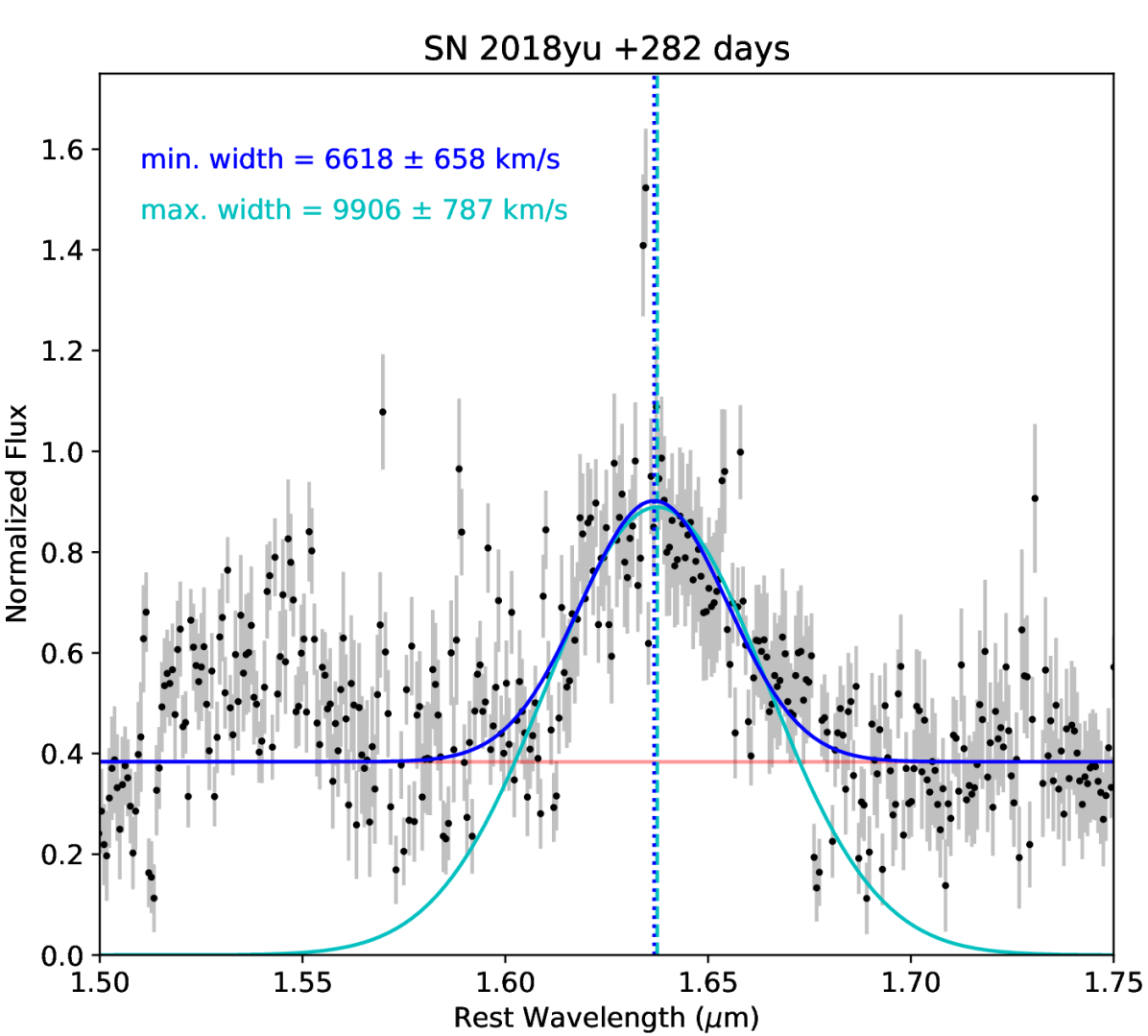
Figure 14: The [Fe ii] $\lambda$1.644 $\mu$m emission line in the +282 days NIR spectrum of SN 2018yu, obtained using Flamingos-2 on Gemini-South. As described in the text, the dark blue line is a single-Gaussian fit after subtracting a maximum flat continuum (red line; determined by the red side minimum of the [Fe ii] $\lambda$1.644 $\mu$m feature), which provides a minimum line width measurement The lighter teal line is a single-Gaussian fit assuming no underlying continuum, which provides the maximum possible line width. The minimum and maximum line widths provide constraints on the progenitor’s central density (Höflich, 2006; Diamond et al., 2015, 2018). Both fit methods also provide consistent line velocity measurements (dashed vertical lines) that agree with the [Fe ii] velocity measured in the optical.

To enrich our analysis of SN 2018yu, we include an NIR nebular-phase spectrum obtained with Flamingos-2 at Gemini-South Observatory at 282 days past peak brightness (Section 3.3), which is shown in Figure 14. One of the benefits of using NIR and optical spectra obtained at a similar nebular-phase epoch is that the [Fe ii] $\lambda$1.644 $\mu$m emission line is the strongest and most well-isolated iron feature in the NIR (Diamond et al., 2015, 2018), and originates from the same region of the SN ejecta as the [Fe ii] $\lambda$7155 Å line. This NIR emission line can be used to verify optical [Fe ii] line velocities and thus address line blending concerns in the 7200 Å feature. We measured the [Fe ii] $\lambda$1.644 $\mu$m line velocity with a least squares fit of a single Gaussian with a flat continuum, finding a velocity of $-1333\pm 385$ $\rm km\ s^{-1}$. The uncertainty was determined using a Monte Carlo approach: introducing random noise to the smoothed spectrum and calculating the dispersion of the line velocity from 5000 iterations. This NIR-derived iron velocity could be used to fix the iron velocity in our multi-Gaussian fits to the iron and nickel feature at $\lambda$7200 Å. However, it is not necessary to redo that fit for SN 2018yu because this NIR velocity is already in very good agreement with the result of that fit, $-1384.03\pm 71.11$ $\rm km\ s^{-1}$ (Section 4.4).

We also use the nebular-phase NIR spectrum of SN 2018yu to measure the width of the [Fe ii] $\lambda$1.644 $\mu$m line. Theoretical models suggest that carbon-oxygen white dwarfs with higher central densities will exhibit broader [Fe ii] $\lambda$1.644 $\mu$m features: a higher central density leads to a larger volume of stable material in the core, and the radioactive material – the source of the [Fe ii] emission – extends to higher velocities (e.g. Höflich et al., 2004; Motohara et al., 2006; Maeda et al., 2010b; Stritzinger et al., 2015). We follow the analysis method of Diamond et al. (2018) to measure the range of maximum and minimum possible line widths for the [Fe ii] $\lambda$1.644 $\mu$m line by assuming no continuum and a maximum flat continuum, respectively, as shown in Figure 14 and described in the figure’s caption. Compared to the models published in Diamond et al. (2018), our range of measured line widths for [Fe ii] $\lambda$1.644 $\mu$m for SN 2018yu corresponds to central densities of $\sim 0.5$ to $0.9\times 10^{9}$ $\rm g\ cm^{-3}$, which lies on the lower end of central densities included in these models. This could imply that the progenitor white dwarf of SN 2018yu experienced a high accretion rate from its companion, leading to a prompt explosion before it evolved to a higher central density. In this respect SN 2018yu is similar to SN 2014J, which Diamond et al. (2018) also suggest to have a low central density (and which, like SN 2018yu, exploded in the disk of a dusty host galaxy with a young stellar population).

6 Conclusions

We have presented nine new nebular-phase optical spectra from Gemini Observatory for seven nearby Type Ia supernovae with early-time optical photometric and spectroscopic monitoring from the Las Cumbres Observatory Global Supernova Project. The combination of early- and late-time data is essential for a comprehensive understanding of the explosion mechanisms and progenitor systems of SNe Ia, especially as they continue to be used as cosmological probes.

In this work we have shown that as our collection of nebular-phase observations continue to grow, analysis of ever larger samples continues to reveal how the temperature and ionization state of the nebula evolves with time; whether potential asymmetries in the explosion and nucleosynthetic material exist; consistency with various explosion models and WD progenitor masses; and the probability of WD-WD collisions or the presence of non-degenerate companion stars. Although most of the flux in the nebular spectrum is in smooth, broad emission features, our analysis has revealed that high signal-to-noise and high spectral resolution are beneficial for constraining the shape of the nebular features (i.e., fitting single- versus double- or multi-component features) and the presence of narrow hydrogen emission. Our analysis has also revealed the importance of obtaining phase-matched NIR nebular-phase spectra. Having the relatively isolated iron lines in the NIR would allow the iron line parameters to be held fixed when fitting the iron and nickel blended feature in the optical, and provide more accurate measures of the amount of stable nickel formed in the explosion.

We have also shown that analyses of individual SN Ia events remains a useful and enlightening exercise – especially for SNe Ia with unique observations or some kind of peculiarity at early times, such as the “blue bump" of SN 2017cbv, the depressed NUV flux of SN 2017erp, the spectropolarimetry of SN 2018gv, or the C ii of SN 2018oh. In particular, nebular-phase spectroscopy of subluminous, rapidly-evolving “91bg-like" and transitional SNe Ia such as SN 2017fzw remain rare and potentially high-impact. We recommend that the community continue to target subluminous, peculiar, and/or otherwise rare SNe Ia for nebular-phase follow-up in order to continue to advance our understanding of their progenitor systems and explosion mechanisms.

Data Availability

The raw optical spectra and calibration frames from Gemini Observatory are available via the Gemini Observatory Archive at archive.gemini.edu. The reduced spectra will be made available in the Weizmann Interactive Supernova Data Repository (WISeREP) at www.wiserep.org. The reduced data and derived measurements in this article will be shared on request to the corresponding author.

Appendix A Large Tables

SN Name	UT Date(a)	Phase	Instrument & Configuration(b)	Exposure
		[days]		Time [s]
2017cbv	2018-07-08	466	GMOS-S: B600,450,4x4	4x1200
	2018-07-11	469	GMOS-S: R400,750,4x4	4x1200
2017ckq	2018-04-12	369	GMOS-S: B600,450,4x4	6x1200
	2018-06-17	435	GMOS-S: R400,750,4x4	6x1200
2017erp	2018-03-16	259	GMOS-S: B600,520,2x2	4x300
	2018-03-22	265	GMOS-S: R400,750,2x2	2x300
	2018-04-12	286	GMOS-S: R400,750,2x2	4x300
2017fzw	2018-04-13	234	GMOS-S: B600,520,2x2	4x300
	2018-05-03	254	GMOS-S: R400,750,2x2	4x300
2018gv	2018-11-16	289	GMOS-S: B600,450,2x2	3x400
	2018-11-17	290	GMOS-S: R400,750,2x2	3x600
	2019-01-10	344	GMOS-S: B600,450,2x2	3x400
	2019-01-28	362	GMOS-S: R400,750,2x2	3x600
2018oh	2018-11-04	264	GMOS-N: B600,450,4x4	3x1200
	2018-12-07	297	GMOS-N: R400,750,4x4	3x1200
2018yu	2018-10-05	202	GMOS-S: B600,450,2x2	3x400
	2018-10-05	202	GMOS-S: R400,750,2x2	3x600
	2018-10-07	204	SALT: PG0900	2386
	2018-12-29	287	GMOS-S: B600,450,4x4	3x1200
	2019-01-06	295	GMOS-S: R400,750,4x4	4x1200

Table 6: Late-time optical spectroscopy for SNe Ia presented in this work. (a) Boldface dates and phases represent epochs, for which the R400 was flux-scaled and joined to the B600 spectrum. (b) Configurations for GMOS, the Gemini Multi-Object Spectrograph, list the grating (R400 or B600), the central wavelength in $\rm nm$, and the binning. All GMOS observations were done with the 0.75″ longslit.

Table 7: Directly measured parameters of nebular-phase emission lines.

SN Name	UT Date	Phase	Line	Velocity	FWHM	Integrated Flux
		[days]		[$\rm km\ s^{-1}$]	[$\rm km\ s^{-1}$]	[$\rm 10^{-15}\ erg\ s^{-1}\ cm^{-2}$]
2017cbv	2018-07-08	466	[FeIII]	$919\pm 138$	$9496\pm 324$	$2.545\pm 0.608$
2017ckq	2018-04-12	369	[FeIII]	$-348\pm 140$	$10855\pm 338$	$6.212\pm 1.175$
2017erp	2018-03-16	259	[FeIII]	$-1308\pm 41$	$11449\pm 97$	$35.383\pm 2.412$
2017erp	2018-03-16	259	[CoIII]	$-502\pm 102$	$8275\pm 222$	$3.116\pm 0.768$
2017fzw	2018-04-13	234	[FeIII]	$-715\pm 49$	$10504\pm 111$	$19.680\pm 1.715$
2017fzw	2018-04-13	234	[CoIII]	$738\pm 186$	$10032\pm 430$	$3.052\pm 1.217$
2018gv	2018-11-16	289	[FeIII]	$-1200\pm 29$	$12329\pm 72$	$55.357\pm 2.289$
2018gv	2018-11-16	289	[CoIII]	$-817\pm 180$	$9885\pm 445$	$4.416\pm 1.327$
2018gv	2019-01-10	344	[FeIII]	$-1078\pm 65$	$13082\pm 141$	$22.807\pm 1.953$
2018oh	2018-11-04	264	[FeIII]	$-1867\pm 119$	$12106\pm 283$	$18.198\pm 2.362$
2018oh	2018-11-04	264	[CoIII]	$-726\pm 119$	$8133\pm 289$	$2.010\pm 0.435$
2018yu	2018-10-05	202	[FeIII]	$-1573\pm 39$	$11927\pm 91$	$56.385\pm 4.225$
2018yu	2018-10-05	202	[CoIII]	$-563\pm 58$	$8418\pm 142$	$10.583\pm 1.366$
2018yu-	2018-10-07	204	[CoIII]	$-512\pm 41$	$8635\pm 99$	$4.207\pm 0.459$
2018yu	2018-12-29	287	[FeIII]	$-696\pm 42$	$11091\pm 94$	$22.663\pm 1.157$
2018yu	2018-12-29	287	[CoIII]	$-267\pm 223$	$9406\pm 540$	$1.547\pm 0.505$

Table 8: Gaussian fit parameters of nebular-phase emission lines.

SN Name	UT Date	Phase	Line	Velocity	FWHM	Integrated Flux
		[days]		[$\rm km\ s^{-1}$]	[$\rm km\ s^{-1}$]	[$\rm 10^{-15}\ erg\ s^{-1}\ cm^{-2}$]
2017cbv	2018-07-08	466	[FeIII]	$1541\pm 170$	$8188\pm 386$	$2.472\pm 0.077$
2017cbv	2018-07-08	466	[FeII]	$1163\pm 478$	$9472\pm 667$	$6.468\pm 0.729$
2017cbv	2018-07-08	466	[NiII]	$1325\pm 630$	$9250\pm 1024$	$4.471\pm 0.740$
2017ckq	2018-04-12	369	[FeIII]	$-384\pm 119$	$10372\pm 317$	$6.180\pm 0.125$
2017erp	2018-03-16	259	[FeIII]	$-1147\pm 35$	$10919\pm 90$	$35.566\pm 0.207$
2017erp	2018-03-16	259	[CoIII]	$-286\pm 92$	$7570\pm 221$	$3.190\pm 0.069$
2017erp	2018-03-16	259	[FeII]	$1210\pm 93$	$7885\pm 196$	$9.931\pm 0.252$
2017erp	2018-03-16	259	[NiII]	$1545\pm 138$	$7778\pm 263$	$6.961\pm 0.244$
2017fzw	2018-04-13	234	[FeIII]	$-581\pm 58$	$9714\pm 148$	$19.556\pm 0.203$
2017fzw	2018-04-13	234	[CoIII]	$1072\pm 172$	$8945\pm 443$	$3.030\pm 0.109$
2017fzw	2018-04-13	234	[FeII]	$2469\pm 131$	$10802\pm 343$	$6.341\pm 0.161$
2017fzw	2018-04-13	234	[NiII]	$2986\pm 86$	$5252\pm 170$	$2.929\pm 0.129$
2018gv	2018-11-16	289	[FeIII]	$-1181\pm 26$	$11519\pm 77$	$55.748\pm 0.234$
2018gv	2018-11-16	289	[CoIII]	$-728\pm 141$	$9730\pm 334$	$4.459\pm 0.113$
2018gv	2018-11-16	289	[FeII]	$-761\pm 46$	$7028\pm 124$	$8.704\pm 0.131$
2018gv	2018-11-16	289	[NiII]	$-214\pm 82$	$7280\pm 229$	$5.087\pm 0.128$
2018gv	2019-01-10	344	[FeIII]	$-940\pm 46$	$12108\pm 124$	$22.923\pm 0.157$
2018gv	2019-01-10	344	[FeII]	$-874\pm 154$	$7075\pm 326$	$5.121\pm 0.293$
2018gv	2019-01-10	344	[NiII]	$-416\pm 259$	$9013\pm 565$	$4.897\pm 0.281$
2018oh	2018-11-04	264	[FeIII]	$-1678\pm 90$	$12165\pm 235$	$18.188\pm 0.238$
2018oh	2018-11-04	264	[CoIII]	$-999\pm 97$	$8039\pm 247$	$1.994\pm 0.047$
2018oh	2018-11-04	264	[FeII]	$-1489\pm 87$	$6212\pm 256$	$3.620\pm 0.143$
2018oh	2018-11-04	264	[NiII]	$-1546\pm 219$	$7445\pm 536$	$2.234\pm 0.141$
2018yu	2018-10-05	202	[FeIII]	$-1592\pm 38$	$10823\pm 108$	$57.145\pm 0.397$
2018yu	2018-10-05	202	[CoIII]	$-600\pm 53$	$7957\pm 137$	$10.601\pm 0.124$
2018yu	2018-10-05	202	[FeII]	$-924\pm 60$	$6511\pm 134$	$7.872\pm 0.166$
2018yu	2018-10-05	202	[NiII]	$-1154\pm 121$	$7857\pm 269$	$5.308\pm 0.174$
2018yu	2018-10-07	204	[CoIII]	$-391\pm 39$	$8037\pm 106$	$4.239\pm 0.039$
2018yu	2018-10-07	204	[FeII]	$-992\pm 67$	$6340\pm 129$	$4.059\pm 0.097$
2018yu	2018-10-07	204	[NiII]	$-1384\pm 136$	$8001\pm 314$	$2.857\pm 0.098$
2018yu	2018-12-29	287	[FeIII]	$-653\pm 38$	$10842\pm 106$	$23.012\pm 0.140$
2018yu	2018-12-29	287	[CoIII]	$-344\pm 194$	$8540\pm 624$	$1.571\pm 0.071$
2018yu	2018-12-29	287	[FeII]	$-880\pm 91$	$6631\pm 264$	$4.315\pm 0.167$
2018yu	2018-12-29	287	[NiII]	$-780\pm 166$	$7994\pm 404$	$3.585\pm 0.163$

References

- Arnett (1982) Arnett W. D., 1982, ApJ, 253, 785
- Arnett & Livne (1994) Arnett D., Livne E., 1994, ApJ, 427, 314
- Ashall et al. (2016) Ashall C., Mazzali P. A., Pian E., James P. A., 2016, MNRAS, 463, 1891
- Benetti et al. (2005) Benetti S., et al., 2005, ApJ, 623, 1011
- Bertin & Arnouts (1996) Bertin E., Arnouts S., 1996, A&AS, 117, 393
- Black et al. (2016) Black C. S., Fesen R. A., Parrent J. T., 2016, MNRAS, 462, 649
- Blondin et al. (2012) Blondin S., et al., 2012, AJ, 143, 126
- Blondin et al. (2017) Blondin S., Dessart L., Hillier D. J., Khokhlov A. M., 2017, MNRAS, 470, 157
- Blondin et al. (2021) Blondin S., Bravo E., Timmes F., Dessart L., Hillier D. J., 2021, arXiv e-prints, p. arXiv:2109.13840
- Botyánszki & Kasen (2017) Botyánszki J., Kasen D., 2017, ApJ, 845, 176
- Botyánszki et al. (2018) Botyánszki J., Kasen D., Plewa T., 2018, ApJ, 852, L6
- Brown et al. (2013) Brown T. M., et al., 2013, PASP, 125, 1031
- Brown et al. (2019) Brown P. J., et al., 2019, ApJ, 877, 152
- Bufano et al. (2018) Bufano F., et al., 2018, The Astronomer’s Telegram, 11177, 1
- Bulla et al. (2016) Bulla M., et al., 2016, MNRAS, 462, 1039
- Burns et al. (2020) Burns C. R., et al., 2020, ApJ, 895, 118
- Cappellaro et al. (2001) Cappellaro E., et al., 2001, ApJ, 549, L215
- Cartier et al. (2017) Cartier R., et al., 2017, MNRAS, 464, 4476
- Childress et al. (2015) Childress M. J., et al., 2015, MNRAS, 454, 3816
- Cristiani et al. (1992) Cristiani S., et al., 1992, A&A, 259, 63
- Dessart et al. (2014) Dessart L., Hillier D. J., Blondin S., Khokhlov A., 2014, MNRAS, 439, 3114
- Dessart et al. (2020) Dessart L., Leonard D. C., Prieto J. L., 2020, A&A, 638, A80
- Diamond et al. (2015) Diamond T. R., Hoeflich P., Gerardy C. L., 2015, ApJ, 806, 107
- Diamond et al. (2018) Diamond T. R., et al., 2018, ApJ, 861, 119
- Dimitriadis et al. (2017) Dimitriadis G., et al., 2017, MNRAS, 468, 3798