Inferring $S_{8}(z)$ and $\gamma(z)$ with cosmic growth rate measurements using machine learning

Abstract

Measurements of the cosmological parameter $S_{8}$ provided by cosmic microwave background and large scale structure data reveal some tension between them, suggesting that the clustering features of matter in these early and late cosmological tracers could be different. In this work, we use a supervised learning method designed to solve Bayesian approach to regression, known as Gaussian Processes regression, to quantify the cosmic evolution of $S_{8}$ up to $z\sim 1.5$. For this, we propose a novel approach to find firstly the evolution of the function $\sigma_{8}(z)$, then we find the function $S_{8}(z)$. As a sub-product we obtain a minimal cosmological model-dependent $\sigma_{8}(z=0)$ and $S_{8}(z=0)$ estimates. We select independent data measurements of the growth rate $f(z)$ and of $[f\sigma_{8}](z)$ according to criteria of non-correlated data, then we perform the Gaussian reconstruction of these data sets to obtain the cosmic evolution of $\sigma_{8}(z)$, $S_{8}(z)$, and the growth index $\gamma(z)$. Our statistical analyses show that $S_{8}(z)$ is compatible with Planck $\Lambda$CDM cosmology; when evaluated at the present time we find $\sigma_{8}(z=0)=0.766\pm 0.116$ and $S_{8}(z=0)=0.732\pm 0.115$. Applying our methodology to the growth index, we find $\gamma(z=0)=0.465\pm 0.140$. Moreover, we compare our results with others recently obtained in the literature. In none of these functions, i.e. $\sigma_{8}(z)$, $S_{8}(z)$, and $\gamma(z)$, do we find significant deviations from the standard cosmology predictions.

1 Introduction

The way how the matter clusters throughout the universe evolution is one of the critical probes to judge whether the concordance model $\Lambda$CDM is, in fact, the standard model of cosmology. In front of this scenario, accurate measurements of $f(z)$, the growth rate of cosmic structures, and of $\sigma_{8}(z)$, the variance of the matter fluctuations at the scale of 8 Mpc$/h$, are important scientific targets of current and future large astronomical surveys (Pezzotta17, ; Aubert20, ; Bautista21, ).

The growth rate, $f$, represents a measure of the matter clustering evolution from the primordial density fluctuations to the large-scale structures observed today, as such it behaves differently in $\Lambda$CDM-type models, based on the theory of general relativity (GR), and in alternative models of cosmology, based on modified gravity theories. On the other hand, $\sigma_{8,0}\equiv\sigma_{8}(z=0)$ can be obtained using the cosmic microwave background (CMB) data, where it scales the overall amplitude of the measured angular power spectrum (Planck20, ).

The growth rate of cosmic structures is defined as $f(a)\equiv d\ln D(a)/d\ln a$, where $D=D(a)$ is the linear growth function, and $a$ is the scale factor in the Robertson-Walker metric, based on GR theory. A direct measurement of $f$ applying the above relationship to a given data set does not work because the cosmological observable is the density contrast and not the growth function $D(a)$ (Avila22, ). However, it is possible to obtain indirect measurements of $f$ if one can measure the velocity scale parameter $\beta\equiv f/b$, and one knows the linear bias $b$ of the cosmological tracer used in the measurement of $\beta$ (Bilicki11, ; Boruah20, ; Said20, ; Avila21, ). Additionally, the most common approach to quantify the clustering evolution of cosmic structures is in the form of their product , $[f\sigma_{8}](z)$, through the analyses of the Redshift Space Distortions (RSD) (Perenon20, ), that is, studying the distortions in the two-point correlation function (2PCF) caused by the Doppler effect of galaxy peculiar velocities, associated with the gravitational growth of inhomogeneities (Kaiser87, ) (for other applications of the 2PCF in matter clustering analyses see, e.g., Avila18, ; Avila19, ; Pandey20, ; Pandey21b, ; deCarvalho20, ; deCarvalho21, ).

Efforts done in recent years have provided measurements of both quantities: $f\sigma_{8}$ and $f$, at various redshifts and through the analyses of a diversity of cosmological tracers, including luminous red galaxies, blue galaxies, voids, and quasars. We shall explore these data to find, as robust as possible, a measurement of $\sigma_{8}(z)$ and $S_{8}(z)$, quantities that has been reported to be in some tension when comparing the measurements from the last Planck CMB data release (Planck20, ) with the analyses from several large-scale structure surveys (Amico20, ; Philcox_2020, ; Garcia21, ; Valentino_2021_S8, ; perivolaropoulos2021challenges, ; Huang21, ; Nunes2021S8, ).

The main objective of our analyses is to break the degeneracy in the product function $[f\sigma_{8}](z)$ using the cosmic growth rate data $f(z)$, to know the evolution of the functions $\sigma_{8}(z)$ and $S_{8}(z)$. In turn, the knowledge of $\sigma_{8}(z)$ provides its value at $z=0$, $\sigma_{8,0}$, an interesting outcome of these analyses considering the current $\sigma_{8}$-tension reported in the literature (Valentino_2021_S8, ; perivolaropoulos2021challenges, ; Nunes2021S8, ). Our approach consists of using the Gaussian processes tool to reconstruct the functions $[f\sigma_{8}](z)$ and $f(z)$, using for this task two data sets: 20 measurements of $[f\sigma_{8}](z)$ and 11 measurements of $f(z)$, respectively. The reconstructed functions $[f\sigma_{8}]^{\mbox{\sc\,gp}}(z)$ and $f^{\mbox{\sc\,gp}}(z)$ allow us to know the function $\sigma_{8}(z)$, as described in the next section.

This work is organized as follows. In section 2 we review the main equations of the linear theory of matter perturbations. In section 3 we present the data sets and describe the statistical methodology used in our analyses. Section 4 we report our main results and discussions. We draw our concluding remarks in Section 5.

2 Theory

On sub-horizon scales, in the linear regime, and assuming that dark energy does not cluster, the evolution equation for the growth function is given by

$$\frac{df(a)}{d\ln a}+f^{2}+\left(2+\frac{1}{2}\frac{d\ln H(a)^{2}}{d\ln a}\right)f-\frac{3}{2}\Omega_{m}(a)=0\,,$$ (1)

where $\Omega_{m}(a)\equiv\Omega_{m,0}\,a^{-3}H_{0}^{2}/H(a)^{2}$, with $\Omega_{m,0}\equiv\Omega_{m}(z=0)$ the matter density parameter today, and $H(a)$ is the Hubble rate as a function of the scale factor, $a$. A good approximation for $f(z)$ is given by (Wang98, ; Amendola04, ; Linder05, )

$$f(z)\simeq\Omega_{m}^{\gamma}(z)\,,$$ (2)

where $\gamma$ is termed the growth index. For dark energy models within GR theory $\gamma$ is considered a constant with approximate value $\gamma\simeq 3(\omega-1)/(6\omega-5)$ (Linder07, ). In the $\Lambda$CDM model, where $\omega=-1$, one has $\gamma=6/11\simeq 0.55$. However, in alternative cosmological scenarios the growth index can indeed assume distinct functional forms beyond the constant value (Linder07, ; Batista14, ). In fact, from equation (2) one can define,

$$\gamma(z)\equiv\frac{\ln f(z)}{\ln\Omega_{m}(z)}\,,$$ (3)

a more general definition for $\gamma$.

The mass variance of the matter clustering is given by

$$\sigma^{2}_{R}(z)=\frac{1}{2\pi^{2}}\int_{0}^{\infty}\!P(k,z)W_{R}^{2}(k)dk\,,$$ (4)

where $P(k,z)$ is the matter power spectrum and $W_{R}(k)$ is the window function with $R$ symbolizing a physical scale. The matter power spectrum can be written as

$$P(k,z)=\left[\frac{D(z)}{D(z=0)}\right]^{2}T^{2}(k)P(k,z=0)\,,$$ (5)

where $T^{2}(k)$ is the transfer function. One can write the equation (4) as

$$\sigma_{R}^{2}(z)=D^{2}(z)\sigma_{R}^{2}(z=0)\,,$$ (6)

assuming the normalization $D(z=0)=1$ for the linear growth function $D(z)$ (Marques20, ).

From the analyses of diverse cosmological tracers it is common to perform the measurements at scales of $R=8$ Mpc$/h$, that is, $\sigma_{8,0}\equiv\sigma_{8}(z=0)$. Thus, for the scale of $8$ Mpc$/h$ one has

$$\sigma_{8}(z)=D(z)\,\sigma_{8,0}\,.$$ (7)

Then, the product $[f\sigma_{8}](z)$ can be written as

$$[f\sigma_{8}](z)=-\,\sigma_{8,0}\,(1+z)\,\frac{dD(z)}{dz}\,,$$ (8)

which directly measures the matter density perturbation rate.

For the purpose of our analyses, one can obtain the function $\sigma_{8}(z)$ as the quotient of the functions

$$\sigma_{8}^{\text{q}}(z)\equiv\frac{[f\sigma_{8}]^{\mbox{\sc\,gp}}(z)}{f^{\mbox{\sc\,gp}}(z)}\,,$$ (9)

where $f^{\mbox{\sc\,gp}}(z)$ and $[f\sigma_{8}]^{\mbox{\sc\,gp}}(z)$ were reconstructed using Gaussian Processes from measurements of $f(z)$ and $[f\sigma_{8}](z)$, respectively. The superscript ‘q’ in $\sigma_{8}^{\text{q}}$ is used to indicate the quotient shown in equation (9).

Once we obtain the function $\sigma_{8}^{\text{q}}(z)$, we shall obtain the function $S_{8}(z)$ through

$$S_{8}(z)\equiv\sigma_{8}^{\text{q}}(z)\left(\frac{\Omega_{m}(z)}{0.30}\right)^{1/2}\,.$$ (10)

3 Data set and Methodology

In this section we present the $f(z)$ and $[f\sigma_{8}](z)$ data used to reconstruct first the $f^{\mbox{\sc\,gp}}(z)$ and $[f\sigma_{8}]^{\mbox{\sc\,gp}}(z)$ functions, then used to infer the cosmic evolution of the $\sigma_{8}(z)$ and $S_{8}(z)$ functions. In addition to these data, we use a set of $E(z)$ measurements performed by Ez2018a , in the redshift interval $z\in[0.0,1.5]$, to reconstruct the $\gamma(z)$ function defined in equation (3).

3.1 The $f(z)$ data

The literature reports diverse compilations of measurements of the growth rate of cosmic structures, $[f\sigma_{8}](z)$ (see, e.g. Basilakos12, ; Nunes16, ; Bessa21, ), which we update here. Our compilation of $f(z)$ data, shown in table 1, follows these criteria:

(i) We consider $f(z)$ data obtained from uncorrelated redshift bins when the measurements concern the same cosmological tracer, and data from possibly correlated redshift bins when different cosmological tracers were analysed.

(ii) We consider only data with a direct measurement of $f$, and not measurements of $f\sigma_{8}$ that use a fiducial cosmological model to eliminate the $\sigma_{8}$ dependence.

(iii) We consider the latest measurement of $f$ when the same survey collaboration performed two or more measurements corresponding to diverse data releases.

Table 1: Data compilation of 11 $f(z)$ measurements; see section 3 for details.

Survey	$z$	$f$	Reference	Cosmological tracer
ALFALFA	0.013	$0.56\pm 0.07$	Avila21	HI extragalactic sources
2dFGRS	0.15	$0.49\pm 0.14$	Hawkins03 ; Guzzo08	galaxies
GAMA	0.18	$0.49\pm 0.12$	Blake13	multiple-tracer: blue & red gals.
WiggleZ	0.22	$0.60\pm 0.10$	Blake11	galaxies
SDSS	0.35	$0.70\pm 0.18$	Tegmark06	luminous red galaxies (LRG)
GAMA	0.38	$0.66\pm 0.09$	Blake13	multiple-tracer: blue & red gals.
WiggleZ	0.41	$0.70\pm 0.07$	Blake11	galaxies
2SLAQ	0.55	$0.75\pm 0.18$	Ross07	LRG & quasars
WiggleZ	0.60	$0.73\pm 0.07$	Blake11	galaxies
VIMOS-VLT Deep Survey	0.77	$0.91\pm 0.36$	Guzzo08	faint galaxies
2QZ & 2SLAQ	1.40	$0.90\pm 0.24$	DaAngela08	quasars

3.2 The $[f\sigma_{8}](z)$ data

In table 2 we present our compilation of $f\sigma_{8}$ data. The criteria for selecting these data are:

(i) We consider $[f\sigma_{8}](z)$ data obtained from uncorrelated redshift bins when the measurements concern the same cosmological tracer, and data from possibly correlated redshift bins when different cosmological tracers were analysed.

(ii) We consider direct measurements of $f\sigma_{8}$.

(iii) We consider the latest measurement of $f\sigma_{8}$ when the same survey collaboration performed two or more measurements corresponding to diverse data releases.

Table 2: Data compilation of 20 $[f\sigma_{8}](z)$ measurements; see section 3 for details.

Survey	$z$	$f\sigma_{8}$	Reference	Cosmological tracer
SnIa+IRAS	0.02	$0.398\pm 0.065$	Turnbull12	SNIa + galaxies
6dFGS	0.025	$0.39\pm 0.11$	Achitouv17	voids
6dFGS	0.067	$0.423\pm 0.055$	Beutler12	galaxies
SDSS-veloc	0.10	$0.37\pm 0.13$	Feix15	DR7 galaxies
SDSS-IV	0.15	$0.53\pm 0.16$	Alam17	eBOSS DR16 MGS
BOSS-LOWZ	0.32	$0.384\pm 0.095$	Sanchez14	DR10, DR11
SDSS-IV	0.38	$0.497\pm 0.045$	Alam17	eBOSS DR16 galaxies
WiggleZ	0.44	$0.413\pm 0.080$	Blake12	bright emission-line galaxies
CMASS-BOSS	0.57	$0.453\pm 0.022$	Nadathur19	DR12 voids+galaxies
SDSS-CMASS	0.59	$0.488\pm 0.060$	Chuang16	DR12
SDSS-IV	0.70	$0.473\pm 0.041$	Alam17	eBOSS DR16 LRG
WiggleZ	0.73	$0.437\pm 0.072$	Blake12	bright emission-line galaxies
SDSS-IV	0.74	$0.50\pm 0.11$	Aubert20	eBOSS DR16 voids
VIPERS v7	0.76	$0.440\pm 0.040$	Wilson16	galaxies
SDSS-IV	0.85	$0.52\pm 0.10$	Aubert20	eBOSS DR16 voids
SDSS-IV	0.978	$0.379\pm 0.176$	Zhao19	eBOSS DR14 quasars
VIPERS v7	1.05	$0.280\pm 0.080$	Wilson16	galaxies
FastSound	1.40	$0.482\pm 0.116$	Okumura16	ELG
SDSS-IV	1.48	$0.30\pm 0.13$	Aubert20	eBOSS DR16 voids
SDSS-IV	1.944	$0.364\pm 0.106$	Zhao19	eBOSS DR14 quasars

  

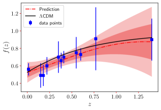
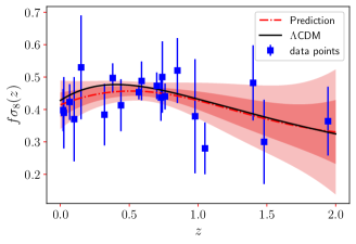
Figure 1: Left panel: Growth rate reconstruction $f^{\mbox{\sc gp}}(z)$ from table 1. Right panel: The reconstruction of $[f\sigma_{8}]^{\mbox{\sc gp}}(z)$ function using the sample in table 2. In both plots the shaded areas represent the $1\sigma$ and $2\sigma$ CL regions.

3.3 Gaussian Processes Regression

To extract maximum cosmological information from a given data set, as for instance the $f$ and $f\sigma_{8}$ data listed in Tables 1 and 2, we perform a Gaussian Processes Regression (GP), obtaining in this way smooth curves for the functions $f^{\mbox{\sc gp}}(z)$ and $[f\sigma_{8}]^{\mbox{\sc gp}}(z)$ according to the approach described in section 2. Both reconstructed functions are then used to obtain the cosmic evolution of $\sigma_{8}^{\text{q}}(z)$ and $S_{8}(z)$.

The GP consists of generic supervised learning method designed to solve regression and probabilistic classification problems, where we can interpolate the observations and compute empirical confidence intervals and a prediction in some region of interest (Rasmussen, ). In the cosmological context, GP techniques has been used to reconstruct cosmological parameters, like the dark energy equation of state, $w(z)$, the expansion rate of the universe, the cosmic growth rate, and other cosmological functions (see, e.g., Seikel12 ; Shafieloo12 ; Javier16 ; Javier17 ; Zhang18 ; Marques19 ; Renzi20 ; Benisty20 ; Bonilla21a ; Bonilla:2020wbn ; Colgain21 ; Sun21 ; renzi2021resilience ; bengaly2021null ; Escamilla-Rivera2021 ; Dhawan2021 ; Mukherjee2021 ; Keeley2021 ; Huillier2020 ; Avila22 ; ruizzapatero2022modelindependent for a short list of references).

The main advantage in this procedure is that it is able to make a non-parametric inference using only a few physical considerations and minimal cosmological assumptions. Our aim is to reconstruct a function $F(x)$ from a set of its measured values $F(x_{i})\pm\sigma_{i}$, for different values $\{x_{i}\}$ of the variable $x$. It assumes that the value of the function at any point $x_{i}$ follows a Gaussian distribution. The value of the function at $x_{i}$ is correlated with the value at other point $x_{i}^{\prime}$. Thus, a GP is defined as

$$F(x_{i})=\mathcal{GP}(\mu(x_{i}),\textrm{cov}[F(x_{i}),F(x_{i})])\,,$$ (11)

where $\mu(x_{i})$ and $\textrm{cov}[F(x_{i}),F(x_{i})]$ are the mean and the variance of the variable at $x_{i}$, respectively. For the reconstruction of the function $F(x_{i})$, the covariance between the values of this function at different positions $x_{i}$ can be modeled as

$$\textrm{cov}[F(x),F(x^{\prime})]=k(x,x^{\prime})\,,$$ (12)

where $k(x,x^{\prime})$ is known as the kernel function. The kernel choice is often very crucial to obtain good results regarding the reconstruction of the function $F(x)$.

The kernel most commonly used is the standard Gaussian Squared-Exponential (SE) approach, defined as

$$k_{\text{SE}}(x,x^{\prime})=\sigma_{F}^{2}\exp\left(-\frac{|x-x^{\prime}|^{2}}{2l^{2}}\right)\,,$$ (13)

where $\sigma_{F}^{2}$ is the signal variance, which controls the strength of the correlation of the function $F$, and $l$ is the length scale that determines the capacity to model the main characteristics (global and local) of $F$ in the evaluation region ($l$ measures the coherence length of the correlation in $x$). These two parameters are often called hyper-parameters.

However, given the irregular pattern noticed in our data sets (observe the blue squares representing the $f(z)$ and $[f\sigma_{8}](z)$ data shown in the plots of figure 1), a more general kernel is suitable for the GP analyses, namely the Rational Quadratic kernel (RQ), defined as (Rasmussen, )

$$k_{\text{RQ}}(x,x^{\prime})=\left(1+\frac{|x-x^{\prime}|^{2}}{2\alpha l^{2}}\right)^{-\alpha}\,,$$ (14)

where $\alpha$ is the scale mixture parameter. This kernel can be seen as an infinite sum of SE kernels with different characteristic length-scales.

Beside the choice of the kernel, the length scale bounds also have an influence in the results, as discussed in Sun21 ; Perenon21 . For data showing irregular pattern behavior, as the data we are considering for analyses, a more restrictive bounds for the hyper-parameters are necessary. To reconstruct the function $[f\sigma_{8}](z)$ correctly, our choice for the length scale bound corresponds to the redshift interval of the sample. For the $f\sigma_{8}$ sample, for instance, we fix the priors $0.1\leq l\leq 2$ and $0.1\leq\alpha\leq 2$.

It is worth mentioning that the choice of the kernel and the length scale parameters, $l$ and $\alpha$, were delicate steps for a robust GP reconstruction of the function $\gamma(z)$ from the $[f\sigma_{8}](z)$ data sample. However, the reconstructed functions $\sigma_{8}^{\text{q}}(z)$ and $S_{8}(z)$ were obtained robustly against those particular choices, and this is also true for the $\gamma(z)$ function reconstructed using the $f(z)$ and $E(z)$ data.

4 Results and Discussions

The left panel of figure 1 shows the $f(z)$ reconstruction at $1\sigma$ and $2\sigma$ confidence levels (CL) in the redshift range $z\in[0.0,1.4]$, and the blue squares are the data points from table 1. The dash-dot line is the prediction obtained from the GP using the RQ kernel. When evaluated at the present time, we find $f(z=0)=0.526\pm 0.060$ at $1\sigma$ CL. In the right panel of figure 1 we quantify the same statistical information, but assuming our $[f\sigma_{8}](z)$ data sample. When evaluated at the present time, $z=0$, we find $f\sigma_{8}(z=0)=0.414\pm 0.038$ at 1$\sigma$ CL. In both panels, the black solid line represents the $\Lambda$CDM prediction with the Planck-CMB best fit values (Aghanim:2018eyx, ). One can notice that the model-independent obtained here from both data samples, tables 1 and 2, predicts a smaller amplitude in comparison with $\Lambda$CDM model, but globally compatible within $2\sigma$ uncertainties.

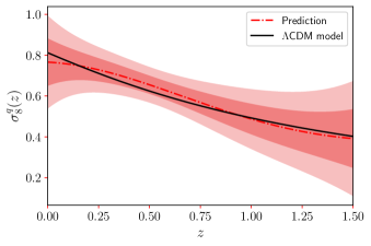
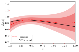
Figure 2: Left panel: Reconstruction of the function $\sigma_{8}^{\text{q}}(z)$ (the letter q to remember its origin: the quotient of two continuous functions) at $1\sigma$ and $2\sigma$ CL obtained from our $[f\sigma_{8}](z)$ and $f(z)$ data sample. The dot-dashed line represents the prediction from the data. Right panel: Same as in left panel, but for the $S_{8}(z)$ function. The black line represents the prediction from the $\Lambda$CDM model considering the Planck-CMB cosmological parameters.

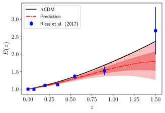
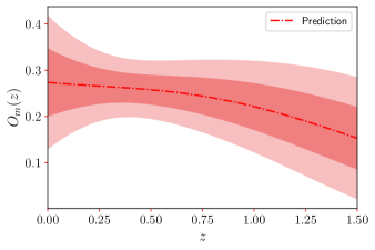
Figure 3: Left panel: Reconstruction of the $E(z)$ function from the Pantheon sample. Right panel: Reconstruction of the $O_{m}(z)$ diagnostic test function from the Pantheon sample. The black line represents $\Lambda$CDM model from Planck-CMB values.

Figure 2 on the left panel shows the function $\sigma_{8}^{\text{q}}(z)$ obtained through the methodology described in section 2. When evaluated at the present time, we find $\sigma_{8,0}^{\text{q}}=0.766\pm 0.116$ at 1$\sigma$ CL. On the right panel of figure 2 we show the function $S_{8}$ obtained using $\sigma_{8}^{\text{q}}(z)$ according to equation (10). Here one notices that for such a procedure we need infer also a reconstruction process for the function $\Omega_{m}(z)$. For this, in the context of the standard framework, we can use the $O_{m}(z)$ diagnostic function (Om2008, )

$$O_{m}(z)=\frac{E^{2}(z)-1}{(1+z)^{3}-1}\,.$$ (15)

If the expansion history $E(z)$ is driven by the standard $\Lambda$CDM model with null spatial curvature, then the function $O_{m}(z)$ is proportional to the matter density $\Omega_{m}(z)$. To reconstruct the $\Omega_{m}(z)$ function in minimal model assumptions, let us use the Supernovae Type Ia data from the Pantheon sample (Scolnic:2017caz, ). As is well known, the Supernovae Type Ia traditionally have been one of the most important astrophysical tools in establishing the so-called standard cosmological model. For the present analyses, we use the Pantheon compilation, which consists of 1048 SNIa distributed in the range $0.01<z<2.3$ (Scolnic:2017caz, ). With the hypothesis of a spatially flat Universe, the full sample of Pantheon can be binned into six model independent $E(z)$ data points (Ez2018a, ). We study the six data points reported by Ez2018b in the form of $E(z)$, including theoretical and statistical considerations made by the authors there for its implementation. Under these considerations, we find $\Omega_{m,0}=0.274\pm 0.073$ at $1\sigma$ CL. Note that this estimate is model-independent. Then, we reconstruct the evolution of the matter density in a model-independent way, by applying again the Pantheon sample on the definition $\Omega_{m}(z)\equiv\Omega_{m,0}(1+z)^{3}/E^{2}(z)$. Figure 3 on the left panel shows the robust reconstruction for the $E(z)$ function and on the right panel for the $O_{m}(z)$ diagnostic function. After these steps, we can infer the reconstruction for the $S_{8}$ function as a function of redshift (right panel in figure 2). When evaluated at the present time, we find $S_{8}(z=0)=0.732\pm 0.115$ at $1\sigma$ CL.

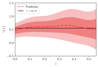
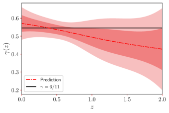
Figure 4: Left panel: Reconstruction of the $\gamma(z)$ function with the $f(z)$ sample. Right panel: Reconstruction of the $\gamma(z)$ function with the $f\sigma_{8}$ sample.

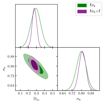
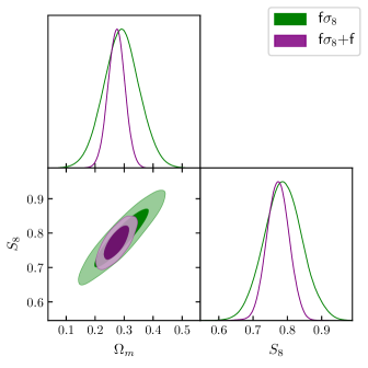
Figure 5: 1D and 2D posterior distributions for $[f\sigma_{8}](z)$ and $[f\sigma_{8}](z)$ + $f(z)$ data at $1\sigma$ and $2\sigma$ CL. Left panel: Contour diagram on the plane $\Omega_{m}-\sigma_{8}$. Right panel: Contour diagram on the plane $\Omega_{m}-S_{8}$.

Within the context of the $\Lambda$CDM model, CMB temperature fluctuations measurements from Planck and ACT+WMAP indicate $S_{8}$ values of $0.834\pm 0.016$ (Aghanim:2018eyx, ) and $0.840\pm 0.030$ (Aiola:2020azj, ), respectively. On the other hand, the value of $S_{8}$ inferred by a host of weak lensing and galaxy clustering measurements is typically lower than the CMB-inferred values, ranging between $0.703$ to $0.782$: examples of surveys reporting lower values of $S_{8}$ include CFHTLenS (Joudaki:2016mvz, ), KiDS-450 (Joudaki:2016kym, ), KiDS-450+2dFLenS (Joudaki:2017zdt, ), KiDS+VIKING-450 (KV450) (Hildebrandt:2018yau, ), DES-Y1 (Troxel:2017xyo, ), KV450+BOSS (Troster:2019ean, ), KV450+DES-Y1 (Joudaki:2019pmv, ; Asgari:2019fkq, ), a re-analysis of the BOSS galaxy power spectrum (Ivanov:2019pdj, ), KiDS-1000 (Asgari:2020wuj, ), and KiDS-1000+BOSS+2dFLenS (Heymans:2020ghw, ). Planck Sunyaev-Zeldovich cluster counts also infer a rather low value of $S_{8}=0.774\pm 0.034$ (Ade:2015fva, ). To balance the discussion, it is also worth remarking that KiDS-450+GAMA (vanUitert:2017ieu, ) and HSC SSP (Hamana:2019etx, ) indicate higher values of $S_{8}$, of $0.800^{+0.029}_{-0.027}$ and $0.804^{+0.032}_{-0.029}$, respectively. Also, combining data from CMB, RSD, X-ray, and SZ cluster counts, Blanchard21 found $S_{8}=0.841\pm 0.038$. From our overall results, summarized in figure 2, it can be noticed that our model-independent analyses are fully compatible with the Planck $\Lambda$CDM cosmology (prediction quantified by the black line in Figure 2). Because our approach does not assume any fiducial cosmology, the error bar estimate in $S_{8}$ is degenerate. Due to this, our model-independent estimates are also compatible with some weak lensing and galaxy clustering measurements.

Now, let us investigate the cosmic evolution of the growth index $\gamma(z)$. First, let us analyze and quantify its evolution as described by the definition given in equation (3). Figure 4 on the left panel shows $\gamma(z)$ at late times inferred from the $f(z)$ data in combination with the Pantheon sample. It is important to remember that the Pantheon sample is used to reconstruct the function $\Omega_{m}(z)$. The black line represents the prediction in GR theory. We find that $\gamma$ is still statistically compatible with GR. When evaluated at the present time, we find $\gamma(z=0)=0.465\pm 0.140$ at $1\sigma$ CL.

On the other hand, following Arjona2020 , one can write the growth index $\gamma$ as a function of $[f\sigma_{8}]$ in the form

$$\gamma(a)=\frac{\ln\left(\frac{[f\sigma_{8}](a)}{\int_{0}^{a}dx\frac{[f\sigma_{8}](x)}{x}}\right)}{\ln\left(\frac{a\,[f\sigma_{8}](a)^{2}}{3\int_{0}^{a}dx[f\sigma_{8}](x)\int_{0}^{x}dy\frac{[f\sigma_{8}](y)}{y}}\right)}\,.$$ (16)

The main advantage of the above equation is that it only requires $[f\sigma_{8}](a)$ data to describe $\gamma(a)$. In this way, we apply our data compilation, displayed in table 2, in this equation and show our results in the right panel of figure 4. When evaluated at the present time, we find $\gamma(z=0)=0.571\pm 0.046$ at 1$\sigma$ CL. Note that both the data set and the statistical approach developed here are different from the analyses presented in Arjona2020 . Although both reconstruction processes on $\gamma(z)$ are compatible with GR, it is interesting to note that data predictions show a different tendency, while $f(z)$ data predict a behavior above the value $\gamma=6/11$, for $z>0.3$, the $[f\sigma_{8}](z)$ data sample predicts a behavior below $\gamma=6/11$. Despite this, all analyses displayed here are compatible with GR. That is, in short, we do not find any deviation from standard cosmology predictions.

It is worth commenting the growth rate tension reported in the literature in light of recent statistical analyses, considering assumptions that could solve the Hubble and the growth rate tensions simultaneously.

A class of modified gravity theories that allows the Newton’s gravitational constant to evolve, i.e. $G=G(z)$ evolves with $z$, can solve at the same time both the Hubble and growth rate tensions, as shown by (Perenon19, ; Marra21, ). In Nesseris17 , parametrizing an evolving gravitational constant, the authors found no tension with the RSD data and the Planck-$\Lambda$CDM model. Additionally, using an updated $f\sigma_{8}$ data set, Kazantzidis18 shows that analysing a subsample of the 20 most recently published data the tension in $f\sigma_{8}$ disappears, and the GR theory is favoured over modified gravity theories.

On the other hand, combining weak lensing, real space clustering and RSD data, Skara20 found a substantial increase in the growth tension: from $3.5\sigma$ considering only $f\sigma_{8}$ data to $6\sigma$ when taking into account also the $E_{g}$ data.

As a criterion for comparison, we look for previous studies in the growth rate tension using the GP reconstruction. In Li21 , using $f\sigma_{8}$ data, the authors did not find any tension when no prior in $H_{0}$ is used in the analyses, which agrees with our results because no $H_{0}$ prior was assumed here. In Alestas21 , the authors consider evolving dark energy models and show that, for these models, the growth rate tension between dynamical probe data and CMB constraints increases. More recently Reyes22 , using different kernels for the GP reconstruction and two methodologies to obtain the hyperparameters, discovered that the growth rate tension arises for specific redshift intervals and kernels.

Gaussian reconstruction is a powerful tool that allows to reconstruct functions from observational data without prior assumptions. However, it has the disadvantage that the reconstructed functions exhibit large uncertainties, as the case studied here where we have few data with large errors (see tables 1 and 2). For example in Quelle20 , using only a $f\sigma_{8}$ data set, the authors found no tension in the growth rate, but one observes that the confidence regions are large enough to encompass different cosmological models. To avoid this inconvenience, the way adopted in the literature is to combine diverse cosmological probes or assume specific priors. From our results, and other statistical analyses like those in Li21 and Reyes22 , we can say that in the future, with more astronomical data measured with less uncertainty, the GP methodology may indeed solve the growth rate tension.

4.1 Consistency tests in $\Lambda$CDM

It is important to perform consistency tests, comparing our results with the predictions of the $\Lambda$CDM model. This time we search for $S_{8}$ and $\sigma_{8}$ but following a different approach. In fact, we now perform a Bayesian analysis with both data sets presented in the tables 1 and 2 using the Markov Chain Monte Carlo (MCMC) method to analyze the set of parameters $\theta_{i}=\{\Omega_{m},\sigma_{8}\}$, and building the posterior probability distribution function

$$p(D|\theta)\propto\exp\Big{(}-\frac{1}{2}\chi^{2}\Big{)}\,,$$ (17)

where $\chi^{2}$ is chi-squared function. The goal of any MCMC approach is to draw $M$ samples $\theta_{i}$ from the general posterior probability density

$$p(\theta_{i},\alpha|D)=\frac{1}{Z}p(\theta,\alpha)p(D|\theta,\alpha)\,,$$ (18)

where $p(\theta,\alpha)$ and $p(D|\theta,\alpha)$ are the prior distribution and the likelihood function, respectively. Here, the quantities $D$ and $\alpha$ are the set of observations and possible nuisance parameters. The quantity $Z$ is a normalization factor. In order to constrain the baseline $\theta_{i}$, we assume a uniform prior such that: $\Omega_{m,0}$ $\in$ $\left[0.1,0.5\right]$ and $\sigma_{8,0}$ $\in$ $\left[0.5,1.0\right]$.

We perform the statistical analysis based on the emcee (Foreman_Mackey_2013, ) code along with GetDist (lewis2019getdist, ) to analyze our chains. We follow the Gelman-Rubin convergence criterion (10.1214/ss/1177011136, ), checking that all parameters in our chains had excellent convergence.

Figure 5 shows the posterior distribution in the parameter space $\Omega_{m}-\sigma_{8}$ (Left panel) and $\Omega_{m}-S_{8}$ (Right panel) at $1\sigma$ and $2\sigma$ CL for $[f\sigma_{8}](z)$ and $[f\sigma_{8}](z)$ + $f(z)$ data set, respectively. For $\Lambda$CDM model, we find $\Omega_{m,0}=0.292\pm 0.061$, $\sigma_{8,0}=0.798\pm 0.040$ and $S_{8,0}=0.788\pm 0.055$ at $1\sigma$ CL from $[f\sigma_{8}](z)$ only. When performing the joint analyses $[f\sigma_{8}](z)$ + $f(z)$, we find $\Omega_{m,0}=0.274\pm 0.029$, $\sigma_{8,0}=0.809\pm 0.029$ and $S_{8,0}=0.773\pm 0.033$ at $1\sigma$ CL (for recent analyses see, e.g. BonillaRivera:2016use ; Nunes20b ; Benisty21 ).

As well known, there is a tension for low-$z$ measurements of growth data, and it is weaker than the Planck-$\Lambda$CDM predictions (see Valentino_2021_S8 ; perivolaropoulos2021challenges and reference therein for a review). Our results here also confirm that growth rate data based in our compilation and criteria also predict a suppression on the amplitude of the matter density perturbation at low $z$ due the low $\Omega_{m}$ estimation in comparison with that from the Planck-$\Lambda$CDM baseline. Despite obtaining a low $\Omega_{m,0}$ best-fit value in our analyses, including the error estimates our results are in agreement with the Planck CMB cosmological parameters at $1\sigma$ CL.

5 Final Remarks

The study of the large-scale matter clustering in the universe is attracting interest of the scientific community due to valuable information encoded in the growth rate of cosmic structures, useful to discriminate between the standard model of cosmology and alternative scenarios. In this work we construct, using the GP algorithm, the cosmic evolution of the functions $\sigma_{8}(z)$, $S_{8}(z)$, and $\gamma(z)$ using sets of measurements of $f(z)$, $[f\sigma_{8}](z)$, and $E(z)$ (see tables 1 and 2, and Ez2018b ).

According to the current literature, measurements of the cosmological parameter $S_{8}(z=0)$ provided by early (using CMB) and late (through galaxy clustering at $z\lesssim 2$) cosmological tracers reveal some discrepancy between them, suggesting somehow that the process of cosmic structures growth could be different. Although this tension could be due to unknown –or uncalibrated– systematics, it is worthwhile to investigate the possibility of new physics beyond the standard model. This motivate us to construct the cosmic evolution of $\sigma_{8}^{\text{q}}(z)$ first, and then $S_{8}(z)$, using available data. All our results show a good concordance, at less than $2\sigma$ CL, with the corresponding predictions derived from the standard cosmological model, i.e. the flat $\Lambda$CDM.

In the near future, we expect several percent measurements of the expansion history of the universe, as well as of the cosmic growth rate, in a large set of experiments, e.g., through maps of the universe obtained by the Euclid satellite (Amendola2013Euclid, ), or measuring the peculiar motions of galaxies using Type Ia supernovae from LSST (Howlett2017, ), RSD with DESI (Hamaus2020, ). Additionally, we will have the SKA telescopes performing BAO surveys and measuring weak gravitational lensing using 21 cm intensity mapping (santos2015cosmology, ; bull2015measuring, ). All of these efforts will either reveal a systematic cause or harden the current tension in the growth rate measurements. Then, the methodology and results presented here can be significantly improved with new and precise measurements. Therefore, we believe that future perspectives in obtaining estimates of $S_{8}$ minimally model-dependent with cosmic growth rate measurements can shed new light on the current $S_{8}$ tension.

- (1) A. Pezzotta et al., A&A 604, A33 (2017), 1612.05645.
- (2) M. Aubert et al., arXiv e-prints , arXiv:2007.09013 (2020), 2007.09013.
- (3) J. E. Bautista et al., MNRAS 500, 736 (2021), 2007.08993.
- (4) Planck Collaboration et al., A&A 641, A6 (2020), 1807.06209.
- (5) F. Avila, A. Bernui, R. C. Nunes, E. de Carvalho, and C. P. Novaes, MNRAS 509, 2994 (2022), 2111.08541.
- (6) M. Bilicki, M. Chodorowski, T. Jarrett, and G. A. Mamon, ApJ 741, 31 (2011), 1102.4356.
- (7) S. S. Boruah, M. J. Hudson, and G. Lavaux, MNRAS 498, 2703 (2020), 1912.09383.
- (8) K. Said, M. Colless, C. Magoulas, J. R. Lucey, and M. J. Hudson, MNRAS 497, 1275 (2020), 2007.04993.
- (9) F. Avila, A. Bernui, E. de Carvalho, and C. P. Novaes, MNRAS 505, 3404 (2021), 2105.10583.
- (10) L. Perenon, S. Ilić, R. Maartens, and A. de la Cruz-Dombriz, A&A 642, A116 (2020), 2005.00418.
- (11) N. Kaiser, MNRAS 227, 1 (1987).
- (12) F. Avila, C. P. Novaes, A. Bernui, and E. de Carvalho, JCAP 2018, 041 (2018), 1806.04541.
- (13) F. Avila, C. P. Novaes, A. Bernui, E. de Carvalho, and J. P. Nogueira-Cavalcante, MNRAS 488, 1481 (2019), 1906.10744.
- (14) B. Pandey and S. Sarkar, MNRAS 498, 6069 (2020), 2002.08400.
- (15) B. Pandey and S. Sarkar, JCAP 2021, 019 (2021), 2103.11954.
- (16) E. de Carvalho, A. Bernui, H. S. Xavier, and C. P. Novaes, MNRAS 492, 4469 (2020), 2002.01109.
- (17) E. de Carvalho, A. Bernui, F. Avila, C. P. Novaes, and J. P. Nogueira-Cavalcante, A&A 649, A20 (2021), 2103.14121.
- (18) G. d’Amico et al., JCAP 2020, 005 (2020), 1909.05271.
- (19) O. H. Philcox, M. M. Ivanov, M. Simonović , and M. Zaldarriaga, Journal of Cosmology and Astroparticle Physics 2020, 032 (2020).
- (20) C. García-García et al., JCAP 2021, 030 (2021), 2105.12108.
- (21) E. Di Valentino et al., Astropart. Phys. 131, 102604 (2021).
- (22) L. Perivolaropoulos and F. Skara, Challenges for cdm: An update, 2021, 2105.05208.
- (23) L. Huang, Z. Huang, H. Zhou, and Z. Li, arXiv e-prints , arXiv:2110.08498 (2021), 2110.08498.
- (24) R. C. Nunes and S. Vagnozzi, MNRAS 505, 5427–5437 (2021).
- (25) L. Wang and P. J. Steinhardt, ApJ 508, 483 (1998), astro-ph/9804015.
- (26) L. Amendola and C. Quercellini, Phys. Rev. Lett. 92, 181102 (2004), astro-ph/0403019.
- (27) E. V. Linder, Phys. Rev. D 72, 043529 (2005), astro-ph/0507263.
- (28) E. V. Linder and R. N. Cahn, Astropart. Phys. 28, 481 (2007), astro-ph/0701317.
- (29) R. C. Batista, Phys. Rev. D 89, 123508 (2014), 1403.2985.
- (30) G. A. Marques and A. Bernui, JCAP 2020, 052 (2020), 1908.04854.
- (31) A. G. Riess et al., ApJ 853, 126 (2018).
- (32) S. Basilakos, Int. J. Mod. Phys. D 21, 1250064 (2012), 1202.1637.
- (33) R. C. Nunes, J. E. M. Barboza, E. M. C. Abreu, and J. A. Neto, JCAP 08, 051 (2016), 1509.05059.
- (34) P. Bessa, M. Campista, and A. Bernui, EPJC 82, 506 (2022), 2112.00822.
- (35) E. Hawkins et al., MNRAS 346, 78 (2003), astro-ph/0212375.
- (36) L. Guzzo et al., Nature 451, 541 (2008), 0802.1944.
- (37) C. Blake et al., MNRAS 436, 3089 (2013), 1309.5556.
- (38) C. Blake et al., MNRAS 415, 2876 (2011), 1104.2948.
- (39) M. Tegmark et al., Phys. Rev. D 74, 123507 (2006), astro-ph/0608632.
- (40) N. P. Ross et al., MNRAS 381, 573 (2007), astro-ph/0612400.
- (41) J. da Ângela et al., MNRAS 383, 565 (2008), astro-ph/0612401.
- (42) S. J. Turnbull et al., MNRAS 420, 447 (2012), 1111.0631.
- (43) I. Achitouv, C. Blake, P. Carter, J. Koda, and F. Beutler, Phys. Rev. D 95, 083502 (2017), 1606.03092.
- (44) F. Beutler et al., MNRAS 423, 3430 (2012), 1204.4725.
- (45) M. Feix, A. Nusser, and E. Branchini, Phys. Rev. Lett. 115, 011301 (2015), 1503.05945.
- (46) S. Alam et al., MNRAS 470, 2617 (2017), 1607.03155.
- (47) A. G. Sánchez et al., MNRAS 440, 2692 (2014), 1312.4854.
- (48) C. Blake et al., MNRAS 425, 405 (2012), 1204.3674.
- (49) S. Nadathur, P. M. Carter, W. J. Percival, H. A. Winther, and J. E. Bautista, Phys. Rev. D 100, 023504 (2019), 1904.01030.
- (50) C.-H. Chuang et al., MNRAS 461, 3781 (2016), 1312.4889.
- (51) M. J. Wilson, arXiv e-prints , arXiv:1610.08362 (2016), 1610.08362.
- (52) G.-B. Zhao et al., MNRAS 482, 3497 (2019), 1801.03043.
- (53) T. Okumura et al., PASJ 68, 38 (2016), 1511.08083.
- (54) C. E. Rasmussen and C. K. I. Williams, Gaussian Processes for Machine Learning (Springer, 2006).
- (55) M. Seikel, C. Clarkson, and M. Smith, JCAP 2012, 036 (2012), 1204.2832.
- (56) A. Shafieloo, A. G. Kim, and E. V. Linder, Phys. Rev. D 85, 123530 (2012), 1204.2272.
- (57) J. E. González, J. S. Alcaniz, and J. C. Carvalho, JCAP 2016, 016 (2016), 1602.01015.
- (58) J. E. Gonzalez, Phys. Rev. D 96, 123501 (2017), 1710.07656.
- (59) M.-J. Zhang and H. Li, EPJC 78, 460 (2018), 1806.02981.
- (60) G. A. Marques et al., JCAP 2019, 019 (2019), 1812.08206.
- (61) F. Renzi and A. Silvestri, arXiv e-prints , arXiv:2011.10559 (2020), 2011.10559.
- (62) D. Benisty, Physics of the Dark Universe 31, 100766 (2021), 2005.03751.
- (63) A. Bonilla, S. Kumar, R. C. Nunes, and S. Pan, arXiv e-prints , arXiv:2102.06149 (2021), 2102.06149.
- (64) A. Bonilla, S. Kumar, and R. C. Nunes, Eur. Phys. J. C 81, 127 (2021), 2011.07140.
- (65) E. Ó. Colgáin and M. M. Sheikh-Jabbari, arXiv e-prints , arXiv:2101.08565 (2021), 2101.08565.
- (66) W. Sun, K. Jiao, and T.-J. Zhang, arXiv e-prints , arXiv:2105.12618 (2021), 2105.12618.
- (67) F. Renzi, N. B. Hogg, and W. Giarè, arXiv e-prints , arXiv:2112.05701 (2021), 2112.05701.
- (68) C. Bengaly, arXiv e-prints , arXiv:2111.06869 (2021), 2111.06869.
- (69) C. Escamilla-Rivera, J. Levi Said, and J. Mifsud, JCAP 2021, 016 (2021).
- (70) S. Dhawan, J. Alsing, and S. Vagnozzi, MNRASL 506, L1–L5 (2021).
- (71) P. Mukherjee and N. Banerjee, Physical Review D 103 (2021).
- (72) R. E. Keeley, A. Shafieloo, G.-B. Zhao, J. A. Vazquez, and H. Koo, ApJ 161, 151 (2021).
- (73) B. L’Huillier, A. Shafieloo, D. Polarski, and A. A. Starobinsky, MNRAS 494, 819–826 (2020).
- (74) J. Ruiz-Zapatero, C. García-García, D. Alonso, P. G. Ferreira, and R. D. P. Grumitt, MNRAS 512, 1967 (2022), 2201.07025.
- (75) L. Perenon et al., Physics of the Dark Universe 34, 100898 (2021), 2105.01613.
- (76) Planck, N. Aghanim et al., A&A 641, A6 (2020), 1807.06209.
- (77) V. Sahni, A. Shafieloo, and A. A. Starobinsky, Physical Review D 78 (2008).
- (78) D. M. Scolnic et al., ApJ. 859, 101 (2018), 1710.00845.
- (79) B. S. Haridasu, V. V. Luković, M. Moresco, and N. Vittorio, JCAP 2018, 015 (2018), 1805.03595.
- (80) ACT, S. Aiola et al., JCAP 12, 047 (2020), 2007.07288.
- (81) S. Joudaki et al., MNRAS 465, 2033 (2017), 1601.05786.
- (82) S. Joudaki et al., MNRAS 471, 1259 (2017), 1610.04606.
- (83) S. Joudaki et al., MNRAS 474, 4894 (2018), 1707.06627.
- (84) H. Hildebrandt et al., A&A 633, A69 (2020), 1812.06076.
- (85) DES, M. A. Troxel et al., Phys. Rev. D 98, 043528 (2018), 1708.01538.
- (86) T. Tröster et al., A&A 633, L10 (2020), 1909.11006.
- (87) S. Joudaki et al., A&A 638, L1 (2020), 1906.09262.
- (88) M. Asgari et al., A&A 634, A127 (2020), 1910.05336.
- (89) M. M. Ivanov, M. Simonović, and M. Zaldarriaga, JCAP 05, 042 (2020), 1909.05277.
- (90) KiDS, M. Asgari et al., A&A 645, A104 (2021), 2007.15633.
- (91) C. Heymans et al., A&A 646, A140 (2021), 2007.15632.
- (92) Planck, P. A. R. Ade et al., A&A 594, A24 (2016), 1502.01597.
- (93) E. van Uitert et al., MNRAS 476, 4662 (2018), 1706.05004.
- (94) T. Hamana et al., Publ. Astron. Soc. Jap. 72, 16 (2020), 1906.06041.
- (95) A. Blanchard and S. Ilić, A&A 656, A75 (2021), 2104.00756.
- (96) R. Arjona and S. Nesseris, JCAP 2020, 042–042 (2020).
- (97) L. Perenon, J. Bel, R. Maartens, and A. de la Cruz-Dombriz, JCAP 2019, 020 (2019), 1901.11063.
- (98) V. Marra and L. Perivolaropoulos, Phys. Rev. D 104, L021303 (2021), 2102.06012.
- (99) S. Nesseris, G. Pantazis, and L. Perivolaropoulos, Phys. Rev. D 96, 023542 (2017), 1703.10538.
- (100) L. Kazantzidis and L. Perivolaropoulos, Phys. Rev. D 97, 103503 (2018), 1803.01337.
- (101) F. Skara and L. Perivolaropoulos, Phys. Rev. D 101, 063521 (2020), 1911.10609.
- (102) E.-K. Li, M. Du, Z.-H. Zhou, H. Zhang, and L. Xu, MNRAS 501, 4452 (2021), 1911.12076.
- (103) G. Alestas and L. Perivolaropoulos, MNRAS 504, 3956 (2021), 2103.04045.
- (104) M. Reyes and C. Escamilla-Rivera, arXiv e-prints , arXiv:2203.03574 (2022), 2203.03574.
- (105) A. Quelle and A. L. Maroto, EPJC 80, 369 (2020), 1908.00900.
- (106) D. Foreman-Mackey, D. W. Hogg, D. Lang, and J. Goodman, Publications of the Astronomical Society of the Pacific 125, 306 (2013).
- (107) A. Lewis, arXiv e-prints , arXiv:1910.13970 (2019), 1910.13970.
- (108) A. Gelman and D. B. Rubin, Statistical Science 7, 457 (1992).
- (109) A. Bonilla Rivera and J. E. García-Farieta, Int. J. Mod. Phys. D 28, 1950118 (2019), 1605.01984.
- (110) R. C. Nunes and A. Bernui, EPJC 80, 1025 (2020), 2008.03259.
- (111) D. Benisty and D. Staicova, A&A 647, A38 (2021), 2009.10701.
- (112) L. Amendola et al., Living Reviews in Relativity 16 (2013).
- (113) C. Howlett, A. S. G. Robotham, C. D. P. Lagos, and A. G. Kim, ApJ 847, 128 (2017).
- (114) N. Hamaus et al., JCAP 2020, 023–023 (2020).
- (115) M. Santos et al., Advancing Astrophysics with the Square Kilometre Array (AASKA14) , 19 (2015), 1501.03989.
- (116) P. Bull et al., Advancing Astrophysics with the Square Kilometre Array (AASKA14) , 24 (2015), 1501.04088.