Generation of modulated magnetic structure based on cluster multipole:
Application to $\alpha$-Mn and Co$M_{3}$S₆

Abstract

We present a systematic method to automatically generate symmetry-adapted magnetic structures for given crystal structure and general propagation vector ${\bm{k}}$ as an efficient approach of the analysis of complex modulated magnetic structures. The method is developed as an extension of the generation scheme based on multipole expansion, which was demonstrated only for the propagation vector ${\bm{k}}=\bm{0}$ [M.-T. Suzuki et al., Phys. Rev. B 99, 174407 (2019)]. The symmetry-adapted magnetic structures characterized with an ordering vector ${\bm{k}}$ are obtained by mapping the multipole magnetic alignments on a virtual cluster to the periodic crystal structure with the phase factor for the wave vector ${\bm{k}}$. This method provides all magnetic bases compatible with irreducible representations under $\bm{k}$-group for given crystal structure and wave vector $\bm{k}$. Multiple-$\bm{k}$ magnetic structures are derived from superposition of single-$\bm{k}$ magnetic bases related with space group symmetry. We apply the scheme to deduce the magnetic structures of $\alpha$-Mn and Co$M_{3}$S₆ ($M$ = Nb, Ta), in which large anomalous Hall effect has recently been observed in antiferromagnetic phases, and identify the magnetic structures inducing anomalous Hall effect without net magnetization. The physical phenomena originating from emergent multipoles in the ordered phases are also discussed based on the Landau theory.

I Introduction

Magnetic materials with complexly arranged magnetic moments in crystal provide a platform for exploring various exotic phenomena and potential device applications. The details of magnetic structures play a crucial role for intriguing physical phenomena, such as anomalous/topological Hall effect, non-reciprocal charge transport, and magnetoelectric effect. Therefore, the characterization of magnetic structures is a key to understanding such physical phenomena in magnetically ordered phases.

A systematic generation and characterization scheme of symmetry-adapted basis set based on the multipole expansion combined with group theory has been proposed in our previous studies [1, 2]. In this method, multipole expansion for macroscopic electromagnetic fields is extended to describe the configuration of magnetic moments in general magnetic orderings using multipolar moments with IRREPs under crystallographic point group. This enables us with an efficient analysis of electronic properties and macroscopic responses in antiferromagnets. It has been elucidated that the magnetic structure in a noncollinear antiferromagnet Mn₃Sn can be viewed as a magnetic octupole with use of this method [1, 3]. The magnetic octupole scenario provides a unified understanding of anomalous responses in Mn₃Sn such as large anomalous Hall effect (AHE) [4], anomalous Nernst effect (ANE) [5], and magneto-optical Kerr effect (MOKE) [6]. The analysis based on multipoles deepens insights into AHE, ANE, and MOKE beyond the conventional understanding that these phenomena are induced by net magnetization with spin-orbit coupling [7].

There are also advantages of using symmetry-classified magnetic structures in respect to prediction for stable and/or meta-stable magnetic states. Many experimental studies imply that most of magnetic structures are specified by a small number of irreducible representation (IRREP) [8], which classify possible transformation property of magnetic structures for the space group operation of crystal [9, 10, 11]. Actually, the recent benchmark calculation using high-throughput prediction scheme of magnetic structure making use of multipole expansion shows that the symmetrically classified magnetic structures are efficient candidate of initial magnetic structures employed in the first-principles calculations for given crystal structures [12].

In our magnetic structure generation method proposed previously [1, 2, 12], we only considered magnetic structures which have no spatial modulation over inter-unit cell, that is, magnetic structures having propagation vector $\bm{k}=\bm{0}$. Meanwhile, many of attracting magnetic structures such as helical magnetic order, spin density wave, and skyrmion crystals have finite propagation vector ${\bm{k}}$ [13]. In this paper, we develop a generation scheme of symmetry-adapted magnetic structures with inter-unit cell spatial modulation quantified by propagation vector ${\bm{k}}$, along the line of the scheme proposed in Refs. [1, 2]. Our algorithm based on multipole expansion largely reduces the degree of freedom of generated magnetic structures and efficiently provides magnetic structures symmetrically adapted to the crystal structures with getting around under- and over-generation of basis set, that produces too few or too many basis vectors [14, 15]. The method paves a way to explore the intricate magnetic structure by making full use of symmetry information.

In Sec. II, we provide general formulation of the generation scheme of symmetry adapted magnetic structures with finite ${\bm{k}}$ vectors. We introduce multipole expansion of the magnetic structure on an atomic cluster in Sec. II A and discuss how to define the virtual atomic cluster on which the multipole expansion is defined in Sec. II B. We then show how to generate symmetry adapted magnetic structures with single wave vector (Sec. II C) and with multiple wave vectors (Sec. II D). We further discuss possible magnetic structures of $\alpha$-Mn and Co$M_{3}$S₆ ($M$ = Nb, Ta), which are known to exhibit large anomalous Hall responses in the AFM phases, by applying the generation scheme of magnetic structures in Sec. III. Finally, we summarize the paper and give a future perspective for design of magnetic materials in Sec. IV.

II Methods

II.1 Multipole expansion

We first review the multipole expansion of vector potential $\bm{A}(\bm{r})$ and its application to magnetic structure introduced in Ref. [2]. As is well known, a spatial distribution of vector potential $\bm{A}(\bm{r})$ outside its sources is systematically characterized by magnetic (M) and magnetic toroidal (MT) multipole moments, $M_{lm}$ and $T_{lm}$, as follows [16, 17, 18]:

$$\bm{A}\left(\bm{r}\right) =\sum_{lm}\Biggl{[}\sqrt{\frac{4\pi\left(l+1\right)}{\left(2l+1\right)l}}M_{lm}\frac{\bm{Y}^{l}_{lm}\left(\hat{\bm{r}}\right)}{ir^{l+1}}$$

$$-\sqrt{4\pi\left(l+1\right)}T_{lm}\frac{\bm{Y}^{l+1}_{lm}\left(\hat{\bm{r}}\right)}{r^{l+2}}\Biggr{]},$$ (1)

where the Coulomb gauge $\bm{\nabla}\cdot\bm{A}(\bm{r})=0$ is imposed and $\bm{Y}^{l^{\prime}}_{lm}(\hat{\bm{r}})$ ($l\geq 1$, $-l\leq m\leq l$, $l^{\prime}=l-1,l,l+1$) represents the vector spherical harmonics with $\hat{\bm{r}}=\bm{r}/r$ [19, 20]. The M and MT multipole moments are given as,

$$M_{lm}=\sum_{j}\left(\frac{2\bm{l}_{j}}{l+1}+\bm{\sigma}_{j}\right)\cdot\bm{O}_{lm}(\bm{r}_{j}),$$ (2)

$$T_{lm}=\sum_{j}\left\{\frac{\bm{r}_{j}}{l+1}\times\left(\frac{2\bm{l}_{j}}{l+2}+\bm{\sigma}_{j}\right)\right\}\cdot\bm{O}_{lm}(\bm{r}_{j}),$$ (3)

with

$$\bm{O}_{lm}(\bm{r})=\sqrt{\frac{4\pi}{2l+1}}\bm{\nabla}[r^{l}Y^{*}_{lm}(\hat{\bm{r}})],$$ (4)

where $\bm{l}_{j}$ ($\bm{\sigma}_{j}$) and $\bm{r}_{j}$ are orbital (spin) angular momentum and position vector of each electron, respectively, and $\bm{\nabla}(r^{l}Y_{lm})=r^{l-1}\sqrt{l(2l+1)}\bm{Y}^{l-1}_{lm}$ with parity for spatial inversion $(-1)^{l+1}$. We define M- and MT-multipole moments in an atomic cluster by replacing the electron coordinate $\bm{r}_{j}$ by atomic coordinate of $j$-th atom $\bm{\xi}_{j}$ and neglecting the orbital magnetic moment in Eqs. (2) and (3) as discussed in Ref. [2]. Here and hereafter, the electric- (E-), M-, electric toroidal- (ET-), and MT-multipoles are denoted by $Q$, $M$, $G$, and $T$, respectively according to the notations in Ref. [21]. Taking into consideration that the atomic cluster is not invariant under continuous rotation but have a point group symmetry, the magnetic bases $\bm{\psi}^{(X)}_{l\Gamma\gamma}$ on the cluster characterized by symmetry-adapted multipole moments are obtained as follows:

$$\bm{\psi}^{(X)}_{l\Gamma\gamma} =\sum^{N}_{j=1}\sum_{\mu=x,y,z}u^{(X)}_{l\Gamma\gamma,j\mu}\bm{e}^{\mathrm{axial}}_{j\mu}$$

$$=\sum^{N}_{j=1}\bm{u}^{(X)}_{l\Gamma\gamma,j}\cdot\bm{e}^{\mathrm{axial}}_{j},~{}\quad(X=M,T),$$ (5)

where $\bm{e}^{\mathrm{axial}}_{j\mu}$ denotes the axial unit vector located on $j$-th atom along $\mu(=x,y,z)$-direction with odd parity under time-reversal operation. Each magnetic basis $\bm{\psi}^{(X)}_{l\Gamma\gamma}$ is defined as $3N$-dimensional vector. The coefficients $u^{(X)}_{l\Gamma\gamma,j\mu}$ are given as follow:

$$\bm{u}^{(M)}_{l\Gamma\gamma,j}=\bm{\mathcal{O}}_{l\Gamma\gamma}(\bm{\xi}_{j}),$$ (6)

$$\bm{u}^{(T)}_{l\Gamma\gamma,j}=\frac{1}{l+1}\bm{\mathcal{O}}_{l\Gamma\gamma}(\bm{\xi}_{j})\times\bm{\xi}_{j},$$ (7)

where $\Gamma$ and $\gamma$ represent IRREPs of point group and its component, respectively and $\bm{\mathcal{O}}_{l\Gamma\gamma}$ is obtained by replacing $Y_{lm}$ in Eq. (4) by symmetry-adapted function with $\Gamma$-IRREP in the point group of a given atomic cluster, which can be represented as linear combination of $Y_{lm}$ with fixed rank $l$. For instance, if we replace $Y_{2m}$ by $\mathcal{Y}_{\Gamma\gamma}\propto x^{2}-y^{2}\propto Y_{2-2}+Y_{22}$, we obtain M (MT)-multipole $\bm{u}^{(X)}_{l\Gamma\gamma,j}$ ($X=M,l=2,\Gamma=B_{1u}$) [($X=T,l=2,\Gamma=B_{1g}$)] with one-dimensional $B_{1u}$ ($B_{1g}$)-IRREP under $D_{4h}$ point group.

II.2 Virtual atomic cluster for multipole expansion

We formulated schemes to generate symmetry-adapted orthogonal magnetic structures without spacial modulation of the alignment, i.e. $\bm{k}={\bm{0}}$, in earlier work [1, 2]. In the method, we first define a virtual cluster consisting of non-overlapped atoms related to each other by the rotation operations of the crystallographic point group. The crystallographic point group $\mathcal{P}$ is defined as

$$\mathcal{P}=\sum_{i=1}^{N_{\mathrm{coset}}}\left\{p_{i}|\bm{0}\right\}\mathcal{H},$$ (8)

for the space group $\mathcal{G}$ given as follows:

$$\mathcal{G}=\sum_{i=1}^{N_{\mathrm{coset}}}\left\{p_{i}|\bm{\tau}_{i}\right\}\mathcal{H}\mathcal{T},$$ (9)

where $p_{i}$ represents the point group operation with $p_{1}=E$ being identity operation, $\bm{\tau}_{i}$ denotes non-primitive translation with $\bm{\tau}_{1}=\bm{0}$ and $\bm{\tau}_{i}\neq\bm{0}$ ($i\geq 2$), and $\mathcal{T}$ is the translation group. The subgroup of the space group $\mathcal{H}$ is composed only of the rotational operations of the space group, i.e., $\{h_{\zeta}|\bm{0}\}\in\mathcal{H}\subset\mathcal{G}$, with $h_{1}=E$ $(\zeta=1,2,\ldots,N_{h})$. In Ref. [2], a virtual cluster is composed of $N_{0}\equiv N_{\mathrm{coset}}N_{h}$ sites whose positions are defined by operating point group operations $p_{i}h_{\zeta}$ ($i=1,2,\ldots,N_{\mathrm{coset}}$, $\zeta=1,2,\ldots,N_{h}$) on a position vector $\bm{r}=\bm{r}_{1}$ to classify magnetic structures having $\bm{k}=\bm{0}$ according to the IRREPs of point group. For the case of finite propagation vector $\bm{k}$, there are specific IRREPs which are not equivalent to IRREPs in the point group symmetry of $\bm{k}$-group at the Brillouin zone boundary, associated with sublattice degrees of freedom by non-symmorphic space group operations. For instance, the magnetic structures on zigzag chain with $\bm{k}=(\frac{1}{2},0,0)$ shown in Figs. 1(a) and (b) are obviously equivalent each other. Note that zigzag structure has symmetry operations shown in Table 1 and the $\bm{k}$-point group at $\bm{k}=(\frac{1}{2},0,0)$ is $D_{2h}$. The magnetic structures shown in Figs. 1 (a) and (b) are transformed to each other by symmetry operations $\{C_{2y}|(\frac{1}{2},0,0)\}$, $\{C_{2x}|(\frac{1}{2},0,0)\}$, $\{IC_{2y}|(\frac{1}{2},0,0)\}$, and $\{IC_{2x}|(\frac{1}{2},0,0)\}$ according to Table 1. The other independent magnetic bases, in which the magnetic moments are directed along $b$- and $c$-axes, have similar transformation properties. Therefore, these magnetic structures form two-dimensional IRREPs inequivalent to the IRREPs of $D_{2h}$ point group, all of which are one-dimensional. In this case, we cannot directly apply the generation scheme using virtual cluster for $\bm{k}=\bm{0}$ constructed according to point group operations. To address this issue, we define $N_{\mathrm{coset}}$-virtual clusters of which each cluster consists of $N_{h}$-atoms for the magnetic structure generation for finite propagation vector $\bm{k}$ as discussed below.

Table 1: Representative elements for space group in zigzag chain and transformation properties of magnetic structures shown in Figs. 1, where $\bm{\psi}_{a}$ and $\bm{\psi}_{b}$ denote magnetic states in Figs. 1 (a) and (b), respectively. The nonprimitive translation $\bm{\tau}$ is given by $\bm{\tau}=(\frac{1}{2},0,0)$.

	$\{E|\bm{0}\}$	$\{C_{2z}|\bm{0}\}$	$\{C_{2y}|\bm{\tau}\}$	$\{C_{2x}|\bm{\tau}\}$
$\bm{\psi}_{a}$	$\bm{\psi}_{a}$	$-\bm{\psi}_{a}$	$\bm{\psi}_{b}$	$-\bm{\psi}_{b}$
$\bm{\psi}_{b}$	$\bm{\psi}_{b}$	$\bm{\psi}_{b}$	$\bm{\psi}_{a}$	$\bm{\psi}_{a}$
	$\{I|\bm{0}\}$	$\{IC_{2z}|\bm{0}\}$	$\{IC_{2y}|\bm{\tau}\}$	$\{IC_{2x}|\bm{\tau}\}$
$\bm{\psi}_{a}$	$\bm{\psi}_{a}$	$-\bm{\psi}_{a}$	$\bm{\psi}_{b}$	$-\bm{\psi}_{b}$
$\bm{\psi}_{b}$	$-\bm{\psi}_{b}$	$-\bm{\psi}_{b}$	$-\bm{\psi}_{a}$	$-\bm{\psi}_{a}$

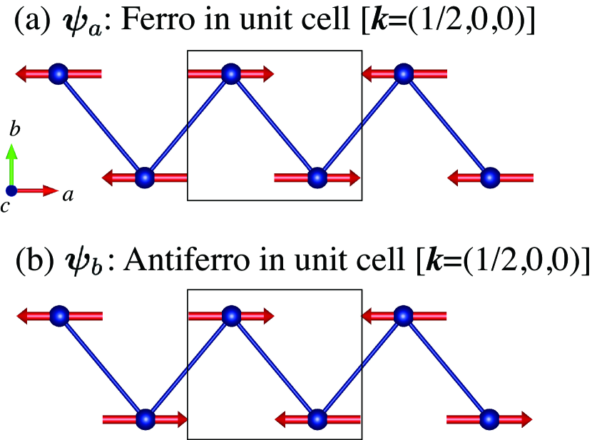
Figure 1: (a) Ferro and (b) antiferro magnetic structures in unit cell with $\bm{k}=(\frac{1}{2},0,0)$ on zigzag chain.

II.3 Magnetic structure generation for single-$\bm{k}$ states

Figure 2: Virtual clusters in space group $P4bm$.

Table 2: Atomic indices transformed by representative elements for space group $P4bm$.

	$\{E|\bm{0}\}$	$\{C_{2z}|\bm{0}\}$	$\{C_{4z}|\bm{0}\}$	$\{C^{-1}_{4z}|\bm{0}\}$
$i$	$1$	$1$	$1$	$1$
$\zeta$	$1$	$2$	$3$	$4$
$s_{i_{\zeta}}[1]$	$1$	$1$	$2$	$2$
$s_{i_{\zeta}}[2]$	$2$	$2$	$1$	$1$
	$\{IC_{2y}|\bm{\tau}\}$	$\{IC_{2x}|\bm{\tau}\}$	$\{IC_{2[1\bar{1}0]}|\bm{\tau}\}$	$\{IC_{2[110]}|\bm{\tau}\}$
$i$	$2$	$2$	$2$	$2$
$\zeta$	$1$	$2$	$3$	$4$
$s_{i_{\zeta}}[1]$	$2$	$2$	$1$	$1$
$s_{i_{\zeta}}[2]$	$1$	$1$	$2$	$2$

We first focus on single-$\bm{k}$ magnetic structure, whose periodicity is characterized by a single wave vector $\bm{k}$. At a given wave vector $\bm{k}$, the magnetic bases are classified into the IRREPs of the little group of $\bm{k}$ denoted as $\mathcal{G}_{\bm{k}}$. The group elements in $\mathcal{G}_{\bm{k}}$ are composed of a subset of symmetry operations in $\mathcal{G}$ which keeps $\bm{k}$ invariant under transformations. $\mathcal{G}_{\bm{k}}$ is thus a subgroup of a space group $\mathcal{G}$. We construct the $N_{\mathrm{coset}}$-virtual clusters, where each of them have $N_{h}$-atoms. By operating group elements $\left\{p_{i}|\bm{\tau}_{i}\right\}h_{\zeta}$ $(i=1,2,\ldots,N_{\mathrm{coset}},~{}\zeta=1,2,\ldots,N_{h})$ on a position vector $\bm{r}_{1}$, we can obtain $i$-th virtual cluster in which $\zeta$-th atom is indexed by $i_{\zeta}$ and the internal coordinates of $i_{\zeta}$-th atom is $\tilde{\bm{\eta}}_{{i}_{\zeta}}=p_{i}h_{\zeta}\bm{r}_{1}+\bm{\tau}_{i}$, where $\tilde{\bm{\eta}}_{i_{\zeta}}=\bm{r}_{1}$ for $i=1$ and $\zeta=1$ [22]. For clarity of this construction, virtual clusters in space group $P4bm$ are shown in Fig. 2 as an example. There are two sets of virtual clusters in this case, each of which consists of four atoms in square lattice arrangement since space group $P4bm$ is decomposed as $P4bm=\{E|\bm{0}\}\mathcal{H}\mathcal{T}+\{IC_{2y}|\bm{\tau}\}\mathcal{H}\mathcal{T}$ with $\mathcal{H}=(\{E|\bm{0}\},\{C_{2z}|\bm{0}\},\{C_{4z}|\bm{0}\},\{C^{-1}_{4z}|\bm{0}\})$ and $\bm{\tau}=(\frac{1}{2},\frac{1}{2},0)$.

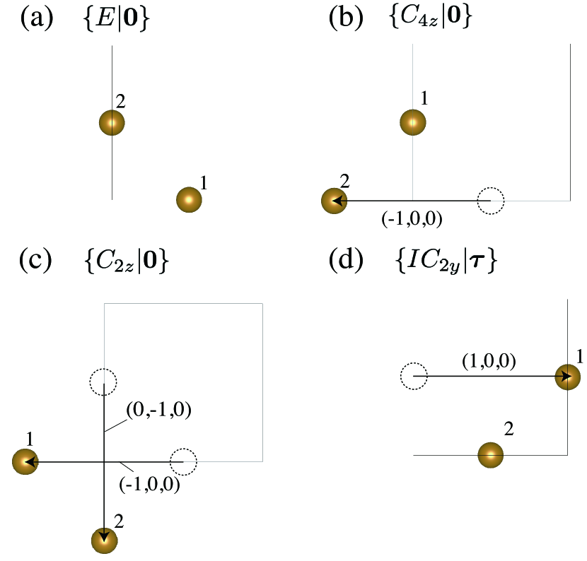
Figure 3: Transformation properties of atoms on $2b$-site in a crystallographic system with space group $P4bm$. The arrow represents primitive translation vector $\bm{R}^{\alpha}_{i_{\zeta}}$ associated with each space group operator (see main text).

To take account of the inter-unit cell spatial modulation characterized by a propagation vector $\bm{k}$, we consider the Fourier transform of magnetic bases as follows:

$$\bm{\psi}^{(X)}_{\bm{k}l\Gamma_{\mathrm{s}}\gamma_{\mathrm{s}}i}=\frac{1}{\sqrt{N}}\sum_{\bm{R}}\bm{\psi}^{(X)}_{\bm{R}l\Gamma_{\mathrm{s}}\gamma_{\mathrm{s}}i}e^{i\bm{k}\cdot\bm{R}},$$ (10)

$$\tilde{\bm{e}}^{\mathrm{axial}}_{\bm{k}i_{\zeta}}=\frac{1}{\sqrt{N}}\sum_{\bm{R}}\tilde{\bm{e}}^{\mathrm{axial}}_{\bm{R}i_{\zeta}}e^{i\bm{k}\cdot\bm{R}},$$ (11)

where $\tilde{\bm{e}}^{\mathrm{axial}}_{\bm{R}i_{\zeta}}$ is the axial unit vector located on the site $i_{\zeta}$ of virtual cluster with position $\tilde{\bm{\eta}}_{i_{\zeta}}+\bm{R}$, and $\bm{R}$ is the primitive translation vector assuming that the virtual clusters are periodically arranged. $\bm{\psi}_{\bm{R}l\Gamma_{\mathrm{s}}\gamma_{\mathrm{s}}i}$ are magnetic bases on the $i$-th virtual cluster whose centers are located on $\bm{R}+\bm{\tau}_{i}$ given as follows:

$$\bm{\psi}^{(X)}_{\bm{R}l\Gamma_{\mathrm{s}}\gamma_{\mathrm{s}}i} =\sum_{\zeta=1}^{N_{h}}\bm{u}^{(X)}_{l\Gamma_{\mathrm{s}}\gamma_{\mathrm{s}},i_{\zeta}}\cdot\tilde{\bm{e}}^{\mathrm{axial}}_{\bm{R}i_{\zeta}},$$ (12)

where $\Gamma_{\mathrm{s}}$ and $\gamma_{\mathrm{s}}$ represent IRREP of point group of a virtual cluster and its component, respectively.

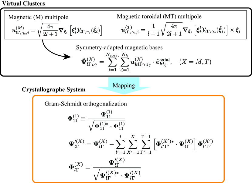
Figure 4: Outline of magnetic bases generation.

The coefficient $\bm{u}^{(X)}_{l\Gamma_{\mathrm{s}}\gamma_{\mathrm{s}},i_{\zeta}}$ is obtained by putting $p_{i}h_{\zeta}\bm{r}_{1}$ into $\bm{\xi}_{j}$ in Eqs. (6) and (7). We can construct the complex basis vectors having IRREPs under $\bm{k}$-group as linear combinations of the magnetic bases of Eq. (10) as follows:

$$\tilde{\bm{\Psi}}^{(X)}_{l\Gamma_{\bm{k}}\gamma} =\sum_{i=1}^{N_{\mathrm{coset}}}\sum_{\Gamma_{\mathrm{s}}\gamma_{\mathrm{s}}}C^{(X)}_{\bm{k}l\Gamma_{\mathrm{s}}\gamma_{\mathrm{s}}i;\Gamma\gamma}\bm{\psi}_{\bm{k}l\Gamma_{\mathrm{s}}\gamma_{\mathrm{s}}i}^{(X)}$$

$$=\sum_{i=1}^{N_{\mathrm{coset}}}\sum_{\zeta=1}^{N_{h}}\bm{u}^{(X)}_{l\Gamma_{\bm{k}}\gamma,i_{\zeta}}\cdot\tilde{\bm{e}}^{\mathrm{axial}}_{\bm{k}i_{\zeta}},$$ (13)

where $\Gamma_{\bm{k}}$ denotes the IRREPs of $\bm{k}$-group, $\gamma$ represents its component, $u^{(X)}_{l\Gamma_{\bm{k}}\gamma,\alpha\mu}$ is given as follows:

$$\bm{u}^{(X)}_{l\Gamma_{\bm{k}}\gamma,i_{\zeta}}=\sum_{\Gamma_{\mathrm{s}}\gamma_{\mathrm{s}}}C^{(X)}_{l\Gamma_{\mathrm{s}}\gamma_{\mathrm{s}}i;\Gamma_{\bm{k}}\gamma}\bm{u}^{(X)}_{l\Gamma_{\mathrm{s}}\gamma_{\mathrm{s}},i_{\zeta}}.$$ (14)

Note that coefficients $C_{l\Gamma_{\mathrm{s}}\gamma_{\mathrm{s}}i;\Gamma_{\bm{k}}\gamma}$ can be obtained using ordinary projection operator method to obtain the linear combination of atomic orbitals (LCAO) for the tight-binding model with wave vector $\bm{k}$ and IRREP $\Gamma_{\mathrm{s}}$ at site $i$ [23]. Complex magnetic basis $\bm{\Psi}^{(X)}_{l\Gamma_{\bm{k}}\gamma}$ in crystallographic systems can be obtained by mapping $\tilde{\bm{\Psi}}^{(X)}_{l\Gamma_{\bm{k}}\gamma}$ onto crystallographic lattices as follows:

$$\bm{\Psi}^{(X)}_{l\Gamma_{\bm{k}}\gamma} =\sum_{i=1}^{N_{\mathrm{coset}}}\sum_{\zeta=1}^{N_{h}}e^{-i\varphi^{\bm{k},1}_{i_{\zeta}}}\bm{u}^{(X)}_{l\Gamma_{\bm{k}}\gamma,i_{\zeta}}\cdot\bm{e}^{\mathrm{axial}}_{\bm{k}s_{i_{\zeta}}[1]},$$ (15)

where $\bm{e}^{\mathrm{axial}}_{\bm{k}\alpha}$ represents the Fourier component of axial unit vector on site $\alpha$ in the crystallographic system and $s_{i_{\zeta}}[\alpha]$ is the permutation operator for indices of atomic sites $\alpha$ associated with the symmetry operation $\{p_{i}h_{\zeta}|\bm{\tau}_{i}\}$, which transforms an atomic site of crystallographic system $\bm{\eta}_{\alpha}$ as follows: $\{p_{i}h_{\zeta}|\bm{\tau}_{i}\}\bm{\eta}_{\alpha}=\bm{\eta}_{s_{i_{\zeta}}[\alpha]}+\bm{R}^{\alpha}_{i_{\zeta}}$ with $\bm{R}^{\alpha}_{i_{\zeta}}$ being a primitive translation vector. $\alpha=1$ represents the atom mapped from an atom in virtual cluster with $i=1$ and $\zeta=1$. Transformation properties of atomic sites on $2b$-site in space group $P4bm$ are shown in Table 2 and Fig. 3 as an example. The phase factor $\varphi^{\bm{k},\alpha}_{i_{\zeta}}$ is given as $\varphi^{\bm{k},\alpha}_{i_{\zeta}}=\bm{k}\cdot\bm{R}^{\alpha}_{i_{\zeta}}$. We note that letting $N_{\mathrm{atom}}$ be the number of magnetic atoms in the crystallographic unit cell, each magnetic basis $\bm{\Psi}^{(X)}_{l\Gamma_{\bm{k}}\gamma}$ in Eq. (15) is $3N_{\mathrm{atom}}$-dimensional vector while $\tilde{\bm{\Psi}}^{(X)}_{l\Gamma_{\bm{k}}\gamma}$ in Eq. (13) is $3N_{0}$-dimensional one with $N_{0}\geq N_{\mathrm{atom}}$. The magnetic bases in Eq. (15) have transformation properties of IRREP $\Gamma_{\bm{k}}$ in $\bm{k}$-group $\mathcal{G}_{\bm{k}}$ as shown in Appendix A. We can obtain complete orthogonal symmetry-adapted magnetic structure basis set iteratively using Eqs. (6), (7), and (12)-(15) combined with the following Gram-Schmidt orthogonalization increasing rank $l$ from $l=1$ [2],

$$\bm{\Phi}^{(1)}_{11}\equiv\frac{\bm{\Psi}^{(1)}_{11}}{\sqrt{\bm{\Psi}^{({1})*}_{11}\cdot\bm{\Psi}^{(1)}_{11}}},$$ (16)

$$\bm{\Psi}^{\prime(X)}_{l\Gamma}=\bm{\Psi}^{(X)}_{l\Gamma}-\sum^{l}_{l^{\prime}=1}\sum^{X}_{X^{\prime}=1}\sum^{\Gamma-1}_{\Gamma^{\prime}=1}\left[\bm{\Phi}^{({X^{\prime}})*}_{l^{\prime}\Gamma^{\prime}}\cdot\bm{\Psi}^{(X)}_{l\Gamma}\right]\bm{\Phi}^{(X^{\prime})}_{l^{\prime}\Gamma^{\prime}},$$ (17)

$$\bm{\Phi}^{(X)}_{l\Gamma}=\frac{\bm{\Psi}^{\prime(X)}_{l\Gamma}}{\sqrt{\bm{\Psi}^{\prime({X})*}_{l\Gamma}\cdot\bm{\Psi}^{\prime(X)}_{l\Gamma}}},$$ (18)

where $\bm{\Phi}^{(X)}_{l\Gamma}$ is the orthonormal magnetic basis and we reexpress types of multipoles with $X=M$ and $T$ by the numbers $X=1$ and $2$, respectively, and abbreviately denote the IRREP of $\bm{k}$-group $\Gamma_{\bm{k}}$ and its component $\gamma$ by $\Gamma$. The magnetic bases generation procedure is summarized in Fig. 4. Although resultant magnetic bases are generally complex, we can always construct real (physical) magnetic bases by taking linear combinations of bases with $\bm{k}$ and $-\bm{k}$.

II.4 Multiple-$\bm{k}$ states

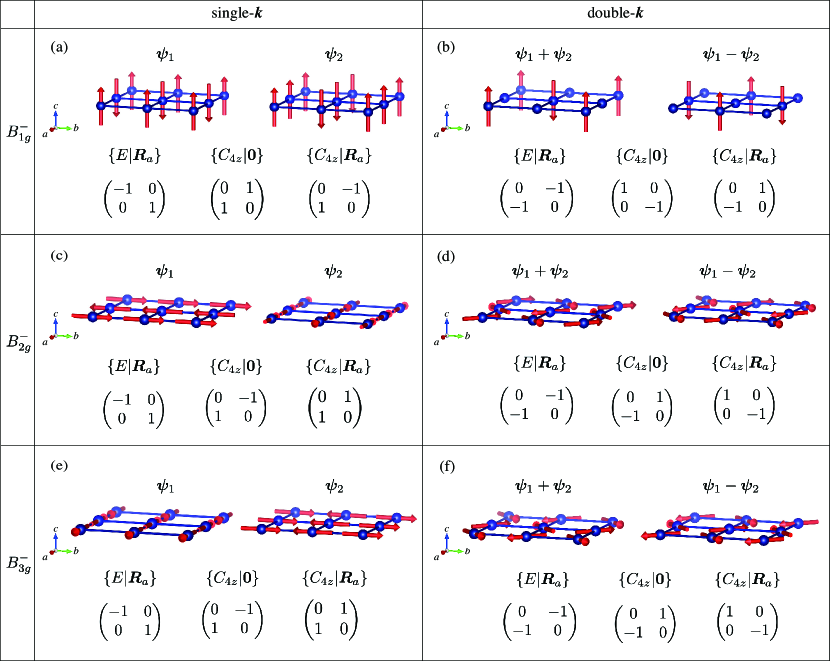
Figure 5: (a), (c), and (e) Single-$\bm{k}$ and (b), (d), and (f) double-$\bm{k}$ magnetic structures with $\bm{k}=(\frac{1}{2},0,0)$ and $(0,\frac{1}{2},0)$ on the square lattice. The representation matrices for symmetry operations $\{E|\bm{0}\}$, $\{C_{4z}|\bm{0}\}$, and $\{C_{4z}|\bm{R}_{a}\}$ with $\bm{R}_{a}=(1,0,0)$ are also shown.

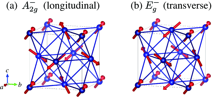
Figure 6: Triple-$\bm{k}$ magnetic structures on the FCC lattice induced from magnetic structures with $\bm{k}=(1,0,0)$ having (a) $A^{-}_{2g}$- and (b) $E^{-}_{g}$-representations.

A single-$\bm{k}$ magnetic structure with propagation vector $\bm{k}$ in an IRREP $\Gamma_{\bm{k}}$ of $\bm{k}$-group $\mathcal{G}_{\bm{k}}$ is a basis vector in an IRREP of $\mathcal{G}$, that is $(\Gamma_{\bm{k}}\!\uparrow\!\mathcal{G})\!\downarrow\!\mathcal{G}_{\bm{k}}=\Gamma_{\bm{k}}$ [11, 24]. Multiple-$\bm{k}$ magnetic structures are induced as bases of IRREPs in space group $\mathcal{G}$ from single-$\bm{k}$ magnetic structure bases with IRREPs in $\mathcal{G}_{\bm{k}}$ by taking account of the following relation between $\mathcal{G}_{\bm{k}}$ and $\mathcal{G}$ [11, 24]:

$$\mathcal{G}=\sum_{i=1}^{S_{\bm{k}}}\left\{p_{i}|\bm{\tau}_{i}\right\}\mathcal{G}_{\bm{k}},$$ (19)

where $\left\{p_{1}|\bm{\tau}_{1}\right\}=\left\{E|\bm{0}\right\}$ and $\left\{p_{i}|\bm{\tau}_{i}\right\}$ for $i\geq 2$ is the symmetry operation of space group $\mathcal{G}$ not included in $\bm{k}$-group $\mathcal{G}_{\bm{k}}$. The set of wave vectors $\bm{k}_{i}\equiv p_{i}\bm{k}$ $(i=1,2,\ldots,S_{\bm{k}})$ which are inequivalent with each other are called the star of $\bm{k}$. The bases in IRREP of $\mathcal{G}$ having propagation vector $\bm{k}_{i}$ can be generated by acting $\{p_{i}|\bm{\tau}_{i}\}$ on a single-$\bm{k}$ magnetic structure with IRREP $\Gamma_{\bm{k}}$ of $\mathcal{G}_{\bm{k}}$. Dimension of IRREPs of $\mathcal{G}$ is therefore equal to that of $\mathcal{G}_{\bm{k}}$ multiplied by $S_{\bm{k}}$. The multiple-$\bm{k}$ magnetic structures formed as linear combination of the symmetry-adapted single-$\bm{k}$ structures with propagation vectors associated with each other by symmetry operations $\left\{p_{i}|\bm{\tau}_{i}\right\}$ in Eq. (19) can preserve the higher rotational symmetry than that of the single-$\bm{k}$ structures, while it makes the translational symmetry lower than that under the single-$\bm{k}$ structures.

To gain a clear insight into multiple-$\bm{k}$ magnetic states, we here discuss two examples of multiple-$\bm{k}$ states: double-$\bm{k}$ states on the square lattice and triple-$\bm{k}$ states on the face centered cubic (FCC) structure. The double-$\bm{k}$ states having high magnetic point group symmetry with propagation vectors $\bm{k}=(\frac{1}{2},0,0)$ and $(0,\frac{1}{2},0)$ on the square lattice as well as the single-$\bm{k}$ states are shown in Fig. 5. The double $\bm{k}$-states are obtained as linear combinations of single-$\bm{k}$ states $\bm{\psi}_{1}$ and $\bm{\psi}_{2}$ as shown in Fig. 5. Note that the space group of the square lattice is $P4/mmm$ and point group preserving $\bm{k}$, referred as $\bm{k}$-point group, is $D_{2h}$. In this case, all IRREPs of $\mathcal{G}_{\bm{k}}$ are one-dimensional and $S_{\bm{k}}=2$, leading to two-dimensional IRREPs under $\mathcal{G}$. The representation matrices for several space group elements are also explicitly shown in Fig. 5. We can see that in the single-$\bm{k}$ (double-$\bm{k}$) states, the representation matrix for translational symmetry $\{E|\bm{R}_{a}\}$ with $\bm{R}_{a}=(1,0,0)$ has diagonal (non-diagonal) form, while that for rotational operation $\{C_{4z}|\bm{0}\}$ or $\{C_{4z}|\bm{R}_{a}\}$ has non-diagonal (diagonal) form. This indicates that the rotational symmetry in double-$\bm{k}$ states is higher than that in the single-$\bm{k}$ states but translational symmetry in the double-$\bm{k}$ states is lower than that in the single-$\bm{k}$ states, as mentioned before. It should be noted that time-reversal symmetry is retained macroscopically both in the single- and double-$\bm{k}$ states, that is, time-reversal operation combined with translational operation is preserved in the magnetic states. As a result, the magnetic point group in the double-$\bm{k}$ states shown in Fig. 5 is same as in the paramagnetic state, that is $4/mmm1^{\prime}$, whereas that in the single-$\bm{k}$ states is orthorhombic one $mmm1^{\prime}$, which is lower than $4/mmm1^{\prime}$. The breaking of four fold rotational symmetry along $z$-axis in the single-$\bm{k}$ states is understood from the uniaxial folding of the Brillouin zone along $x$- or $y$-direction from the paramagnetic state to magnetic state. This type of magnetic ordering causing breaking of four fold rotational symmetry has been discussed in the context of iron-pnictides [25, 26].

The examples of triple-$\bm{k}$ states with propagation vectors at the X-points, $\bm{k}_{1}=(1,0,0)$, $\bm{k}_{2}=(0,1,0)$, and $\bm{k}_{3}=(0,0,1)$, on FCC lattice are also shown in Figs. 6(a) and (b). The space group of FCC lattice is $Fm\bar{3}m$ and the $\bm{k}$-point group is $D_{4h}$. Note that the magnetic structure in Fig. 6(a) has been observed in Fe-Mn alloys [27, 28, 29] and several $f$-electron compounds such as Np$X$ ($X$=As, Sb, Bi) [30, 31, 32] and USb [33, 34]. In contrast to the square lattice discussed above, there are two types of two-dimensional IRREPs, $E^{-}_{g}$- and $E^{-}_{u}$-IRREPs, in addition to the eight types of one-dimensional IRREPs of $D_{4h}$ $\bm{k}$-point group at the X-points. Here and hereafter, we label the odd (even)-parity for time-reversal symmetry as superscript $-$ ($+$) in IRREPs such as $E^{-}_{g}$ ($E^{+}_{g}$). The two- and one-dimensional IRREPs under $\mathcal{G}_{\bm{k}}$ with $S_{\bm{k}}=3$ form six- and three-dimensional IRREPs under $\mathcal{G}$ since the X-points $(1,0,0)$, $(0,1,0)$, and $(0,0,1)$ are transformed into each other by symmetry operations $\{E|\bm{0}\}$, $\{C_{3[111]}|\bm{0}\}$, and $\{C^{2}_{3[111]}|\bm{0}\}$, where $C_{3[111]}$ is three fold rotation along $[111]$ direction. The single-$\bm{k}$ magnetic state with propagation vector $\bm{k}_{i}$ ($i=1,2,3$) preserves macroscopic time-reversal symmetry since $\bm{k}_{i}$ is a time-reversal invariant momentum. On the contrary, any linear combination of single-$\bm{k}$ magnetic bases with $\bm{k}_{i}$ to form triple-$\bm{k}$ states necessarily breaks macroscopic time-reversal symmetry. For instance, when a translational operation $\bm{t}$ carries the factor $-1$ for the magnetic bases with $\bm{k}_{1}$ and $\bm{k}_{2}$, and then same translation carries factor $+1$ for that with $\bm{k}_{3}=-\bm{k}_{1}-\bm{k}_{2}$. Since all the magnetic bases with $\bm{k}_{i}$ ($i=1,2,3$) cannot be simultaneously transformed into themselves with factor $-1$ under a primitive translation $\bm{t}$, the triple-$\bm{k}$ magnetic ordering breaks the macroscopic time-reversal symmetry. As a result, the triple-$\bm{k}$ magnetic order is accompanied with the secondary uniform magnetic order parameter, that is, magnetic multipoles with $\bm{k}=\bm{0}$. In the present case, triple-$\bm{k}$ magnetic ordering induces the secondary uniform magnetic order parameter having $A^{-}_{2g}$-IRREP of $O_{h}$ point group. The experimentally observed all-in-all-out type magnetic order in a pyrochlore oxide Cd₂Os₂O₇ with space group $Fd\bar{3}m$ [35] has the same symmetry of the secondary magnetic order parameter, $A^{-}_{2g}$, of the triple-$\bm{k}$ state in the FCC lattice, as shown in Fig. 6(a). Arima has pointed out that the all-in-all-out magnetic order can be regarded as a ferroic order of magnetic octupole $M_{xyz}$ and leads to several intriguing phenomena such as asymmetric magnetization and linear magnetostriction [36]. It is, therefore, expected that similar phenomena emerge also in Fe-Mn alloys, Np$X$, and USb. On the other hand, the triple-$\bm{k}$ state shown in Fig. 6(b) is induced from the magnetic structure with $E^{-}_{g}$-symmetry of $\bm{k}$-group at X-point. This type of magnetic ordering has been observed in UO₂ [37, 38]. This magnetic ordering with magnetic point group $m\bar{3}$ is absence of anti-unitary symmetry operations, which belongs to type-I Shubnikov group [11]. The absence of anti-unitary symmetry operations indicates that the axial (polar) tensors having opposite parities for time-reversal operation, that is, M- (MT-) and ET- (E-) multipoles cannot be distinguished from the symmetry viewpoint. These multipoles thus are simultaneously activated in this situation [39], resulting in intriguing physical phenomena. For instance, electric toroidal dipolar moment as well as the magnetic moment are linearly coupled with magnetic field in the magnetic state shown in Fig. 6(b). The crystal symmetry is thus lowered to $C_{2h}$ by magnetic field along $[001]$-axis in contrast to the case of similar paramagnetic point group $m\bar{3}1^{\prime}$, in which the crystal symmetry is lowered to $D_{2h}$ by magnetic field along $[001]$-axis. Such characteristic magnetostriction is useful for identifying the order parameter.

III Application to representative AHE antiferromagnets

III.1 $\alpha$-Mn

Figure 7: (a) Crystal structure and (b) first Brillouin zone of $\alpha$-Mn. Mn-I, -II, -III, and -IV sites are separately shown in panels (c), (d), (e), and (f), respectively, where body-centered sites are not shown.

Unary manganese forms various crystal structures depending on temperature, which are called $\alpha$-, $\beta$-, $\gamma$-, and $\delta$-Mn [40]. $\alpha$-Mn with body centered cubic (BCC) structure, which is realized at $T\lesssim$980\text{\,}\mathrm{K}$$, has attracted interest due to its intriguing and complex magnetic properties. A noncollinear antiferromagnetism with ordering vector $\bm{k}=\bm{k}_{\mathrm{H}}\equiv(1,0,0)$ is realized at $T\lesssim$95\text{\,}\mathrm{K}$$ [41, 42, 43, 44, 45] under an ambient pressure, while a first order transition to the another magnetic phase with tiny net magnetization $\sim 0.02~{}\mu_{\mathrm{B}}/\mathrm{Mn}$ takes place under an applied pressure $P\sim$1.4\text{\,}\mathrm{GPa}$$ [46, 47, 48]. The recent experimental study has revealed the emergence of large anomalous Hall response reaching $\sigma_{xy}\sim 400$-$600\text{\,}\mathrm{S}\text{\,}{\mathrm{cm}}^{-1}$ in the high pressure phase despite such small net magnetization [47]. We here apply our theory to $\alpha$-Mn to generate magnetic structures at high symmetry $\bm{k}$-points and provide a possible scenario for large anomalous Hall response in the high pressure magnetic phase, in which magnetic structure has not been clarified experimentally.

Table 3: Local magnetic moments in units of $\mu_{\mathrm{B}}$ on each Mn site in AFM phase in $\alpha$-Mn at ambient pressure from Ref. [45]. Note that Mn-III and Mn-IV sites are split into two different types of Mn sites due to lacking of $C_{3}$ symmetry in AFM phase.

	I	II	III-1	III-2	IV-1	IV-2
$m_{x}$	$0.0$	$0.14$	$0.43$	$-0.25$	$0.27$	$-0.08$
$m_{y}$	$0.0$	$0.14$	$0.43$	$-0.25$	$0.27$	$-0.45$
$m_{z}$	$2.83$	$1.82$	$0.43$	$-0.32$	$-0.45$	$-0.48$
$|\bm{m}|$	$2.83$	$1.83$	$0.74$	$0.48$	$0.59$	$0.66$

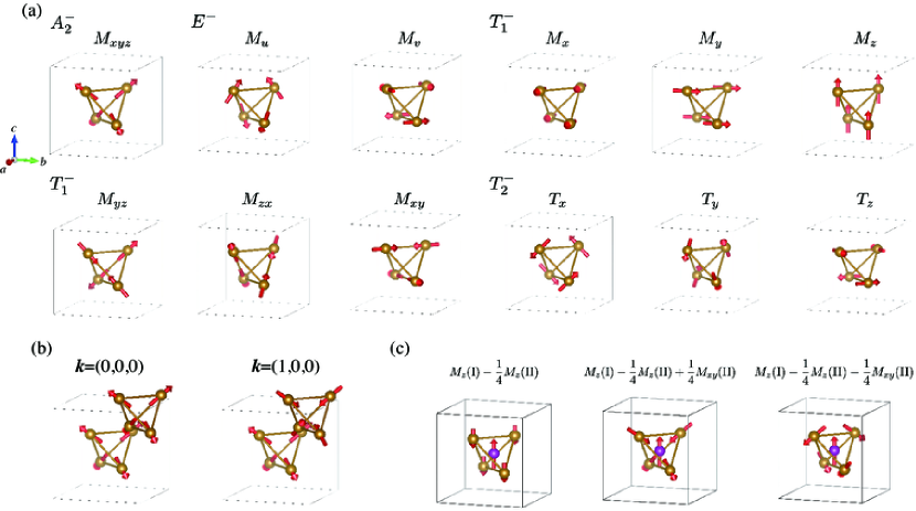
Figure 8: (a) Magnetic structure bases with $\bm{k}=\bm{0}$ on Mn-II sites in $\alpha$-Mn. (b) Comparison between magnetic basis having $A^{-}_{2}$-IRREP with $\bm{k}=\bm{0}$ and that with $\bm{k}=(1,0,0)$. (c) Examples of magnetic structures without net magnetization compatible with finite AHE $\sigma_{xy}\neq 0$.

Figure 7 shows crystal structure and the corresponding first Brillouin zone for $\alpha$-Mn. The primitive (conventional) unit cell contains 29 (58) Mn-atoms and resulting crystal structure is relatively complicated. The space group symmetry of $\alpha$-Mn is $I\bar{4}3m$ (No. 217, $T^{3}_{d}$), and there are four distinct types of Mn-sites, Mn-I, Mn-II, Mn-III, and Mn-IV sites which are located on $2a$, $8c$, $24g$, and $24g$ Wyckoff positions, respectively. The sizes of local magnetic moments largely depend on the types of Mn-sites according to experiments in the AFM phase at ambient pressure. The magnetic moments on Mn-I and -II sites are quite larger than those on Mn-III and -IV sites, as shown in Table 3 [43, 44, 45] and a similar tendency for local magnetic moments is obtained by the first-principles calculations [49, 50, 51, 52]. In addition, the internal magnetic fields on Mn-III and -IV sites are rapidly suppressed by an applied pressure according to the recent zero-field NMR measurements [53]. We thus focus on magnetic structures on Mn-I and -II sites in this paper.

Nonzero anomalous Hall response requires symmetry breaking same as ferromagnetic ordering, which belongs to $T^{-}_{1}$-IRREP with $\bm{k}=\bm{0}$ under $T_{d}$-point group in the present system [1, 54, 55, 56, 21, 39]. According to the recent neutron diffraction measurements, the magnetic reflection observed in the ambient pressure phase is absent in the high pressure phase [57]. Therefore, we focus on the cases of magnetic orderings having $T^{-}_{1}$ symmetry with ordering vector $\bm{k}=\bm{0}$ and $\bm{k}=\bm{k}_{\mathrm{H}}=(1,0,0)$ in the present study.

The transformation properties for arbitrary magnetic structures on each Wyckoff position are encoded in representation matrices, which are called magnetic representations. The magnetic representations of $2a$ and $8c$-sites, $D^{(\mathrm{mag})}_{2a}$ and $D^{(\mathrm{mag})}_{8c}$, are decomposed into IRREPs of $\mathcal{G}_{\bm{k}}$ with $\bm{k}=\bm{0}$ as follows:

$$D^{(\mathrm{mag})}_{2a}=T^{-}_{1},$$ (20)

$$D^{(\mathrm{mag})}_{8c}=A^{-}_{2}\oplus E^{-}\oplus 2T^{-}_{1}\oplus T^{-}_{2},$$ (21)

where we use Mulliken notation for IRREPs under $T_{d}$ point group since IRREPs of $\mathcal{G}_{\bm{k}}$ with $\bm{k}=\bm{0}$ are equivalent to those of crystallographic point group of $\mathcal{G}$. We show the symmetry-adapted magnetic structures at $8c$-site with $\bm{k}=\bm{0}$ in Fig. 8(a). Note that the magnetic structures having $\bm{k}=\bm{k}_{\mathrm{H}}$ can be obtained by reversing magnetic moments on body center tetrahedra for those with $\bm{k}=\bm{0}$ as shown in Fig. 8(b). The obtained magnetic structure bases with $\bm{k}=\bm{k}_{\mathrm{H}}$ are consistent with the preceding group theoretical analysis of neutron diffraction experiment [42].

From Eqs. (20) and (21) and Fig. 8(a), we can see that there are two sets of magnetic structure bases on $8c$-site with $T^{-}_{1}$-IRREP whereas there is one set of magnetic structures on $2a$-site with $T^{-}_{1}$-IRREP, that is, ferromagnetic structure. One of $T^{-}_{1}$-IRREP magnetic structures on $8c$-site corresponds to the ordinary ferromagnetism, and the other is noncollinear AFM without net magnetization. The linear combinations of these magnetic bases can generate nonzero anomalous Hall response $\sigma_{xy}\neq 0$. The magnetic structures without net magnetization are shown in Fig. 8(c).

Table 4: Band deformation and macroscopic responses in the magnetic ordered phases having $T^{-}_{1}$-IRREP with the ordering vectors $\bm{k}=\bm{0}$ ($\Gamma$-point) in the high pressure phase and $\bm{k}=\bm{k}_{\mathrm{H}}$ ($\mathrm{H}$-point) in the ambient pressure phase. AHE, ANE, ME, MC, and MOKE represent anomalous Hall, anomalous Nernst, magneto-electric, magneto-current, and magneto-optical Kerr effects, respectively. Note that magneto-current effects correspond to Edelstein effect and its inverse response.

ordering vector	band deformation				macroscopic response
$\Gamma:(0,0,0)$	$(3k^{2}_{z}-k^{2})\sigma_{0}$	$k_{x}\sigma_{x}-k_{y}\sigma_{y}$	$\sigma_{z}$	$k_{z}(k_{x}^{2}-k_{y}^{2})\sigma_{0}$	AHE, ANE, MOKE, ME, MC
$\mathrm{H}:(1,0,0)$	$(3k^{2}_{z}-k^{2})\sigma_{0}$	$k_{x}\sigma_{x}-k_{y}\sigma_{y}$	✗	✗	MC

We here discuss the secondary order parameters based on the Landau theory [58, 59], which gives clear insight into physical phenomena in the ordered phases and useful information about primary order parameters. In fact, detailed analysis for couplings between primary and secondary order parameters leads to deep understanding of complex multipolar ordered phases in the $f$-electron systems [20, 60, 61, 62, 63]. The possible secondary order parameters are characterized by $\bm{k}=\bm{0}$ in case the primary order parameter has the ordering vector $\bm{k}=\bm{0}$. We first discuss the electric degrees of freedom induced by the magnetic orderings, which are relevant to elastic response and Edelstein effect, for instance. The electric order parameters, which are time-reversal-even, are induced by the coupling of the electric multipoles to the even order terms of magnetic ones in Landau free energy expression due to the time-reversal symmetry in the paramagnetic phase. The electric order parameters emerging through the lowest third order terms, can be deduced by irreducible decomposition of symmetric product of primary order parameters as follows:

$$[T^{-}_{1}\otimes T^{-}_{1}]=A^{+}_{1}\oplus E^{+}\oplus T^{+}_{2},$$ (22)

where the secondary order parameters with $A^{+}_{1}$, $E^{+}$, and $T^{+}_{2}$-IRREPs correspond to uniform electric monopole $Q_{0}$, electric quadrupoles $(Q_{u(=3z^{2}-r^{2})},Q_{v(=x^{2}-y^{2})})$, and $(Q_{yz},Q_{zx},Q_{xy})$, respectively from the symmetry viewpoint. Note that in the present case, electric toroidal quadrupole (electric dipole) $(G_{v},G_{u})$ [$(Q_{x},Q_{y},Q_{z})$] also emerges when electric quadrupole $(Q_{u},Q_{v})$ [$(Q_{yz},Q_{zx},Q_{xy}$)] is finite since those have the same IRREP $E^{+}$ ($T^{+}_{2}$) under $T_{d}$ point group. The explicit forms of the third order terms in Landau free energy are given as follows:

$$F^{(3)} =c_{1}\left[M_{y}M_{z}Q_{yz}+(\mathrm{cyclic~{}perm.})\right]$$

$$+c_{2}\sqrt{3}\left(M^{2}_{x}-M^{2}_{y}\right)Q_{v}$$

$$+c_{2}\left(2M^{2}_{z}-M^{2}_{x}-M^{2}_{y}\right)Q_{u},$$ (23)

where we neglect trivial coupling with the fully symmetric $Q_{0}$ term and $(\mathrm{cyclic~{}perm.})$ represents the terms obtained by cyclic permutations for indices of $M_{y}M_{z}Q_{yz}$ as $x,y,z\to y,z,x$ and $z,x,y$, and $c_{1}$ and $c_{2}$ are coupling constants determined from microscopic models. Eq. (23) represents that the electric quadrupole is inevitably induced by primary order parameter with $T^{-}_{1}$-IRREP. For example, $Q_{u}$-type electric quadrupole emerges in the case that $M_{x}=M_{y}=0$ and $M_{z}\neq 0$ while the electric quadrupoles having $T^{+}_{2}$ symmetry emerge with the same amplitude of all components, that is, $Q_{yz}=Q_{zx}=Q_{xy}\neq 0$ in the case that $M_{x}=M_{y}=M_{z}\neq 0$. Therefore, the symmetry of crystal structure is lowered to tetragonal $D_{2d}$ point group in the former case, which can induce gyrotropic magnetic effect, and polar trigonal $C_{3v}$ point group in the latter case. Note that similar couplings to electric multipoles with $\bm{k}=\bm{0}$ emerges also in the case of the primary order parameter with $\bm{k}=\bm{k}_{\mathrm{H}}$ since the even powers of primary order parameters carry the wave vector $\bm{k}=\bm{0}$ modulo reciprocal lattice vector.

In the similar manner, secondary magnetic order parameters are discussed. Due to the time reversal symmetry in the nonmagnetic phase, the secondary magnetic order parameter emerges through the fourth order coupling in the Landau free energy, which can be obtained by the irreducible decomposition of fully symmetric product $[T^{-}_{1}\otimes T^{-}_{1}\otimes T^{-}_{1}]$ as follows:

$$[T^{-}_{1}\otimes T^{-}_{1}\otimes T^{-}_{1}]=A^{-}_{2}\oplus 2T^{-}_{1}\oplus T^{-}_{2},$$ (24)

where $A^{-}_{2}$ and $T^{-}_{2}$ correspond to magnetic octupoles $M_{xyz}$ and $(M^{\beta}_{x},M^{\beta}_{y},M^{\beta}_{z})$ from the symmetry viewpoint. The fourth order term of Landau free energy which represent coupling of order parameter with $T^{-}_{1}$-IRREP to the secondary order parameters having different symmetry is given as follows:

$$F^{(4)} =d_{1}M_{x}M_{y}M_{z}M_{xyz}$$

$$+d_{2}\left[\left(M^{2}_{y}-M^{2}_{z}\right)M_{x}M^{\beta}_{x}+(\mathrm{cyclic~{}perm.})\right].$$ (25)

From the above equation, we can see that in the case of $M_{x}=M_{y}=0$ and $M_{z}\neq 0$, the magnetic secondary order parameter does not emerge while in the case of $M_{x}=M_{y}=M_{z}\neq 0$ ($M_{z}=0$ and $M_{x}=M_{y}\neq 0$), the magnetic octupole $M_{xyz}$ ($M^{\beta}_{x}=-M^{\beta}_{y}$) is induced. On the other hand, when the primary order parameter has a modulation vector $\bm{k}=\bm{k}_{\mathrm{H}}$, secondary magnetic order parameters with $\bm{k}=\bm{0}$ do not emerge since combined symmetry of time-reversal operation and primitive translation retains in the ordered phase. The secondary induced magnetic multipoles have ordering vector $\bm{k}=\bm{k}_{\mathrm{H}}$ in this case.

The primary order parameters with inducing the secondary order parameters discussed above give rise to deformation of electronic states and resulting physical phenomena in the ordered phases. In particular, the order parameters with the ordering vector $\bm{k}=\bm{0}$ are important since those can be sources of macroscopic responses according to Neumann’s principle [64, 54, 56, 21] and experiments using macroscopic probes can detect the order parameters relatively easier. The magnetic order parameter $M_{z}$ with $\bm{k}=\bm{0}$ is finite in the high pressure phase, while that vanishes in the ambient pressure phase. The former case leads to anomalous Hall, Nernst effects, and magneto-optical effects. On the other hand, electric order parameters $Q_{u}$ and $G_{v}$ with $\bm{k}=\bm{0}$ can be finite in both ambient and high pressure magnetic phases. This gives rise to the antisymmetric spin-splitting of band structures $k_{x}\sigma_{x}-k_{y}\sigma_{y}$, resulting in natural optical activity and magneto-current effect such as Edelstein effect [65, 66, 67], where $\sigma_{i}$ ($i=x,y,z$) is the Pauli spin matrix. We summarize band deformations as the hopping terms in the $2\times 2$ Hamiltonian with spin degree of freedom and macroscopic responses in the ordered phases in Table 4.

III.2 Co$M_{3}$S₆

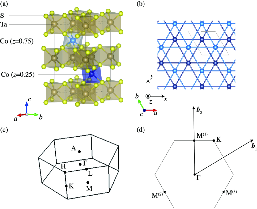
Figure 9: (a) Crystal structure of CoTa₃S₆ and (b) that on $ab$-plane with only Co-atoms. (c) First Brillouin zone for CoTa₃S₆ and (d) that on $k_{z}=0$ plane, where several high symmetry $\bm{k}$-points are shown by dots.

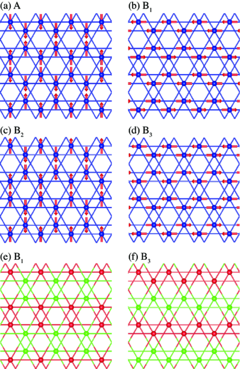
Figure 10: Magnetic structure bases with single-$\bm{k}$ $(0,\frac{1}{2},0)$ in crystal structure of Co$M_{3}$S₆. The arrow and red (green) sphere represents magnetic moment in $ab$-plane and along $+z$ ($-z$) axis, respectively.

.

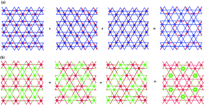
Figure 11: Triple-$\bm{k}$ magnetic structures induced from single-$\bm{k}$ magnetic bases with $B_{1}^{-}$ symmetry at M-points. Panels (a) and (b) correspond to those from magnetic bases shown in Figs. 10(b) and (e), respectively.

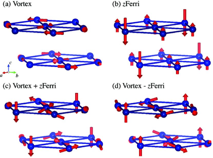
Figure 12: Examples of linear combinations of triple-$\bm{k}$ states shown in Fig. 11.

An intercalated compound of transition metal dichalcogenides, $TM_{3}$S₆ ($T$ = $3d$-transition metal, $M$ = Nb, Ta), shows rich electronic and magnetic properties. For instance, a helimagnetic ordering with a long period is formed in Cr$M_{3}$S₆ [68], which is transformed into chiral soliton lattice under a magnetic field. Another compound, ferromagnetic VNb₃S₆ is proposed as a candidate of Weyl semimetals by first-principles calculations [69]. CoNb₃S₆ in particular has attracted growing interests due to its large anomalous Hall conductivity in the magnetic ordered phase with a tiny ferromagnetic moment [70, 71, 72]. This compound crystallizes in the space group $P6_{3}22$ (No. 182, $D^{6}_{6}$) symmetry, where the crystal structure is shown in Fig. 9. Early neutron diffraction studies by Parkin et al. indicate the magnetic structure with a single-$\bm{k}$ $\left(0,\frac{1}{2},0\right)$ having multidomain for CoNb₃S₆ and that with $\bm{k}=\left(\frac{1}{3},\frac{1}{3},0\right)$ for CoTa₃S₆ [73]. Recent neutron diffraction patterns for CoNb₃S₆, however, are also compatible with multi-$\bm{k}$ magnetic order with single domain [71]. We here discuss possible magnetic structures with ordering vector $\bm{k}$ at high symmetry points in BZ and provide a symmetry analysis of magnetic structures in connection with emergence of anomalous Hall effect.

Let us consider magnetic structures with ordering vectors $\bm{k}$ at M-points. There are three symmetry equivalent M-points in the first Brillouin zone, which are given by $\bm{k}_{\mathrm{M}^{(1)}}=\left(0,\frac{1}{2},0\right)$, $\bm{k}_{\mathrm{M}^{(2)}}=\left(-\frac{1}{2},0,0\right)$, and $\bm{k}_{\mathrm{M}^{(3)}}=\left(\frac{1}{2},-\frac{1}{2},0\right)$ as shown in Figs. 9(c) and (d). The $\bm{k}$-point group at M-points is $D_{2}$ and magnetic bases can be classified according to IRREPs under this point group (see Table 5). Figure 10 shows symmetry adapted magnetic structures with a single propagation vector $\bm{k}=\bm{k}_{\mathrm{M}^{(1)}}$. All the magnetic structures in Fig. 10 are collinear AFM. Note that we can construct noncollinear magnetic structures as linear combinations of (b) and (e) and those of (d) and (f) without further symmetry lowering since the magnetic structures in Figs. 10(b) and (e) and those in (d) and (f) have same IRREPs. Symmetry operation of time-reversal combined with primitive lattice translation holds in the magnetic states characterized by $\bm{k}=(0,\frac{1}{2},0)$ shown in Fig. 10. As a result, anomalous Hall response is prohibited in these magnetic states.

Table 5: Character table for $\bm{k}$-group at $\mathrm{M}^{(i)}$-point. $C_{2x,1}$ and $C_{2y,1}$ represent two-fold rotation along $x$- and $y$-axes. $C_{2x(y),i}$ ($i=2,3$) is defined as $C_{2x(y),i}=C^{i-1}_{3z}C_{2x(y),1}C^{-i+1}_{3z}$.

	$E$	$C_{2z}$	$C_{2y,i}$	$C_{2x,i}$
$A$	$1$	$1$	$1$	$1$
$B_{1}$	$1$	$1$	$-1$	$-1$
$B_{2}$	$1$	$-1$	$1$	$-1$
$B_{3}$	$1$	$-1$	$-1$	$1$

As mentioned in Sec. II-C, triple-$\bm{k}$ magnetic structures are obtained from single-$\bm{k}$ magnetic bases. Possible high-symmetry triple-$\bm{k}$ magnetic structures related to anomalous Hall effect are shown in Fig. 11. The two magnetic structures, i.e., vortex-like arrangement of magnetic moments in $ab$-plane and ferrimagnetic structure along $c$-axis shown in Fig. 11, can induce AHE since these magnetic point groups are $62^{\prime}2^{\prime}$ [74]. The other high-symmetry triple-$\bm{k}$ magnetic states induced from single-$\bm{k}$ magnetic states having each of $A^{-}$, $B^{-}_{2}$, and $B^{-}_{3}$ symmetry in Table 5 prohibit AHE since these magnetic point groups are $622$, $6^{\prime}2^{\prime}2$, and $6^{\prime}22^{\prime}$, respectively [74]. The Landau free energy expression gives more clear insight into emergence of AHE in magnetically ordered phase. Secondary magnetic order parameters are coupled with the primary ones through the even order terms in the Landau free energy due to time-reversal symmetry in the paramagnetic state. Magnetic multipoles with $\bm{k}=\bm{0}$ are coupled with magnetic order parameters with $\bm{k}_{\mathrm{M^{(i)}}}$ through the fourth order terms in the Landau free energy since the sum of the wave vectors at M-points is zero: $\bm{k}_{\mathrm{M}^{(1)}}+\bm{k}_{\mathrm{M}^{(2)}}+\bm{k}_{\mathrm{M}^{(3)}}=\bm{0}$. In the case that primary order parameters have $B^{-}_{1}$ symmetry with propagation vector at M-points, the fourth order term in the Landau free energy is given as follows:

$$F^{(4)} =d_{1}M_{B^{(1)}_{1}}M_{B^{(2)}_{1}}M_{B^{(3)}_{1}}M_{z}$$

$$+d_{2}\left(M^{2}_{B^{(2)}_{1}}-M^{2}_{B^{(3)}_{1}}\right)M_{B^{(1)}_{1}}M_{A^{(1)}}$$

$$+d_{2}\left(M^{2}_{B^{(3)}_{1}}-M^{2}_{B^{(1)}_{1}}\right)M_{B^{(2)}_{1}}M_{A^{(2)}}$$

$$+d_{2}\left(M^{2}_{B^{(1)}_{1}}-M^{2}_{B^{(2)}_{1}}\right)M_{B^{(3)}_{1}}M_{A^{(3)}},$$ (26)

where $M_{A^{(i)}}$ and $M_{B^{(i)}_{1}}$ represent the magnetic order parameters having $A^{-}$- and $B^{-}_{1}$-symmetry with ordering vector $\bm{k}=\bm{k}_{\mathrm{M}^{(i)}}$, respectively, and $M_{z}$ represents the magnetic order parameter having $A^{-}_{2}$-symmetry with ordering vector $\bm{k}=\bm{0}$, i.e., the order parameter with same symmetry for $z$-component of net magnetization. The Eq. (26) clearly shows that uniform $M_{z}$ can be finite in the triple-$\bm{k}$ magnetic states induced from single-$\bm{k}$ magnetic states having $B^{-}_{1}$-symmetry, indicating the emergence of AHE $\sigma_{xy}\neq 0$ in the ordered phase though $M_{z}$ is not necessary to be finite. Note that magnetic toroidal dipole $T_{z}$ can be finite with $M_{z}$ since $T_{z}$ belongs to the same $A_{2}^{-}$-IRREP of $M_{z}$ in the present crystal structure having chiral point group $D_{6}$. The vortex-like arrangements of magnetic moments can be regarded as toroidal dipole moments [75, 76], and this is consistent with the magnetic structure shown in Fig. 11(a). The existence of magnetic toroidal dipole moments allows the magneto-electric effect and non-reciprocal charge transport, and these macroscopic responses can be footprints of triple-$\bm{k}$ ordering in the present case.

As mentioned in the previous subsection, the electric order parameters are coupled with magnetic ones through the odd order terms in Landau free energy. The third order terms are given as follows:

$$F^{(3)} =c_{1}\left(2M^{2}_{B^{(1)}_{1}}-M^{2}_{B^{(2)}_{1}}-M^{2}_{B^{(3)}_{1}}\right)Q_{v}$$

$$+c_{1}\sqrt{3}\left(-M^{2}_{B^{(2)}_{1}}+M^{2}_{B^{(3)}_{1}}\right)Q_{xy}$$

$$+c_{2}M_{B^{(2)}_{1}}M_{B^{(3)}_{1}}Q_{A^{(1)}}$$

$$+c_{2}M_{B^{(3)}_{1}}M_{B^{(1)}_{1}}Q_{A^{(2)}}$$

$$+c_{2}M_{B^{(1)}_{1}}M_{B^{(2)}_{1}}Q_{A^{(3)}},$$ (27)

where $(Q_{xy},Q_{v})$ is the electric multipole having $E^{+}_{2}$-symmetry with propagation vector $\bm{k}=\bm{0}$ and $Q_{A^{(i)}}$ represents electric order parameter having $A^{+}$-symmetry with $\bm{k}=\bm{k}_{\mathrm{M}^{(i)}}$. We can see that, from Eq. (27), single-$\bm{k}$ magnetic state $M_{B^{(1)}_{1}}\neq 0$ and $M_{B^{(2)}_{1}}=M_{B^{(3)}_{1}}=0$ break the crystallographic point group from hexagonal group $D_{6}$ to orthorhombic one $D_{2}$ and leads to the emergence of the secondary electric order parameter $Q_{v}$. The triple-$\bm{k}$ state, $M_{B^{(2)}_{1}}=M_{B^{(2)}_{1}}=M_{B^{(3)}_{1}}\neq 0$, preserves the crystallographic point group $D_{6}$, and the electric multipoles with $\bm{k}=\bm{0}$ are not induced as a result. Note that the unit cell in the triple-$\bm{k}$ state is extended in the $ab$-plane from the nonmagnetic one though the triple-$\bm{k}$ state has the same crystallographic point group with that for the nonmagnetic state. The resulting finite components of macroscopic response tensors associated with electric order parameters are thus unchanged from those in the paramagnetic phase. Meanwhile, the electric order parameters with $\bm{k}=\bm{k}_{\mathrm{M}^{(i)}}$ emerges $Q_{A^{(1)}}=Q_{A^{(2)}}=Q_{A^{(3)}}\neq 0$. These order parameters $Q_{A^{(i)}}$ corresponds to charge ordering with the propagation vector $\bm{k}_{\mathrm{M}^{(i)}}$ and can be measured by the microscopic probes such as X-ray diffraction measurements. Thus, the secondary order parameters are useful for gaining information about primary order ones also in this case.

IV Summary and outlook

We have proposed a generation method of symmetry-adapted magnetic structure basis set with finite propagation vector $\bm{k}$ based on multipole expansion. In this method, the magnetic configurations on a virtual cluster of each propagation vector is first generated with use of multipole expansion and then these are mapped onto crystallographic systems with a phase factor to take into consideration of spatial modulation of magnetic structures specified by a wave vector $\bm{k}$. The iterative implementation of this procedure with Gram-Schmidt orthogonalization provides complete orthonormal magnetic bases with a given $\bm{k}$ classified according to irreducible representations under $\bm{k}$-group in arbitrary crystal structures. We can also construct the multi-$\bm{k}$ magnetic structures as the induced representation of the single-$\bm{k}$ states. The obtained magnetic structures can be good candidates for initial magnetic configurations for density functional theory (DFT) calculations [12] and thus high-throughput DFT calculations for magnetic materials combined with the present magnetic basis generation method is a possible future direction of our work.

The present method is applied to representative materials $\alpha$-Mn and Co$M_{3}$S₆ ($M$ = Nb, Ta) showing large anomalous Hall effect (AHE) with tiny net magnetization. It is demonstrated that magnetic structures compatible with both AHE and small ferromagnetic moment can be constructed. We also discuss the secondary order parameter, physical responses, and electronic properties under magnetic orders in $\alpha$-Mn and Co$M_{3}$S₆. We show that various phenomena such as AHE, anomalous Nernst effect (ANE), and magneto-optical Kerr effect (MOKE) can emerge through the primary magnetic order parameter having $T_{1}^{-}$-symmetry with $\bm{k}=\bm{0}$ for high-pressure phase in $\alpha$-Mn, and the Edelstein effect driven by the odd parity electric order parameters are possible both in the ambient and high pressure phases since the symmetry of secondary electric order parameters are same in both phases. For Co$M_{3}$S₆, the magnetic order parameter with $T_{1}^{-}$-symmetry with $\bm{k}=\bm{0}$ are induced as a secondary order parameter in triple-$\bm{k}$ state, leading to emergence of AHE, ANE, MOKE, and non-reciprocal charge transport.

Our method is applicable to general magnets including noncollinear and noncoplanar antiferromagnets and skyrmion crystals [13]. The present magnetic structure generation scheme thus would facilitate exploration of functional magnetic materials.

Appendix A Transformation properties of $\bm{\Psi}_{l\Gamma_{\bm{k}}\gamma}$

In this appendix, we show that $\bm{\Psi}^{(X)}_{l\Gamma_{\bm{k}}\gamma}$ in Eq. (15) belongs to $\Gamma_{\bm{k}}$-IRREP. Since magnetic bases on virtual cluster $\tilde{\Psi}_{l\Gamma_{\bm{k}}\gamma}$ have transformation properties of IRREP $\Gamma_{\bm{k}}$, we should show the following relation: $\{p_{i}h_{\zeta}|\bm{\tau}_{i}\}\bm{\Psi}^{(X)}_{l\Gamma_{\bm{k}}\gamma}=\sum_{\gamma^{\prime}}D^{\Gamma_{\bm{k}}}_{\gamma^{\prime}\gamma}(\{p_{i}h_{\zeta}|\bm{\tau}_{i}\})\bm{\Psi}^{(X)}_{l\Gamma_{\bm{k}}\gamma^{\prime}}$, where $\{p_{i}h_{\zeta}|\bm{\tau}_{i}\}\in\mathcal{G}_{\bm{k}}$. The basis $\bm{e}^{\mathrm{axial}}_{\bm{k}\alpha\mu}$ have the following transformation properties under a $\bm{k}$-group operation $\{p_{i}h_{\zeta}|\bm{\tau}_{i}\}$,

$$\{p_{i}h_{\zeta}|\bm{\tau}_{i}\}\bm{e}^{\mathrm{axial}}_{\bm{k}\alpha\mu}=\sum_{\nu}D^{(\mathrm{axial})}_{\nu\mu}(p_{i}h_{\zeta})e^{-i\varphi^{\bm{k},\alpha}_{i_{\zeta}}}\bm{e}^{\mathrm{axial}}_{\bm{k}s_{i_{\zeta}}[\alpha]\nu},$$ (28)

where $D^{(\mathrm{axial})}$ is the transformation matrix of axial vector. We here note that the following relation for $\bm{R}^{s_{I^{\prime}}[\alpha]}_{I_{\bm{k}}}$ is satisfied,

$$\bm{R}^{s_{i_{\zeta}^{\prime}}[\alpha]}_{i_{\zeta}} =\{p_{i}h_{\zeta}|\bm{\tau}_{i}\}\bm{\eta}_{s_{i_{\zeta}^{\prime}}[\alpha]}-\bm{\eta}_{s_{i_{\zeta}}[s_{i_{\zeta}^{\prime}}[\alpha]]}$$

$$=\{p_{i}h_{\zeta}|\bm{\tau}_{i}\}\{p_{i^{\prime}}h_{\zeta^{\prime}}|\bm{\tau}_{i^{\prime}}\}\bm{\eta}_{\alpha}-p_{i}h_{\zeta}\bm{R}^{\alpha}_{i_{\zeta}^{\prime}}-\bm{\eta}_{s_{i_{\zeta}^{\prime\prime}}[\alpha]}$$

$$=\{p_{i^{\prime\prime}}h_{\zeta^{\prime\prime}}|\bm{\tau}_{i^{\prime\prime}}\}\bm{\eta}_{\alpha}+\bm{T}-p_{i}h_{\zeta}\bm{R}^{\alpha}_{i_{\zeta}^{\prime}}-\bm{\eta}_{s_{i_{\zeta}^{\prime\prime}}[\alpha]},$$ (29)

where symmetry operation $p_{i^{\prime\prime}}h_{\zeta^{\prime\prime}}$ and a primitive translation $\bm{T}$ are given as follows:

$$p_{i^{\prime\prime}}h_{\zeta^{\prime\prime}}=p_{i}h_{\zeta}p_{i^{\prime}}h_{\zeta^{\prime}},$$ (30)

$$\bm{T}=p_{i}h_{\zeta}\bm{\tau}_{i^{\prime}}+\bm{\tau}_{i}-\bm{\tau}_{i^{\prime\prime}}.$$ (31)

By taking account of the relations in Eqs. (29), (30), and (31), it is shown that $\left\{p_{i}h_{\zeta}|\bm{\tau}_{i}\right\}\bm{\Psi}^{(X)}_{l\Gamma_{\bm{k}}\gamma}$ is written as follows:

$$\{p_{i}h_{\zeta}|\bm{\tau}_{i}\}\bm{\Psi}^{(X)}_{l\Gamma_{\bm{k}}\gamma}$$

$$=\sum_{i^{\prime}=1}^{N_{\mathrm{coset}}}\sum_{\zeta^{\prime}=1}^{N_{h}}\sum_{\mu,\nu}e^{-i\varphi^{\bm{k},1}_{i_{\zeta}^{\prime\prime}}-i\bm{k}\cdot\bm{T}}$$

$$\times D^{(\mathrm{axial})}_{\mu\nu}(p_{i}h_{\zeta})u^{(X)}_{\bm{k}l\Gamma\gamma,i_{\zeta}^{\prime}\nu}\bm{e}^{\mathrm{axial}}_{\bm{k}s_{i_{\zeta}^{\prime\prime}}[1]\mu}.$$ (32)

Let us here derive the relation among $D^{\Gamma_{\bm{k}}}_{\gamma\gamma^{\prime}}$, $D^{(\mathrm{axial})}_{\mu\nu}$, and $u^{(X)}_{\bm{k}l\Gamma\gamma,\alpha\nu}$ from the transformation properties of magnetic bases on virtual cluster $\tilde{\bm{\Psi}}^{(X)}_{l\Gamma_{\bm{k}}\gamma}$. Similarly to Eq. (28), the magnetic bases $\tilde{\bm{e}}^{\mathrm{axial}}_{\bm{k}i_{\zeta}^{\prime}\mu}$ are transformed under a symmetry operation $\{p_{i}h_{\zeta}|\bm{\tau}_{i}\}$ as follows:

$$\{p_{i}h_{\zeta}|\bm{\tau}_{i}\}\tilde{\bm{e}}^{\mathrm{axial}}_{\bm{k}i_{\zeta}^{\prime}\mu}=\sum_{\nu}D^{(\mathrm{axial})}_{\nu\mu}(p_{i}h_{\zeta})e^{-i\tilde{\varphi}^{\bm{k},i_{\zeta}^{\prime}}_{i_{\zeta}}}\tilde{\bm{e}}^{\mathrm{axial}}_{\bm{k}i_{\zeta}^{\prime\prime}\nu},$$ (33)

where the phase factor is given as $\tilde{\varphi}^{\bm{k},i^{\prime}_{\zeta}}_{i_{\zeta}}=\bm{k}\cdot\tilde{\bm{R}}^{i_{\zeta}^{\prime}}_{i_{\zeta}}$ with $\tilde{\bm{R}}^{i_{\zeta}^{\prime}}_{i_{\zeta}}=\{p_{i}h_{\zeta}|\bm{\tau}_{i}\}\tilde{\bm{\eta}}_{i_{\zeta}^{\prime}}-\tilde{\bm{\eta}}_{i_{\zeta}^{\prime\prime}}$. We here use the definition of virtual cluster described in Sec. II-B, that is, $\tilde{\bm{\eta}}_{i_{\zeta}^{\prime}}=\{p_{i^{\prime}}h_{\zeta^{\prime}}|\bm{\tau}_{i^{\prime}}\}\bm{r}_{1}$ and the relation in Eq. (30). Therefore, the magnetic basis $\tilde{\bm{\Psi}}^{(X)}_{l\Gamma_{\bm{k}}\gamma}$ shows following transformation properties:

$$\left\{p_{i}h_{\zeta}|\bm{\tau}_{i}\right\}\tilde{\bm{\Psi}}^{(X)}_{l\Gamma_{\bm{k}}\gamma}$$

$$=\sum_{i^{\prime}=1}^{N_{\mathrm{coset}}}\sum_{\zeta^{\prime}=1}^{N_{h}}\sum_{\mu\nu}D^{(\mathrm{axial})}_{\mu\nu}(p_{i}h_{\zeta})e^{-i\tilde{\varphi}_{i_{\zeta}}^{\bm{k},i_{\zeta}^{\prime}}}u^{(X)}_{\bm{k}l\Gamma\gamma,i_{\zeta}^{\prime}\nu}\tilde{\bm{e}}^{\mathrm{axial}}_{\bm{k}i_{\zeta}^{\prime\prime}\mu}.$$ (34)

By considering the relation $\left\{p_{i}h_{\zeta}|\bm{\tau}_{i}\right\}\tilde{\bm{\Psi}}^{(X)}_{l\Gamma_{\bm{k}}\gamma}=\sum_{\gamma^{\prime}}D^{\Gamma_{\bm{k}}}_{\gamma^{\prime}\gamma}(\{p_{i}h_{\zeta}|\bm{\tau}_{i}\})\tilde{\bm{\Psi}}^{(X)}_{l\Gamma_{\bm{k}}\gamma^{\prime}}$ as well as Eq. (34), we can obtain the following relation:

$$\sum_{\nu}D^{(\mathrm{axial})}_{\mu\nu}(p_{i}h_{\zeta})u^{(X)}_{\bm{k}l\Gamma\gamma,\alpha\nu}e^{-i\tilde{\varphi}^{\bm{k},i_{\zeta}^{\prime}}_{i_{\zeta}}}$$

$$=\sum_{\gamma^{\prime}}D^{\Gamma_{\bm{k}}}_{\gamma^{\prime}\gamma}(\{p_{i}h_{\zeta}|\bm{\tau}_{i}\})u^{(X)}_{\bm{k}l\Gamma\gamma^{\prime},i_{\zeta}^{\prime\prime}\mu}.$$ (35)

Putting Eq. (35) into Eq. (32), we obtain the following relation:

$$\left\{p_{i}h_{\zeta}|\bm{\tau}_{i}\right\}\bm{\Psi}^{(X)}_{l\Gamma_{\bm{k}}\gamma}$$

$$=\sum_{\gamma^{\prime}}\sum_{i^{\prime}=1}^{N_{\mathrm{coset}}}\sum_{\zeta^{\prime}=1}^{N_{h}}\sum_{\mu}e^{-i\varphi^{\bm{k},1}_{i_{\zeta}^{\prime\prime}}-i\bm{k}\cdot\bm{T}+i\tilde{\varphi}^{\bm{k},i_{\zeta}^{\prime}}_{i_{\zeta}}}$$

$$\times D^{\Gamma_{\bm{k}}}_{\gamma^{\prime}\gamma}(\{p_{i}h_{\zeta}|\bm{\tau}_{i}\})u^{(X)}_{\bm{k}l\Gamma_{\bm{k}}\gamma^{\prime},i_{\zeta}^{\prime\prime}\mu}\bm{e}^{\mathrm{axial}}_{\bm{k}s_{i_{\zeta}^{\prime\prime}}[1]\mu}.$$ (36)

Using the relations in Eqs. (30) and (31) and following the same manner of calculation in Eq. (29), we can show that $\tilde{\bm{R}}^{i_{\zeta}^{\prime}}_{i_{\zeta}}=\bm{T}$ and $\tilde{\varphi}^{\bm{k},i_{\zeta}^{\prime}}_{i_{\zeta}}=\bm{k}\cdot\bm{T}$. Consequently, the relation $\{p_{i}h_{\zeta}|\bm{\tau}_{i}\}\bm{\Psi}^{(X)}_{l\Gamma_{\bm{k}}\gamma}=\sum_{\gamma^{\prime}}D^{\Gamma_{\bm{k}}}_{\gamma^{\prime}\gamma}(\{p_{i}h_{\zeta}|\bm{\tau}_{i}\})\bm{\Psi}^{(X)}_{l\Gamma_{\bm{k}}\gamma^{\prime}}$ holds and thus, the magnetic basis $\bm{\Psi}^{(X)}_{l\Gamma_{\bm{k}}\gamma}$ belongs to $\Gamma_{\bm{k}}$-IRREP under $\bm{k}$-group $\mathcal{G}_{\bm{k}}$.

References

- Suzuki et al. [2017] M.-T. Suzuki, T. Koretsune, M. Ochi, and R. Arita, Phys. Rev. B 95, 094406 (2017).
- Suzuki et al. [2019] M.-T. Suzuki, T. Nomoto, R. Arita, Y. Yanagi, S. Hayami, and H. Kusunose, Phys. Rev. B 99, 174407 (2019).
- Suzuki et al. [2018] M.-T. Suzuki, H. Ikeda, and P. M. Oppeneer, J. Phys. Soc. Jpn. 87, 041008 (2018).
- Nakatsuji et al. [2015] S. Nakatsuji, N. Kiyohara, and T. Higo, Nature 527, 212 (2015).
- Ikhlas et al. [2017] M. Ikhlas, T. Tomita, T. Koretsune, M.-T. Suzuki, D. Nishio-Hamane, R. Arita, Y. Otani, and S. Nakatsuji, Nat. Physics 13, 1085 (2017).
- Higo et al. [2018] T. Higo, H. Man, D. B. Gopman, L. Wu, T. Koretsune, O. M. J. van’t Erve, Y. P. Kabanov, D. Rees, Y. Li, M.-T. Suzuki, S. Patankar, M. Ikhlas, C. L. Chien, R. Arita, R. D. Shull, J. Orenstein, and S. Nakatsuji, Nat. Photonics 12, 73 (2018).
- Karplus and Luttinger [1954] R. Karplus and J. M. Luttinger, Phys. Rev. 95, 1154 (1954).
- Gallego et al. [2016] S. V. Gallego, J. M. Perez-Mato, L. Elcoro, E. S. Tasci, R. M. Hanson, K. Momma, M. I. Aroyo, and G. Madariaga, J. Appl. Crystallogr. 49, 1750 (2016).
- Bertaut [1968] E. F. Bertaut, Acta Crystallogr. Sect. A 24, 217 (1968).
- Izyumov et al. [1991] Y. A. Izyumov, V. E. Naish, and R. P. Ozerov, Neutron Diffraction of Magnetic Materials (Consultants Bureau, New York, 1991).
- Bradley and Cracknell [1972] C. J. Bradley and A. P. Cracknell, The Mathematical Theory of Symmetry in Solids: Representation Theory for Point Groups and Space Groups, (Oxford University Press, 1972).
- Huebsch et al. [2021] M.-T. Huebsch, T. Nomoto, M.-T. Suzuki, and R. Arita, Phys. Rev. X 11, 011031 (2021).
- Nagaosa and Tokura [2013] N. Nagaosa and Y. Tokura, Nat. Nanotechnol. 8, 899 (2013).
- Stokes et al. [1991] H. T. Stokes, D. M. Hatch, and J. D. Wells, Phys. Rev. B 43, 11010 (1991).
- Davies and Wills [2016] Z. L. Davies and A. S. Wills, Advances in Condensed Matter Physics 2016, 3960145 (2016).
- Jackson [1999] J. D. Jackson, Classical Electrodynamics (Wiley, 1999).
- Schwartz [1955] C. Schwartz, Phys. Rev. 97, 380 (1955).
- Dubovik and Tugushev [1990] V. Dubovik and V. Tugushev, Phys. Rep. 187, 145 (1990).
- Varshalovich et al. [1988] D. A. Varshalovich, A. N. Moskalev, and V. K. Khersonskii, Quantum Theory of Angular Momentum (World Scientific, 1988).
- Kusunose [2008] H. Kusunose, J. Phys. Soc. Jpn. 77, 064710 (2008).
- Hayami et al. [2018] S. Hayami, M. Yatsushiro, Y. Yanagi, and H. Kusunose, Phys. Rev. B 98, 165110 (2018).
- [22] In other words, we decompose a virtual cluster obtained by the method in Ref. [2] into clusters by shifting those atomic positions by .
- Kovalev [1993] O. V. Kovalev, Representations of the Crystallographic Space Groups: Irreducible Representations, Induced Representations, and Corepresentations (Gordon and Breach Science, 1993).
- Inui et al. [1990] T. Inui, Y. Tanabe, and Y. Onodera, Group Theory and Its Applications in Physics (Springer-Verlag, 1990).
- Kubo and Thalmeier [2009] K. Kubo and P. Thalmeier, J. Phys. Soc. Jpn. 78, 083704 (2009).
- Lee et al. [2009] C.-C. Lee, W.-G. Yin, and W. Ku, Phys. Rev. Lett. 103, 267001 (2009).
- Kouvel and Kasper [1963] J. Kouvel and J. Kasper, J. Phys. Chem. Solids 24, 529 (1963).
- Umebayashi and Ishikawa [1966] H. Umebayashi and Y. Ishikawa, J. Phys. Soc. Jpn. 21, 1281 (1966).
- Endoh and Ishikawa [1971] Y. Endoh and Y. Ishikawa, J. Phys. Soc. Jpn. 30, 1614 (1971).
- Burlet et al. [1987] P. Burlet, D. Bonnisseau, S. Quezel, J. Rossat-Mignod, J. Spirlet, J. Rébizant, and O. Vogt, J. Magn. Magn. Mater. 63-64, 151 (1987).
- Sanchez et al. [1988] J. Sanchez, P. Burlet, S. Quézel, D. Bonnisseau, J. Rossat-Mignod, J. Spirlet, J. Rebizant, and O. Vogt, Solid State Commun. 67, 999 (1988).
- Burlet et al. [1992] P. Burlet, F. Bourdarot, J. Rossat-Mignod, J. Sanchez, J. Spirlet, J. Rebizant, and O. Vogt, Physica B 180-181, 131 (1992).
- Rossat-Mignod et al. [1980] J. Rossat-Mignod, P. Burlet, S. Quezel, and O. Vogt, Physica B+C 102, 237 (1980).
- Lander and Burlet [1995] G. Lander and P. Burlet, Physica B 215, 7 (1995).
- Yamaura et al. [2012] J. Yamaura, K. Ohgushi, H. Ohsumi, T. Hasegawa, I. Yamauchi, K. Sugimoto, S. Takeshita, A. Tokuda, M. Takata, M. Udagawa, M. Takigawa, H. Harima, T. Arima, and Z. Hiroi, Phys. Rev. Lett. 108, 247205 (2012).
- Arima [2013] T.-h. Arima, J. Phys. Soc. Jpn. 82, 013705 (2013).
- Burlet et al. [1986] P. Burlet, J. Rossat-Mignod, S. vuevel, O. Vogt, J. Spirlet, and J. Rebivant, J. Less-Common Met. 121, 121 (1986).
- Lander and Caciuffo [2020] G. H. Lander and R. Caciuffo, J. Physics: Condens. Matter 32, 374001 (2020).
- Yatsushiro et al. [2021] M. Yatsushiro, H. Kusunose, and S. Hayami, Phys. Rev. B 104, 054412 (2021).
- Bigdeli et al. [2015] S. Bigdeli, H. Mao, and M. Selleby, Phys. Status Solidi B 252, 2199 (2015).
- Shull and Wilkinson [1953] C. G. Shull and M. K. Wilkinson, Rev. Mod. Phys. 25, 100 (1953).
- Yamada [1970] T. Yamada, J. Phys. Soc. Jpn. 28, 596 (1970).
- Yamada et al. [1970] T. Yamada, N. Kunitomi, Y. Nakai, D. E. Cox, and G. Shirane, J. Phys. Soc. Jpn. 28, 615 (1970).
- Yamagata and Asayama [1972] H. Yamagata and K. Asayama, J. Phys. Soc. Jpn. 33, 400 (1972).
- Lawson et al. [1994] A. C. Lawson, A. C. Larson, M. C. Aronson, S. Johnson, Z. Fisk, P. C. Canfield, J. D. Thompson, and R. B. Von Dreele, J. Appl. Phys. 76, 7049 (1994).
- Takeda et al. [2008] K. Takeda, A. Miyake, K. Shimizu, T. C. Kobayashi, and K. Amaya, J. Phys. Soc. Jpn. 77, 025001 (2008).
- Akiba et al. [2020] K. Akiba, K. Iwamoto, T. Sato, S. Araki, and T. C. Kobayashi, Phys. Rev. Research 2, 043090 (2020).
- Ito et al. [2021] T. Ito, H. Fukazawa, N. Shioda, Y. Kataoka, T. Ohama, and Y. Kohori, J. Phys. Soc. Jpn. 90, 085001 (2021).
- Hobbs and Hafner [2001] D. Hobbs and J. Hafner, J. Phys.: Condens. Matter 13, L681 (2001).
- Hobbs et al. [2003] D. Hobbs, J. Hafner, and D. Spišák, Phys. Rev. B 68, 014407 (2003).
- Ehteshami and Korzhavyi [2017] H. Ehteshami and P. A. Korzhavyi, Phys. Rev. Materials 1, 073803 (2017).
- Pulkkinen et al. [2020] A. Pulkkinen, B. Barbiellini, J. Nokelainen, V. Sokolovskiy, D. Baigutlin, O. Miroshkina, M. Zagrebin, V. Buchelnikov, C. Lane, R. S. Markiewicz, A. Bansil, J. Sun, K. Pussi, and E. Lähderanta, Phys. Rev. B 101, 075115 (2020).
- [53] N. Shioda, private communication.
- Grimmer [1993] H. Grimmer, Acta Crystallogr., Sect. A 49, 763 (1993).
- Gosálbez-Martínez et al. [2015] D. Gosálbez-Martínez, I. Souza, and D. Vanderbilt, Phys. Rev. B 92, 085138 (2015).
- Watanabe and Yanase [2018] H. Watanabe and Y. Yanase, Phys. Rev. B 98, 245129 (2018).
- [57] S. Araki and T. C. Kobayashi, private communication.
- Tolédano and Tolédano [1987] J.-C. Tolédano and P. Tolédano, Landau Theory of Phase Transitions, Application To Structural, Incommensurate, Magnetic And Liquid Crystal Systems (World Scientific Publishing Company, 1987).
- Lyubarskii [1960] G. Y. Lyubarskii, The Application of Group Theory in Physics (Pergamon, Oxford, 1960).
- Shiina et al. [1997] R. Shiina, H. Shiba, and P. Thalmeier, J. Phys. Soc. Jpn. 66, 1741 (1997).
- Shiina et al. [1998] R. Shiina, O. Sakai, H. Shiba, and P. Thalmeier, J. Phys. Soc. Jpn. 67, 941 (1998).
- Kuramoto et al. [2009] Y. Kuramoto, H. Kusunose, and A. Kiss, J. Phys. Soc. Jpn. 78, 072001 (2009).
- Suzuki and Ikeda [2014] M.-T. Suzuki and H. Ikeda, Phys. Rev. B 90, 184407 (2014).
- Birss [1964] R. R. Birss, Symmetry and Magnetism (North-Holland, Amsterdam, 1964).
- Levitov et al. [1985] L. S. Levitov, Y. V. Nazarov, and G. M. Éliashberg, Sov. Phys. JETP 61, 133 (1985).
- Edelstein [1990] V. M. Edelstein, Solid State Commun. 73, 233 (1990).
- Zhong et al. [2016] S. Zhong, J. E. Moore, and I. Souza, Phys. Rev. Lett. 116, 077201 (2016).
- Togawa et al. [2016] Y. Togawa, Y. Kousaka, K. Inoue, and J.-i. Kishine, J. Phys. Soc. Jpn. 85, 112001 (2016).
- Inoshita et al. [2019] T. Inoshita, M. Hirayama, N. Hamada, H. Hosono, and S. Murakami, Phys. Rev. B 100, 121112 (2019).
- Ghimire et al. [2018] N. J. Ghimire, A. S. Botana, J. S. Jiang, J. Zhang, Y. S. Chen, and J. F. Mitchell, Nat. Commun. 9, 3280 (2018).
- Tenasini et al. [2020] G. Tenasini, E. Martino, N. Ubrig, N. J. Ghimire, H. Berger, O. Zaharko, F. Wu, J. F. Mitchell, I. Martin, L. Forró, and A. F. Morpurgo, Phys. Rev. Research 2, 023051 (2020).
- Mangelsen et al. [2021] S. Mangelsen, P. Zimmer, C. Näther, S. Mankovsky, S. Polesya, H. Ebert, and W. Bensch, Phys. Rev. B 103, 184408 (2021).
- Parkin et al. [1983] S. S. P. Parkin, E. A. Marseglia, and P. J. Brown, J. Phys. C: Solid State Phys. 16, 2765 (1983).
- Seemann et al. [2015] M. Seemann, D. Ködderitzsch, S. Wimmer, and H. Ebert, Phys. Rev. B 92, 155138 (2015).
- Spaldin et al. [2008] N. A. Spaldin, M. Fiebig, and M. Mostovoy, J. Phys.: Condens. Matter 20, 434203 (2008).
- Hayami et al. [2014] S. Hayami, H. Kusunose, and Y. Motome, Phys. Rev. B 90, 024432 (2014).
- Momma and Izumi [2011] K. Momma and F. Izumi, J. Appl. Crystallogr. 44, 1272 (2011).