New Constraints on the Spin of the Black Hole Cygnus X-1 and the Physical Properties of its Accretion Disk Corona

Abstract

We present a new analysis of NuSTAR and Suzaku observations of the black hole Cygnus X-1 in the intermediate state. The analysis uses kerrC, a new model for analyzing spectral and spectropolarimetric X-ray observations of black holes. kerrC builds on a large library of simulated black holes in X-ray binaries. The model accounts for the X-ray emission from a geometrically thin, optically thick accretion disk, the propagation of the X-rays through the curved black hole spacetime, the reflection off the accretion disk, and the Comptonization of photons in coronae of different 3-D shapes and physical properties before and after the reflection. We present the results from using kerrC for the analysis of archival NuSTAR and Suzaku observations taken on May 27-28, 2015. The best wedge-shaped corona gives a better fit than the cone-shaped corona. Although we included cone-shaped coronae in the funnel regions above and below the black hole to resemble to some degree the common assumption of a compact lamppost corona hovering above and/or below the black hole, the fit chooses a very large version of this corona that makes it possible to Comptonize a sufficiently large fraction of the accretion disk photons to explain the observed power law emission. The analysis indicates a black hole spin parameter $a$ ($-1\leq a\leq 1$) between 0.861 and 0.921. The kerrC model provides new insights about the radial distribution of the energy flux of returning and coronal emission irradiating the accretion disk. kerrC furthermore predicts small polarization fractions around 1% in the 2-8 keV energy range of the recently launched Imaging X-ray Polarimetry Explorer.

1 Introduction

The 2020-2030 decade promises to lead to several breakthrough discoveries in the field of astrophysical studies of black holes and black hole accretion. The pointed NuSTAR (Harrison et al., 2013), NGO (Gehrels et al., 2004), NICER (Gendreau et al., 2016), Chandra (Havey et al., 2019), and XMM-Newton (Kirsch et al., 2017) X-ray observatories will continue to operate, and will be joined by the X-ray and $\gamma$-ray missions IXPE (Weisskopf et al., 2021), XL-Calibur (Abarr et al., 2021), and COSI (Siegert et al., 2020) with polarimetric capabilities, and by the XRISM mission (Tashiro et al., 2020) with unprecedented high-throughput high-spectral-resolution capabilities. At the same time, numerical General Relativistic Magnetohydrodynamic (GRMHD) and two-temperature General Relativistic Radiation Magnetohydrodynamic (2tGRRMHD) simulations developed by several groups allow us to model black hole accretion from first principles with continually improving fidelity, see (Sądowski et al., 2017; Chael et al., 2019; Porth et al., 2019; Kinch et al., 2021; Liska et al., 2021) and references therein

We report here on a new tool, called kerrC that we developed to bridge the gap between numerical simulations and observations. kerrC models the X-ray flux and polarization energy spectra (Stokes $I$, $Q$, and $U$) for the thermal, intermediate, and hard states. In these states, black holes are thought to accrete through a geometrically thin, optically thick accretion disk surrounded by hot coronal plasma (e.g., Remillard & McClintock, 2006; McClintock et al., 2014). The accretion disk emits a multi-temperature thermal component peaking at keV-energies which follows roughly the analytical models of Shakura & Sunyaev (1973); Novikov & Thorne (1973). The Comptonization of the emission in a hot corona is believed to explain the non-thermal continuum emission extending from a few keV to a few ten keV or even a few hundred keV. Returning and coronal emission irradiating the disk gives rise to a reflection component, including the kinematically and gravitationally broadened fluorescent Fe K-$\alpha$ emission around 6.4 keV (Fabian et al., 1989). Some X-ray spectroscopic observations show furthermore evidence for winds (Miller et al., 2016), and some hard X-ray polarization and $\gamma$-ray observations suggest the presence of a collimated plasma outflow (jet) (e.g., Zdziarski et al., 2017).

We focus in the following on the disk, the coronal, and the reflected emission. As these emission components originate close to the black hole, they can inform us about the extremely curved spacetime close to the event horizon of the black hole, and allow us to constrain the inclination (the angle between the spin axis and the observer) and the spin of the black hole (McClintock et al., 2014; Miller, 2006). As the fidelity of our models continues to improve, test of general relativity based on X-ray observations may become feasible (Johannsen, 2016; Krawczynski, 2018; Bambi et al., 2021). As the accretion flow dissipates most of its energy close to the black hole, the three emission components are furthermore excellent diagnostics of the accretion flow physics. They present us with the opportunity to test models of the vertical structure of the accretion disk, the angular momentum transport inside and outside of the disk, the transfer of energy between ions, electrons, magnetic field, and radiation, and the properties of the accreted plasma and magnetic field (e.g. Yuan & Narayan, 2014).

Current state-of-the-art analyses (e.g. Tomsick et al., 2018) fit the energy spectra with a combination of a multi-temperature disk model such as KERRBB (Li et al., 2005) and DISKBB (Mitsuda et al., 1984; Makishima et al., 1986; Kubota et al., 1998) plus a powerlaw or Comptonized powerlaw (e.g., Zdziarski et al., 1996; Życki et al., 1999) and a model of the reflected emission. The energy spectra of the reflected emission are calculated with models such as reflionx, reflionx_hd (Ross & Fabian, 2005; Ross et al., 1999), or XILLVER (García et al., 2011, 2013, 2014) that are based on radiative transfer calculations in a plane parallel atmosphere. The emission components are convolved with a kernel to account for the frequency shifts from the relativistic motion of the emitting and reflecting plasma and the gravitational frequency shift incurred by the X-rays as they climb out of the curved Kerr spacetime (e.g. Dauser et al., 2010).

The RELXILL model of Dauser et al. (2014); García et al. (2014) assumes a point source of hard X-rays positioned at a height $h$ on the rotation axis of the black hole. The lamppost model predicts the dependence of the flux irradiating the accretion disk as a function of radial distance $r$, but cannot predict the absolute coronal flux, the energy spectrum of the coronal emission, nor the polarization of the coronal emission. The model assumes that the coronal energy spectrum and the density of the reflecting plasma follow simple parameterizations. The lamppost assumption makes it possible to account for the dependence of the energy spectrum of the reflected emission on the direction of the reflected photons.

kerrC replaces the lamppost hypothesis with spatially extended coronae of different shapes and locations, and different physical properties (electron temperature and density). Modeling the Comptonization of the accretion disk emission in the corona from first principles, kerrC can predict the absolute flux of the Comptonized emission, and the radial dependence of the flux and energy spectrum of the coronal emission irradiating the accretion disk. The modeling with kerrC can be used to measure the black hole spin and inclination and to constrain the shape and physical properties of the corona.

kerrC implements the following features:

• It includes a wide range of pre-calculated models: we simulated black hole spin parameters $a$ between -1 (maximally rotating black hole with counter-rotating accretion disk) and +0.998 (near maximally spinning black hole with co-rotating accretion disk), for widely varying coronal geometries (wedge and cone-shaped coronae of different locations and sizes), and physical parameters (electron densities and temperatures).

• kerrC makes absolute rather than relative predictions of the thermal, Comptonized, and reflected emission. This allows for a comprehensive test of the underlying assumptions. For example, kerrC can be used to evaluate if a corona can be very close to the black hole as indicated by some spectral and timing studies (e.g. Wilms et al., 2001; Fabian et al., 2009; Chiang et al., 2015; Uttley et al., 2014), and, at the same time be sufficiently large to Comptonize enough accretion disk photons to account for the observed power law and reflected emission components (Dovčiak & Done, 2016; Ursini et al., 2020). Furthermore, fitting the continuum and the lines at the same time, kerrC can constrain system parameters such as the black hole spin and inclination more tightly than models that use additional fitting parameters.

• The model tracks the thermal, coronal, and returning emission, and the emission reflected off the accretion disk.

• kerrc accounts for the Comptonization of the emission following the reflection off the disk (see the related discussion by Steiner et al., 2017).

• kerrC uses pre-calculated geodescis which are convolved with the chosen reflection model “on the fly” while fitting the data. The architecture makes it possible to convolve the kerrC configurations with the XILLVER models, and to introduce and fit additional parameters. kerrC allows for example to fit a parameter describing the dependence of the photospheric electron density on the distance from the black hole.

• kerrC calculates the flux (Stokes $I$) and polarization (Stokes $Q$ and $U$) energy spectra. The model can thus be used for the analysis and interpretation of the flux and polarization energy spectra acquired with the recently launched Imaging X-ray Polarimetry Explorer (IXPE) mission and the upcoming X-ray polarization mission XL-Calibur.

The approach described here is complimentary to parallel efforts that combine first-principle GRMHD or 2tGRRMHD simulations with raytracing calculations (e.g., Kinch et al., 2016, 2019, 2020, 2021; Liska et al., 2018, 2019a, 2019b, 2020, 2021, West, A., Liska, M., et al., in preparation). We envisage that the results from first-principle simulations can be used in future to refine the kerrC model. Conversely, the results from fitting observational data with kerrC can be used to identify shortcomings of the first-principle simulations.

The interested reader is referred to (Sunyaev & Titarchuk, 1985; Haardt et al., 1994; Nagirner & Poutanen, 1994; Poutanen, 1994; Poutanen & Svensson, 1996; Zdziarski et al., 1996; Poutanen et al., 1997; Życki et al., 1999; Schnittman & Krolik, 2010; Dauser et al., 2013; Wilkins & Gallo, 2015; Gonzalez et al., 2017; Beheshtipour et al., 2017; Zhang et al., 2019) for earlier analytical and numerical studies of the properties of the coronal emission.

The rest of the paper is organized as follows. We describe the numerical simulations in Sect. 2, and the kerrC implementation in Sect 3. We present the results from fitting Suzaku and NuSTAR observations of Cyg X-1 in Sect. 4. We present predictions for IXPE in Sect. 5. We summarize and discuss the results in Sect. 6.

In the following we use $c=1$, and define the gravitational radius of the black hole of mass $M$ to be $r_{\rm g}\,=\,GM$.

2 Numerical Simulations

2.1 Overall Architecture and Simulated Configurations

The kerrC fitting model is based on a library of 68,040 raytraced black hole, accretion flow, and corona configurations. For each configuration, 20 million events are generated. After describing the raytracing simulations in this section, we detail how the simulated data are used in the fitting code in Section 3.

Table 1: Simulated kerrC black hole, accretion disk, and corona configurations.

Parameter	Symbol	Unit	Simulation Grid
Black Hole Parameters
Black Hole Spin Parameter	$a$	none	-1,0, 0.5, 0.75, 0.9, 0.95, 0.98, 0.99, 0.998
Accretion Flow Parameters
Temperature Scaling Factor	$\sigma$	none	0.05, 0.1, 0.25, 0.5, 0.75, 1, 1.25, 1.5, 1.75, 2
Corona Parameters
Corona Geometry	$g$	none	0 (wedge-shaped corona), 1 (cone-shaped corona)
Wedge Radius (Geom. #1)	$r_{C}$	$r_{\rm g}$	25, 50, 100
Cone Start & End (Geom. #2)	($r_{1}$, $r_{2}$)	$r_{\rm g}$	(2.5,20), (10,50), (50,100)
Wedge Opening Angle (Geom. #1)	$\theta_{\rm C}$	degree	5, 45, 85
Cone Opening Angle (Geom. #2)	$\theta_{\rm C}$	degree	5, 25, 45
Corona Temperature	$T_{\rm C}$	keV	5, 10, 25, 100, 250, 500
Corona Optical Depth	$\tau_{\rm C}$	none	0, 0.125, 0.25, 0.5, 0.75, 1, 2

The parameter grid describing the simulated configurations is summarized in Table 1. Black holes with spin parameters $a$ between -1 and Thorne’s theoretical maximum spin $a\,=\,$0.998 (Thorne, 1974) are simulated. The sampling is denser close to the maximum spin as the accretion disk properties change rapidly as $a$ approaches 1. We perform the simulations for a black hole with a mass $M$ of 10 $M_{\odot}$, and with different temperature profiles. Taking advantage of the analytical result that the temperature profiles depend on the accretion rate only through a multiplicative scaling factor $\sigma$ (Page & Thorne, 1974), we simulate each model for ten $\sigma$ values. The simulations with different temperature profiles can then be used to derive energy spectra for different black hole masses and accretion rates (see Sect. 3).

We simulate two families of coronal geometries. The first family are wedge-shaped coronae surrounding the accretion disk (Fig. 1). The coronae extend from the innermost stable circular orbit $r_{1}=r_{\rm ISCO}$ (Bardeen et al., 1972) to $r_{2}$ equal 25, 50 or 100 $r_{\rm g}$ with a half-opening angle $\theta_{\rm C}$ between 5^∘ and 85^∘ above and below the accretion disk. Note that the wedge-shaped coronae morph into near spherical coronae as $\theta_{\rm C}$ increases from 5^∘ to 85^∘.

The second family are cone-shaped coronae in the funnel regions around the black hole spin axis (Fig. 2). The cone-shaped coronae extend from $r_{1}\,=\,2.5$ $r_{\rm g}$, 10 $r_{\rm g}$, or 50 $r_{\rm g}$ to $r_{2}\,$ 20 $r_{\rm g}$, 50 $r_{\rm g}$, or 100 $r_{\rm g}$, respectively, above and bellow the black hole. The opening angles $\theta_{\rm C}$ range from 5^∘ to 45^∘. For $\theta_{\rm C}=5^{\circ}$, the cone-shaped coronae resemble a jet in the funnel region above and below the black hole. For $\theta_{\rm C}=45^{\circ}$, the cone-shaped coronae resemble less collimated structures.

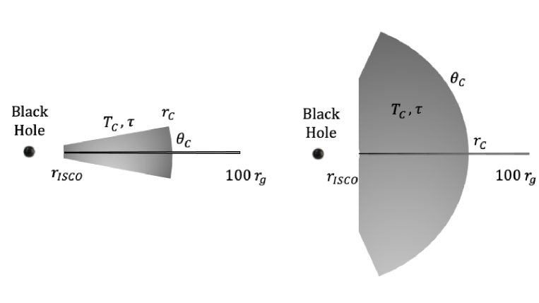
Figure 1: Sketches of simulated wedge-shaped coronae for a small and a large half opening angle $\theta_{C}$, left side and right side, respectively. The accretion disk extends from $r=r_{\rm ISCO}$ to $r=100\,r_{\rm g}$, and the corona with electron temperature $T_{C}$ and vertical optical depth $\tau_{C}$ extends from $r=r_{\rm ISCO}$ to $r=r_{C}$.

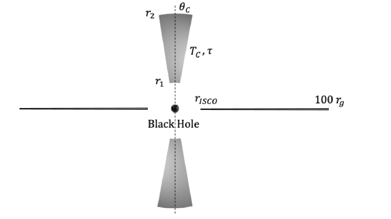
Figure 2: Sketch of simulated cone-shaped corona. The accretion disk extends from $r=r_{\rm ISCO}$ to $r=100\,r_{\rm g}$, and the corona with electron temperature $T_{C}$ and radial optical depth $\tau_{C}$ extends from $r=r_{1}$ to $r=r_{2}$ from the polar angle $\theta=0$ to $\theta=\theta_{C}$. The dashed line shows the black hole spin axis.

Corona electron temperatures $T_{\rm C}$ between 5 keV and 500 keV, and integrated optical depths between the case of no corona ($\tau_{\rm C}\,=\,0$) and $\tau_{\rm C}\,=\,2$ are simulated. For wedge-shaped coronae, the optical depth is measured vertically from the accretion disk to the upper (or lower) edge of the corona. For the cone-shaped coronae, the optical depth is measured radially from the inner to the outer edge of the corona. For a fast spinning black hole ($a=0.998$) with a wedge corona extending from the ISCO to $100\,r_{\rm g}$, the highest temperature ($T_{\rm C}=500$ keV), an optical depth perpendicular to the accretion disk of ($\tau_{\rm C}=2$), and a wedge angle of $20^{\circ}$, the code produces a power law component with a photon index $\Gamma$ (from $dN/dE\propto E^{-\Gamma}$) of $\sim$0.7.

The code tracks photons forward in time, and allows us to collect photons at arbitrary locations of the observer relative to the accreting system. A single simulation set can thus be used to infer the observations for all black hole inclination angles.

2.2 Raytracing Code

We generate the simulated energy spectra with the code xTrack described in (Krawczynski, 2012; Hoormann et al., 2016; Beheshtipour et al., 2017; Krawczynski et al., 2019; Abarr & Krawczynski, 2020a, 2021). We give here a slightly updated description of the code that includes several recent improvements.

The code uses the Kerr metric $g_{\mu\nu}$ in Boyer-Lindquist (BL) coordinates $x^{\mu}=(t,r,\theta,\phi)$. Photons are emitted and scatter in the reference frames of the emitting or scattering plasma, and are transported in the global BL coordinate frame. The reference frame transformations use orthonormal tetrads. The code assumes that the black hole accretes through a geometrically paper thin, optically thick accretion disk (Shakura & Sunyaev, 1973; Novikov & Thorne, 1973; Page & Thorne, 1974). For each black hole spin we calculate a fiducial temperature profile $T_{0}(r)$ with the accretion rate $\dot{M}$ chosen such that the luminosity

$$L_{\rm acc}\,=\,\eta(r_{\rm ISCO})\dot{M}$$ (1)

is 10% of the Eddington luminosity

$$L_{\rm Edd}\,=\,\frac{4\pi\,G\,M_{\rm BH}\,m_{\rm P}}{\sigma_{\rm T}}.$$ (2)

In the above equations, $\eta$ is the fraction of the gravitational energy of the matter that is converted to heat as the matter accretes from infinity to $r_{\rm ISCO}$ in units of the matter’s rest mass energy. The fraction is given by:

$$\eta(r_{\rm ISCO})\,=\,1-E^{\dagger}(r_{\rm ISCO})$$ (3)

with $E^{\dagger}(r_{\rm ISCO})$ being the specific energy at infinity of the matter at $r\,=\,r_{\rm ISCO}$:

$$E^{\dagger}\,=-\,g_{t\mu}\,u^{\mu}$$ (4)

where $g$ is the Kerr metric and $u^{\mu}$ the four velocity of the matter at the ISCO. Given the angular velocity $d\phi/dt=\Omega\,=\pm M^{1/2}/(r^{3/2}\pm aM^{1/2})$ (Bardeen et al., 1972), we get $u^{\mu}\,=\,u^{t}\,(1,0,0,\Omega)$ from the condition $u^{2}=-1$. The emissivity (power per comoving time and area) $F(r)$ is then given by Equations (11)-(12) of (Page & Thorne, 1974). We assume a fiducial temperature profile with

$$T_{0}(r)=\left(\frac{F(r)}{\sigma_{\rm SB}}\right)^{1/4},$$ (5)

where $\sigma_{\rm SB}$ is the Stefan Boltzmann constant. As mentioned above, we perform the simulations for a range of scaled temperature profiles:

$$T(r)\,=\,\sigma\,T_{0}(r)$$ (6)

with $\sigma$ between 0.05 and 2. We generate initial photon energies assuming a diluted blackbody energy spectrum with a hardening factor of $f_{\rm h}=1.8$ (Shimura & Takahara, 1995).

For each accretion disk and corona configuration, we simulate 2$\times$10⁷ photons, using 10,000 logarithmically spaced radial bins with $r$ running from $r_{\rm ISCO}$ to $100\,r_{\rm g}$. The photons are launched into the upper hemisphere with constant probability per solid angle with a limb brightening weighting factor and initial polarization given by Table XXIV of (Chandrasekhar, 1960). We normalize the limb brightening weighting factor so that the average weighting factor is 1.

An adaptive step-size Cash-Karp integrator based on a 5’th order Runge-Kutta algorithm is used to solve the geodesic equation, to update the the position ($x^{\mu}$), and the photon’s wavevector $k^{\mu}$, and to parallel transports the polarization vector $f^{\mu}$ (Abarr & Krawczynski, 2020a, b). The polarization fraction remains constant between scattering events. The step size is reduced if the traversed coronal optical depth evaluated in the rest frame of the corona exceeds 2% of the total optical depth of the corona. The step size is furthermore modified if the photon enters or leaves the corona, so that the end of the step coincides with the corona boundary.

Photons are tracked until their radial BL coordinate drops below 1.02 times the $r$-coordinate of the event horizon (at which point we assume that the photon will disappear into the black hole) or reach a fiducial observer at $r_{\rm obs}\,=$ 10,000 $r_{\rm g}$. In the latter case, the wave and polarization vectors are transformed into the reference system of a coordinate stationary observer, and key information is written to disk.

2.3 Calculation of Absolute Fluxes Reaching the Observer and Reaching the Accretion Disk

Each event is counted with a weighing factor that allows us to make absolute flux predictions. As mentioned above, the thin disk solution of Page & Thorne (1974) gives the plasma-frame energy flux $F(r)$ of the photons emitted at radius $r$. The number of photons emitted per Boyer-Lindquist $dt$, $dr$ and $d\phi$ is given by (Krawczynski, 2012):

$$\frac{dN}{dt\,dr\,d\phi}(r)\,=\,\frac{\sqrt{-g_{tr\phi}(r)}\,F(r)}{<\!E(r)\!>}$$ (7)

with $\sqrt{-g_{tr\phi}(r)}$ is the square root of the negative of $t-r-\phi$-part of the metric. For the Kerr metric, the factor simplifies to $\sqrt{-g_{tr\phi}(r)}=r$ in the equatorial plane. The mean plasma frame energy of the thermally emitted photons is given by

$$<\!E(r)\!>\,=\,2.7\,f_{\rm h}\,k_{\rm B}\,T_{\rm eff}(r).$$ (8)

Although Equation (7) has been derived from a relativistic invariant, the interpretation is simple: the photon flux per unit coordinate time $dN/dt$ equals the proper area-time volume element of the emitting disk segment $\sqrt{-g_{tr\phi}(r)}\,dr\,d\phi\,dt$ times the emitted energy flux per unit area $F(r)$ divided by the product of the mean energy of the emitted photons $<\!E(r)\!>$ times $dt$.

The $i$’th disk segment extending from $r_{i}-\Delta r_{i}/2$ to $r+\Delta r_{i}/2$ thus emits photons at a rate of:

$$\frac{dN_{i}}{dt}\,=\,\Delta r_{i}\,\int_{0}^{2\pi}\,d\phi\,\frac{dN}{dt\,dr\,d\phi}(r_{i})\,=\,2\pi\Delta r_{i}\,\frac{dN}{dt\,dr\,d\phi}(r_{i})$$ (9)

Given that we generate $N_{\rm bin}$ events per radial bin, each simulated photon transports the photon rate $\frac{dN_{i}}{dt}/N_{\rm bin}$. The photon rate per simulated event launched from the $i$’th bin is thus give by the weight:

$$w_{i}=\frac{1}{N_{\rm bin}}\frac{dN_{i}}{dt}=\frac{2\pi\,\sqrt{-g_{tr\phi}(r_{i})}\,\Delta r_{i}}{N_{\rm bin}}\frac{F(r_{i})}{<\!E(r_{i})\!>}$$ (10)

For a source at the distance $d$ from us, the flux spreads over an area:

$$A_{\Omega}\,=\,\Delta\Omega\,d^{2}$$ (11)

before reaching us. Here, $\Delta\Omega$ is the solid angle of the $\theta$-window that we use to collect the simulated photons. Each simulated event thus transports the photon flux:

$$f_{i}\,=\,\frac{1}{A_{\Omega}}w_{i}\,=\,\frac{2\pi\,\sqrt{-g_{tr\phi}(r_{i})}\,\Delta r_{i}}{N_{\rm bin}\,A_{\Omega}}\frac{F(r_{i})}{<\!E(r_{i})\!>}$$ (12)

per unit observer time and area. Differential photon fluxes per unit time, unit area, and unit energy (Stokes $I$, $Q$, and $U$) can be obtained by binning the results in observer energy and dividing the sum of all $f_{i}$ in each bin by the width of the energy bin.

The calculation of the reflected energy spectrum requires the knowledge of the flux and the photon index of the emission irradiating the $j$’th disk element. Tracing the argument that led to Equation (10) backwards, we infer that each event being launched from the $i$’th bin of width $\Delta r_{i}$ that reaches the $j$’th bin of width $\Delta r_{j}$ adds a plasma frame energy flux of

$$f_{i\rightarrow j} = \frac{E_{d}\,w_{i}}{2\pi\sqrt{-g_{tr\phi}(r_{j})}\,\Delta r_{j}}$$ (13)

$$= \frac{F(r_{i})}{N_{\rm bin}}\frac{\sqrt{-g_{tr\phi}(r_{i})}\Delta r_{i}}{\sqrt{-g_{tr\phi}(r_{j})}\Delta r_{j}}\frac{E_{d}}{<E_{i}>}$$

to the energy flux irradiating the bin. Here, $E_{d}$ is the plasma frame energy of the photon irradiating the disk. This equation has again a simple interpretation: the energy flux transported by each event starting at bin $i$ and reaching bin $j$ is the energy flux $F(r_{i})$ leaving bin $i$ divided by the number of events launched from the $i$’th bin times the ratio of the area-time volumes of the $i$’th and $j$’th radial bins times the fractional energy gain or loss of the photon between emission from bin $i$ and arrival at bin $j$.

Summing $f_{i\rightarrow j}$ over all events irradiating the $j$’th radial bin gives the total plasma frame energy flux $F_{x}(r_{j})$ irradiating the bin. Reflections off the disk and/or Compton scattering processes modify the statistical weight of a photon.

In a photospheric plasma with comoving electron density $n_{\rm e}$ (Ross & Fabian, 1993; Ross et al., 1996; Ross & Fabian, 1996; Ross et al., 1999), the ionization can be characterized with the ionization parameter $\xi$. The parameter is proportional to the ratio of the photoionization rate ($\propto n_{\rm e}$) divided by the recombination rate ($\propto n_{\rm e}^{\,2}$):

$$\xi(r_{j})=\frac{4\pi F_{x}(r_{j})}{n_{\rm e}(r_{j})}.$$ (14)

The energy spectra of all photons arriving in the radial bin $j$ can be used to fit the photon index $\Gamma_{j}$ (from $dN/dE\propto E^{-\Gamma}$) of the emission irradiating the bin.

A limitation of our code should be mentioned: photons reflecting off the disk more than once are not modeled fully self-consistently. For these photons, only their first encounter with the disk contributes to the calculation of $\xi$ and $\Gamma$, and additional encounters are neglected. The statistical weight of the subsequent photon-disk encounters depends on the $\xi$ and $\Gamma$ values used for the previous encounters. Properly accounting for multiple disk-photon interactions would thus render the problem non-linear. For the purpose of calculating the predicted energy spectra, kerrC does track the photons through multiple disk encounters. However, the XILLVER tables are only used to modify their statistical weight for their first disk encounter. For subsequent encounters, the weights from the Chandrasekhar treatment are used. We estimated the impact of these approximations on the fitted parameters, by using the “opposite” assumptions, i.e. by including the additional photon-disk encounters in the $\xi$ and $\Gamma$ calculation with their full Chandrasekhar weight, and by completely excluding photons scattering more than once from entering the predicted energy spectra. We find that the approximations have a negligible impact in case of the cone-shaped corona models as few photons return multiple times to the disk. Adopting the alternative assumptions for the wedge-shaped coronae tends to harden the energy spectra impinging on the disk for the high-$\xi$ models and to soften the predicted energy spectra for the low-$\xi$ models. We will explore the problem and possible solutions in greater detail in future papers.

2.4 Comptonization

We use the Comptonization code of (Beheshtipour et al., 2017; Beheshtipour, 2018). The coronal plasma is assumed to be stationary in the Zero Angular Momentum Observer (ZAMO) frame (Bardeen et al., 1972). See (Krawczynski, 2021) for a formalism to implement relativistically moving coronal gas. For each integration step, the traversed Thomson optical depth $\Delta\tau$ is calculated and a random number generator decides if the photon is considered for a coronal scattering event. The scattering event is simulated by transforming the photon’s wave and polarization four vectors into the ZAMO frame, and subsequently into the frame of a scattering electron. We assume that electrons move isotropically in the ZAMO frame with energies drawn from a relativistic Maxwell–Jüttner distribution (Jüttner, 1911). The scattered photon direction is drawn from a distribution with equal scattering probability in the electron rest frame. Subsequently, the Stokes parameters are calculated relative to the scattering plane. The fully relativistic Fano scattering matrix derived from the Klein-Nishina cross section (Fano, 1949; McMaster, 1961) is used to calculate the Stokes vector of the outgoing beam. We use the Stokes $I$ component of the scattered beam and a random number generator to decide if a photon actually scatters. This rejection technique enables us to account for the dependence of the scattering probability on the scattering direction and on the photon energy. If the photon indeed scatters, the statistical weight is multiplied with the kinematic factor $1-\cos{(\theta)}$ with $\theta$ being the pitch angle of the incoming photon and electron, accounting for the relative motion of the photons and electrons (Beheshtipour et al., 2017). The scattering is followed by the back transformation of the photon wave and polarization vectors into the BL frame.

2.5 Preliminary Disk Reflection

For photons irradiating the accretion disk, we perform a simple reflection in the reference frame of the disk plasma based on the analytical results of Chandrasekhar for the reflection of a polarized beam of photons off an indefinitely deep plane-parallel atmosphere (Chandrasekhar, 1960, Section 70.3, Equation (164) and Table XXV). The reflection changes the statistical weight of the reflected beam, and the linear polarization fraction and angle. For each reflected photon, the code saves information about the incident photon and the reflected photon as measured in the disk reference frame, and information about the photon when it reaches the observer. This information is used during the actual fitting of the observational data to re-weigh the reflected photons, so that the reflected energy spectrum resembles that from the XILLVER radiation transport calculations for the self-consistently derived ionization parameter $\xi(r)$ and the spectral index $\Gamma(r)$ of the emission irradiating the accretion disk.

3 Implementation of the kerrC Model

3.1 Implementation Details

The kerrC fitting model uses a data bank of 1.36 trillion simulated events (20 million events for each of the 68,040 configurations.) The raytracing code stores for this purpose three types of data: data of photons reaching the observer without reflecting off the disk (direct emission data), data of photons irradiating the disk (disk data), and data of photons reaching the observer after scattering at least once off the accretion disk (reflected emission data). This classification is independent of the scattering of photons in the corona. The data are stored in Hierarchical Data Format version 5 (HDF5) files which makes it possible to quickly access the information of the photons that matter for the considered region of the parameter space.

Table 2: kerrc model parameters

Number	Parameter	Symbol	KerrC name	Unit	Allowed Values
Black Hole Parameters
1	Black Hole Mass	$M$	M	$M_{\odot}$	any
2	Black Hole Spin Parameter	$a$	a	none	-1 … 0.998
3	Black Hole Inclination	$i$	incl	degree	5 … 85
4	Distance	d	dist	kpc	0 … $\infty$
Accretion Flow Parameters
5	Mass Accretion Rate	$\dot{M}$	mDot	$10^{18}\,{\rm g\,s}^{-1}$	depend on $M$
Corona Parameters
6	Corona Geometry	$g$	geom	none	0, 1
7	Corona Edgea	$r_{\rm C}$	rC	$r_{\rm g}$	2.5 … 100
8	Corona Opening Angle	$\theta_{\rm C}$	thetaC	degree	5 … 85
9	Corona Temperature	$kT_{\rm C}$	tempC	keV	5 … 100
10	Corona Optical Depth	$\tau_{\rm C}$	tauC	none	0 … 2
Reflection Parameters
11	Reflection Amplitudeb	-	refl	none	0 … 10
12	Metallicity	$A_{Fe}$	AFe	solar	0.5-10
13	Electron Temp.	$kT_{\rm e}$	kTe	keV	1-400
14	Electron Density at $r_{\rm ISCO}$	log${}_{10}\,n_{\rm e,0}$	logDens	cgs	15-22
15	Radial Density Powerlaw Index	$\alpha$	xiIndex	none	0 …
16	$\Gamma$-fit rangec	$\kappa$	kappa	none	0.1…10
Polarization Parameters
16	Angle of BH Spin Axes from Cel. North Pole, counter-clockwise	$\chi$	chi	degree	0 … 180
Additional Model Modifiers
17	Inner Cutoffd	$l_{1}$	l1	$r_{\rm g}$	0, $r_{\rm ISCO}$ … 100
18	Outer Cutoffd	$l_{2}$	l2	$r_{\rm g}$	0, $r_{\rm ISCO}$ … 100

^a The corona edge parameter gives the outer edge of the wedge-shaped corona (25 … 100 $r_{\rm g}$) and the inner edge of the cone-shaped corona (2.5 … 50 $r_{\rm g}$).
^b The reflection amplitude should be set to unity to get the self-consistently calculated reflection.
^c XILLVER requires the photon indices of the emission irradiating the accretion disk. We fit the energy spectra from $\kappa E_{1}$ to $\kappa E_{2}$ with $\kappa\,=\,1.5$, $E_{1}\,=\,1$ keV and $E_{2}\,=\,10$ keV.
^d $l_{1}$ ($l_{2}$) give a lower (upper) bound on the radial coordinate of the emission of photons entering the analysis.

The fitting code is implemented as a user model for the Sherpa fitting package (Freeman et al., 2001; Doe et al., 2007; Refsdal et al., 2009; Brian Refsdal et al., 2011). While the user model uses a Python interface, the work of reading and convolving the raytraced photon and the reflection model data, and interpolating between the simulated grid points is done by a fast C++ code compiled into a Python module with the help of the Boost-Python library (D. Abrahams and R. W. Grosse-Kunstleve) of the Boost distribution.

3.2 Fitting Parameters

The KerrC model parameter are listed in Table 2. The parameters include the black hole mass $M$, the black hole spin $a$, black hole inclination $i$, and distance $d$. The accretion flow is characterized by a single parameter, the mass accretion rate $\dot{M}$. The model parameter $g$ selects between the wedge-shaped and cone-shaped corona configurations characterized by $r_{C}$, $\theta_{C}$, $T_{C}$, and $\tau_{C}$ as described above.

The reflection parameters include an amplitude to increase the reflected emission above or below the self-consistently derived intensity. The other reflection parameters describe the physical conditions in the photosphere of the accretion disk. The parameters include the metallicity $A_{Fe}$ relative to solar, the electron density $n_{\rm e}$ at the inner edge of the accretion disk, and a power law index giving how the electron density scales with radial distance ($n(r)\propto r^{-\alpha}$). XILLVER assumes that the photons irradiating the accretion disk have an energy spectrum of disk photons comptonized by electrons of temperature $kT_{\rm e}$ according to the Nthcomp model (Zdziarski et al., 1996; Życki et al., 1999). We consider $kT_{\rm e}$ as a free fitting parameter here. The parameter $\kappa$ modifies the energy range used for determining the photon index of the emission irradiating the disk. We use $\kappa=1.5$ giving a fitting range from 1.5 keV to 15 keV. As mentioned above, the code calculates all three Stokes parameters. The model parameter $\chi$ gives the rotation of the black hole spin axis of the model relative to the celestial north pole (the black hole spin axis of the model is turned counter-clockwise for $\chi>0$). Finally, the user can exclude photons launched at radial distances outside the $l_{1}$ … $l_{2}$ interval from the analysis. This can be used to estimate the impact of disk truncation or shadowing in rough approximation.

3.3 Model Evaluation

As described above, we simulated a library for a set of black hole, accretion disk, and corona configurations. When kerrC is called with parameters between the simulated ones, kerrC identifies the nearby simulated configuration nodes, calculates energy spectra for these nodes, and returns an interpolated energy spectrum using linear interpolation in simplices (Weiser & Zarantonello, 1988).

For each configuration node, the direct emission data are used to calculate the energy spectrum of the direct emission. Subsequently, the disk data are analyzed to obtain the radial 0.1-1000 keV fluxes $f_{i}$ and the 1.5-15 keV photon indices $\Gamma_{i}$ of the returning and corona photons irradiating the disk in logarithmicly spaced radial bins ($i=1...12$). For the same radial bins, the plasma frame energy spectra $F_{C,i,j}(E)$ of photons scattered into each of 10 inclination bins ($j=1...10$) are acquired. The inclination refers to the plasma frame direction of the scattered photon. The subscript $C$ indicates that these energy spectra are based on Chandrasekhar’s scattering formalism.

In the last step, the reflected energy spectra are calculated. For this purpose, each reflected photon enters the analysis with a weight that accounts for the results from the XILLVER radiative transport calculations. We use the energy spectra $F_{X}(\Gamma,A_{Fe},\log_{10}\xi,kT_{\rm e},\log_{10}n_{\rm e},\theta;E)$ from the XILLVER tables version Cp_3.6 . Here, $\Gamma$ is the photon index of the emission irradiating the accretion disk, $A_{Fe}$ is the metallicity relative to solar system metallicities, $\xi$ is the ionization parameter, $kT_{\rm e}$ is the electron temperature describing the Comptonized XILLVER input energy spectrum, $n_{\rm e}$ is the electron density of the reflecting plasma, $\theta$ is the plasma frame inclination angle of the reflected emission, and $E$ is the plasma frame energy of the incoming and outgoing photon.

Our treatment seeks to minimize the impact of the XILLVER input energy spectra by multiplying each photon’s statistical weight with the ratio $r$ of the energy spectrum for the actual ionization parameter divided by the energy spectrum for the highest simulated ionization parameter ($\log_{10}\xi_{\rm max}=4.7$):

$$r\,=\,\frac{F_{X}(\Gamma_{i},A_{Fe},\xi(r_{i}),kT_{\rm e},n_{\rm e}(r_{i}),\theta;E)}{F_{X}(\Gamma_{i},A_{Fe},\xi_{\rm max},kT_{\rm e},n_{\rm e}(r_{i}),\theta;E)}$$ (15)

The index $i$ denotes the radial bin $r_{i}$ where the reflection takes place, $\Gamma_{i}$ and $\xi(r_{i})$ are known from the disk analysis, $kT_{\rm e}$ is a fit parameter, $n_{\rm e}(r_{i})$ follows from the fit parameters $n_{\rm e,0}$ and $\alpha$, and $\theta$ and $E$ are the inclination and energy of the reflected photon. The multiplicative correction is justified by the fact that the XILLVER results for $(\log_{10}\xi)_{\rm max}=4.7$ agree with Chandrasekhar’s results for a pure electron scattering atmosphere (Garcia, 2010, and private communication). The motivation for our treatment is that the reflected Chandrasekhar energy spectrum resembles the reflected energy spectrum to first approximation. The re-weighting factor is used as a correction of the Chandrasekhar result. The treatment leads to more physical results than using the ratio of the XILLVER energy spectrum divided by the incident energy spectrum. In the latter case, the XILLVER assumption of incident power law energy spectra can lead to reflected energy spectra with unphysically high fluxes of high-energy photons, exceeding by far the high-energy photon fluxes provided by the corona. The XILLVER tables are binned in 2999 logarithmicly spaced energy bins from 0.07 to 1000.1 keV (adjacent bins spaced 0.3% apart). We smooth the XILLVER results with a Gaussian kernel with a $\sigma$ of 6 bins (1.9%) to reduce statistical errors associated with a poor sampling of the XILLVER tables by the simulated photons.

Although our reflection treatment conserves the plasma frame photon energy for each individual photon, the reweighing with the XILLVER results accounts for energy gains and losses when averaged over many photons. The code uses linear interpolation in simplices to get the XILLVER energy spectra between the simulated XILLVER nodes. If we hit the edge of the simulated parameter space, we use the edge value.

Our code uses Chandrasekhar’s results for the polarization of photons scattering off an indefinitely deep electron atmosphere. For each reflection of a photon, the result accounts for the polarization fraction and direction and the inclination and azimuth angles of the incoming and outgoing photon beams. The polarization treatment is thus rather detailed, but neglects the impact of atomic emission and absorption. As scattering tends to generate polarization, but atomic emission does not, our predicted Fe K-$\alpha$ polarizations are expected to be slightly too high. The treatment furthermore does not account for the difference of the polarization dependence between the Thomson and Klein-Nishina scattering cross sections.

Some XILLVER models did not converge satisfactorily (J. García, private communication). For electron densities $n_{\rm e}>10^{19}$ cm^-3 we thus use the XILLVER model for $n_{\rm e}=10^{19}\,\rm cm^{-3}$.

The code saves CPU time by storing and later re-using some of the intermediate results. For example, as long as $l_{1}$ and $l_{2}$ are not changed, the direct emission results and the disk analysis results can be stored and re-used for each configuration node. The reflected emission results need to be re-calculated every time the reflection parameters are changed.

Figure 3: Comparison of kerrC (orange lines) and KERRBB (blue lines) (Li et al., 2005). Panel (a) shows the models for a spin $a$ of 0.98, inclinations $i$ of $27.51^{\circ}$ (left) and $65^{\circ}$ (right), a black hole mass of 21.2 $M_{\odot}$, an accretion rate $\dot{M}$ of 0.17$\times 10^{18}$ g/sec, a source distance of 2.22 kpc, a hardening factor of 1.8, reflected returning emission switched off, and with limb brightening. The other three panels compare the two models for the $i\,=\,27.51^{\circ}$ case of (a) when one of the parameters is changed but all others are held constant, i.e. when the black hole mass is decreased to 15 $M_{\odot}$ (b), when $\dot{M}$ is increased to 0.5$\times 10^{18}$ g/sec (c), and when the spin parameter $a$ is reduced to 0.75 (d).

3.4 Scaling Relations

The thin disk solution of Page & Thorne (1974) implies the following scaling relations of the temperature scale $\sigma$, the observer flux multiplier $f_{i}$, and the disk flux multiplier $f_{i\rightarrow j}$ with black hole mass $M$, mass accretion rate $\dot{M}$, and source distance $d$:

$$\sigma \propto M^{-1/2}\,\dot{M}^{1/4}$$ (16)

$$f_{i} \propto M^{1/2}\,\dot{M}^{3/4}\,d^{-2}$$ (17)

$$f_{i\rightarrow j} \propto M^{-3/2}\,\dot{M}^{3/4}.$$ (18)

We extracted these scaling relations by numerically calculating the temperatures and weighting factors for different $M$ and $\dot{M}$ input parameters, and evaluating how they depend on these input parameters. kerrC uses Equation (16) to map the $M$ and $\dot{M}$ values provided by the user to a temperature scale $\sigma$, and then uses this $\sigma$ to interpolate between the simulated $\sigma$-values. Equations (17) and (18) are used to adjust the flux multipliers in the analyses of the direct emission, the emission irradiating the disk, and the reflected emission.

3.5 Code Validation

We validate KerrC by comparing the predictions for the thermal energy spectrum with the results of KERRBB (Li et al., 2005). Figure 3 shows that the comparison of the kerrC and KERRBB energy spectra typically agree within $<\sim$20%. The most pronounced differences can be recognized at energies below 0.5 keV. The fact that kerrC underpredicts those fluxes can be explained by the fact that it only accounts for the emission from $r\leq 100\,r_{\rm g}$. At larger radial distances, the accretion disk emits at rather low energies. Some additional differences may stem from KERRBB using a limb brightening proportional to $1+\cos{(\theta)}$ and kerrC using the limb brightening prescription from Chandrasekhar’s indefinitely deep electron scattering atmosphere. Overall, the energy spectra of the two codes agree well.

We have validated the flux energy spectrum and polarization energy spectrum of kerrC with that of the code MONK (Zhang et al., 2019) and found excellent agreement (Zhang et al., private communication).

4 Fit of intermediate-state Cyg X-1 data with kerrC

We show here results from using kerrC to fit the NuSTAR (Harrison et al., 2013) and Suzaku (Mitsuda et al., 2007) observations of the archetypical black hole Cyg X-1 in the intermediate state. The data were acquired on May 27-28, 2015 and include 19,860 sec and 20,500 sec of NuSTAR Focal Plane Module A and B observations, respectively. We analyzed the data with the NuSTARDAS analysis pipeline provided with the software package HEAsoft 6.28. We use furthermore 4,991 sec of Suzaku data aquired with the X-ray Imaging Spectrometer #1 (XIS1 Koyama et al., 2007) on the same days. The NuSTAR and Suzaku data have been published in (Tomsick et al., 2018). The authors kindly shared the Suzaku XIS1 data with us. We only use the 3-20 keV NuSTAR data, as the statistical errors of the kerrC model become appreciable above this energy. Following Tomsick et al. (2018), we use only the 1-1.7 keV and 2.1-8 keV Suzaku XIS1 data.

Table 3: Best-fit wedge-shaped corona model.

Parameter	thawed?	Result (90% CL uncertainty)
Absorption
$n_{\rm H}$	frozen	0.6$\times 10^{22}$ cm-2
Black Hole Parameters
$M$	frozen	21.2 $M_{\odot}$
$a$	thawed	0.861
$i$	frozen	27.51∘
$d$	frozen	2.22 kpc
Accretion Flow Parameters
$\dot{M}$	thawed	0.158$\times 10^{18}\,{\rm g\,s}^{-1}$
$r_{\rm C}$	thawed	72.9 $r_{\rm g}$
$\theta_{\rm C}$	thawed	21.8∘
$kT_{\rm C}$	thawed	100 keV
$\tau_{\rm C}$	thawed	0.256
Reflection Parameters
$A_{Fe}$	frozen	1 solar
$kT_{\rm e}$	thawed	1 keV
$\log_{10}n_{e,0}$	thawed	20.8
Other Parameters
$\alpha$	frozen	0
$l_{1}$	frozen	$r_{\rm ISCO}$
$l_{2}$	frozen	$100\,r_{\rm g}$
Fit Statistics
$\chi^{2}/$DoF	NA	7136/1582

The estimates of the distance and mass of Cyg X-1 have recently been revised Miller-Jones et al. (2021). The new distance estimate accounts for the impact of an orbital phase dependent attenuation of the radio signal, and localizes the source at a distance of $d\,=$ (2.22+0.18-0.17) kpc. The revised distance and optical data constrain the black hole mass to be $M\,=$ 21.2$\pm$2.2 $M_{\odot}$. The orbital plane inclination is $27.51^{\circ}$ with 68% confidence level lower and upper bounds of 26.94^∘ and 28.28^∘.

We fit the kerrC model absorbed with a fixed $n_{H}=0.6\times 10^{21}$ (Tomsick et al., 2018) with the cross sections of Verner et al. (1996) and the elemental abundances of Wilms et al. (2000). We freeze $M$, $d$, $i$, and $n_{\rm H}$, and assume an accretion disk plasma with solar elemental abundances ($A_{Fe}\,=\,1$).

We fit the kerrC parameters $\dot{M}$, $r_{\rm C}$, $\theta_{\rm C}$, $kT_{\rm C}$, $\tau_{\rm C}$ and $\log_{10}n_{\rm e}$. We assume that the electron density of the photosphere does not depend on the radial coordinate ($\alpha\,=\,0$), and we do not investigate the impact of a truncated or shadowed disk. We fitted the data by first evaluating the model at all simulated configuration nodes for one particular set of XILLVER parameters. Subsequently, we started the fitting with Sherpa from the configuration node with the smallest $\chi^{2}$-value. We got the smallest $\chi^{2}$-values by randomly thawing four parameters at a time and repeating the fit, switching between the levmar and moncar minimization engines. We ran the minimization many times with different starting values. A good number of fits gets stuck in local minima.

A wedge-shaped corona gives the best fit with a $\chi^{2}$ of 7136 for 1582 degrees of freedom (DoF). The best cone-shaped corona gives a $\chi^{2}/$DoF of 8001$/$1582. In the following, we discuss the results for the two corona models in turn. The $\chi^{2}$/DoF-values are significantly larger than unity showing that systematic rather than statistical errors dominate the error budget. We thus refrain from giving statistical error estimates. A detailed error analysis is outside of the scope of this paper.

4.1 The Best-Fit Wedge-Shaped Corona Model

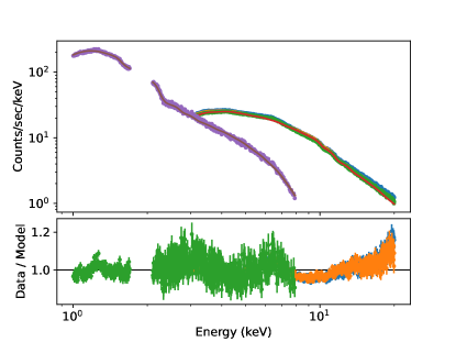
Figure 4: Cyg X-1 Suzaku (blue data points), NuSTAR (green and orange data points) data with the best-fit wedge-shaped corona model (lines). The top panel shows the detection rate, and the lower panel the ratio of the observed count rate divided by the modeled count rate.

Figure 5: kerrC results for one of the configuration nodes of the best-fitting wedge-shaped corona model shown in Fig. 4 ($a\,=\,0.9$, $T_{\rm C}\,=\,100$ keV, $\tau_{\rm C}\,=\,0.5$, $\theta_{\rm C}\,=\,45^{\circ}$, and $r_{\rm C}\,=\,100\,r_{\rm g}$). (a) Thermal and coronal flux and reflected flux; (b) 0.1-1000 keV plasma frame flux of the thermal disk emission (orange dotted line), the returning emission irradiating the disk (dashed green line), and the returning and coronal emission (solid blue line); (c) 1.5-15 keV photon indices of the emission irradiating the accretion disk; (d) ionization parameter. (e) plasma frame energy spectra of the returning and coronal emission irradiating the accretion disk for 12 radial bins with bin centers ranging from $r\,=\,2.3\,r_{\rm g}$ (thinnest line) to $73\,r_{\rm g}$ (thickest line). (f): same as (e) but multiplied with the correction factor $r$ from Equation (15) for the inclination of emission $\theta\,=\,41.4^{\circ}$. These energy spectra show the shape of the reflected energy spectra. kerrC chooses for each individual photon the correction factor $r$ according to the photon’s reflection angle.

The parameters of the best-fit wedge-shaped corona are listed in Table 3. The model has a modest black hole spin of $a=0.861$, lower than the previously published values from the fitting of the thermal state $a\,>\,0.9985$ (Miller-Jones et al., 2021) and from similarly high values from fitting of the broadened Fe K-$\alpha$ line shapes (Tomsick et al., 2014; Duro et al., 2016; Walton et al., 2016; Tomsick et al., 2018).

The wedge-shaped corona has a half opening angle of 21.8^∘ and extends from the ISCO at $r_{\rm ISCO}\,=\,2.87$ $r_{\rm g}$ to 72.9 $r_{\rm g}$. The corona temperature is 100 keV and the optical depth is 0.256. The photospheric electron density is $\log_{10}{n_{\rm e}}\,=\,$20.8. The XILLVER electron temperature goes to the lowest possible value, indicating that the fit prefers reflection energy spectra predicted for soft energy spectra irradiating the accretion disk.

Figure 4 compares the best fit with the Suzaku and NuSTAR data. Overall, the agreement is typically good to a few percent. The modeled 1-1.7 keV energy spectrum is missing a peak in the middle of this energy range. Furthermore, the model does not fully reproduce the Fe K-$\alpha$ peak around 6.4 keV, and is too soft at $>$15 keV.

Figure 5 gives some of the internal kerrC results for the first configuration node chosen by the interpolation engine ($a\,=\,0.9$, $T_{\rm C}\,=\,100$ keV, $\tau_{\rm C}\,=\,0.5$, $\theta_{\rm C}\,=\,45^{\circ}$, and $r_{\rm C}\,=\,100\,r_{\rm g}$). This node usually impacts the results most strongly. Panel (a) shows the emission that did not experienced a reflection (blue) and the emission reflected at least once (orange). Both of these components may or may not have experience one or several Compton scatterings in the corona. The reflected emission starts to dominate at and above 8 keV. Around $\sim$1 keV, the flux without reflection is almost one order of magnitude stronger than the reflected emission. Panel (b) shows the disk frame thermal emission from the disk (dotted orange line), the returning emission (dashed green line), and the returning and coronal emission (blue solid line). The dashed green line was calculated for the same accretion disk without a corona. Two interesting conclusions: (i) the thermal flux from the disk approximately equals the coronal flux. Some of the accretion disk photons are energized (Comptonized) in the corona, and come back, giving rise to a coronal energy flux similar to the original accretion disk energy flux; (ii) the photons returning to the disk owing to spacetime curvature alone (without scattering in the corona), make up only a small fraction of the energy flux irradiating the disk. Panel (c) presents the 1.5-15 keV photon indices of the photons irradiating the accretion disk, showing a graduate steepening further away from the black hole. The ionization drops from $\log_{10}{\xi}$ $\sim$2 close to the ISCO to $\log_{10}{\xi}$ $\sim$0 at 100 $r_{\rm g}$. Finally, the last two panels show the comoving energy spectra of the photons irradiating the disk (Panel (e)) and the emission leaving the disk (Panel (f)) for different radial bins (see the Figure caption for additional details). Interestingly, the fit does not choose a combination of higher $n_{\rm e}$ and lower $\xi$ (which would give more pronounced lines), as the overall shape of the energy spectrum does not fit well for lower $\xi$-values.

4.2 The Best-Fit Cone-Shaped Corona Model

The parameters of the best-fit cone-shaped corona are listed in Table 4. This model has a slightly higher black hole spin of $a=0.921$ with an innermost stable circular orbit at $r_{\rm ISCO}\,=\,2.17\,r_{\rm g}$. The corona is rather distant from the black hole and extends from 41.4 $r_{\rm g}$ to 89.3 $r_{\rm g}$. The opening angle is found at the largest simulated value of 45 ^∘. Overall, the corona is thus far away and rather extended. The optical depth of the corona is with 0.64 larger than in the case of the wedge-shaped corona (0.256), probably to provide the disk with a sufficiently large flux even though the corona is rather distant and lets a good number of photons escape without scattering. The coronal temperature is with 107 keV slightly higher than in the case of the wedge-shaped corona (100 keV). The photospheric electron density is $\log_{10}{n_{\rm e}}\,=\,16.3$, much lower than in the case of the wedge-shaped corona. The XILLVER electron temperature is 50 keV. Similar as for the wedge-shaped corona, the model fits the data within a few percent for most of the range with larger deviations in the 1-1.7 keV energy range, around 6.4 keV, and at the highest energies (Fig. 6).

Table 4: Best-fit cone-shaped corona model. Only thawed parameters are listed; see Table 3 for frozen parameters (including $n_{\rm H}$).

Parameter	Result (90% CL uncertainty)
Black Hole Parameters
$a$	0.921
Accretion Flow Parameters
$\dot{M}$	0.167$\times 10^{18}\,{\rm g\,s}^{-1}$
Corona radial extent	41.4 $r_{\rm g}$-89.3 $r_{\rm g}$
$\theta_{\rm C}$	45∘
$kT_{\rm C}$	107 keV
$\tau_{\rm C}$	0.64
Reflection Parameters
$kT_{\rm e}$	50 keV
$\log_{10}n_{e,0}$	16.3
Fit Statistics
$\chi^{2}/$DoF	8001/1582

Figure 7 shows detailed information for the first interpolation node ($a\,=\,0.95$, $T_{\rm C}\,=\,250$ keV, $\tau_{\rm C}\,=\,0.75$, $\theta_{\rm C}\,=\,45^{\circ}$, $r_{1}\,=\,50\,r_{\rm g}$, and $r_{2}\,=\,100\,r_{\rm g}$). Panel (a) shows that the reflected energy spectrum starts to dominate over the non-scattered disk and coronal emission at much lower energies, i.e. around 2.5 keV. Panel (b) shows that the corona illuminates the accretion disk weakly at $r\sim r_{\rm ISCO}$, where the returning thermal emission dominates the disk illumination. The coronal Comptonized emission starts to dominate the disk illumination above $\sim$5 keV. Panel (c) presents the photon indices of the emission irradiating the disk. The energy spectra soften up to $\sim$4 $r_{\rm g}$ where the returning emission dominates and harden at larger distances, where the coronal emission dominates. Panel (d) shows the resulting ionization parameter of the disk plasma. The pronounced minimum at $\sim 10\,r_{\rm g}$ results from the combination of the strong evolution of the energy spectrum as a function of the distance from the black hole and the transition from the dominance of the returning radiation to the dominance of the coronal emission. Panel (e) shows how the energy spectra harden with distance from the black hole as the coronal emission gains importance. Panel (f) shows that the reflected energy spectra are almost featureless close to the black hole and only show emission lines for the outermost radial disk bins.

The results indicate that cone-shaped coronae have difficulties Comptonizing a sufficiently large fraction of the accretion disk photons to account for the observed power law emission. The best-fit corona thus resembles a large umbrella-shaped corona with a large opening angle, enabling it to Comptonize a large fraction of the accretion disk photons. The fit chooses furthermore a low electron density and thus a very high disk ionization which leads to a high-yield of the reflected emission. This result for the stellar mass black hole Cyg X-1 somewhat resembles similar difficulties in some Active Galactic Nuclei (AGNs) where compact coronae close to their black holes cannot explain the observed high reflected fluxes (Dovčiak & Done, 2016).

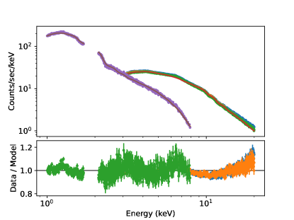
Figure 6: Same as Fig. 4 but for the best-fitting cone-shaped corona model.

Figure 7: Same as Fig. 5, but for one of the configuration nodes of the best-fitting cone-shaped corona model ($a\,=\,0.95$, $T_{\rm C}\,=\,250$ keV, $\tau_{\rm C}\,=\,0.75$, $\theta_{\rm C}\,=\,45^{\circ}$, $r_{1}\,=\,50\,r_{\rm g}$, and $r_{2}\,=\,100\,r_{\rm g}$).

Figure 8: Predicted $I$, $Q$, and $U$ energy spectra (top), polarization fractions (center), and polarization angles (bottom) for the best-fit wedge-shaped corona model (a) and the best-fit cone-shaped corona model (b). Positive (electric field) polarization angles are measured counter-clockwise from the block hole spin axis. We are looking from above at an accretion disk rotating according to the right hand rule with the black hole spin pointing upwards.

Figure 9: Simulated outcomes of a 500 ksec IXPE observation of Cyg X-1 for the best-fit wedge model (a,c) and the best-fit cone model (b,d). The upper panels show Stokes $I$ and the lower panels show Stokes $Q/I$ and $U/I$. For Stokes $Q/I=1$ and $U/I=0$, the electric field of the X-ray emission is parallel to the black hole angular momentum vector; for Stokes $Q/I=0$ and $U/I=1$, it is 45^∘ rotated counter-clockwise.

5 Predicted IXPE Results

We developed a code to simulate and fit IXPE observations for any model available in Sherpa, including kerrC. Sherpa and X-Spec user will know the fake command used to combine a model with response matrices to generate simulated energy spectra. Along similar lines, we added a Python object simPol that provides a fake method to generate Stokes $Q$ and Stokes $U$ energy spectra.

The code requires the model of the $I$, $Q$, and $U$ energy spectra, the Ancillary Response File (ARFs) (effective detection area as a function of energy), the Response Matrix Files (RMFs) (energy redistribution owing to detection principle and detector effects), and the Modulated Response File (MRF). The MRF is the ARF times the energy-dependent modulation factor $\mu(E)$. The modulation factor gives the fractional modulation of the reconstructed polarization directions for a 100% polarized signal and depends on the polarimeter performance, and the event reconstruction methods.

The analysis of X-ray polarization data is based on assigning each detected X-ray photon a Stokes parameter $i=1$,$q\,=\frac{2}{\mu(E)}\cos{(2\psi)}$ and $u\,=\frac{2}{\mu(E)}\sin{(2\psi)}$ with $\psi$ being the reconstructed polarization direction and $E$ the reconstructed energy of the event (Kislat et al., 2015; Strohmayer, 2017). The sums $I$, $Q$, and $U$ of the $i$, $q$ and $u$ values of all events, respectively, are binned in energy and form the basis of the analysis. The data are then analyzed by simultaneously fitting the detected and modeled $I$, $Q$ and $U$ energy spectra, using the uncertainties $\sqrt{I}$ on $I$, and $\sqrt{2I}/\mu$ on $Q$ and $U$. The simPol fake method uses the $Q$ and $U$ standard deviations and $Q$-$U$ covariances to generate observed $Q$ and $U$ energy spectra Kislat et al. (2015). Polarization fractions $p$ and directions $\chi$ can be calculated from $p\,=\,\sqrt{Q^{2}+U^{2}}/I$ and $\psi\,=\,\frac{1}{2}{\rm arctan2}(U,Q)$. We use the preliminary IXPE ARFs, RMFs, and MRFs from Baldini (2020), and show in the following only the results summed over all three IXPE detectors.

Figure 8 presents the polarization energy spectra for the two best-fit models for a simulated 500 ksec IXPE observation of Cyg X-1. The predicted polarization fractions turn out to be rather low for the two models: lower than 1% below 4 keV and about 1% at and above 4 keV. The $>$4 keV polarization fractions is higher for the wedge-shaped corona than for the cone-shaped corona. In the 4-6 keV energy range the expected polarization directions are parallel to the black hole spin axis. For polarization fractions $<1\%$, the statistical errors on the predicted $Q$ and $U$ values are not entirely negligible.

The differences between $Q/I$ and $U/I$ energy spectra of the two models come from the different black hole spins, the different polarizations that the photons acquire in the coronae of different shapes, and from the different accretion disk irradiation and reflection patterns. Note that the reflected intensity depends among other factors strongly on $\xi(r)$, which are very different for the two corona models.

Figure 9 shows the simulated IXPE results for the two coronae. For both corona models, the detection of a non-vanishing polarization in the IXPE 2-8 keV energy range will be challenging. Note that the actual $Q$ and $U$ values depend on the orientation of the source in the sky. One could consider using a direction reference that aligns the positive $Q$-axis with the axis of the VLBA jet (Miller-Jones et al., 2021). For the wedge-shaped corona, most of the signal will be expected in $Q$.

6 Discussion

In this paper we describe a new X-ray fitting model, kerrC, and its application to intermediate state Suzaku and NuStar observations of the black hole Cyg X-1. We chose an intermediate state observation as the thermal low-energy emission ($<3$ keV) constraints the properties of the accretion disk. The power-law and line emission at higher energies ($>$3 keV) constrains the properties and location of the corona.

Using kerrC for the analysis of intermediate-state Cyg X-1 observations reveals the following findings:

1. A wedge-shaped corona above and below the accretion disk, and a cone-shaped corona in the funnel regions above and below the black hole describe the shape of the continuum energy spectra adequately, and can produce the observed relative intensities of the thermal and power law emission components.

2. The wedge-shaped corona fits the data better than the cone-shaped corona. We included cone-shaped coronae in the funnel regions above and below the black hole in kerrC as a possible 3-D approximation of the compact lamppost corona model. However, the fit chooses an extended cone-shaped corona with a large opening angle. Even this large cone-shaped corona has difficulties to produce the observed hard emission, and the fit chooses a very high ionization fraction in order to maximize the yield of reflected photons. The high ionization fraction in turn gives a reflected energy spectrum almost entirely devoid of any emission lines.

3. Even the wedge-shaped corona underpredicts the relativistically broadened Fe K-$\alpha$ line. The discrepancies may be reduced by adding model components, e.g., absorption or additional emission caused by material in the system (Tomsick et al., 2014, 2018). We did not explore these options in our analysis.

4. The thermal component constrains the black hole spin, and we obtain spin parameters between 0.861and 0.921, somewhat smaller than the results of Duro et al. (2016); Walton et al. (2016); Tomsick et al. (2018); Miller-Jones et al. (2021). It should be noted that the black hole spin and the location of the inner edge of the disk are somewhat degenerate model parameters. Neglecting the disk truncation can lead to underestimating the spin, as lower spins move the radius of the innermost circular orbit outwards and can thus mimic disk truncations at $r>r_{\rm ISCO}$. The code neglects the heating of the disk by the returning radiation and by the coronal emission. Including this effect may lower the black hole spin estimate as a hotter disk can mimic a disk extending to a smaller radius.

5. The energy spectra of the emission irradiating the accretion disk are not well described by simple Comptonized energy spectra but have rather complex shapes resulting from the superpositon of returning emission, and partially Comptonized coronal emission (panels (e) in Figures 5 and 7). The result indicates that some of the assumptions underlying inner disk line fitting are too simplistic. The assumption of power law energy spectrum hitting the disk will be a better approximation in the case of AGNs than in the case of stellar mass black holes, as in the former case lower energy accretion disk photons need a larger number of Compton scatterings before reaching X-ray energies. The larger number of scatterings, and the larger ratio of the energies of the coronal X-ray photons and the disk photons, will both result in a cleaner power law energy spectrum in the X-ray band.

6. For the small inclination of Cyg X-1, the expected polarization signal is small ($\sim$1% at 4-8 keV) but might be detectable with IXPE. These small polarization fractions are a bit smaller than the results from the OSO-8 observations of Cyg X-1 of 2.4%$\pm$1.1% at 2.6 keV and 5.3%$\pm$2.5% at 5.2 keV (Long et al., 1980). Note that the disk and corona geometries might evolve in time. The state of Cyg X-1 during the OSO-8 observations is poorly constrained.

Possible improvements of kerrC include the generation of a denser grid of simulated configuration nodes and larger numbers of events per node in the parameter regions inhabited by the actual astrophysical systems. It would be desirable to generate and use XILLVER tables for input energy spectra that resemble the simulated energy spectra impinging on the disk more closely.

It would be interesting to estimate the impact of the heating of the disk by the corona, and to improve the treatment of photons returning many times to the disk.

An interesting extension of kerrC would include alternative geometries, including for example hot inner accretion flows in which the inner accretion disk disappears in favor of hot coronal gas, and seed photons enter the hot inner gas from a geometrically thin or thick accretion disk surrounding the hot central region.

It would be desirable to implement the results of polarization dependent radiative transport calculations as in (Taverna et al., 2020, 2021; Podgorný et al., 2022). However, the Compton scattering cross sections and the scattering matrices for the reflection off the disk are polarization dependent. The approach adopted here of re-weighing pre-calculated geodesics would become much more complicated if the plasma properties (e.g. metallicity, ionization parameter) affect the polarization of the emitted and reprocessed photons.

For the near future, our work will focus on using kerrC to fit data from Cyg X-1 and other black holes for a range of different emission states.

References

- Abarr & Krawczynski (2020a) Abarr, Q., & Krawczynski, H. 2020a, ApJ,, 889, 111, doi: 10.3847/1538-4357/ab5fdf
- Abarr & Krawczynski (2020b) —. 2020b, arXiv e-prints, arXiv:2008.03829. https://arxiv.org/abs/2008.03829
- Abarr & Krawczynski (2021) —. 2021, ApJ,, 906, 28, doi: 10.3847/1538-4357/abc826
- Abarr et al. (2021) Abarr, Q., Awaki, H., Baring, M. G., et al. 2021, Astroparticle Physics, 126, 102529, doi: 10.1016/j.astropartphys.2020.102529
- Baldini (2020) Baldini, L. 2020
- Bambi et al. (2021) Bambi, C., Brenneman, L. W., Dauser, T., et al. 2021, Space Sci. Rev.,, 217, 65, doi: 10.1007/s11214-021-00841-8
- Bardeen et al. (1972) Bardeen, J. M., Press, W. H., & Teukolsky, S. A. 1972, ApJ,, 178, 347, doi: 10.1086/151796
- Beheshtipour (2018) Beheshtipour, B. 2018, PhD thesis, Washington University in St. Louis
- Beheshtipour et al. (2017) Beheshtipour, B., Krawczynski, H., & Malzac, J. 2017, ApJ,, 850, 14, doi: 10.3847/1538-4357/aa906a
- Brian Refsdal et al. (2011) Brian Refsdal, Stephen Doe, Dan Nguyen, & Aneta Siemiginowska. 2011, in Proceedings of the 10th Python in Science Conference, ed. Stéfan van der Walt & Jarrod Millman, 10 – 16, doi: 10.25080/Majora-ebaa42b7-001
- Chael et al. (2019) Chael, A., Narayan, R., & Johnson, M. D. 2019, MNRAS,, 486, 2873, doi: 10.1093/mnras/stz988
- Chandrasekhar (1960) Chandrasekhar, S. 1960, Radiative transfer (Dover Publications)
- Chiang et al. (2015) Chiang, C.-Y., Walton, D. J., Fabian, A. C., Wilkins, D. R., & Gallo, L. C. 2015, MNRAS,, 446, 759, doi: 10.1093/mnras/stu2087
- Dauser et al. (2014) Dauser, T., Garcia, J., Parker, M. L., Fabian, A. C., & Wilms, J. 2014, MNRAS,, 444, L100, doi: 10.1093/mnrasl/slu125
- Dauser et al. (2013) Dauser, T., Garcia, J., Wilms, J., et al. 2013, MNRAS,, 430, 1694, doi: 10.1093/mnras/sts710
- Dauser et al. (2010) Dauser, T., Wilms, J., Reynolds, C. S., & Brenneman, L. W. 2010, MNRAS,, 409, 1534, doi: 10.1111/j.1365-2966.2010.17393.x
- Doe et al. (2007) Doe, S., Nguyen, D., Stawarz, C., et al. 2007, in Astronomical Society of the Pacific Conference Series, Vol. 376, Astronomical Data Analysis Software and Systems XVI, ed. R. A. Shaw, F. Hill, & D. J. Bell, 543
- Dovčiak & Done (2016) Dovčiak, M., & Done, C. 2016, Astronomische Nachrichten, 337, 441, doi: 10.1002/asna.201612327
- Duro et al. (2016) Duro, R., Dauser, T., Grinberg, V., et al. 2016, A&A,, 589, A14, doi: 10.1051/0004-6361/201424740
- Fabian et al. (1989) Fabian, A. C., Rees, M. J., Stella, L., & White, N. E. 1989, MNRAS,, 238, 729, doi: 10.1093/mnras/238.3.729
- Fabian et al. (2009) Fabian, A. C., Zoghbi, A., Ross, R. R., et al. 2009, Nature,, 459, 540, doi: 10.1038/nature08007
- Fano (1949) Fano, U. 1949, Journal of the Optical Society of America (1917-1983), 39, 859
- Freeman et al. (2001) Freeman, P., Doe, S., & Siemiginowska, A. 2001, in Society of Photo-Optical Instrumentation Engineers (SPIE) Conference Series, Vol. 4477, Astronomical Data Analysis, ed. J.-L. Starck & F. D. Murtagh, 76–87, doi: 10.1117/12.447161
- García et al. (2013) García, J., Dauser, T., Reynolds, C. S., et al. 2013, ApJ,, 768, 146, doi: 10.1088/0004-637X/768/2/146
- García et al. (2011) García, J., Kallman, T. R., & Mushotzky, R. F. 2011, ApJ,, 731, 131, doi: 10.1088/0004-637X/731/2/131
- García et al. (2014) García, J., Dauser, T., Lohfink, A., et al. 2014, ApJ,, 782, 76, doi: 10.1088/0004-637X/782/2/76
- Garcia (2010) Garcia, J. A. 2010, PhD thesis, Catholic University, Washington DC
- Gehrels et al. (2004) Gehrels, N., Chincarini, G., Giommi, P., et al. 2004, ApJ,, 611, 1005, doi: 10.1086/422091
- Gendreau et al. (2016) Gendreau, K. C., Arzoumanian, Z., Adkins, P. W., et al. 2016, in Society of Photo-Optical Instrumentation Engineers (SPIE) Conference Series, Vol. 9905, Space Telescopes and Instrumentation 2016: Ultraviolet to Gamma Ray, ed. J.-W. A. den Herder, T. Takahashi, & M. Bautz, 99051H, doi: 10.1117/12.2231304
- Gonzalez et al. (2017) Gonzalez, A. G., Wilkins, D. R., & Gallo, L. C. 2017, MNRAS,, 472, 1932, doi: 10.1093/mnras/stx2080
- Haardt et al. (1994) Haardt, F., Maraschi, L., & Ghisellini, G. 1994, ApJ,, 432, L95, doi: 10.1086/187520
- Harrison et al. (2013) Harrison, F. A., Craig, W. W., Christensen, F. E., et al. 2013, ApJ,, 770, 103, doi: 10.1088/0004-637X/770/2/103
- Havey et al. (2019) Havey, K., Knollenberg, P., Dahmer, M., Arenberg, J., & Voyer, P. 2019, in Society of Photo-Optical Instrumentation Engineers (SPIE) Conference Series, Vol. 11116, Astronomical Optics: Design, Manufacture, and Test of Space and Ground Systems II, 1111602, doi: 10.1117/12.2530830
- Hoormann et al. (2016) Hoormann, J. K., Beheshtipour, B., & Krawczynski, H. 2016, Phys. Rev. D,, 93, 044020, doi: 10.1103/PhysRevD.93.044020
- Johannsen (2016) Johannsen, T. 2016, Classical and Quantum Gravity, 33, 124001, doi: 10.1088/0264-9381/33/12/124001
- Jüttner (1911) Jüttner, F. 1911, Annalen der Physik, 339, 856, doi: 10.1002/andp.19113390503
- Kinch et al. (2020) Kinch, B. E., Noble, S. C., Schnittman, J. D., & Krolik, J. H. 2020, ApJ,, 904, 117, doi: 10.3847/1538-4357/abc176
- Kinch et al. (2016) Kinch, B. E., Schnittman, J. D., Kallman, T. R., & Krolik, J. H. 2016, ApJ,, 826, 52, doi: 10.3847/0004-637X/826/1/52
- Kinch et al. (2019) —. 2019, ApJ,, 873, 71, doi: 10.3847/1538-4357/ab05d5
- Kinch et al. (2021) Kinch, B. E., Schnittman, J. D., Noble, S. C., Kallman, T. R., & Krolik, J. H. 2021, ApJ,, 922, 270, doi: 10.3847/1538-4357/ac2b9a
- Kirsch et al. (2017) Kirsch, M., Finn, T., Godard, T., et al. 2017, in The X-ray Universe 2017, ed. J.-U. Ness & S. Migliari, 114
- Kislat et al. (2015) Kislat, F., Clark, B., Beilicke, M., & Krawczynski, H. 2015, Astroparticle Physics, 68, 45, doi: 10.1016/j.astropartphys.2015.02.007
- Koyama et al. (2007) Koyama, K., Tsunemi, H., Dotani, T., et al. 2007, PASJ,, 59, 23, doi: 10.1093/pasj/59.sp1.S23
- Krawczynski (2012) Krawczynski, H. 2012, ApJ,, 754, 133, doi: 10.1088/0004-637X/754/2/133
- Krawczynski (2018) —. 2018, General Relativity and Gravitation, 50, 100, doi: 10.1007/s10714-018-2419-8
- Krawczynski (2021) —. 2021, ApJ,, 906, 34, doi: 10.3847/1538-4357/abc32f
- Krawczynski et al. (2019) Krawczynski, H., Chartas, G., & Kislat, F. 2019, ApJ,, 870, 125, doi: 10.3847/1538-4357/aaf39c
- Kubota et al. (1998) Kubota, A., Tanaka, Y., Makishima, K., et al. 1998, PASJ,, 50, 667, doi: 10.1093/pasj/50.6.667
- Li et al. (2005) Li, L.-X., Zimmerman, E. R., Narayan, R., & McClintock, J. E. 2005, ApJS,, 157, 335, doi: 10.1086/428089
- Liska et al. (2018) Liska, M., Hesp, C., Tchekhovskoy, A., et al. 2018, MNRAS,, 474, L81, doi: 10.1093/mnrasl/slx174
- Liska et al. (2021) —. 2021, MNRAS,, 507, 983, doi: 10.1093/mnras/staa099
- Liska et al. (2019a) Liska, M., Tchekhovskoy, A., Ingram, A., & van der Klis, M. 2019a, MNRAS,, 487, 550, doi: 10.1093/mnras/stz834
- Liska et al. (2020) Liska, M., Tchekhovskoy, A., & Quataert, E. 2020, MNRAS,, 494, 3656, doi: 10.1093/mnras/staa955
- Liska et al. (2019b) Liska, M., Chatterjee, K., Tchekhovskoy, A., et al. 2019b, arXiv e-prints, arXiv:1912.10192. https://arxiv.org/abs/1912.10192
- Long et al. (1980) Long, K. S., Chanan, G. A., & Novick, R. 1980, ApJ,, 238, 710, doi: 10.1086/158027
- Makishima et al. (1986) Makishima, K., Maejima, Y., Mitsuda, K., et al. 1986, ApJ,, 308, 635, doi: 10.1086/164534
- McClintock et al. (2014) McClintock, J. E., Narayan, R., & Steiner, J. F. 2014, Space Sci. Rev.,, 183, 295, doi: 10.1007/s11214-013-0003-9
- McMaster (1961) McMaster, W. H. 1961, Rev. Mod. Phys., 33, 8, doi: 10.1103/RevModPhys.33.8
- Miller (2006) Miller, J. M. 2006, Astronomische Nachrichten, 327, 997, doi: 10.1002/asna.200610680
- Miller et al. (2016) Miller, J. M., Raymond, J., Fabian, A. C., et al. 2016, The Astrophysical Journal, 821, L9, doi: 10.3847/2041-8205/821/1/l9
- Miller-Jones et al. (2021) Miller-Jones, J. C. A., Bahramian, A., Orosz, J. A., et al. 2021, Science, 371, 1046, doi: 10.1126/science.abb3363
- Mitsuda et al. (1984) Mitsuda, K., Inoue, H., Koyama, K., et al. 1984, PASJ,, 36, 741
- Mitsuda et al. (2007) Mitsuda, K., Bautz, M., Inoue, H., et al. 2007, PASJ,, 59, S1, doi: 10.1093/pasj/59.sp1.S1
- Nagirner & Poutanen (1994) Nagirner, D. I., & Poutanen, J. 1994, Single Compton scattering, Vol. 9
- Novikov & Thorne (1973) Novikov, I. D., & Thorne, K. S. 1973, in Black Holes (Les Astres Occlus), 343–450
- Page & Thorne (1974) Page, D. N., & Thorne, K. S. 1974, ApJ,, 191, 499, doi: 10.1086/152990
- Podgorný et al. (2022) Podgorný, J., Dovčiak, M., Marin, F., Goosmann, R., & Różańska, A. 2022, MNRAS,, 510, 4723, doi: 10.1093/mnras/stab3714
- Porth et al. (2019) Porth, O., Chatterjee, K., Narayan, R., et al. 2019, ApJS,, 243, 26, doi: 10.3847/1538-4365/ab29fd
- Poutanen (1994) Poutanen, J. 1994, J. Quant. Spec. Radiat. Transf.,, 51, 813, doi: 10.1016/0022-4073(94)90014-0
- Poutanen et al. (1997) Poutanen, J., Krolik, J. H., & Ryde, F. 1997, MNRAS,, 292, L21, doi: 10.1093/mnras/292.1.L21
- Poutanen & Svensson (1996) Poutanen, J., & Svensson, R. 1996, ApJ,, 470, 249, doi: 10.1086/177865
- Refsdal et al. (2009) Refsdal, B. L., Doe, S. M., Nguyen, D. T., et al. 2009, in Proceedings of the 8th Python in Science Conference, ed. G. Varoquaux, S. van der Walt, & J. Millman, Pasadena, CA USA, 51 – 57
- Remillard & McClintock (2006) Remillard, R. A., & McClintock, J. E. 2006, ARA&A,, 44, 49, doi: 10.1146/annurev.astro.44.051905.092532
- Ross & Fabian (1993) Ross, R. R., & Fabian, A. C. 1993, MNRAS,, 261, 74, doi: 10.1093/mnras/261.1.74
- Ross & Fabian (1996) —. 1996, MNRAS,, 281, 637, doi: 10.1093/mnras/281.2.637
- Ross & Fabian (2005) —. 2005, MNRAS,, 358, 211, doi: 10.1111/j.1365-2966.2005.08797.x
- Ross et al. (1996) Ross, R. R., Fabian, A. C., & Brandt, W. N. 1996, MNRAS,, 278, 1082, doi: 10.1093/mnras/278.4.1082
- Ross et al. (1999) Ross, R. R., Fabian, A. C., & Young, A. J. 1999, MNRAS,, 306, 461, doi: 10.1046/j.1365-8711.1999.02528.x
- Schnittman & Krolik (2010) Schnittman, J. D., & Krolik, J. H. 2010, ApJ,, 712, 908, doi: 10.1088/0004-637X/712/2/908
- Shakura & Sunyaev (1973) Shakura, N. I., & Sunyaev, R. A. 1973, A&A,, 500, 33
- Shimura & Takahara (1995) Shimura, T., & Takahara, F. 1995, ApJ,, 445, 780, doi: 10.1086/175740
- Siegert et al. (2020) Siegert, T., Boggs, S. E., Tomsick, J. A., et al. 2020, ApJ,, 897, 45, doi: 10.3847/1538-4357/ab9607
- Sądowski et al. (2017) Sądowski, A., Wielgus, M., Narayan, R., et al. 2017, MNRAS,, 466, 705, doi: 10.1093/mnras/stw3116
- Steiner et al. (2017) Steiner, J. F., García, J. A., Eikmann, W., et al. 2017, ApJ,, 836, 119, doi: 10.3847/1538-4357/836/1/119
- Strohmayer (2017) Strohmayer, T. E. 2017, ApJ,, 838, 72, doi: 10.3847/1538-4357/aa643d
- Sunyaev & Titarchuk (1985) Sunyaev, R. A., & Titarchuk, L. G. 1985, A&A,, 143, 374
- Tashiro et al. (2020) Tashiro, M., Maejima, H., Toda, K., et al. 2020, in Society of Photo-Optical Instrumentation Engineers (SPIE) Conference Series, Vol. 11444, Society of Photo-Optical Instrumentation Engineers (SPIE) Conference Series, 1144422, doi: 10.1117/12.2565812
- Taverna et al. (2021) Taverna, R., Marra, L., Bianchi, S., et al. 2021, MNRAS,, 501, 3393, doi: 10.1093/mnras/staa3859
- Taverna et al. (2020) Taverna, R., Zhang, W., Dovčiak, M., et al. 2020, MNRAS,, 493, 4960, doi: 10.1093/mnras/staa598
- Thorne (1974) Thorne, K. S. 1974, ApJ,, 191, 507, doi: 10.1086/152991
- Tomsick et al. (2014) Tomsick, J. A., Nowak, M. A., Parker, M., et al. 2014, ApJ,, 780, 78, doi: 10.1088/0004-637X/780/1/78
- Tomsick et al. (2018) Tomsick, J. A., Parker, M. L., García, J. A., et al. 2018, ApJ,, 855, 3, doi: 10.3847/1538-4357/aaaab1
- Ursini et al. (2020) Ursini, F., Dovčiak, M., Zhang, W., et al. 2020, A&A,, 644, A132, doi: 10.1051/0004-6361/202039158
- Uttley et al. (2014) Uttley, P., Cackett, E. M., Fabian, A. C., Kara, E., & Wilkins, D. R. 2014, A&A Rev.,, 22, 72, doi: 10.1007/s00159-014-0072-0
- Verner et al. (1996) Verner, D. A., Ferland, G. J., Korista, K. T., & Yakovlev, D. G. 1996, ApJ,, 465, 487, doi: 10.1086/177435
- Walton et al. (2016) Walton, D. J., Tomsick, J. A., Madsen, K. K., et al. 2016, ApJ,, 826, 87, doi: 10.3847/0004-637X/826/1/87
- Weiser & Zarantonello (1988) Weiser, A., & Zarantonello, S. E. 1988, Math. Comp., 50, 189, doi: https://doi.org/10.1090/S0025-5718-1988-0917826-0
- Weisskopf et al. (2021) Weisskopf, M. C., Soffitta, P., Baldini, L., et al. 2021, arXiv e-prints, arXiv:2112.01269. https://arxiv.org/abs/2112.01269
- Wilkins & Gallo (2015) Wilkins, D. R., & Gallo, L. C. 2015, MNRAS,, 448, 703, doi: 10.1093/mnras/stu2524
- Wilms et al. (2000) Wilms, J., Allen, A., & McCray, R. 2000, ApJ,, 542, 914, doi: 10.1086/317016
- Wilms et al. (2001) Wilms, J., Reynolds, C. S., Begelman, M. C., et al. 2001, MNRAS,, 328, L27, doi: 10.1046/j.1365-8711.2001.05066.x
- Yuan & Narayan (2014) Yuan, F., & Narayan, R. 2014, ARA&A,, 52, 529, doi: 10.1146/annurev-astro-082812-141003
- Zdziarski et al. (1996) Zdziarski, A. A., Johnson, W. N., & Magdziarz, P. 1996, MNRAS,, 283, 193, doi: 10.1093/mnras/283.1.193
- Zdziarski et al. (2017) Zdziarski, A. A., Malyshev, D., Chernyakova, M., & Pooley, G. G. 2017, MNRAS,, 471, 3657, doi: 10.1093/mnras/stx1846
- Zhang et al. (2019) Zhang, W., Dovčiak, M., & Bursa, M. 2019, ApJ,, 875, 148, doi: 10.3847/1538-4357/ab1261
- Życki et al. (1999) Życki, P. T., Done, C., & Smith, D. A. 1999, MNRAS,, 309, 561, doi: 10.1046/j.1365-8711.1999.02885.x