Sparsification of Decomposable Submodular Functions

Abstract

Submodular functions are at the core of many machine learning and data mining tasks. The underlying submodular functions for many of these tasks are decomposable, i.e., they are sum of several simple submodular functions. In many data intensive applications, however, the number of underlying submodular functions in the original function is so large that we need prohibitively large amount of time to process it and/or it does not even fit in the main memory. To overcome this issue, we introduce the notion of sparsification for decomposable submodular functions whose objective is to obtain an accurate approximation of the original function that is a (weighted) sum of only a few submodular functions. Our main result is a polynomial-time randomized sparsification algorithm such that the expected number of functions used in the output is independent of the number of underlying submodular functions in the original function. We also study the effectiveness of our algorithm under various constraints such as matroid and cardinality constraints. We complement our theoretical analysis with an empirical study of the performance of our algorithm.

1 Introduction

Submodularity of a set function is an intuitive diminishing returns property, stating that adding an element to a smaller set helps gaining more return than adding it to a larger set. This fundamental structure has emerged as a very beneficial property in many combinatorial optimization problems arising in machine learning, graph theory, economics, game theory, to name a few. Formally, a set function $f\colon 2^{E}\to\mathbb{R}$ is submodular if for any $S\subseteq T\subseteq E$ and $e\in E\setminus T$ it holds that

$$f(S\cup\{e\})-f(S)\geq f(T\cup\{e\})-f(T).$$

Submodularity allows one to efficiently find provably (near-)optimal solutions. In particular, a wide range of efficient approximation algorithms have been developed for maximizing or minimizing submodular functions subject to different constraints. Unfortunately, these algorithms require number of function evaluations which in many data intensive applications are infeasible or extremely inefficient. Fortunately, several submodular optimization problems arising in machine learning have structure that allows solving them more efficiently. A novel class of submodular functions are decomposable submodular functions. These are functions that can be written as sums of several “simple” submodular functions, i.e.,

$$F(S)=\sum_{i=1}^{N}f_{i}(S)\quad\quad\forall S\subseteq E,$$

where each $f_{i}\colon 2^{E}\to\mathbb{R}$ is a submodular function on the ground set $E$ with $|E|=n$.

Decomposable submodular functions encompass many of the examples of submodular functions studied in the context of machine learning as well as economics. For example, they are extensively used in economics in the problem of welfare maximization in combinatorial auctions Dobzinski and Schapira (2006); Feige (2006); Feige and Vondrák (2006); Papadimitriou et al. (2008); Vondrák (2008).

Example 1.1 (Welfare maximization).

Let $E$ be a set of $n$ resources and $a_{1},\dots,a_{N}$ be $N$ agents. Each agent has an interest over subsets of resources which is expressed as a submodular function $f_{i}:2^{E}\to\mathbb{R}$. The objective is to select a small subset of resources that maximizes the happiness across all the agents, the “social welfare”. More formally, the goal is to find a subset $S\subseteq E$ of size at most $k$ that maximizes $F(S)=\sum_{i=1}^{N}f_{i}(S)$, where $k$ is a positive integer.

Decomposable submodular functions appear in various machine learning tasks such as data summarization, where we seek a representative subset of elements of small size. This has numerous applications, including exemplar-based clustering Dueck and Frey (2007); Gomes and Krause (2010), image summarization Tschiatschek et al. (2014), recommender systems Parambath et al. (2016), and document and corpus summarization Lin and Bilmes (2011). The problem of maximizing decomposable submodular functions has been studied under different constraints such as cardinality and matroid constraints in various data summarization settings Mirzasoleiman et al. (2016a, b, c), and differential privacy settings Chaturvedi et al. (2021); Mitrovic et al. (2017); Rafiey and Yoshida (2020).

In many of these applications, the number of underlying submodular functions are too large (i.e., $N$ is too large) to even fit in the main memory, and building a compressed representation that preserves relevant properties of the submodular function is appealing. This motivates us to find a sparse representation for a decomposable submodular function $F$. Sparsification is an algorithmic paradigm where a dense object is replaced by a sparse one with similar “features”, which often leads to significant improvements in efficiency of algorithms, including running time, space complexity, and communication. In this work, we propose a simple and very effective algorithm that yields a sparse and accurate representation of a decomposable submodular function. To the best of our knowledge this work is the first to study sparsification of decomposable submodular functions.

1.1 Our contributions

General setting.

Given a decomposable submodular function $F=\sum_{i=1}^{N}f_{i}$, we present a randomized algorithm that yields a sparse representation that approximates $F$. Our algorithm chooses each submodular function $f_{i}$ with probability proportional to its “importance” in the sum $\sum_{i=1}^{N}f_{i}$ to be in the sparsifier. Moreover, each selected submodular function will be assigned a weight which also is proportional to its “importance”. We prove this simple algorithm yields a sparsifier of small size (independent of $N$) with a very good approximation of $F$. Let $|\mathcal{B}(f_{i})|$ denote the number of extreme points in the base polytope of $f_{i}$, and $B=\max_{i\in[N]}|\mathcal{B}(f_{i})|$.

Theorem 1.2.

Let $F=\sum_{i=1}^{N}f_{i}$ be a decomposable submodular function. For any $\epsilon>0$, there exists a vector ${\bm{w}}\in\mathbb{R}^{N}$ with at most $O(\frac{B\cdot n^{2}}{\epsilon^{2}})$ non-zero entries such that for the submodular function $F^{\prime}=\sum_{i=1}^{N}{\bm{w}}_{i}f_{i}$ we have

$$(1-\epsilon)F^{\prime}(S)\leq F(S)\leq(1+\epsilon)F^{\prime}(S)\quad\forall S\subseteq E.$$

Moreover, if all $f_{i}$’s are monotone, then there exists a polynomial-time randomized algorithm that outputs a vector ${\bm{w}}\in\mathbb{R}^{N}$ with at most $O(\frac{B\cdot n^{2.5}\log{n}}{\epsilon^{2}})$ non-zero entries in expectation such that for the submodular function $F^{\prime}=\sum_{i=1}^{N}{\bm{w}}_{i}f_{i}$, with high probability, we have

$$(1-\epsilon)F^{\prime}(S)\leq F(S)\leq(1+\epsilon)F^{\prime}(S)\quad\forall S\subseteq E.$$

Remark 1.3 (Tightness).

The existential result is almost tight because in the special case of directed graphs, we have $\max_{i}|\mathcal{B}(f_{i})|=2$ and it is known that we need $\Omega(n^{2})$ edges to construct a sparsifier Cohen et al. (2017).

Sparsifying under constraints.

We consider the setting where we only are interested in evaluation of $F$ on particular sets. For instance, the objective is to optimize $F$ on subsets of size at most $k$, or it is to optimize $F$ over subsets that form a matroid. Optimizing submodular functions under these constraints has been extensively studied and has an extremely rich theoretical landscape. Our algorithm can be tailored to these types of constraints and constructs a sparsifier of even smaller size.

Theorem 1.4.

Let $F=\sum_{i=1}^{N}f_{i}$ be a decomposable submodular function. For any $\epsilon>0$ and a matroid $\mathcal{M}$ of rank $r$, there exists a vector ${\bm{w}}\in\mathbb{R}^{N}$ with at most $O(\frac{B\cdot r\cdot n}{\epsilon^{2}})$ non-zero entries such that for the submodular function $F^{\prime}=\sum_{i=1}^{N}{\bm{w}}_{i}f_{i}$ we have

$$(1-\epsilon)F^{\prime}(S)\leq F(S)\leq(1+\epsilon)F^{\prime}(S)\quad\forall S\subseteq\mathcal{M}.$$

Moreover, if all $f_{i}$’s are monotone, then there exists a polynomial-time randomized algorithm that outputs a vector ${\bm{w}}\in\mathbb{R}^{N}$ with at most $O(\frac{B\cdot r\cdot n^{1.5}\log n}{\epsilon^{2}})$ non-zero entries in expectation such that for the submodular function $F^{\prime}=\sum_{i=1}^{N}{\bm{w}}_{i}f_{i}$, with high probability, we have

$$(1-\epsilon)F^{\prime}(S)\leq F(S)\leq(1+\epsilon)F^{\prime}(S)\quad\forall S\subseteq\mathcal{M}.$$

Applications, speeding up maximization/minimization.

Our sparsifying algorithm can be used as a preprocessing step in many settings in order to speed up algorithms. To elaborate on this, we consider the classical greedy algorithm of Nemhauser et al. for maximizing monotone submodular functions under cardinality constraints. We observe that sparsifying the instance reduces the number of function evaluations from $O(knN)$ to $O(\frac{Bk^{2}n^{2}}{\epsilon^{2}})$, which is a significant speed up when $N\gg n$. Regarding minimization, we prove our algorithm gives an approximation on the Lovász extension, thus it can be used as a preprocessing step for algorithms working on Lovász extensions such as the ones in Axiotis et al. (2021); Ene et al. (2017). One particular regime that has been considered in many results is where each submodular function $f_{i}$ acts on $O(1)$ elements of the ground set which implies $B=\max_{i}|\mathcal{B}(f_{i})|$ is $O(1)$. Using our sparsifier algorithm as a preprocessing step is quite beneficial here. For instance, it improves the running time of Axiotis et al. (2021) from $\widetilde{O}(T_{\rm maxflow}(n,n+N)\log{\frac{1}{\epsilon}})$ to $\widetilde{O}(T_{\rm maxflow}(n,n+\frac{n^{2}}{\epsilon^{2}})\log{\frac{1}{\epsilon}})$. Here, $T_{\rm maxflow}(n,m)$ denotes the time required to compute the maximum flow in a directed graph of $n$ vertices and $m$ arcs with polynomially bounded integral capacities.

Well-known examples.

In practice, the bounds on the size of sparsifiers are often better than the ones presented in Theorems 1.2 and 1.4 e.g. $B$ is a constant. We consider several examples of decomposable submodular functions that appear in many applications, namely, Maximum Coverage, Facility Location, and Submodular Hypergraph Min Cut problems. For the first two examples, sparsifiers of size $O(\frac{n^{2}}{\epsilon^{2}})$ can be constructed in time linear in $N$. For Submodular Hypergraph Min Cut when each hyperedge is of constant size sparsifiers of size $O(\frac{n^{2}}{\epsilon^{2}})$ exist, and in several specific cases with various applications efficient algorithms are employed to construct them.

Empirical results.

Finally, we empirically examine our algorithm and demonstrate that it constructs a concise sparsifier on which we can efficiently perform algorithms.

1.2 Related work

To the best of our knowledge there is no prior work on sparsification algorithms for decomposable submodular functions. However, special cases of this problem have attracted much attention, most notably cut sparsifiers for graphs. The cut function of a graph $G=(V,E)$ can be seen as a decomposable submodular function $F(S)=\sum_{e\in E}f_{e}$, where $f_{e}(S)=1$ if and only if $e\cap S\neq\emptyset$ and $e\cap(V\setminus S)\neq\emptyset$. The problem of sparsifying a graph while approximately preserving its cut structure has been extensively studied, (See Ahn et al. (2012, 2013); Bansal et al. (2019); Benczúr and Karger (2015) and references therein.) The pioneering work of Benczúr and Karger (1996) showed for any graph $G$ with $n$ vertices one can construct a weighted subgraph $G^{\prime}$ in nearly linear time with $O(n\log n/\epsilon^{2})$ edges such that the weight of every cut in $G$ is preserved within a multiplicative $(1\pm\epsilon)$-factor in $G^{\prime}$. Note that a graph on $n$ vertices can have $N=\Omega(n^{2})$ edges. The bound on the number of edges was later improved to $O(n/\epsilon^{2})$ Batson et al. (2012) which is tight Andoni et al. (2016).

A more general concept for graphs called spectral sparsifier was introduced by Spielman and Teng (2011). This notion captures the spectral similarity between a graph and its sparsifiers. A spectral sparsifier approximates the quadratic form of the Laplacian of a graph. Note that a spectral sparsifier is also a cut sparsifier. This notion has numerous applications in linear algebra Mahoney (2011); Li et al. (2013); Cohen et al. (2015); Lee and Sidford (2014), and it has been used to design efficient approximation algorithms related to cuts and flows Benczúr and Karger (2015); Karger and Levine (2002); Madry (2010). Spielman and Teng’s sparsifier has $O(n\log^{c}n)$ edges for a large constant $c>0$ which was improved to $O(n/\epsilon^{2})$ Lee and Sun (2018).

In pursuing a more general setting, the notions of cut sparsifier and spectral sparsifier have been studied for hypergraphs. Observe that a hypergraph on $n$ vertices can have exponentially many hyperedges i.e., $N=\Omega(2^{n})$. For hypergraphs, Kogan and Krauthgamer (2015) provided a polynomial-time algorithm that constructs an $\epsilon$-cut sparsifier with $O(n(r+\log n)/\epsilon^{2})$ hyperedges where $r$ denotes the maximum size of a hyperedge. The current best result is due to Chen et al. (2020) where their $\epsilon$-cut sparsifier uses $O(n\log n/\epsilon^{2})$ hyperedges and can be constructed in time $O(Nn^{2}+n^{10}/\epsilon^{2})$ where $N$ is the number of hyperedges. Recently, Soma and Yoshida (2019) initiated the study of spectral sparsifiers for hypergraphs and showed that every hypergraph admits an $\epsilon$-spectral sparsifier with $O(n^{3}\log n/\epsilon^{2})$ hyperedges. For the case where the maximum size of a hyperedge is $r$, Bansal et al. (2019) showed that every hypergraph has an $\epsilon$-spectral sparsifier of size $O(nr^{3}\log n/\epsilon^{2})$. Recently, this bound has been improved to $O(nr(\log n/\epsilon)^{O(1)})$ and then to $O(n(\log n/\epsilon)^{O(1)})$  Kapralov et al. (2021b, a). This leads to the study of sparsification of submodular functions which is the focus of this paper and provides a unifying framework for these previous works.

2 Preliminaries

For a positive integer $n$, let $[n]=\{1,2,\ldots,n\}$. Let $E$ be a set of elements of size $n$ which we call the ground set. For a set $S\subseteq E$, ${\bm{1}}_{S}\in\mathbb{R}^{E}$ denotes the characteristic vector of $S$. For a vector ${\bm{x}}\in\mathbb{R}^{E}$ and a set $S\subseteq E$, ${\bm{x}}(S)=\sum_{e\in S}{\bm{x}}(e)$.

Submodular functions.

Let $f\colon 2^{E}\to\mathbb{R}_{+}$ be a set function. We say that $f$ is monotone if $f(S)\leq f(T)$ holds for every $S\subseteq T\subseteq E$. We say that $f$ is submodular if $f(S\cup\{e\})-f(S)\geq f(T\cup\{e\})-f(T)$ holds for any $S\subseteq T\subseteq E$ and $e\in E\setminus T$. The base polytope of a submodular function $f$ is defined as

$$\mathcal{B}(f)=\{{\bm{y}}\in\mathbb{R}^{E}\mid{\bm{y}}(S)\leq f(S)~{}~{}\forall S\subseteq E,{\bm{y}}(E)=f(E)\},$$

and $|\mathcal{B}(f)|$ denotes the number of extreme points in the base polytope $\mathcal{B}(f)$.

Definition 2.1 ($\epsilon$-sparsifier).

Let $f_{i}$ ($i\in D$) be a set of $N$ submodular functions, and $F(S)=\sum_{i\in D}f_{i}(S)$ be a decomposable submodular function. A vector ${\bm{w}}\in\mathbb{R}^{N}$ is called an $\epsilon$-sparsifier of $F$ if, for the submodular function $F^{\prime}:=\sum_{i\in D}{\bm{w}}_{i}f_{i}$, the following holds for every $S\subseteq E$

$$(1-\epsilon)F^{\prime}(S)\leq F(S)\leq(1+\epsilon)F^{\prime}(S).$$ (1)

The size of an $\epsilon$-sparsifier ${\bm{w}}$, $\mathrm{size}({\bm{w}})$, is the number of indices $i$’s with ${\bm{w}}_{i}\neq 0$.

Matroids and matroid polytopes.

A pair $\mathcal{M}=(E,\mathcal{I})$ of a set $E$ and $\mathcal{I}\subseteq 2^{E}$ is called a matroid if (1) $\emptyset\in\mathcal{I}$, (2) $A\in\mathcal{I}$for any $A\subseteq B\in\mathcal{I}$, and (3) for any $A,B\in\mathcal{I}$ with $|A|<|B|$, there exists $e\in B\setminus A$ such that $A\cup\{e\}\in\mathcal{I}$. We call a set in $\mathcal{I}$ an independent set. The rank function $r_{\mathcal{M}}\colon 2^{E}\to\mathbb{Z}_{+}$ of $\mathcal{M}$ is $r_{\mathcal{M}}(S)=\max\{|I|:I\subseteq S,I\in\mathcal{I}\}$. An independent set $S\in\mathcal{I}$ is called a base if $r_{\mathcal{M}}(S)=r_{\mathcal{M}}(E)$. We denote the rank of $\mathcal{M}$ by $r(\mathcal{M})$. The matroid polytope $\mathcal{P}(\mathcal{M})\subseteq\mathbb{R}^{E}$ of $\mathcal{M}$ is $\mathcal{P}(\mathcal{M})=\mathrm{conv}\{\mathbf{1}_{I}:I\in\mathcal{I}\},$ where $\mathrm{conv}$ denotes the convex hull. Or equivalently Edmonds (2001), $\mathcal{P}(\mathcal{M})=\left\{{\bm{x}}\geq\mathbf{0}:{\bm{x}}(S)\leq r_{\mathcal{M}}(S)\;\forall S\subseteq E\right\}.$

Concentration bound.

We use the following concentration bound:

Theorem 2.2 (Chernoff bound, see e.g. Motwani and Raghavan (1995)).

Let $X_{1},\dots,X_{n}$ be independent random variable in range $[0,a]$. Let $T=\sum_{i=1}^{n}X_{i}$. Then for any $\epsilon\in[0,1]$ and $\mu\geq\mathbb{E}[T]$,

$$\mathbb{P}\left[|T-\mathbb{E}[T]|\geq\epsilon\mu\right]\leq 2\exp{\left(-\nicefrac{{\epsilon^{2}\mu}}{{3a}}\right)}.$$

3 Constructing a sparsifier

In this section, we propose a probabilistic argument that proves the existence of an accurate sparsifier and turn this argument into an (polynomial-time) algorithm that finds a sparsifier with high probability.

For each submodular function $f_{i}$, let

$$p_{i}=\max\limits_{A\subseteq E}\frac{f_{i}(A)}{F(A)}.$$ (2)

The values $p_{i}$’s are our guide on how much weight should be allocated to a submodular function $f_{i}$ and with what probability it might happen. To construct an $\epsilon$-sparsifier of $F$, for each submodular function $f_{i}$, we assign weight $1/(\kappa\cdot p_{i})$ to ${\bm{w}}_{i}$ with probability $\kappa\cdot p_{i}$ and do nothing for the complement probability $1-\kappa\cdot p_{i}$ (see Algorithm 1). Here $\kappa$ depends on $n$, $\epsilon$ and $\delta$ where $\delta$ is the failure probability of our algorithm. Observe that, for each $f_{i}$, the expected weight ${\bm{w}}_{i}$ is exactly one. We show that the expected number of entries of ${\bm{w}}$ with ${\bm{w}}_{i}>0$ is $n^{2}\cdot\max_{i\in D}|\mathcal{B}(f_{i})|$. Let $B=\max_{i\in D}|\mathcal{B}(f_{i})|$ in the rest of the paper.

Algorithm 1

1:Submodular functions $f_{i}$ in dataset $D$ where each $f_{i}:\{0,1\}^{E}\to\mathbb{R}$, $\epsilon,\delta\in(0,1)$

2:${\bm{w}}\leftarrow\mathbf{0}$

3:$\kappa\leftarrow 3\log(2^{n+1}/\delta)/\epsilon^{2}$

4:for $f_{i}$ in $D$ do

5:     $p_{i}\leftarrow\max_{A\subseteq E}f_{i}(A)/F(A)$

6:     $\kappa_{i}\leftarrow\min\{1,\kappa\cdot p_{i}\}$

7:     ${\bm{w}}_{i}\leftarrow 1/\kappa_{i}$ with probability $\kappa_{i}$$\triangleright$ do nothing with probability $1-\kappa_{i}$

8:return ${\bm{w}}\in\mathbb{R}^{D}$.

Lemma 3.1.

Algorithm 1 returns ${\bm{w}}$ which is an $\epsilon$-sparsifier of $F$ with probability at least $1-\delta$.

Proof.

We prove that for every $S\subseteq E$ with high probability it holds that $(1-\epsilon)F^{\prime}(S)\leq F(S)\leq(1+\epsilon)F^{\prime}(S)$.

Observe that by our choice of $p_{i}$ and ${\bm{w}}_{i}$ we have $\mathbb{E}[F^{\prime}(S)]=F(S)$, for all subsets $S\subseteq E$. Consider a subset $S_{k}$. Using Theorem 2.2, we have

$$\mathbb{P}\Big{[}|F^{\prime}(S_{k})-\mathbb{E}[F^{\prime}(S_{k})]|\geq\epsilon\mathbb{E}[F^{\prime}(S_{k})]\Big{]}$$

$$=\mathbb{P}\Big{[}|F^{\prime}(S_{k})-F(S_{k})|\geq\epsilon F(S_{k})\Big{]}$$ (3)

$$\leq 2\exp{\left(\nicefrac{{-\epsilon^{2}F(S_{k})}}{{3a}}\right)}$$ (4)

where $a=\max_{i}{\bm{w}}_{i}f_{i}(S_{k})$. We bound the right hand side of (4) by providing an upper bound for $a$.

$$a =\max\limits_{i}{\bm{w}}_{i}f_{i}(S_{k})=\max\limits_{i}\frac{f_{i}(S_{k})}{\kappa\cdot p_{i}}$$

$$=\max\limits_{i}\frac{f_{i}(S_{k})}{\kappa\cdot\max\limits_{A\subseteq E}\frac{f_{i}(A)}{F(A)}}$$ (5)

$$\leq\max\limits_{i}\frac{f_{i}(S_{k})}{\kappa\cdot\frac{f_{i}(S_{k})}{F(S_{k})}}=\frac{F(S_{k})}{\kappa}$$ (6)

Given the above upper bound for $a$ and the inequality in (4) yields

$$\mathbb{P}\Big{[}|F^{\prime}(S_{k})-F(S_{k})|\geq\epsilon F(S_{k})\Big{]}\leq 2\exp{\left(-\frac{\epsilon^{2}F(S_{k})}{3a}\right)}$$

$$\leq 2\exp{\left(-\frac{\epsilon^{2}F(S_{k})}{3F(S_{k})/\kappa}\right)}=2\exp{\left(\nicefrac{{-\kappa\epsilon^{2}}}{{3}}\right)}.$$

Recall that $\kappa=3\log(2^{n+1}/\delta)/\epsilon^{2}$. Hence, taking a union bound over all $2^{n}$ possible subsets yields that Algorithm 1 with probability at least $1-\delta$ returns a spectral sparsifier for $F$. ∎

Lemma 3.2.

Algorithm 1 outputs an $\epsilon$-sparsifier with the expected size $O(\frac{B\cdot n^{2}}{\epsilon^{2}})$.

Proof.

In Algorithm 1, each ${\bm{w}}_{i}$ is greater than zero with probability $\kappa_{i}$ and it is zero with probability $1-\kappa_{i}$. Hence,

$$\mathbb{E}[\mathrm{size}({\bm{w}})] =\sum_{i\in D}\kappa_{i}\leq\kappa\sum_{i\in D}p_{i}\leq O\left(\nicefrac{{n}}{{\epsilon^{2}}}\right)\sum_{i\in D}p_{i}$$ (7)

It suffices to show an upper bound for $\sum_{i\in D}p_{i}$.

Claim 3.3.

$\sum_{i\in D}p_{i}\leq n\cdot\max_{i\in D}|\mathcal{B}(f_{i})|=n\cdot B$.

Claim 3.3 and inequality (7) yield the desired bound. ∎

Lemmas 3.1 and 3.2 proves the existence part of Theorem 1.2. That is, for every $\epsilon,\delta\in(0,1)$, there exists an $\epsilon$-sparsifier of size at most $O(\frac{B\cdot n^{2}}{\epsilon^{2}})$ with probability at least $1-\delta$.

Polynomial time algorithm.

Observe that computing $p_{i}$’s (2) may not be a polynomial-time task in general. However, to guarantee that Algorithm 1 outputs an $\epsilon$-sparsifier with high probability it is sufficient to instantiate it with an upper bound for each $p_{i}$ (see proof of Lemma 3.1). Fortunately, the result of Bai et al. (2016) provides an algorithm to approximate the ratio of two monotone submodular functions.

Theorem 3.4 (Bai et al. (2016)).

Let $f$ and $g$ be two monotone submodular functions. Then there exists a polynomial-time algorithm that approximates $\max_{S\subseteq E}\frac{f(S)}{g(S)}$ within $O(\sqrt{n}\log n)$ factor.

Hence, when all $f_{i}$’s are monotone we can compute $\hat{p}_{i}$’s with $p_{i}\leq\hat{p}_{i}\leq O(\sqrt{n}\log n)p_{i}$ in polynomial time which leads to a polynomial-time randomized algorithm that constructs an $\epsilon$-sparsifier of the expected size at most $O(\frac{B\cdot n^{2.5}\log n}{\epsilon^{2}})$. This proves the second part of Theorem 1.2.

As we will see, in various applications, the expected size of the sparsifier is often much better than the ones presented in this section. Also, we emphasize that once a sparsifier is constructed it can be reused many times (possibly for maximization/minimization under several different constraints). Hence computing or approximating $p_{i}$’s should be regarded as a preprocessing step, see Example 3.5 for a motivating example. Finally, it is straightforward to adapt our algorithm to sparsify decomposable submodular functions of the form $\sum_{i\in D}\alpha_{i}f_{i}$, known as mixtures of submodular functions Bairi et al. (2015); Tschiatschek et al. (2014).

Example 3.5 (Knapsack constraint).

Consider the following optimization problem

$$\max_{S\subseteq I}\{F(S):\sum_{i\in S}c_{i}\leq B\}$$ (8)

where $I=\{1,\dots,n\}$, $B$ and $c_{i}$, $i\in I$, are nonnegative integers. In scenarios where the items costs $c_{i}$ or $B$ are dynamically changing and $F=\sum_{i=1}^{N}f_{i}$ is decomposable, it is quite advantageous to use our sparsification algorithm and reuse a sparsifier. That is, instead of maximizing $F$ whenever item costs or $B$ are changed, we can maximize $F^{\prime}$, a sparsification of $F$.

4 Constructing a sparsifier under constraints

Here we are interested in constructing a sparsifier for a decomposable submodular function $F$ while the goal is to optimize $F$ subject to constraints. One of the most commonly used and general constraints are matroid constraints. That is, for a matroid $\mathcal{M}=(E,\mathcal{I})$, the objective is finding $S^{*}=\mathop{\mathrm{argmax}}_{S\subseteq E,S\in\mathcal{I}}F(S)$.

Algorithm 2

1:Submodular functions $f_{i}:\{0,1\}^{E}\to\mathbb{R}$ in dataset $D$, matroid $\mathcal{M}=(E,\mathcal{I})$, and $\epsilon,\delta\in(0,1)$

2:${\bm{w}}\leftarrow\mathbf{0}$

3:$\kappa\leftarrow 3\log(2n^{r+1}/\delta)/\epsilon^{2}$, where $r$ is the rank of $\mathcal{M}$.

4:for $f_{i}$ in $D$ do

5:     $p_{i}\leftarrow\max_{A\in\mathcal{I}}f_{i}(A)/F(A)$

6:     $\kappa_{i}\leftarrow\min\{1,\kappa\cdot p_{i}\}$

7:     ${\bm{w}}_{i}\leftarrow 1/\kappa_{i}$ with probability $\kappa_{i}$$\triangleright$ do nothing with probability $1-\kappa_{i}$

8:return ${\bm{w}}\in\mathbb{R}^{D}$.

In this setting it is sufficient to construct a sparsifier that approximates $F$ only on independent sets. It turns out that we can construct a smaller sparsifier than the one constructed to approximate $F$ everywhere. For each submodular function $f_{i}$, let

$$p_{i}=\max\limits_{A\in\mathcal{I}}\frac{f_{i}(A)}{F(A)}.$$ (9)

Other than different definition for $p_{i}$’s and different $\kappa$, Algorithm 2 is the same as Algorithm 1.

Theorem 4.1.

Algorithm 2 returns a vector ${\bm{w}}$ with expected size at most $O(\frac{B\cdot r\cdot n}{\epsilon^{2}})$ such that, with probability at least $1-\delta$, for $F^{\prime}=\sum_{i\in D}{\bm{w}}_{i}f_{i}$ we have

$$(1-\epsilon)F^{\prime}(S)\leq F(S)\leq(1+\epsilon)F^{\prime}(S)\quad\forall S\subseteq\mathcal{M}.$$

Theorem 4.1 proves the existence part of Theorem 1.4. Algorithm 2 can be turned into a polynomial-time algorithm if one can approximate $p_{i}$’s (9). By modifying the proof of Theorem 3.4 we prove the following.

Theorem 4.2.

Let $f$ and $g$ be two monotone submodular functions and $\mathcal{M}=(E,\mathcal{I})$ be a matroid. Then there exists a polynomial-time algorithm that approximates $\max_{S\subseteq E,S\in\mathcal{I}}\frac{f(S)}{g(S)}$ within $O(\sqrt{n}\log n)$ factor.

By this theorem, when all $f_{i}$s are monotone we can compute $\hat{p}_{i}$’s with $p_{i}\leq\hat{p}_{i}\leq O(\sqrt{n}\log n)p_{i}$ in polynomial time which leads to a polynomial-time randomized algorithm that constructs an $\epsilon$-sparsifier of the expected size at most $O(\frac{B\cdot r\cdot n^{1.5}\log n}{\epsilon^{2}})$. This proves the second part of Theorem 1.4.

5 Applications

5.1 Submodular function maximization with cardinality constraint

Algorithm 3

1:Submodular function $F=\sum\limits_{i\in D}f_{i}$ with each $f_{i}:\{0,1\}^{E}\to\mathbb{R}$, constant $k$, and $\epsilon,\delta\in(0,1)$

2:Compute $F^{\prime}=\sum_{i\in D}{\bm{w}}_{i}f_{i}$, an $\epsilon$-sparsifier for $F$.

3:$A\leftarrow\emptyset$.

4:while $|A|\leq k$ do

5:     $a_{i}\leftarrow\mathop{\mathrm{argmax}}_{a\in E\setminus A}(F^{\prime}(A\cup\{a\})-F^{\prime}(A))$.

6:     $A\leftarrow A\cup\{a_{i}\}$.

7:return $A$.

Our sparsification algorithm can be used as a preprocessing step and once a sparsifier is constructed it can be reused many times (possibly for maximization/minimization under several different constraints). To elaborate on this, we consider the problem of maximizing a submodular function subject to a cardinality constraint. That is finding $S^{*}=\mathop{\mathrm{argmax}}_{S\subseteq E,|S|\leq k}F(S)$. Cardinality constraint is a special case of matroid constraint where the independent sets are all subsets of size at most $k$ and the rank of the matroid is $k$. A celebrated result of Nemhauser et al. (1978) states that for non-negative monotone submodular functions a simple greedy algorithm provides a solution with $(1-1/\mathrm{e})$ approximation guarantee to the optimal (intractable) solution. For a ground set $E$ of size $n$ and a monotone submodular function $F=\sum_{i\in D}f_{i}$, this greedy algorithm needs $O(knN)$ function evaluations to find $S$ of size $k$ such that $F(S)\geq(1-1/\mathrm{e})F(S^{*})$. We refer to this algorithm as GreedyAlg. In many applications where $N\gg n$, having a sparsifier is beneficial. Applying GreedyAlg on an $\epsilon$-sparsifier of size $O(Bkn/\epsilon^{2})$ improves the number of function evaluations to $O(Bk^{2}n^{2}/\epsilon^{2})$ and yields $S$ of size $k$ such that $F(S)\geq(1-1/\mathrm{e}-\epsilon)F(S^{*})$ with high probability (see Algorithm 3).

We point out that sampling techniques such as Mitrovic et al. (2018); Mirzasoleiman et al. (2015) sample elements from the ground set $E$ rather than sampling from functions $f_{1},\dots,f_{N}$. Hence their running time depend on $N$, which could be slow when $N$ is large — the regime we care about. Besides, our algorithm can be used as a preprocessing step for these algorithms. For instance, the lazier than lazy greedy algorithm Mirzasoleiman et al. (2015) requires $O(nN\log{\frac{1}{\epsilon}})$ function evaluations. However, when $N$ is much larger than $n$ it is absolutely beneficial to use our sparsification algorithm and reduce the number of submodular functions that one should consider.

5.2 Two well-known examples

Maximum Coverage Problem.

Let $[N]$ be a universe and $E=\{S_{1},\dots,S_{n}\}$ with each $S_{i}\subseteq N$ be a family of sets. Given a positive integer $k$, in the Max Coverage problem the objective is to select at most $k$ of sets from $E$ such that the maximum number of elements are covered, i.e., the union of the selected sets has maximal size. One can formulate this problem as follows. For every $i\in[N]$ and $A\subseteq[n]$ define $f_{i}(A)$ as

$$f_{i}(A)=\begin{cases}1&\text{if there exists $a\in A$ such that $i\in S_{a}$},\\ 0&\text{otherwise.}\end{cases}$$

Note that $f_{i}$’s are monotone and submodular. Furthermore, define $F:2^{n}\to\mathbb{R}_{+}$ to be $F(A)=\sum_{i\in[N]}f_{i}(A)$ which is monotone and submodular as well. Now the Max Coverage problem is equivalent to $\max_{A\subseteq[n],|A|\leq k}F(A)$. For each submodular function $f_{i}$, the corresponding $p_{i}$ is

$$p_{i} =\max\limits_{\begin{subarray}{c}A\subseteq[n],|A|\leq k\end{subarray}}\frac{f_{i}(A)}{F(A)}=\max\limits_{\begin{subarray}{c}S_{a}\in E,i\in S_{a}\end{subarray}}\frac{f_{i}(\{a\})}{F(\{a\})}$$

$$=\max\limits_{\begin{subarray}{c}S_{a}\in E,i\in S_{a}\end{subarray}}\frac{1}{F(\{a\})}=\max\limits_{\begin{subarray}{c}S_{a}\in E,i\in S_{a}\end{subarray}}\frac{1}{|S_{a}|}.$$

We can compute all the $p_{i}$’s in $O(\sum|S_{i}|)$ time, which is the input size. Then we can construct a sparsifier in $O(N)$ time. In total, the time required for sparsification is $O(\sum|S_{i}|+N)$. On the other hand, for this case we have

$$\sum\limits_{i=1}^{N}p_{i}=\sum\limits_{i=1}^{N}\max\limits_{\begin{subarray}{c}S_{a}\in\mathcal{S},i\in S_{a}\end{subarray}}\frac{1}{|S_{a}|}\leq\sum\limits_{i=1}^{n}\frac{|S_{i}|}{|S_{i}|}=n.$$

By Lemma 3.2, this upper bound provides that our algorithm constructs an $\epsilon$-sparsifier of size at most $O(kn/\epsilon^{2})$. Algorithm 3 improves the running time of the GreedyAlg from $O(knN)$ to $O(k^{2}n^{2}/\epsilon^{2})$. Furthermore, Algorithm 3 returns a set $A$ of size at most $k$ such that $(1-1/\mathrm{e}-\epsilon)\texttt{OPT}\leq F(A)$. (OPT denotes $F(S^{*})$ where $S^{*}=\mathop{\mathrm{argmax}}_{S\subseteq E,|S|\leq k}F(S)$.)

Facility Location Problem.

Let $I$ be a set of $N$ clients and $E$ be a set of facilities with $|E|=n$. Let $c:I\times E\to\mathbb{R}$ be the cost of assigning a given client to a given facility. For each client $i$ and each subset of facilities $A\subseteq E$, define $f_{i}(A)=\max_{j\in A}c(i,j)$. For any non-empty subset $A\subseteq E$, the value of $A$ is given by

$$F(A)=\sum\limits_{i\in I}f_{i}(A)=\sum\limits_{i\in I}\max\limits_{j\in A}c(i,j).$$

For completeness, we define $F(\emptyset)=0$. An instance of the Max Facility Location problem is specified by a tuple $(I,E,c)$. The objective is to choose a subset $A\subseteq E$ of size at most $k$ maximizing $F(A)$. For each submodular function $f_{i}$, the corresponding $p_{i}$ is

$$p_{i}=\max\limits_{\begin{subarray}{c}A\subseteq E,|A|\leq k\end{subarray}}\frac{f_{i}(A)}{F(A)}=\max\limits_{\begin{subarray}{c}A\subseteq E,|A|\leq k\end{subarray}}\frac{\max\limits_{j\in A}c(i,j)}{F(A)}=\max\limits_{j\in E}\frac{c(i,j)}{F(\{j\})}$$

It is clear that $p_{i}$’s can be computed in $O(|I|\cdot|E|)$ time, which is the input size. In this case, we have

$$\sum\limits_{i\in I}p_{i} =\sum\limits_{i\in I}\max\limits_{j\in E}\frac{c(i,j)}{F(\{j\})}\leq\sum\limits_{j=1}^{|E|}\frac{\sum\limits_{i\in I}c(i,j)}{F(\{j\})}=\sum\limits_{j=1}^{|E|}\frac{F(\{j\})}{F(\{j\})}$$

$$=|E|=n.$$

Hence, by Lemma 3.2, our algorithm construct a sparsifier of size $O(kn/\epsilon^{2})$. Algorithm 3 improves the running time of the GreedyAlg from $O(knN)$ to in $O(k^{2}n^{2}/\epsilon^{2})$. Furthermore, Algorithm 3 returns a set $A$ of size at most $k$ such that $(1-1/\mathrm{e}-\epsilon)\texttt{OPT}\leq F(A)$.

Remark 5.1.

Lindgren et al. (2016) sparsify an instance of the Facility Location problem by zeroing out entries in the cost matrix — this is not applicable to the general setting. The runtime of the GreedyAlg applied on their sparsified instance is $O(nN/\epsilon)$. This runtime is huge when $N$ is large — the regime we care about. Moreover, we can first construct our sparsifier and apply the algorithm of Lindgren et al. on it.

5.3 Submodular function minimization

Besides the applications regarding submodular maximization, our sparsification algorithm can be used as a preprocessing step for submodular minimization as well. In many applications of the submodular minimization problem such as image segmentation (Shanu et al., 2016), Markov random field inference (Fix et al., 2013; Kohli et al., 2009; Vicente et al., 2009), hypergraph cuts (Veldt et al., 2020a), covering functions (Stobbe and Krause, 2010), the submodular function at hand is a decomposable submodular function. Many of recent advances on decomposable submodular minimization such as Ene et al. (2017); Axiotis et al. (2021) have leveraged a mix of ideas coming from both discrete and continuous optimization. Here we discuss that our sparsifying algorithm approximates the so called Lovász extension, a natural extension of a submodular function to the continuous domain $[0,1]^{n}$.

Lovász extension.

Let ${\bm{x}}\in[0,1]^{n}$ be the vector $({\bm{x}}_{1},{\bm{x}}_{2},\dots,{\bm{x}}_{n})$. Let $\pi:[n]\to[n]$ be a sorting permutation of ${\bm{x}}_{1},{\bm{x}}_{2},\dots,{\bm{x}}_{n}$, which means if $\pi(i)=j$, then ${\bm{x}}_{j}$ is the $i$-th largest element in the vector ${\bm{x}}$. Hence, $1\geq{\bm{x}}_{\pi(1)}\geq\cdots\geq{\bm{x}}_{\pi(n)}\geq 0$. Let ${\bm{x}}_{\pi(0)}=1$ and ${\bm{x}}_{\pi(n+1)}=0$. Define sets $S_{0}^{\pi}=\emptyset$ and $S_{i}^{\pi}=\{\pi(1),\dots,\pi(i)\}$. The Lovász extension of $f$ is defined as follows $f^{L}({\bm{x}})=\sum_{i=0}^{n}({\bm{x}}_{\pi(i)}-{\bm{x}}_{\pi(i+1)})f(S_{i}^{\pi}).$ It is well-known that $f^{L}({\bm{x}})=\max_{{\bm{y}}\in\mathcal{B}(f)}\langle{\bm{y}},{\bm{x}}\rangle$.

For a decomposable submodular function $F=\sum_{i\in D}f_{i}$, its Lovász extension is

$$F^{L}({\bm{x}})=\sum\limits_{j=0}^{n}\sum\limits_{i\in D}({\bm{x}}_{\pi(j)}-{\bm{x}}_{\pi(j+1)})f_{i}(S_{j}^{\pi}).$$

Recall the definition of $p_{i}$’s (2), they can be expressed in an equivalent way in terms of permutations as follow

$$p_{i}=\max\limits_{A\subseteq E}\frac{f_{i}(A)}{F(A)}=\max\limits_{\pi}\max\limits_{j\in[n]}\frac{f_{i}(S_{j}^{\pi})}{F(S_{j}^{\pi})}.$$ (10)

Furthermore, note that $F^{L}({\bm{x}})$ is a linear combination of $F(S)$, $S\subseteq E$. Given these, we prove Algorithm 1 outputs a sparsifier that not only approximates the function itself but also approximates its Lovász extension.

Theorem 5.2.

Algorithm 1 returns a vector ${\bm{w}}$ with expected size at most $O(\frac{B\cdot n^{2}}{\epsilon^{2}})$ such that, with probability at least $1-\delta$, for $F^{\prime}=\sum_{i\in D}{\bm{w}}_{i}f_{i}$ it holds that

$$(1-\epsilon)F^{\prime L}({\bm{x}})\leq F^{L}({\bm{x}})\leq(1+\epsilon)F^{\prime L}({\bm{x}})\quad\forall{\bm{x}}\in[0,1]^{n}.$$

Remark 5.3 (Relation to spectral sparsification of graphs).

The cut function of a graph $G=(V,E)$ can be seen as a decomposable submodular function $F(S)=\sum_{e\in E}f_{e}$, where $f_{e}(S)=1$ if and only if $e\cap S\neq\emptyset$ and $e\cap(V\setminus S)\neq\emptyset$. The goal of spectral sparsification of graphs Spielman and Teng (2011) is to preserve the quadratic form of the Laplacian of $G$, which can be rephrased as $\sum_{e\in E}{f_{e}^{L}({\bm{x}})}^{2}$. In contrast, our sparsification preserves $F^{L}({\bm{x}})=\sum_{e\in E}{f_{e}^{L}({\bm{x}})}$. Although we can construct a sparsifier that preserves $\sum_{e\in E}{f_{e}^{L}({\bm{x}})}^{2}$ in the general submodular setting, we adopted the one used here because, in many applications where submodular functions are involved, we are more interested in the value of $\sum_{e\in E}{f_{e}^{L}({\bm{x}})}$ than $\sum_{e\in E}{f_{e}^{L}({\bm{x}})}^{2}$, and the algorithm for preserving the former is simpler than that for preserving the latter.

Because our algorithm gives an approximation on the Lovász extension, it can be used as a preprocessing step for algorithms working on Lovász extensions such as the ones in Axiotis et al. (2021); Ene et al. (2017). For instance, it improves the running time of Axiotis et al. (2021) from $\widetilde{O}(T_{\rm maxflow}(n,n+N)\log{\frac{1}{\epsilon}})$ to $\widetilde{O}(T_{\rm maxflow}(n,n+\frac{n^{2}}{\epsilon^{2}})\log{\frac{1}{\epsilon}})$ in cases where each submodular function $f_{i}\in D$ acts on $O(1)$ elements of the ground set which implies $B=\max_{i}|\mathcal{B}(f_{i})|$ is $O(1)$. An example of such cases is hypergraph cut functions with $O(1)$ sized hyperedges.

Next we discuss several examples for which computing $p_{i}$’s is a computationally efficient task, thus achieving a polynomial-time algorithm to construct sparsifiers. Recall that the cut function of a graph $G=(V,E)$ can be seen as a decomposable submodular function. In this case, computing each $p_{e}$ for an edge $e=st\in E$ is equivalent to finding the minimum $s$-$t$ cut in the graph, which is a polynomial time task. A more general framework is the submodular hypergraph minimum $s$-$t$ cut problem discussed in what follows.

Submodular hypergraphs Li and Milenkovic (2018); Yoshida (2019).

Let $\mathcal{H}$ be a hypergraph with vertex set $V$ and set of hyperedges $E$ where each hyperedge is a subset of vertices $V$. A submodular function $f_{e}$ is associated to each hyperedge $e\in E$. In the submodular hypergraph minimum $s$-$t$ cut problem the objective is

$$\mathrm{minimize}_{S\subset V}\sum_{e\in E}f_{e}(e\cap S)$$ (11)

subject to $s\in S,t\in V\setminus S$. This problem has been studied by Veldt et al. (2020b) and its special cases where submodular functions $f_{e}$ take particular forms have been studied with applications in semi-supervised learning, clustering, and rank learning (see Li and Milenkovic (2018); Veldt et al. (2020b) for more details). Examples of such special cases include:

• Linear penalty: $f_{e}(S)=\min\{|S|,|e\setminus S|\}$

• Quadratic Penalty: $f_{e}(S)=|S|\cdot|e\setminus S|$

We refer to Table 1 in Veldt et al. (2020b) for more examples. These examples are cardinality-based, that is, the value of the submodular function depends on the cardinality of the input set (see Definition 3.2 of Veldt et al. (2020b)). It is known that if all the submodular functions are cardinality-based, then computing the $s$-$t$ minimum cut in the submodular hypergraph can be reduced to that in an auxiliary (ordinary) graph (Theorem 4.6 of Veldt et al. (2020b)), which allows us to compute $p_{e}$’s in polynomial time.

Remark 5.4.

Our sparsification algorithm can also be used to construct submodular Laplacian based on the Lovász extension of submodular functions. Submodular Laplacian was introduced by Yoshida (2019) and has numerous applications in machine learning, including in learning ranking data, clustering based on network motifs Li and Milenkovic (2017), network analysis Yoshida (2016), and etc.

6 Experimental results

(a) Uber pickup

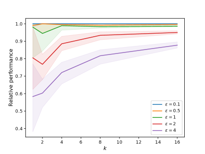
(b) Discogs

Figure 1: Relative performance of the greedy method on sparsifiers.

In this section, we empirically demonstrate that our algorithm (Algorithm 2) generates a sparse representation of a decomposable submodular function $F:2^{E}\to\mathbb{R}_{+}$ with which we can efficiently obtain a high-quality solution for maximizing $F$. We consider the following two settings.

Uber pickup. We used a database of Uber pickups in New York city in May 2014 consisting of a set $R$ of 564,517 records. Each record has a pickup position, longitude and latitude. Consider selecting $k$ locations as waiting spots for idle Uber drivers. To formalize this problem, we selected a set $L$ of 36 popular pickup locations in the database, and constructed a facility location function $F:2^{L}\to\mathbb{R}_{+}$ as $F(S)=\sum_{v\in R}f_{v}(S)$, where $f_{v}(S)=\max_{u\in L}d(u,v)-\min_{u\in S}d(u,v)$ and $d(u,v)$ is the Manhattan distance between $u$ and $v$. Then, the goal of the problem is to maximize $F(S)$ subject to $|S|\leq k$.

Discogs Kunegis (2013). This dataset provides information about audio records as a bipartite graph $G=(L,R;E)$, where each edge $(u,v)\in L\times R$ indicates that a label $v$ was involved in the production of a release of a style $u$. We have $|L|=383$ and $|R|=243,764$, and $|E|=5,255,950$. Consider selecting $k$ styles that cover the activity of as many labels as possible. To formalize this problem, we constructed a maximum coverage function $F:2^{L}\to\mathbb{R}$ as $F(S)=\sum_{v\in R}f_{v}(S)$, where $f_{v}(S)$ is $1$ if $v$ has a neighbor in $S$ and $0$ otherwise. Then, the goal is to maximize $F(S)$ subject to $|S|\leq k$.

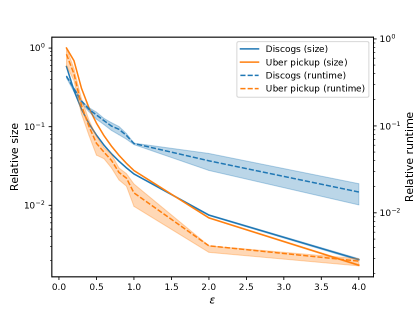
Figure 2: Relative size of sparsifiers and relative runtime of the greedy method on sparsifiers.

Figure 1 shows the objective value of the solution obtained by the greedy method on the sparsifier relative to that on the original input function with its 25th and 75th percentiles. Although our theoretical results do not give any guarantee when $\epsilon>1$, we tried constructing our sparsifier with $\epsilon>1$ to see its performance. The solution quality of our sparsifier for Uber pickup is more than 99.9% even when $\epsilon=4$, and that for Discogs is more than 90% performance when $\epsilon\leq 1.0$. The performance for Uber pickup is higher than that for Discogs because the objective function of the former saturates easily. These results suggest that we get a reasonably good solution quality by setting $\epsilon=1$.

Number of functions and speedups.

Figure 2 shows the size, that is, the number of functions with positive weights, of our sparsifier relative to that of the original function and the runtime of the greedy method on the sparsifier relative to that on the original function with their 25th and 75th percentiles when $k=8$. The size and runtime are decreased by a factor of 30–50 when $\epsilon=1$. To summarize, our experimental results suggest that our sparsifier highly compresses the original function without sacrificing the solution quality.

Conclusion

Decomposable submodular functions appear in many data intensive tasks in machine learning and data mining. Thus, having a sparsifying algorithm is of great interest. In this paper, we introduce the notion of sparsifier for decomposable submodular functions. We propose the first sparsifying algorithm for these types of functions which outputs accurate sparsifiers with expected size independent of the size of original function. Our algorithm can be adapted to sparsify mixtures of submodular functions. We also study the effectiveness of our algorithm under various constraints such as matroid and cardinality constraints. Our experimental results complement our theoretical results on real world data. This work does not present any foreseeable societal consequence.

7 Missing proofs

7.1 Proof of Claim 3.3

Proof.

$$\sum\limits_{i\in D}p_{i} =\sum\limits_{i\in D}\max\limits_{A\subseteq E}\frac{f_{i}(A)}{F(A)}=\sum\limits_{i\in D}\max\limits_{A\subseteq E}\frac{f_{i}(A)}{\sum\limits_{j\in D}f_{j}(A)}$$

$$=\sum\limits_{i\in D}\max\limits_{A\subseteq E}\frac{\max\limits_{{\bm{y}}\in\mathcal{B}(f_{i})}\langle{{\bm{y}},{\bm{1}}_{A}\rangle}}{\sum\limits_{j\in D}\max\limits_{{\bm{y}}\in\mathcal{B}(f_{j})}\langle{{\bm{y}},{\bm{1}}_{A}\rangle}}$$

$$\leq\sum\limits_{i\in D}\max\limits_{A\subseteq E}\frac{\sum\limits_{{\bm{y}}\in\mathcal{B}(f_{i})}\langle{{\bm{y}},{\bm{1}}_{A}\rangle}}{\sum\limits_{j\in D}\frac{1}{|\mathcal{B}(f_{j})|}\sum\limits_{{\bm{y}}\in\mathcal{B}(f_{j})}\langle{{\bm{y}},{\bm{1}}_{A}\rangle}}$$

$$\leq\sum\limits_{i\in D}\max\limits_{A\subseteq E}\max\limits_{e\in A}\frac{\sum\limits_{{\bm{y}}\in\mathcal{B}(f_{i})}{\bm{y}}(e)}{\sum\limits_{j\in D}\frac{1}{|\mathcal{B}(f_{j})|}\sum\limits_{{\bm{y}}\in\mathcal{B}(f_{j})}{\bm{y}}(e)}$$

$$=\sum\limits_{i\in D}\max\limits_{e\in E}\frac{\sum\limits_{{\bm{y}}\in\mathcal{B}(f_{i})}{\bm{y}}(e)}{\sum\limits_{j\in D}\frac{1}{|\mathcal{B}(f_{j})|}\sum\limits_{{\bm{y}}\in\mathcal{B}(f_{j})}{\bm{y}}(e)}$$

$$\leq\sum\limits_{i\in D}\sum\limits_{e\in E}\frac{\sum\limits_{{\bm{y}}\in\mathcal{B}(f_{i})}{\bm{y}}(e)}{\sum\limits_{j\in D}\frac{1}{|\mathcal{B}(f_{j})|}\sum\limits_{{\bm{y}}\in\mathcal{B}(f_{j})}{\bm{y}}(e)}$$

$$=\sum\limits_{e\in E}\sum\limits_{i\in D}\frac{\sum\limits_{{\bm{y}}\in\mathcal{B}(f_{i})}{\bm{y}}(e)}{\sum\limits_{j\in D}\frac{1}{|\mathcal{B}(f_{j})|}\sum\limits_{{\bm{y}}\in\mathcal{B}(f_{j})}{\bm{y}}(e)}$$

$$\leq\sum\limits_{e\in E}\max\limits_{j\in D}|\mathcal{B}(f_{j})|\sum\limits_{i\in D}\frac{\sum\limits_{{\bm{y}}\in\mathcal{B}(f_{i})}{\bm{y}}(e)}{\sum\limits_{j\in D}\sum\limits_{{\bm{y}}\in\mathcal{B}(f_{j})}{\bm{y}}(e)}$$

$$\leq\sum\limits_{e\in E}\max\limits_{j\in D}|\mathcal{B}(f_{j})|\frac{\sum\limits_{i\in D}\sum\limits_{{\bm{y}}\in\mathcal{B}(f_{i})}{\bm{y}}(e)}{\sum\limits_{j\in D}\sum\limits_{{\bm{y}}\in\mathcal{B}(f_{j})}{\bm{y}}(e)}$$

$$=\sum\limits_{e\in E}\max\limits_{j\in D}|\mathcal{B}(f_{j})|=n\cdot(\max_{j\in D}|\mathcal{B}(f_{j})|).$$

∎

7.2 Proof of Theorem 4.1

Proof.

The proof is almost identical to the proof of Lemma 3.1. We prove that for every $S\in\mathcal{I}$ with high probability it holds that $(1-\epsilon)F^{\prime}(S)\leq F^{L}(S)\leq(1+\epsilon)F^{\prime}(S)$. Observe that by our choice of $p_{i}$ and ${\bm{w}}_{i}$ we have $\mathbb{E}[F^{\prime}(S)]=F(S)$, for all subsets $S\in\mathcal{M}$. Consider a subset $S_{k}$. Using Theorem 2.2, we have

$$\mathbb{P}\left[|F^{\prime}(S_{k})-\mathbb{E}[F^{\prime}(S_{k})]|\geq\epsilon\mathbb{E}[F^{\prime}(S_{k})]\right]$$ (12)

$$=\mathbb{P}\left[|F^{\prime}(S_{k})-F(S_{k})|\geq\epsilon F(S_{k})\right]$$ (13)

$$\leq 2\exp{\left(\nicefrac{{-\epsilon^{2}F(S_{k})}}{{3a}}\right)}$$ (14)

where $a=\max_{i}{\bm{w}}_{i}f_{i}(S_{k})$. We bound the right hand side of (14) by providing an upper bound for $a$.

$$a =\max\limits_{i}{\bm{w}}_{i}f_{i}(S_{k})=\max\limits_{i}\frac{f_{i}(S_{k})}{\kappa\cdot p_{i}}$$

$$=\max\limits_{i}\frac{f_{i}(S_{k})}{\kappa\cdot\max\limits_{A\in\mathcal{I}}\frac{f_{i}(A)}{F(A)}}$$

$$\leq\max\limits_{i}\frac{f_{i}(S_{k})}{\kappa\cdot\frac{f_{i}(S_{k})}{F(S_{k})}}=\frac{F(S_{k})}{\kappa}.$$

Given the above upper bound for $a$ and the inequality in (14) yields

$$\mathbb{P}\left[|F^{\prime}(S_{k})-F(S_{k})|\geq\epsilon F(S_{k})\right]\leq 2\exp{\left(-\frac{\epsilon^{2}F(S_{k})}{3a}\right)}$$

$$\leq 2\exp{\left(-\frac{\epsilon^{2}F(S_{k})}{3F(S_{k})/\kappa}\right)}=2\exp{\left(\nicefrac{{-\kappa\epsilon^{2}}}{{3}}\right)}$$

Recall that $\kappa=3\log(2n^{r+1}/\delta)/\epsilon^{2}$. Note that there are at most $n^{r}$ sets in a matroid of rank $r$. Taking a union bound over all $n^{r}$ subsets yields that Algorithm 2 with probability at least $1-\delta$ returns a sparsifier for $F$ over the matroid. Similar to Lemma 3.2, $\sum_{i\in D}p_{i}\leq n\cdot(\max_{i\in D}|B(f_{i})|)$, and having $\kappa=3\log(2n^{r+1}/\delta)/\epsilon^{2}$ gives

$$\mathbb{E}[\mathrm{size}({\bm{w}})]\leq\sum_{i}\kappa p_{i}\leq O\left(\frac{rn}{\epsilon^{2}}\cdot\max\limits_{i\in D}|B(f_{i})|\right).$$

∎

7.3 Proof of Theorem 4.2

Proof.

The proof is almost the same as that of Theorem 3.5 (Theorem 3.5 in Bai et al. (2016)). Therefore, we only explain modifications we need to handle a matroid constraint.

In the algorithm used in Theorem 3.5, given a monotone modular function $f:2^{E}\to\mathbb{R}_{+}$, a monotone submodular function $g:2^{E}\to\mathbb{R}_{+}$, and a threshold $c\in\mathbb{R}_{+}$, we iteratively solve the following problem:

$$\begin{array}[]{ll}\text{minimize}&f(X),\\ \text{subject to}&g(X)\geq c.\end{array}$$ (17)

We say that an algorithm for solving (17) a $(\sigma,\rho)$-bicriterion algorithm if it outputs $X\subseteq E$ such that $f(X)\leq\sigma f(X^{*})$ and $g(X)\geq\rho c$, where $X^{*}$ is the optimal solution. It is shown in Bai et al. (2016) that a $(\sigma,\rho)$-bicriterion algorithm for constant $\sigma$ and $\rho$ leads to an $O(\sqrt{n}\log n)$-approximation algorithm for maximizing $g(X)/f(X)$.

If we have an additional matroid constraint $\mathcal{M}=(E,\mathcal{I})$, we need a bicriterion algorithm for the following problem:

$$\begin{array}[]{ll}\text{minimize }&f(X),\\ \text{subject to}&g(X)\geq c,\\ &X\in\mathcal{I}.\end{array}$$ (21)

To solve (21), we consider the following problem.

$$\begin{array}[]{ll}\text{maximize }&g(X),\\ \text{subject to}&f(X)\leq d,\\ &X\in\mathcal{I}.\end{array}$$ (25)

This problem is a monotone submodular function maximization problem subject to an intersection of a matroid constraint and a knapsack constraint (recall that $f$ is modular), and is known to admit $\alpha$-approximation for some constant $\alpha$ Vondrák et al. (2011). Then by computing an $\alpha$-approximate solution $X$ for every $d$ of the form $2^{i}$, and take the minimum $d$ such that $g(X)\geq\alpha\cdot c$, we obtain a $(1,\alpha)$-bicriterion approximation to (21), as desired. ∎

7.4 Proof of Theorem 5.2

Proof.

It follows from the fact that $F^{L}({\bm{x}})$ is a linear combination of $F(S)$, $S\subseteq E$. More precisely, for a decomposable submodular function $F=\sum_{i\in D}f_{i}$, its Lovász extension is

$$F^{L}({\bm{x}}) =\sum\limits_{j=0}^{n}\sum\limits_{i\in D}({\bm{x}}_{\pi(j)}-{\bm{x}}_{\pi(j+1)})f_{i}(S_{j}^{\pi})$$ (26)

$$=\sum\limits_{j=0}^{n}({\bm{x}}_{\pi(j)}-{\bm{x}}_{\pi(j+1)})\sum\limits_{i\in D}f_{i}(S_{j}^{\pi})$$ (27)

$$=\sum\limits_{j=0}^{n}({\bm{x}}_{\pi(j)}-{\bm{x}}_{\pi(j+1)})F(S_{j}^{\pi})$$ (28)

Now since our sparsifier approximates $F(S)$ for all subsets $S\subseteq E$ we have

$$(1-\epsilon)F^{\prime}(S_{j}^{\pi})\leq F(S_{j}^{\pi})\leq(1+\epsilon)F^{\prime}(S_{j}^{\pi})\quad 0\leq j\leq n$$ (29)

Finally, (28) and (29) yield the following

$$(1-\epsilon)F^{\prime L}({\bm{w}})\leq F^{L}({\bm{x}})\leq(1+\epsilon)F^{\prime L}({\bm{x}})\quad\forall{\bm{x}}\in[0,1]^{n}.$$

∎

References

- Ahn et al. [2012] Kook Jin Ahn, Sudipto Guha, and Andrew McGregor. Graph sketches: sparsification, spanners, and subgraphs. In PODS, pages 5–14, 2012. doi: 10.1145/2213556.2213560. URL https://doi.org/10.1145/2213556.2213560.
- Ahn et al. [2013] Kook Jin Ahn, Sudipto Guha, and Andrew McGregor. Spectral sparsification in dynamic graph streams. In APPROX, pages 1–10, 2013. doi: 10.1007/978-3-642-40328-6“˙1. URL https://doi.org/10.1007/978-3-642-40328-6_1.
- Andoni et al. [2016] Alexandr Andoni, Jiecao Chen, Robert Krauthgamer, Bo Qin, David P. Woodruff, and Qin Zhang. On sketching quadratic forms. In ITCS, pages 311–319, 2016. doi: 10.1145/2840728.2840753. URL https://doi.org/10.1145/2840728.2840753.
- Axiotis et al. [2021] Kyriakos Axiotis, Adam Karczmarz, Anish Mukherjee, Piotr Sankowski, and Adrian Vladu. Decomposable submodular function minimization via maximum flow. In ICML, pages 446–456, 2021. URL http://proceedings.mlr.press/v139/axiotis21a.html.
- Bai et al. [2016] Wenruo Bai, Rishabh K. Iyer, Kai Wei, and Jeff A. Bilmes. Algorithms for optimizing the ratio of submodular functions. In ICML, pages 2751–2759, 2016. URL http://proceedings.mlr.press/v48/baib16.html.
- Bairi et al. [2015] Ramakrishna Bairi, Rishabh K. Iyer, Ganesh Ramakrishnan, and Jeff A. Bilmes. Summarization of multi-document topic hierarchies using submodular mixtures. In ACL, pages 553–563, 2015. doi: 10.3115/v1/p15-1054. URL https://doi.org/10.3115/v1/p15-1054.
- Bansal et al. [2019] Nikhil Bansal, Ola Svensson, and Luca Trevisan. New notions and constructions of sparsification for graphs and hypergraphs. In FOCS, pages 910–928, 2019. doi: 10.1109/FOCS.2019.00059. URL https://doi.org/10.1109/FOCS.2019.00059.
- Batson et al. [2012] Joshua D. Batson, Daniel A. Spielman, and Nikhil Srivastava. Twice-Ramanujan sparsifiers. SIAM J. Comput., 41(6):1704–1721, 2012. doi: 10.1137/090772873. URL https://doi.org/10.1137/090772873.
- Benczúr and Karger [1996] András A. Benczúr and David R. Karger. Approximating s-t minimum cuts in Õ(n) time. In STOC, pages 47–55, 1996. doi: 10.1145/237814.237827. URL https://doi.org/10.1145/237814.237827.
- Benczúr and Karger [2015] András A. Benczúr and David R. Karger. Randomized approximation schemes for cuts and flows in capacitated graphs. SIAM J. Comput., 44(2):290–319, 2015. doi: 10.1137/070705970. URL https://doi.org/10.1137/070705970.
- Chaturvedi et al. [2021] Anamay Chaturvedi, Huy Le Nguyen, and Lydia Zakynthinou. Differentially private decomposable submodular maximization. In AAAI, pages 6984–6992, 2021. URL https://ojs.aaai.org/index.php/AAAI/article/view/16860.
- Chen et al. [2020] Yu Chen, Sanjeev Khanna, and Ansh Nagda. Near-linear size hypergraph cut sparsifiers. In FOCS, pages 61–72, 2020. doi: 10.1109/FOCS46700.2020.00015. URL https://doi.org/10.1109/FOCS46700.2020.00015.
- Cohen et al. [2015] Michael B. Cohen, Yin Tat Lee, Cameron Musco, Christopher Musco, Richard Peng, and Aaron Sidford. Uniform sampling for matrix approximation. In ITCS, pages 181–190, 2015. doi: 10.1145/2688073.2688113. URL https://doi.org/10.1145/2688073.2688113.
- Cohen et al. [2017] Michael B. Cohen, Jonathan Kelner, John Peebles, Richard Peng, Anup B. Rao, Aaron Sidford, and Adrian Vladu. Almost-linear-time algorithms for markov chains and new spectral primitives for directed graphs. In STOC, pages 410–419, 2017. doi: 10.1145/3055399.3055463. URL https://doi.org/10.1145/3055399.3055463.
- Dobzinski and Schapira [2006] Shahar Dobzinski and Michael Schapira. An improved approximation algorithm for combinatorial auctions with submodular bidders. In SODA, pages 1064–1073, 2006. URL http://dl.acm.org/citation.cfm?id=1109557.1109675.
- Dueck and Frey [2007] Delbert Dueck and Brendan J. Frey. Non-metric affinity propagation for unsupervised image categorization. In ICCV, pages 1–8, 2007. doi: 10.1109/ICCV.2007.4408853. URL https://doi.org/10.1109/ICCV.2007.4408853.
- Edmonds [2001] Jack Edmonds. Submodular functions, matroids, and certain polyhedra. In Combinatorial Optimization - Eureka, You Shrink!, pages 11–26, 2001.
- Ene et al. [2017] Alina Ene, Huy L. Nguyen, and László A. Végh. Decomposable submodular function minimization: Discrete and continuous. In NeurIPS, pages 2870–2880, 2017. URL https://proceedings.neurips.cc/paper/2017/hash/c1fea270c48e8079d8ddf7d06d26ab52-Abstract.html.
- Feige [2006] Uriel Feige. On maximizing welfare when utility functions are subadditive. In STOC, pages 41–50, 2006. doi: 10.1145/1132516.1132523. URL https://doi.org/10.1145/1132516.1132523.
- Feige and Vondrák [2006] Uriel Feige and Jan Vondrák. Approximation algorithms for allocation problems: Improving the factor of 1 - 1/e. In FOCS, pages 667–676, 2006. doi: 10.1109/FOCS.2006.14. URL https://doi.org/10.1109/FOCS.2006.14.
- Fix et al. [2013] Alexander Fix, Thorsten Joachims, Sung Min Park, and Ramin Zabih. Structured learning of sum-of-submodular higher order energy functions. In ICCV, pages 3104–3111, 2013. doi: 10.1109/ICCV.2013.385. URL https://doi.org/10.1109/ICCV.2013.385.
- Gomes and Krause [2010] Ryan Gomes and Andreas Krause. Budgeted nonparametric learning from data streams. In ICML, pages 391–398, 2010. URL https://icml.cc/Conferences/2010/papers/433.pdf.
- Kapralov et al. [2021a] Michael Kapralov, Robert Krauthgamer, Jakab Tardos, and Yuichi Yoshida. Towards tight bounds for spectral sparsification of hypergraphs. In STOC, pages 598–611, 2021a. doi: 10.1145/3406325.3451061. URL https://doi.org/10.1145/3406325.3451061.
- Kapralov et al. [2021b] Michael Kapralov, Robert Krauthgamer, Jakab Tardos, and Yuichi Yoshida. Spectral hypergraph sparsifiers of nearly linear size. In FOCS, 2021b.
- Karger and Levine [2002] David R. Karger and Matthew S. Levine. Random sampling in residual graphs. In STOC, pages 63–66, 2002. doi: 10.1145/509907.509918. URL https://doi.org/10.1145/509907.509918.
- Kogan and Krauthgamer [2015] Dmitry Kogan and Robert Krauthgamer. Sketching cuts in graphs and hypergraphs. In ITCS, pages 367–376, 2015. doi: 10.1145/2688073.2688093. URL https://doi.org/10.1145/2688073.2688093.
- Kohli et al. [2009] Pushmeet Kohli, Lubor Ladicky, and Philip H. S. Torr. Robust higher order potentials for enforcing label consistency. Int. J. Comput. Vis., 82(3):302–324, 2009. doi: 10.1007/s11263-008-0202-0. URL https://doi.org/10.1007/s11263-008-0202-0.
- Kunegis [2013] J. Kunegis. Konect: the koblenz network collection. In WWW, Companion Volume, pages 1343–1350, 2013. doi: 10.1145/2487788.2488173. URL https://doi.org/10.1145/2487788.2488173.
- Lee and Sidford [2014] Yin Tat Lee and Aaron Sidford. Path finding methods for linear programming: Solving linear programs in õ(vrank) iterations and faster algorithms for maximum flow. In FOCS, pages 424–433, 2014. doi: 10.1109/FOCS.2014.52. URL https://doi.org/10.1109/FOCS.2014.52.
- Lee and Sun [2018] Yin Tat Lee and He Sun. Constructing linear-sized spectral sparsification in almost-linear time. SIAM J. Comput., 47(6):2315–2336, 2018. doi: 10.1137/16M1061850. URL https://doi.org/10.1137/16M1061850.
- Li et al. [2013] Mu Li, Gary L. Miller, and Richard Peng. Iterative row sampling. In FOCS, pages 127–136, 2013. doi: 10.1109/FOCS.2013.22. URL https://doi.org/10.1109/FOCS.2013.22.
- Li and Milenkovic [2017] Pan Li and Olgica Milenkovic. Inhomogeneous hypergraph clustering with applications. In NeurIPS, pages 2308–2318, 2017. URL https://proceedings.neurips.cc/paper/2017/hash/a50abba8132a77191791390c3eb19fe7-Abstract.html.
- Li and Milenkovic [2018] Pan Li and Olgica Milenkovic. Submodular hypergraphs: p-laplacians, cheeger inequalities and spectral clustering. In ICML, pages 3020–3029, 2018. URL http://proceedings.mlr.press/v80/li18e.html.
- Lin and Bilmes [2011] Hui Lin and Jeff A. Bilmes. A class of submodular functions for document summarization. In HLT, pages 510–520, 2011.
- Lindgren et al. [2016] Erik M. Lindgren, Shanshan Wu, and Alexandros G. Dimakis. Leveraging sparsity for efficient submodular data summarization. In NeurIPS, pages 3414–3422, 2016. URL https://proceedings.neurips.cc/paper/2016/hash/d43ab110ab2489d6b9b2caa394bf920f-Abstract.html.
- Madry [2010] Aleksander Madry. Fast approximation algorithms for cut-based problems in undirected graphs. In FOCS, pages 245–254, 2010. doi: 10.1109/FOCS.2010.30. URL https://doi.org/10.1109/FOCS.2010.30.
- Mahoney [2011] Michael W. Mahoney. Randomized algorithms for matrices and data. Found. Trends Mach. Learn., 3(2):123–224, 2011. doi: 10.1561/2200000035. URL https://doi.org/10.1561/2200000035.
- Mirzasoleiman et al. [2015] Baharan Mirzasoleiman, Ashwinkumar Badanidiyuru, Amin Karbasi, Jan Vondrák, and Andreas Krause. Lazier than lazy greedy. In AAAI, pages 1812–1818, 2015. URL http://www.aaai.org/ocs/index.php/AAAI/AAAI15/paper/view/9956.
- Mirzasoleiman et al. [2016a] Baharan Mirzasoleiman, Ashwinkumar Badanidiyuru, and Amin Karbasi. Fast constrained submodular maximization: Personalized data summarization. In ICML, pages 1358–1367, 2016a. URL http://proceedings.mlr.press/v48/mirzasoleiman16.html.
- Mirzasoleiman et al. [2016b] Baharan Mirzasoleiman, Amin Karbasi, Rik Sarkar, and Andreas Krause. Distributed submodular maximization. J. Mach. Learn. Res., 17:238:1–238:44, 2016b. URL http://jmlr.org/papers/v17/mirzasoleiman16a.html.
- Mirzasoleiman et al. [2016c] Baharan Mirzasoleiman, Morteza Zadimoghaddam, and Amin Karbasi. Fast distributed submodular cover: Public-private data summarization. In NeurIPS, pages 3594–3602, 2016c. URL http://papers.nips.cc/paper/6540-fast-distributed-submodular-cover-public-private-data-summarization.
- Mitrovic et al. [2017] Marko Mitrovic, Mark Bun, Andreas Krause, and Amin Karbasi. Differentially private submodular maximization: Data summarization in disguise. In ICML, pages 2478–2487, 2017. URL http://proceedings.mlr.press/v70/mitrovic17a.html.
- Mitrovic et al. [2018] Marko Mitrovic, Ehsan Kazemi, Morteza Zadimoghaddam, and Amin Karbasi. Data summarization at scale: A two-stage submodular approach. In ICML, volume 80, pages 3593–3602, 2018. URL http://proceedings.mlr.press/v80/mitrovic18a.html.
- Motwani and Raghavan [1995] Rajeev Motwani and Prabhakar Raghavan. Randomized Algorithms. Cambridge University Press, 1995. ISBN 0-521-47465-5. doi: 10.1017/cbo9780511814075. URL https://doi.org/10.1017/cbo9780511814075.
- Nemhauser et al. [1978] George L. Nemhauser, Laurence A. Wolsey, and Marshall L. Fisher. An analysis of approximations for maximizing submodular set functions - I. Math. Program., 14(1):265–294, 1978. doi: 10.1007/BF01588971. URL https://doi.org/10.1007/BF01588971.
- Papadimitriou et al. [2008] Christos H. Papadimitriou, Michael Schapira, and Yaron Singer. On the hardness of being truthful. In FOCS, pages 250–259, 2008. doi: 10.1109/FOCS.2008.54. URL https://doi.org/10.1109/FOCS.2008.54.
- Parambath et al. [2016] Shameem Puthiya Parambath, Nicolas Usunier, and Yves Grandvalet. A coverage-based approach to recommendation diversity on similarity graph. In RecSys, pages 15–22, 2016. doi: 10.1145/2959100.2959149. URL https://doi.org/10.1145/2959100.2959149.
- Rafiey and Yoshida [2020] Akbar Rafiey and Yuichi Yoshida. Fast and private submodular and k-submodular functions maximization with matroid constraints. In ICML, pages 7887–7897, 2020. URL http://proceedings.mlr.press/v119/rafiey20a.html.
- Shanu et al. [2016] Ishant Shanu, Chetan Arora, and Parag Singla. Min norm point algorithm for higher order MRF-MAP inference. In CVPR, pages 5365–5374, 2016. doi: 10.1109/CVPR.2016.579. URL https://doi.org/10.1109/CVPR.2016.579.
- Soma and Yoshida [2019] Tasuku Soma and Yuichi Yoshida. Spectral sparsification of hypergraphs. In SODA, pages 2570–2581, 2019. doi: 10.1137/1.9781611975482.159. URL https://doi.org/10.1137/1.9781611975482.159.
- Spielman and Teng [2011] Daniel A. Spielman and Shang-Hua Teng. Spectral sparsification of graphs. SIAM J. Comput., 40(4):981–1025, 2011. doi: 10.1137/08074489X. URL https://doi.org/10.1137/08074489X.
- Stobbe and Krause [2010] Peter Stobbe and Andreas Krause. Efficient minimization of decomposable submodular functions. In NeurIPS, pages 2208–2216, 2010. URL https://proceedings.neurips.cc/paper/2010/hash/6ea2ef7311b482724a9b7b0bc0dd85c6-Abstract.html.
- Tschiatschek et al. [2014] Sebastian Tschiatschek, Rishabh K. Iyer, Haochen Wei, and Jeff A. Bilmes. Learning mixtures of submodular functions for image collection summarization. In NeurIPS, pages 1413–1421, 2014. URL https://proceedings.neurips.cc/paper/2014/hash/a8e864d04c95572d1aece099af852d0a-Abstract.html.
- Veldt et al. [2020a] Nate Veldt, Austin R. Benson, and Jon M. Kleinberg. Minimizing localized ratio cut objectives in hypergraphs. In KDD, pages 1708–1718, 2020a. doi: 10.1145/3394486.3403222. URL https://doi.org/10.1145/3394486.3403222.
- Veldt et al. [2020b] Nate Veldt, Austin R. Benson, and Jon M. Kleinberg. Hypergraph cuts with general splitting functions. CoRR, abs/2001.02817, 2020b. URL http://arxiv.org/abs/2001.02817.
- Vicente et al. [2009] Sara Vicente, Vladimir Kolmogorov, and Carsten Rother. Joint optimization of segmentation and appearance models. In ICCV, pages 755–762, 2009. doi: 10.1109/ICCV.2009.5459287. URL https://doi.org/10.1109/ICCV.2009.5459287.
- Vondrák [2008] Jan Vondrák. Optimal approximation for the submodular welfare problem in the value oracle model. In STOC, pages 67–74, 2008. doi: 10.1145/1374376.1374389. URL https://doi.org/10.1145/1374376.1374389.
- Vondrák et al. [2011] Jan Vondrák, Chandra Chekuri, and Rico Zenklusen. Submodular function maximization via the multilinear relaxation and contention resolution schemes. In STOC, pages 783–792, 2011. doi: 10.1145/1993636.1993740. URL https://doi.org/10.1145/1993636.1993740.
- Yoshida [2016] Yuichi Yoshida. Nonlinear Laplacian for digraphs and its applications to network analysis. In WSDM, pages 483–492, 2016. doi: 10.1145/2835776.2835785. URL https://doi.org/10.1145/2835776.2835785.
- Yoshida [2019] Yuichi Yoshida. Cheeger inequalities for submodular transformations. In SODA, pages 2582–2601, 2019. doi: 10.1137/1.9781611975482.160. URL https://doi.org/10.1137/1.9781611975482.160.