Constraints on Single-Field Inflation from the BOSS Galaxy Survey

Abstract

Non-local primordial non-Gaussianity (NLPNG) is a smoking gun of interactions in single-field inflationary models, and can be written as a combination of the equilateral and orthogonal templates. We present the first constraints on these from the redshift-space galaxy power spectra and bispectra of the Baryon Oscillation Spectroscopic Survey (BOSS) data. These are the first such measurements independent of the cosmic microwave background fluctuations. We perform a consistent analysis that includes all necessary nonlinear corrections generated by NLPNG, and vary all relevant cosmological and nuisance parameters in a global fit to the data. Our conservative analysis yields joint limits on the amplitudes of the equilateral and orthogonal shapes, $f_{\rm NL}^{\rm equil}=940\pm 600$, $f_{\rm NL}^{\rm ortho}=-170\pm 170$ (both at 68% CL). These can be used to derive constraints on coefficients of the effective single-field inflationary Lagrangian; in particular, we find that the sound speed of inflaton fluctuations has the bound $c_{s}\geq 0.013$ at 95% CL. Fixing the quadratic galaxy bias and cosmological parameters, the constraints can be tightened to $f_{\rm NL}^{\rm equil}=260\pm 300$, $f_{\rm NL}^{\rm ortho}=-23\pm 120$ (68% CL).

Introduction — Cosmology is the interface between particle physics and general relativity. Nothing exemplifies this more than inflation – a primordial accelerated expansion of the Universe that may have happened at energy scales as high as $10^{14}\,{\rm GeV}$. Inflation naturally generates quantum fluctuations that provide the seeds for the formation and clustering of matter and galaxies. Thus, observations of the large-scale structure of our Universe allow us to probe physics at these extremely high energies, inaccessible to present-day particle accelerators.

There are three main questions about inflation one may ask: What is its energy scale? How many degrees of freedom generated density fluctuations? How fast did these degrees of freedom propagate? While significant efforts have been devoted to answering the first question, by constraining the amplitude of primordial gravitational waves, the latter two require a probe of deviations of the initial density fluctuations from a Gaussian distribution, known as primordial non-Gaussianity (PNG).

The simplest observable encoding PNG is the bispectrum, $B_{\zeta}$, of the primordial metric curvature perturbation $\zeta$. Due to translational and rotational invariance, $B_{\zeta}$ is a function of the moduli of three momenta, ${\bf k}_{1},{\bf k}_{2},{\bf k}_{3}$, which form a closed triangle. A bispectrum peaking at squeezed triangles, $k_{1}\ll k_{2}\approx k_{3}$, is a generic signature of particle interactions in multi-field inflation Linde and Mukhanov (1997); Enqvist and Sloth (2002); Lyth and Wands (2002); Lyth et al. (2003); Dvali et al. (2004a, b); Zaldarriaga (2004); Byrnes and Choi (2010); Senatore and Zaldarriaga (2012), i.e. where more than one degree of freedom is light during inflation. This type of PNG is called “local”. In contrast, a bispectrum peaking at equilateral ($k_{1}\approx k_{2}\approx k_{3}$) or flattened ($k_{1}\approx k_{2}\approx k_{3}/2$) triangles is a peculiar feature of interactions in single-field inflation Arkani-Hamed et al. (2004); Alishahiha et al. (2004); Senatore (2005); Chen et al. (2007); Creminelli et al. (2006); Cheung et al. (2008a, b); Senatore et al. (2010), which has only one degree of freedom (inflaton). This kind of “non-local” primordial non-Gaussianity (NLPNG) can be represented as a linear combination of two basis shapes, equilateral and orthogonal Senatore et al. (2010), with amplitudes $f_{\rm NL}^{\rm equil}$ and $f_{\rm NL}^{\rm ortho}$ respectively.

Symmetries of inflation also dictate a relationship between the inflaton speed of sound and the strength of nonlinear interactions that generate NLPNG Cheung et al. (2008a). In particular, there is a theorem stating that PNG can be large if and only if the sound speed is small Baumann et al. (2016); Green and Pajer (2020). This allows one to constrain the propagation speed of the inflaton from the observed level of NLPNG.

Up to now, the only source of information on NLPNG has been the cosmic microwave background (CMB) temperature and polarization data Bennett et al. (2013); Akrami et al. (2020). In particular, Planck 2018 data yield $f_{\rm NL}^{\rm equil}=-26\pm 47$, $f_{\rm NL}^{\rm ortho}=-38\pm 24$ (both at 68% CL) Akrami et al. (2020). In theory, one can obtain better constraints with upcoming galaxy surveys, which will collect orders of magnitude more cosmological information as counted in number of accessible Fourier modes. However, the analysis of this data is also more intricate because PNG in the galaxy distribution is a weak effect on top of an intrinsic, late-time non-Gaussian signal generated by nonlinear clustering of matter. Thus, late-time nonlinearities act as background noise, which must be accurately modeled if we are to measure PNG from large-scale structure data.

There have been significant efforts to probe local PNG from galaxy surveys, exploiting the scale-dependent bias that enhances the observed power spectrum on very large scales Leistedt et al. (2014); Castorina et al. (2019); Mueller et al. (2021). This enhancement originates from a particular form of the squeezed limit of the local shape. NLPNG is different as the relevant shapes are suppressed in the squeezed limit and hence do not produce significant scale-dependent bias. Thus, this type of PNG requires a dedicated study. Indeed, the leading effect of NLPNG on galaxy clustering is a specific shape dependence in the galaxy bispectrum, which also modulates power spectra through loop corrections. These effects can be constrained by a systematic analysis based on the consistently-modeled power spectrum and bispectrum data. In this Letter, we present the first such analysis of the publicly available state of the art redshift clustering data from the Baryon Oscillation Spectroscopic Survey (BOSS).

A rigorous analysis of the galaxy bispectrum has been a long-time challenge. Even ignoring PNG, the complete theoretical model including all necessary effects relevant for the actual data has been developed only recently Ivanov et al. (2021a); Philcox and Ivanov (2021) (see also Scoccimarro (2000); Sefusatti et al. (2006); Baldauf et al. (2015a); Angulo et al. (2015a); Eggemeier et al. (2018); Ivanov et al. (2020a); D’Amico et al. (2019); Oddo et al. (2020); Eggemeier et al. (2021); Alkhanishvili et al. (2021); Oddo et al. (2021); Chen et al. (2021); Baldauf et al. (2021)). On the data side, a major improvement has come from the estimators that remove effects of the survey window function Philcox (2021a, b). These efforts now allow us to obtain the first CMB-independent limits on NLPNG from galaxy redshift surveys.

PNG in single-field inflation — A general single-field Lagrangian for the inflaton perturbation $\pi$ with leading interactions up to cubic order is given by Cheung et al. (2008a); Senatore et al. (2010)

$$\begin{split}&S_{\rm EFT}=\int{\rm d}^{4}x\sqrt{-g}\Bigg{[}{-\frac{M_{\rm P}^{2}\dot{H}}{c_{s}^{2}}}\left(\dot{\pi}^{2}-c_{s}^{2}\frac{({\bm{\nabla}}\pi)^{2}}{a^{2}}\right)\\ &+\frac{M_{\rm P}^{2}\dot{H}}{c_{s}^{2}}(1-c_{s}^{2})\left(\frac{\dot{\pi}({\bm{\nabla}}\pi)^{2}}{a^{2}}-\left(1+\frac{2}{3}\frac{\tilde{c}_{3}}{c_{s}^{2}}\right)\dot{\pi}^{3}\right)\Bigg{]}\,\,.\end{split}$$ (1)

$\pi$ is related to the metric curvature perturbation via $\zeta=-H\pi$, with $H$ being the Hubble parameter during inflation. The two inflaton interactions are parametrized by the sound speed $c_{s}$ and a dimensionless Wilson coefficient $\tilde{c}_{3}$. It is customary to represent PNG produced by these interactions as a linear combination of the orthogonal and equilateral templates. To that end, we define

$$B_{\zeta}(k_{1},k_{2},k_{3})=\frac{18}{5}f_{\rm NL}\Delta^{4}_{\zeta}\frac{{\cal S}(k_{1},k_{2},k_{3})}{k_{1}^{2}k_{2}^{2}k_{3}^{2}}\,\,.$$ (2)

Here, $\Delta^{2}_{\zeta}$ is the amplitude of the primordial power spectrum: $k^{3}P_{\zeta}(k)=\Delta^{2}_{\zeta}(k/k_{\ast})^{n_{s}-1}$, where $n_{s}$ is the spectral index. Analysis of Planck data finds $\Delta^{2}_{\zeta}\approx 4.1\times 10^{-8}$, $n_{s}\approx 0.96$ Aghanim et al. (2018) for the pivot scale $k_{\ast}=0.05$ Mpc^-1. The equilateral and orthogonal templates are defined as Babich et al. (2004); Senatore et al. (2010)

$$\begin{split}&{\cal S}_{\rm equil}(k_{1},k_{2},k_{3})=\\ &\bigg{(}\frac{k_{1}}{k_{2}}+\text{$5$ perms.}\bigg{)}-\bigg{(}\frac{k_{1}^{2}}{k_{2}k_{3}}+\text{$2$ perms.}\bigg{)}-2\,\,,\\ &{\cal S}_{\rm ortho}(k_{1},k_{2},k_{3})=(1+p)\,\frac{\Delta}{e_{3}}-p\,\frac{\Gamma^{3}}{e_{3}^{2}}\,\,,\end{split}$$ (3)

where $p=8.52587$, $\Delta=(k_{T}-2k_{1})(k_{T}-2k_{2})(k_{T}-2k_{3})$,

$$\begin{split}&k_{T}=k_{1}+k_{2}+k_{3}\,\,,\quad e_{2}=k_{1}k_{2}+k_{2}k_{3}+k_{1}k_{3}\,\,,\\ &e_{3}=k_{1}k_{2}k_{3}\,\,,\quad\Gamma=\frac{2}{3}e_{2}-\frac{1}{3}(k_{1}^{2}+k_{2}^{2}+k_{3}^{2})\,\,.\end{split}$$ (4)

The amplitudes $f_{\rm NL}^{\rm equil}$, $f_{\rm NL}^{\rm ortho}$ are related to the cofficients of the EFT Lagrangian via Babich et al. (2004); Senatore et al. (2010)

$$\begin{split}\begin{pmatrix}f_{\rm NL}^{\rm equil}\\ f_{\rm NL}^{\rm ortho}\end{pmatrix}&=\begin{pmatrix}1.04021&1.21041\\ -0.0395140&-0.175685\end{pmatrix}\begin{pmatrix}f_{\rm NL}^{\dot{\pi}({\bm{\nabla}}\pi)^{2}}\\ f_{\rm NL}^{\dot{\pi}^{3}}\end{pmatrix}\,\,,\\ f_{\rm NL}^{\dot{\pi}({\bm{\nabla}}\pi)^{2}}&=\frac{85}{324}(1-c_{s}^{-2})\,,\\ f_{\rm NL}^{\dot{\pi}^{3}}&=\frac{10}{243}(1-c_{s}^{-2})\left(\tilde{c}_{3}+\frac{3}{2}c_{s}^{2}\right)\,.\end{split}$$ (5)

Large Scale Structure in the presence of NLPNG — Before considering NLPNG, we first discuss structure formation in a Universe with Gaussian initial conditions. We describe it in the framework of the effective field theory of large-scale structure (EFTofLSS), where one builds a perturbative expansion in terms of the linear matter overdensity field $\delta^{(1)}$  (see Baumann et al. (2012); Carrasco et al. (2012); Desjacques et al. (2018); Ivanov et al. (2020a); D’Amico et al. (2019); Nishimichi et al. (2020) and references therein). For Gaussian initial conditions, statistical properties of $\delta^{(1)}$ are fully determined by its power spectrum $P_{11}$

$$\langle\delta^{(1)}({\bf k})\delta^{(1)}({\bf k}^{\prime})\rangle=(2\pi)^{3}\delta^{(3)}_{D}({\bf k}^{\prime}+{\bf k})P_{11}(k)\,\,.$$ (6)

We restrict our galaxy power spectrum analysis to the one-loop order in the EFTofLSS. In the absence of NLPNG, the nonlinear power spectrum takes the following schematic form

$$P_{\rm G}\equiv P_{11}+P_{\rm 1-loop}+P_{\rm ctr}+P_{\rm stoch}\,\,,$$ (7)

where $P_{\rm 1-loop}$ is the nonlinear one-loop correction for Gaussian initial conditions, $P_{\rm ctr}$ is the counterterm that stems from the higher-derivative operators in the fluid equation and the bias expansion, while $P_{\rm stoch}$ captures galaxy stochasticity. Nonlinear clustering also generates a non-trivial “Gaussian” bispectrum $B_{\rm G}$, which we consider here in the tree-level approximation.

PNG affects large-scale structure via three channels: initial conditions, loop corrections, and scale-dependent galaxy bias. First, PNG induces a bispectrum signal additional to the one coming from nonlinear mode coupling Sefusatti and Komatsu (2007); Sefusatti (2009),

$$\begin{split}&\langle\delta^{(1)}\delta^{(1)}\delta^{(1)}\rangle=f_{\rm NL}B_{111}(k_{1},k_{2},k_{3})(2\pi)^{3}\delta^{(3)}_{D}({\bf k}_{123})\,\,,\\ &f_{\rm NL}B_{111}(k_{1},k_{2},k_{3})=\mathcal{T}(k_{1})\mathcal{T}(k_{2})\mathcal{T}(k_{3})B_{\zeta}(k_{1},k_{2},k_{3})\,\,,\end{split}$$ (8)

where ${\bf k}_{123}={\bf k}_{1}+{\bf k}_{2}+{\bf k}_{3}$, and we introduced the transfer functions $\mathcal{T}(k)\equiv\delta^{(1)}({\bf k})/\zeta({\bf k})=(P_{11}(k)/P_{\zeta}(k))^{1/2}$. The initial bispectrum (8) also leaks into the nonlinear galaxy power spectra through mode coupling, and induces the following non-Gaussian one-loop correction (which adds to $P_{\rm G}$ above)

$$\begin{split}&f_{\rm NL}P_{12}(\textbf{k})=2f_{\rm NL}Z_{1}({\bf k})\\ &\times\int\frac{{\rm d}^{3}q}{(2\pi)^{3}}Z_{2}({\bf q},{\bf k}-{\bf q})B_{111}(k,q,|{\bf k}-{\bf q}|)\,\,.\end{split}$$ (9)

Here $Z_{1,2}$ are linear and quadratic galaxy redshift-space kernels Chudaykin et al. (2020), $Z_{1}({\bf k})=b_{1}+f(\hat{{\bf k}}\cdot\hat{\mathbf{z}})^{2}$ where $f$ is the logarithmic growth factor, $\hat{\mathbf{z}}$ is the line-of-sight direction unit vector, and $\hat{{\bf k}}\equiv{\bf k}/k$. The $P_{12}$ terms are present for both galaxies and matter Taruya et al. (2008); Assassi et al. (2015a); Moradinezhad Dizgah et al. (2021), and we will refer to them as “NG matter loops” in what follows.

Third, NLPNG modulates galaxy formation, which is captured on large scales by the scale-dependent galaxy bias Assassi et al. (2015b); Angulo et al. (2015b); Desjacques et al. (2018),

$$\delta_{g}=b_{1}\delta+f_{\rm NL}b_{\zeta}(k/k_{\rm NL})^{2}\zeta+\text{nonlinear}\,\,,$$ (10)

where $\delta$ and $\delta_{g}$ are overdensity fields of matter and galaxies respectively, $b_{1}$ is the usual linear bias, $b_{\zeta}$ is an order-one PNG linear bias coefficient, and $k_{\rm NL}\approx 0.5\,h\text{Mpc}^{-1}$ is the nonlinear scale at the relevant redshift $z\simeq 0.5$.

The relative size of various perturbative corrections can be estimated using the scaling universe approach Pajer and Zaldarriaga (2013); Assassi et al. (2015a). It is based on the observation that the linear power spectrum can be well approximated by a power-law $P_{11}\propto(k/k_{\rm NL})^{n}k_{\rm NL}^{-3}$ with $n\approx-1.7$ for quasi-linear wavenumbers $k\simeq 0.15\,h\text{Mpc}^{-1}$. Assuming that there is a single nonlinear scale in the problem, the scaling universe estimates suggest that the leading non-Gaussian corrections are the PNG matter loops and the linear scale-dependent bias. The total dimensionless galaxy power spectrum $\Delta^{2}(k)\equiv k^{3}P(k)/(2\pi^{2})$ can be estimated as

$$\begin{split}\Delta^{2}(k)&={\underbrace{\left(\frac{k}{k_{\rm NL}}\right)^{1.3}}_{\rm tree}}+\underbrace{\left(\frac{k}{k_{\rm NL}}\right)^{2.6}}_{\rm 1-loop}+\underbrace{\left(\frac{k}{k_{\rm NL}}\right)^{3.3}}_{\rm ctr}+\underbrace{\left(\frac{k}{k_{\rm NL}}\right)^{3}}_{\rm stoch}\\ &+\underbrace{f_{\rm NL}\Delta_{\zeta}\left(\frac{k}{k_{\rm NL}}\right)^{1.95}}_{\text{NG matter loops}}+\underbrace{f_{\rm NL}b_{\zeta}\Delta_{\zeta}\left(\frac{k}{k_{\rm NL}}\right)^{2.65}}_{\text{linear PNG bias}}\,\,.\end{split}$$ (11)

All higher order corrections, such as PNG terms $\mathcal{O}(f_{\rm NL}^{2})$, NG two-loop corrections, contributions generated by nonlinear bias operators like $\delta\nabla^{2}\zeta$, and Gaussian two-loop corrections, are subleading for $f_{\rm NL}\Delta_{\zeta}\lesssim 0.1$ and $k\lesssim 0.17~{}h\text{Mpc}^{-1}$ typical for our analysis, and hence can be neglected. This will be validated on the mock simulation data below. As for the bispectrum, we use the tree-level approximation so only the leading PNG bispectrum (8) is of importance Assassi et al. (2015a).

All in all, our final model for the galaxy power spectra and bispectra in redshift space is given by

$$\begin{split}&P({\bf k})=P_{\rm G}({\bf k})+f_{\rm NL}\left(P_{12}({\bf k})+\frac{2b_{\zeta}Z_{1}({\bf k})k^{2}}{k_{\rm NL}^{2}}\frac{P_{11}(k)}{\mathcal{T}(k)}\right)\,,\\ &B({\bf k}_{1},{\bf k}_{2},{\bf k}_{3})=B_{\rm G}({\bf k}_{1},{\bf k}_{2},{\bf k}_{3})\\ &~{}~{}~{}~{}+f_{\rm NL}Z_{1}({\bf k}_{1})Z_{1}({\bf k}_{2})Z_{1}({\bf k}_{3})B_{111}(k_{1},k_{2},k_{3})\,\,,\end{split}$$ (12)

where $P_{\rm G}$ and $B_{\rm G}$ are the standard Gaussian power spectrum and bispectrum models Ivanov et al. (2020b, 2021a). In practice, we compute the Legendre redshift-space multipoles $P_{\ell}$ ($\ell=0,2,4$) of the galaxy power spectrum and use the angle-averaged (monopole) bispectrum. We also implement IR resummation in redshift space Senatore and Zaldarriaga (2015); Baldauf et al. (2015b); Blas et al. (2016a, b); Ivanov and Sibiryakov (2018); Vasudevan et al. (2019) (to account for long-wavelength displacement effects) and the Alcock-Paczynski effect Alcock and Paczynski (1979) (to account for coordinate conversions Ivanov et al. (2020a)).

Our model has 14 nuisance parameters: 13 standard bias parameters and counterterms of Gaussian redshift-space power spectra and bispectra (present in previous analyses), plus the scale-dependent PNG bias $b_{\zeta}$ (10). ,

Data and Analysis — We use the twelfth data release (DR12) Alam et al. (2017) of BOSS. The data is split into two redshift bins with effective means $z=0.38,0.61$, in each of the Northern and Southern galactic caps, resulting in four independent data chunks. The survey contains $\sim 1.2\times 10^{6}$ galaxy positions with a total volume of $6\,(h^{-1}\text{Gpc})^{3}$. From each chunk, we use the power spectrum multipoles ($\ell=0,2,4$) for $k\in[0.01,0.17)\,h\text{Mpc}^{-1}$, the real-space power spectrum $Q_{0}$ for $k\in[0.17,0.4)\,h\text{Mpc}^{-1}$ Ivanov et al. (2021b), the redshift-space bispectrum monopoles for triangle configurations within the range of $k_{i}\in[0.01,0.08)\,h\text{Mpc}^{-1}$ (62 triangles), and the BAO parameters extracted from the post-reconstructed power spectrum data Philcox et al. (2020), as in Philcox and Ivanov (2021). The power spectra and bispectra are measured with the window-free estimators Philcox (2021a, b). The covariances for each data chunk are computed from a suite of 2048 MultiDark-Patchy mocks Kitaura et al. (2016).

Figure 1: Marginalized constraints on parameters ($f_{\rm NL}^{\rm equil},f_{\rm NL}^{\rm ortho}$) from the BOSS data obtained in the conservative baseline analysis (BOSS DR12 (B), gray), and in the aggressive analysis (BOSS DR12 (A), blue). We also show results from the full Nseries simulation suite (red), whose volume is 40 times larger than BOSS. Dashed lines indicate $f_{\rm NL}^{\rm equil}=0,f_{\rm NL}^{\rm ortho}=0$.

Figure 2: Marginalized constraints on single-field inflation parameters ($c_{s},\tilde{c}_{3}$) from the BOSS data in the baseline analysis (BOSS DR12 (B), gray), aggressive analysis (BOSS DR12 (A), blue), and from the full Nseries simulation suite (red).

We perform the full-shape analysis of the redshift clustering data following the methodology of Ivanov et al. (2020a); D’Amico et al. (2019); Philcox et al. (2020); Philcox and Ivanov (2021). We implement the complete theory model for the power spectra and bispectra of galaxies in redshift space in an extension of the CLASS-PT code Chudaykin et al. (2020) that includes all non-Gaussian corrections described above (computed using the FFTlog approach Simonović et al. (2018)). We consistently recompute the shape of these corrections as we scan over different cosmologies in a Markov Chain Monte Carlo (MCMC) analysis. Up to additional NG contributions, our analysis is identical to Philcox and Ivanov (2021).

In our baseline analysis we fix the baryon density to the BBN measurement Cooke et al. (2018), the primordial power spectrum tilt to the Planck best-fit value Aghanim et al. (2018), and the neutrino mass to the minimal value allowed by oscillation experiments $\sum m_{\nu}=0.06$ eV. We vary the physical dark matter density $\omega_{cdm}$, the reduced Hubble parameter $h$, the amplitude of the primordial scalar fluctuations $\mathop{\rm ln}\nolimits(10^{10}A_{s})$, and $(f_{\rm NL}^{\rm equil},f_{\rm NL}^{\rm ortho})$ within flat infinitely wide priors. We use the same priors for nuisance parameters as Philcox and Ivanov (2021). We also marginalize over the linear PNG bias, $b_{\zeta}=1.686\cdot\frac{18}{5}(b_{1}-1)\tilde{b}_{\zeta}$ within a Gaussian prior $\tilde{b}_{\zeta}\sim\mathcal{N}(1,5)$ motivated by the peak-background split model Schmidt and Kamionkowski (2010).

In addition, we perform a more aggressive analysis, whereupon cosmological parameters are set to the Planck 2018 priors. Moreover, instead of marginalization, we fix the quadratic galaxy biases to predictions of the standard dark matter halo relations Desjacques et al. (2018). These agree with simulations at the level required by the BOSS data Eggemeier et al. (2021); Ivanov et al. (2021a).

It is worth noting that our analysis is different from the CMB one Senatore et al. (2010), where $f_{\rm NL}$ is estimated directly from the temperature and polarization maps. In contrast, we do a global fit to the summary statistics, and vary $f_{\rm NL}^{\rm equil},f_{\rm NL}^{\rm ortho}$ along with all other cosmological and nuisance parameters in our MCMC chains, necessary due to the appearance of parameter-dependent late-time non-Gaussianity.

Results — First, we apply our pipeline to Nseries mock catalogs. These are based on high-resolution N-body simulations and were used by the BOSS collaboration for validation tests Alam et al. (2017). The cumulative volume of this simulation is $235\,(h^{-1}\text{Gpc})^{3}$, which is $\approx 40$ times larger than actual BOSS survey volume. The mocks were generated from purely Gaussian initial conditions, which we must recover with our pipeline as a consistency check. Indeed, we find $f_{\rm NL}^{\rm equil}=240_{-130}^{+130}$, $f_{\rm NL}^{\rm ortho}=-6_{-54}^{+52}$, which is consistent with $f_{\rm NL}^{\rm equil}=0$ within 95% CL and $f_{\rm NL}^{\rm ortho}=0$ within 68% CL. The shift in $f_{\rm NL}^{\rm equil}$, even if statistically insignificant, yields an estimate of the theoretical uncertainty, $\Delta f_{\rm NL}^{\rm equil}\lesssim 100$, which is less than $0.2\sigma$ of the BOSS 1d marginalized statistical error. This is consistent with estimates of higher order perturbative corrections that are omitted in our analysis. We have also found that the constraints are driven by the bispectrum: the power spectrum data alone gives $f_{\rm NL}^{\rm equil}=-640\pm 1200$, $f_{\rm NL}^{\rm ortho}=2400\pm 1600$ (at 68% CL).

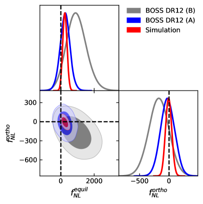
Having validated our method on the simulations, we move to the actual BOSS data. Our baseline MCMC analysis yields the following 1d marginalized estimates of equilateral and orthogonal $f_{\rm NL}$ values from the joint fit:

$$f_{\rm NL}^{\rm equil}=940_{-650}^{+570}\,\,,\quad f_{\rm NL}^{\rm ortho}=-170_{-170}^{+180}\,\,,\quad\text{(68\%~{}CL)}\,\,.$$ (13)

We do not find any evidence for NLPNG: the 95% CL limits read

$$-280<f_{\rm NL}^{\rm equil}<2190\,\,,\quad-520<f_{\rm NL}^{\rm ortho}<176\,\,.$$ (14)

The resulting posterior contours are shown in Fig. 1. The correlation coefficient between the equilateral and orthogonal shapes is $-0.40$. The best measured principal component is

$$f_{\rm NL}^{\rm ortho}-0.11f_{\rm NL}^{\rm equil}=-65\pm 157\,\,.$$

Note that the correlation is dictated by degeneracy directions in the shape of the BOSS galaxy bispectrum. This can be contrasted with the Planck 2018 data that does not show any appreciable degeneracy between the two shapes, i.e. their correlation matches the intrinsic template cosine Akrami et al. (2020). This implies that combinations with the CMB data will be important for degeneracy breaking in future analyses.

Our aggressive analysis yields noticeably stronger constraints, $f_{\rm NL}^{\rm equil}=257_{-300}^{+300}$, $f_{\rm NL}^{\rm ortho}=-23_{-120}^{+120}$. Most of the improvement here is driven by fixing quadratic bias parameters. In light of the well-known $\sigma_{8}$ tension, we have also varied $\sigma_{8}$ in our aggressive fit, which somewhat loosens the bounds, $f_{\rm NL}^{\rm equil}=510_{-440}^{+320}$, $f_{\rm NL}^{\rm ortho}=-123_{-140}^{+150}$ ($\sigma_{8}=0.728_{-0.037}^{+0.033}$), at 68% CL. Concluding, we emphasize that our aggressive analysis is performed mainly for the purposes of illustration. It demonstrates that PNG constraints can be significantly improved with a better knowledge of bias parameters, which motivates further work on their calibration with simulations, e.g. along the lines of Barreira et al. (2021); Lazeyras et al. (2021).

We have also repeated our baseline analysis with free $n_{s}$ and found consistent, albeit somewhat weaker limits $f_{\rm NL}^{\rm equil}=1200_{-850}^{+630}$, $f_{\rm NL}^{\rm ortho}=-240_{-180}^{+210}$ (with $n_{s}=0.83\pm 0.08$).

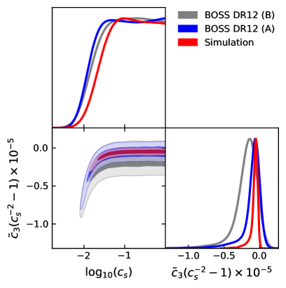
Constraints on early Universe physics — Our main analysis was performed using flat priors on $f_{\rm NL}^{\rm equil},f_{\rm NL}^{\rm ortho}$, which map onto non-flat priors of the physical coefficients in the EFT Lagrangian (1). To avoid any potential prior bias, we repeat our MCMC analysis varying directly the relevant parameters $\log_{10}c_{s}$ and $\tilde{c}_{3}(c_{s}^{-2}-1)$ (following Senatore et al. (2010)), assuming flat priors $\log_{10}c_{s}\in(-\infty,0]$ and $\tilde{c}_{3}(c_{s}^{-2}-1)\in(-\infty,+\infty)$. The corresponding posterior contours are shown in Fig. 2. They yield the bound on the sound speed

$$c_{s}\geq 0.013\quad(\tilde{c}_{3}~{}\text{marginalized, 95\%~{}CL})\,\,.$$ (15)

For DBI inflation Alishahiha et al. (2004), where $\tilde{c}_{3}=3(1-c_{s}^{2})/2$, we find $c_{s}\geq 0.04$ (95% CL). In general, the parameter $\tilde{c}_{3}$ cannot be constrained because of degeneracy with $c_{s}$, i.e. $\tilde{c}_{3}$ is unbounded in the limit $c_{s}\to 1$, where we can only constrain the combination of the two parameters,

$${-3.5}\times 10^{4}<\tilde{c}_{3}(c_{s}^{-2}-1)<1\times 10^{4}\quad\text{(95\%~{}CL)}\,\,.$$ (16)

Constraints on $c_{s}$ do not noticeably improve with the aggressive analysis settings. This is because the $(f_{\rm NL}^{\rm equil},f_{\rm NL}^{\rm ortho})$ parameter space excluded by these settings mostly corresponds to the unphysical values $c_{s}^{2}>1$, $c_{s}^{2}<0$, and hence does not contribute to our final constraints on this parameter.

Conclusions — In this Letter we have presented the first non-CMB constraints on non-local primordial non-Gaussianity, using the BOSS redshift-space clustering data. Our nominal constraints on the orthogonal shape and the inflaton sound speed are competitive with those from the Wilkinson Microwave Anisotropy Probe CMB data Bennett et al. (2013). These constraints will certainly improve with the data from upcoming surveys such as Euclid Laureijs et al. (2011) or DESI Aghamousa et al. (2016). Based on their volume w.r.t. BOSS, one may expect a reduction of error bars by a factor of $3$. However, the limits from current and future surveys can be improved even further if more bispectrum data is used, e.g. from new triangles with larger wavenumbers, and from the angular dependence captured by higher order harmonics (multipoles) of the redshift-space bispectrum Scoccimarro (2015). We leave including this information for future work. In addition, it would be interesting to analyze more complex PNG scenarios, and also include information from the recently measured BOSS galaxy trispectrum Philcox et al. (2021).

Finally, it is worth noting that the PNG constraints from large-scale structure will further improve with futuristic surveys, such as MegaMapper Schlegel et al. (2019), and 21cm/intensity mapping observations, which will map our Universe at high redshifts where the late-time non-Gaussian clustering background is weak.

Our work thus serves as a proof of principle, and paves the way toward systematic analyses of PNG with upcoming large-scale structure surveys.

Acknowledgments — We are grateful to Alex Barreira, Enrico Pajer, and Fabian Schmidt for valuable comments on the draft. GC acknowledges support from the Institute for Advanced Study. The work of MMI has been supported by NASA through the NASA Hubble Fellowship grant #HST-HF2-51483.001-A awarded by the Space Telescope Science Institute, which is operated by the Association of Universities for Research in Astronomy, Incorporated, under NASA contract NAS5-26555. OHEP thanks the Simons Foundation for support. Parameter estimates presented in this paper have been obtained with the CLASS-PT Boltzmann code Chudaykin et al. (2020) (see also Blas et al. (2011)) interfaced with the Montepython MCMC sampler Audren et al. (2013); Brinckmann and Lesgourgues (2019). The triangle plots are generated with the getdist package Lewis (2019).

Supplemental Material

1 Details of the theory model

Following the notation of Chudaykin et al. (2020), the $Z_{2}$ kernel necessary to derive $P_{12}(\mathbf{k})$ in Eq. (9) is

$$\begin{split}Z_{2}({\bf k}_{1},{\bf k}_{2})&=\frac{b_{2}}{2}+b_{\mathcal{G}_{2}}\bigg{(}\frac{({\bf k}_{1}\cdot{\bf k}_{2})^{2}}{k_{1}^{2}k_{2}^{2}}-1\bigg{)}+b_{1}F_{2}({\bf k}_{1},{\bf k}_{2})+f\mu^{2}G_{2}({\bf k}_{1},{\bf k}_{2})\\ &\;\;\;\;+\frac{f\mu k}{2}\bigg{(}\frac{\mu_{1}}{k_{1}}(b_{1}+f\mu_{2}^{2})+\frac{\mu_{2}}{k_{2}}(b_{1}+f\mu_{1}^{2})\bigg{)}\,\,,\end{split}$$ (S1)

where $F_{2}$ and $G_{2}$ are the SPT kernels Bernardeau et al. (2002)

$$\begin{split}F_{2}({\bf k}_{1},{\bf k}_{2})&=\frac{5}{7}+\frac{2}{7}\frac{({\bf k}_{1}\cdot{\bf k}_{2})^{2}}{k_{1}^{2}k_{2}^{2}}+\frac{1}{2}\frac{{\bf k}_{1}\cdot{\bf k}_{2}}{k_{1}k_{2}}\bigg{(}\frac{k_{1}}{k_{2}}+\frac{k_{2}}{k_{1}}\bigg{)}\,\,,\\ G_{2}({\bf k}_{1},{\bf k}_{2})&=\frac{3}{7}+\frac{4}{7}\frac{({\bf k}_{1}\cdot{\bf k}_{2})^{2}}{k_{1}^{2}k_{2}^{2}}+\frac{1}{2}\frac{{\bf k}_{1}\cdot{\bf k}_{2}}{k_{1}k_{2}}\bigg{(}\frac{k_{1}}{k_{2}}+\frac{k_{2}}{k_{1}}\bigg{)}\,\,,\end{split}$$ (S2)

and $\mu_{i}=\hat{\mathbf{k}}_{i}\cdot\hat{\mathbf{z}}$. Our non-Gaussian model depends on the quadratic bias $b_{2}$ and the tidal bias $b_{\mathcal{G}_{2}}$, which also enter the tree-level bispectrum model. For dark matter halos, these biases have the following approximate dependence on the linear bias $b_{1}$:

$$b_{\mathcal{G}_{2}}=-\frac{2}{7}(b_{1}-1)\,\,,\quad b_{2}=0.412-2.143b_{1}+0.929b_{1}^{2}+0.008b_{1}^{2}-\frac{8}{21}(b_{1}-1)\,\,.$$ (S3)

The relationship $b_{\mathcal{G}_{2}}(b_{1})$ follows from the Lagrangian local in matter density model Desjacques et al. (2018), while the function $b_{2}(b_{1})$ is fit from the halo simulation data Lazeyras et al. (2016). These relationships, strictly speaking, do not hold for simulated galaxies, but the deviations are not significant given the precision of the current data Eggemeier et al. (2021); Ivanov et al. (2021a). We use the relations (S3) in our aggressive analysis, evaluating them for the best-fit values of $b_{1}$ taken from the baseline results.

2 Effects of PNG on galaxy power spectra and bispectra

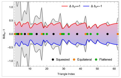
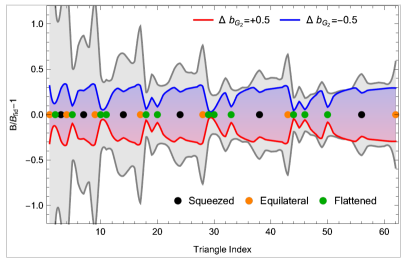
In this Section we present plots that give some intuition on the source of our $f_{\rm NL}$ constraints. In Fig. S1 we illustrate the effect of variations of the parameters $f_{\rm NL}^{\rm equil},f_{\rm NL}^{\rm ortho},b_{2},b_{\mathcal{G}_{2}}$ on the galaxy bispectrum monopole $B$. Parameters are varied within the following intervals:

$$f_{\rm NL}^{\rm equil}\in[-2000,2000]\,\,,\quad f_{\rm NL}^{\rm ortho}\in[-1000,1000]\,\,,\quad b_{2}\in[b_{2}^{\rm fid}-1,b_{2}^{\rm fid}+1]\,\,,\quad b_{\mathcal{G}_{2}}\in[b_{\mathcal{G}_{2}}^{\rm fid}-0.5,b_{\mathcal{G}_{2}}^{\rm fid}+0.5]\,\,,$$ (S4)

where $b_{2}^{\rm fid},b^{\rm fid}_{\mathcal{G}_{2}}$ are fiducial parameters equal to the best-fit values. We present the residuals $B/B_{\rm fid.}-1$ as a function of the triangle index of our bispectrum data vector, where $B_{\rm fid.}$ is the best-fit bispectrum model for the NGC z3 ($z=0.61$) data chunk, obtained in the analysis with $f_{\rm NL}^{\rm equil}=0,f_{\rm NL}^{\rm ortho}=0$. Each triangle is labelled by its bin center wavenumbers ($k_{1},k_{2},k_{3}$), whose magnitudes are constrained to be $k\in[0.015,0.08)~{}h\text{Mpc}^{-1}$. Indices corresponding to squeezed, equilateral, and flattened configurations are denoted by black, orange, and green dots in the $x$ axis, and a shaded gray contour on the background shows the error bars of the NGC z3 data. We chose the extremal values of the varied parameters in Eq. (S4) such that the resulting residual curve has a $1\sigma$ deviation at least for several data points. This suggests that the cumulative $\chi^{2}$ should be significant, and the corresponding variations should be constrained by the data.

Figure S1: Residual variations of the galaxy bispectrum monopole w.r.t. variations of $f_{\rm NL}^{\rm equil}$ (upper left panel), $f_{\rm NL}^{\rm ortho}$ (upper right panel), quadratic bias $b_{2}$ (lower left panel), and tidal bias $b_{\mathcal{G}_{2}}$ (lower right panel). Black, orange and green dots denote the squeezed ($k_{3}=0.015~{}h\text{Mpc}^{-1}$, $k_{2}=k_{1}$), equilateral ($k_{1}=k_{2}=k_{3}$), and flattened ($k_{2}=k_{3}$, $2k_{2}=k_{1}+0.005~{}h\text{Mpc}^{-1}$) triangle configurations, respectively. These variations have distinctive shape dependence and therefore can be constrained by the data.

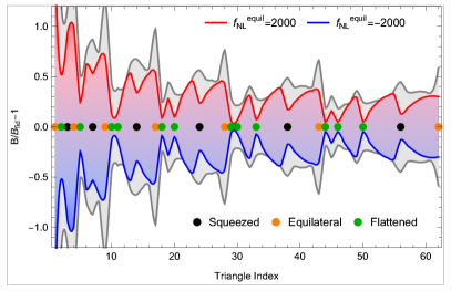
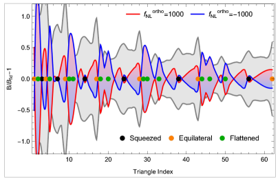
The first important observation is that the parameters of interest have very different shape dependence. $f_{\rm NL}^{\rm equil}$ mostly enhances equilateral triangles ($k_{1}=k_{2}=k_{3}$); the effect on the squeezed triangles ($k_{3}=0.015\,h\text{Mpc}^{-1}$, $k_{1}=k_{2}$, $k_{1}>k_{3}$) is somewhat weaker, whilst the flattened triangles ($k_{3}=k_{2}$, $2k_{2}=k_{1}+0.005\,h\text{Mpc}^{-1}$) are affected very little. In contrast, $f_{\rm NL}^{\rm ortho}$ peaks sharply at the flattened and equilateral triangles. Note that these effects are of the opposite sign, which is a known signature of the orthogonal template. Remarkably, the effect on the squeezed triangles is vanishingly small.

Now let us discuss the quadratic bias parameters, which represent a late-time non-Gaussian contribution. The effect of $b_{2}$ is almost uniform for all triangles. In contrast, $b_{\mathcal{G}_{2}}$ noticeably amplifies the squeezed and equilateral triangles, while the flattened triangles are almost unaffected.

All in all, we see that the data should distinguish between the shapes of interest. The qualitative picture of that is as follows. $f_{\rm NL}^{\rm ortho}$ is the only shape that sharply peaks at the flattened triangles. In addition, it produces specific “opposite” peaks in the equilateral triangles. Clearly, this pattern cannot be reproduced by any other parameter and hence we do not expect $f_{\rm NL}^{\rm ortho}$ to be degenerate with them. The signature of $b_{2}$ is also quite unique, as it is the only shape that enhances all triangles in a uniform way. Hence, it should be robustly constrained. The only noticeable degeneracy we expect is between $f_{\rm NL}^{\rm equil}$ and $b_{\mathcal{G}_{2}}$, because both corresponding shapes mostly enhance squeezed and equilateral configurations, while leaving the flattened triangles almost intact. The degeneracy between these gets broken by the relative height of the squeezed and equilateral triangles: $b_{\mathcal{G}_{2}}$ enhances both these triangles uniformly, while $f_{\rm NL}^{\rm equil}$ generates some contrast by amplifying more the equilateral configurations.

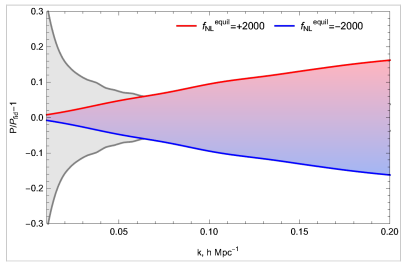
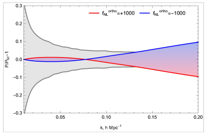
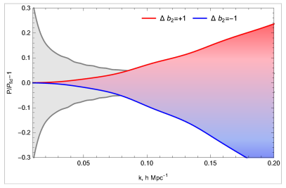
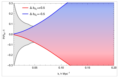
In Fig. S2 we repeat the same exercise for the galaxy power spectrum monopole $P$ for the wavenumbers relevant for our analysis, $k\in[0.01,0.2)\,h\text{Mpc}^{-1}$. We focus on the $P_{12}$-type matter loop corrections only, because the effects of the linear PNG bias clearly cannot be constrained without a prior on $b_{\zeta}$. Looking at Fig. S2, we see that, although power spectrum modulations produced by $f_{\rm NL}^{\rm equil}\sim 1000$, $f_{\rm NL}^{\rm ortho}\sim 1000$ are nominally larger than the error bars, the signal produced by these shapes is a very smooth function of scale. Thus, the PNG terms are quite degenerate with the Gaussian non-linear corrections, explaining why we cannot get strong constraints on NLPNG from the power spectra alone. For very large $f_{\rm NL}^{\rm equil},f_{\rm NL}^{\rm ortho}$, however, one can break the degeneracies, i.e. using the non-monotonic behaviour of the $f_{\rm NL}^{\rm ortho}$ term on large scales $\lesssim 0.1\,h\text{Mpc}^{-1}$. This explains why in the mock simulation data analysis we were able to break degeneracies for very large $f_{\rm NL}^{\rm ortho}\sim 1000$. However, the total volume of this simulation was $40$ times larger than the actual BOSS survey volume. This demonstrates that the galaxy power spectrum alone does not have enough power to provide any interesting constraints on PNG, though it is still instrumental in breaking parameter degeneracies relevant for the bispectrum, e.g. the notorious degeneracy between $b_{1}$ and $\sigma_{8}$.

Figure S2: Residual variations of the galaxy power spectrum monopole $P_{0}$ w.r.t. variations of $f_{\rm NL}^{\rm equil}$ (upper left panel), $f_{\rm NL}^{\rm ortho}$ (upper right panel), quadratic bias $b_{2}$ (lower left panel), and tidal bias $b_{\mathcal{G}_{2}}$ (lower right panel).

3 Full triangle plots and constraint tables

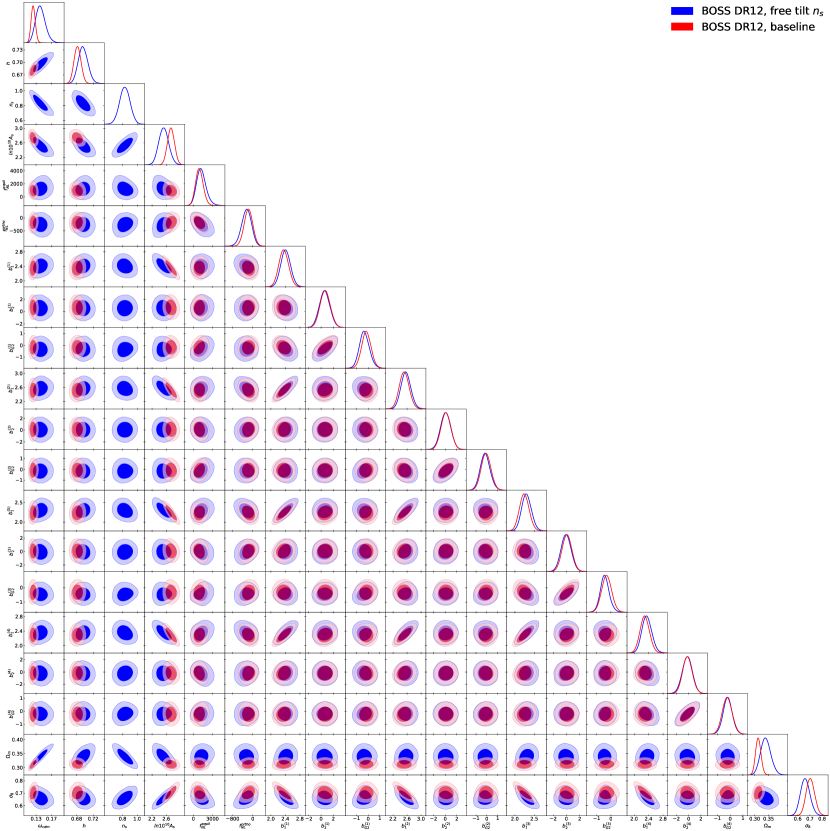
In this Section we present a full triangle plot (Fig. S3) and parameter constraint table (Tab. 1) from two PNG analyses of BOSS DR12: (a) with free power spectrum tilt $n_{s}$ and (b) with a Planck prior on $n_{s}$. The latter is our baseline choice. We present results for the joint analysis of the full power spectrum, BAO, and bispectrum datasets.

	BOSS DR12 + free $n_{s}$				BOSS DR12, baseline
Parameter	best-fit	mean$\,\pm\,\sigma$	95% lower	95% upper	best-fit	mean$\,\pm\,\sigma$	95% lower	95% upper
$\omega_{cdm}$	$0.1262$	$0.1413_{-0.015}^{+0.011}$	$0.1159$	$0.1682$	$0.1197$	$0.1225_{-0.0059}^{+0.0053}$	$0.1115$	$0.1339$
$h$	$0.6848$	$0.6954_{-0.013}^{+0.011}$	$0.6719$	$0.7195$	$0.6827$	$0.682_{-0.0088}^{+0.0085}$	$0.665$	$0.6992$
$\mathrm{ln}\left(10^{10}A_{s}\right)$	$2.739$	$2.533_{-0.15}^{+0.14}$	$2.249$	$2.826$	$2.716$	$2.728_{-0.1}^{+0.1}$	$2.528$	$2.929$
$n_{s}$	$0.9324$	$0.8323_{-0.074}^{+0.075}$	$0.6858$	$0.9801$	-	-	-	-
$10^{-2}f^{\rm equil}_{{\rm NL}}$	$1.82$	$12.39_{-8.6}^{+6.7}$	$-3.179$	$28.49$	$2.278$	$9.421_{-6.5}^{+5.7}$	$-2.779$	$21.91$
$10^{-2}f^{\rm ortho}_{{\rm NL}}$	$-0.0628$	$-2.484_{-1.9}^{+2.1}$	$-6.557$	$1.484$	$-0.7874$	$-1.732_{-1.7}^{+1.8}$	$-5.265$	$1.756$
$b^{(1)}_{1}$	$2.323$	$2.404_{-0.14}^{+0.14}$	$2.127$	$2.687$	$2.408$	$2.353_{-0.14}^{+0.13}$	$2.078$	$2.63$
$b^{(1)}_{2}$	$0.5561$	$0.5731_{-0.9}^{+0.84}$	$-1.159$	$2.295$	$0.9517$	$0.675_{-0.88}^{+0.83}$	$-1.012$	$2.396$
$b^{(1)}_{{\mathcal{G}_{2}}}$	$-0.3561$	$-0.324_{-0.46}^{+0.41}$	$-1.197$	$0.57$	$-0.1242$	$-0.1568_{-0.42}^{+0.41}$	$-0.9911$	$0.6793$
$b^{(2)}_{1}$	$2.502$	$2.566_{-0.15}^{+0.14}$	$2.282$	$2.858$	$2.563$	$2.521_{-0.15}^{+0.14}$	$2.239$	$2.809$
$b^{(2)}_{2}$	$0.08728$	$0.07405_{-0.91}^{+0.88}$	$-1.685$	$1.883$	$0.4217$	$0.1337_{-0.88}^{+0.87}$	$-1.617$	$1.86$
$b^{(2)}_{{\mathcal{G}_{2}}}$	$-0.2795$	$-0.1499_{-0.49}^{+0.43}$	$-1.079$	$0.8198$	$-0.1956$	$-0.06784_{-0.47}^{+0.45}$	$-0.9817$	$0.8616$
$b^{(3)}_{1}$	$2.198$	$2.299_{-0.14}^{+0.12}$	$2.041$	$2.561$	$2.26$	$2.242_{-0.13}^{+0.12}$	$1.99$	$2.499$
$b^{(3)}_{2}$	$-0.03962$	$-0.05736_{-0.78}^{+0.77}$	$-1.631$	$1.503$	$0.2868$	$0.08216_{-0.77}^{+0.75}$	$-1.428$	$1.617$
$b^{(3)}_{{\mathcal{G}_{2}}}$	$-0.4604$	$-0.4348_{-0.33}^{+0.3}$	$-1.087$	$0.2549$	$-0.3913$	$-0.3014_{-0.37}^{+0.35}$	$-1.022$	$0.4259$
$b^{(4)}_{1}$	$2.223$	$2.348_{-0.15}^{+0.13}$	$2.073$	$2.636$	$2.317$	$2.293_{-0.14}^{+0.13}$	$2.025$	$2.564$
$b^{(4)}_{2}$	$-0.04403$	$-0.2223_{-0.84}^{+0.83}$	$-1.913$	$1.461$	$0.01938$	$-0.1926_{-0.83}^{+0.77}$	$-1.79$	$1.433$
$b^{(4)}_{{\mathcal{G}_{2}}}$	$-0.1569$	$-0.1981_{-0.37}^{+0.37}$	$-0.9765$	$0.5782$	$-0.3865$	$-0.2292_{-0.41}^{+0.39}$	$-1.028$	$0.5808$
$\Omega_{m}$	$0.3183$	$0.3394_{-0.02}^{+0.018}$	$0.3022$	$0.3778$	$0.3062$	$0.3129_{-0.01}^{+0.0096}$	$0.2932$	$0.333$
$H_{0}$	$68.48$	$69.54_{-1.3}^{+1.1}$	$67.19$	$71.95$	$69.44$	$69.57_{-1.3}^{+1.1}$	$67.19$	$72.03$
$\sigma_{8}$	$0.7124$	$0.663_{-0.042}^{+0.038}$	$0.5841$	$0.7452$	$0.689$	$0.7039_{-0.038}^{+0.034}$	$0.6335$	$0.7753$

Table 1: Full parameter constraints from the analysis of full BOSS DR12 data including the bispectrum, combined with a BBN prior on the $\omega_{b}$ (both columns), and an additional Planck prior on $n_{s}$ (right columns). We present the best-fit values, the mean, 68%, and 95% confidence level results in each case, and show the derived parameters in the bottom rows. The superscripts on bias parameters indicate the sample, in the order NGC z3, SGC z3, NGC z1, SGC z1. The associated two-dimensional posteriors are shown in Fig. S3.

Figure S3: Full posterior plot of the cosmological and nuisance parameter posteriors measured from the BOSS DR12 data (with a BBN prior on the $\omega_{b}$), with the free power spectrum tilt $n_{s}$ (blue contours) and with $n_{s}$ fixed to the Planck prior (red contours, baseline choice). The corresponding parameter constraints are given in Tab. 1.

References

- Linde and Mukhanov (1997) A. D. Linde and V. F. Mukhanov, Phys. Rev. D 56, R535 (1997), arXiv:astro-ph/9610219 .
- Enqvist and Sloth (2002) K. Enqvist and M. S. Sloth, Nucl. Phys. B 626, 395 (2002), arXiv:hep-ph/0109214 .
- Lyth and Wands (2002) D. H. Lyth and D. Wands, Phys. Lett. B 524, 5 (2002), arXiv:hep-ph/0110002 .
- Lyth et al. (2003) D. H. Lyth, C. Ungarelli, and D. Wands, Phys. Rev. D 67, 023503 (2003), arXiv:astro-ph/0208055 .
- Dvali et al. (2004a) G. Dvali, A. Gruzinov, and M. Zaldarriaga, Phys. Rev. D 69, 023505 (2004a), arXiv:astro-ph/0303591 .
- Dvali et al. (2004b) G. Dvali, A. Gruzinov, and M. Zaldarriaga, Phys. Rev. D 69, 083505 (2004b), arXiv:astro-ph/0305548 .
- Zaldarriaga (2004) M. Zaldarriaga, Phys. Rev. D 69, 043508 (2004), arXiv:astro-ph/0306006 .
- Byrnes and Choi (2010) C. T. Byrnes and K.-Y. Choi, Adv. Astron. 2010, 724525 (2010), arXiv:1002.3110 [astro-ph.CO] .
- Senatore and Zaldarriaga (2012) L. Senatore and M. Zaldarriaga, JHEP 04, 024 (2012), arXiv:1009.2093 [hep-th] .
- Lehners (2010) J.-L. Lehners, Adv. Astron. 2010, 903907 (2010), arXiv:1001.3125 [hep-th] .
- Akrami et al. (2020) Y. Akrami et al. (Planck), Astron. Astrophys. 641, A9 (2020), arXiv:1905.05697 [astro-ph.CO] .
- Arkani-Hamed et al. (2004) N. Arkani-Hamed, P. Creminelli, S. Mukohyama, and M. Zaldarriaga, JCAP 04, 001 (2004), arXiv:hep-th/0312100 .
- Alishahiha et al. (2004) M. Alishahiha, E. Silverstein, and D. Tong, Phys. Rev. D 70, 123505 (2004), arXiv:hep-th/0404084 .
- Senatore (2005) L. Senatore, Phys. Rev. D 71, 043512 (2005), arXiv:astro-ph/0406187 .
- Chen et al. (2007) X. Chen, M.-x. Huang, S. Kachru, and G. Shiu, JCAP 01, 002 (2007), arXiv:hep-th/0605045 .
- Creminelli et al. (2006) P. Creminelli, M. A. Luty, A. Nicolis, and L. Senatore, JHEP 12, 080 (2006), arXiv:hep-th/0606090 .
- Cheung et al. (2008a) C. Cheung, P. Creminelli, A. L. Fitzpatrick, J. Kaplan, and L. Senatore, JHEP 03, 014 (2008a), arXiv:0709.0293 [hep-th] .
- Cheung et al. (2008b) C. Cheung, A. L. Fitzpatrick, J. Kaplan, and L. Senatore, JCAP 02, 021 (2008b), arXiv:0709.0295 [hep-th] .
- Senatore et al. (2010) L. Senatore, K. M. Smith, and M. Zaldarriaga, JCAP 01, 028 (2010), arXiv:0905.3746 [astro-ph.CO] .
- Baumann et al. (2016) D. Baumann, D. Green, H. Lee, and R. A. Porto, Phys. Rev. D 93, 023523 (2016), arXiv:1502.07304 [hep-th] .
- Green and Pajer (2020) D. Green and E. Pajer, JCAP 09, 032 (2020), arXiv:2004.09587 [hep-th] .
- Bennett et al. (2013) C. L. Bennett, D. Larson, J. L. Weiland, N. Jarosik, G. Hinshaw, N. Odegard, K. M. Smith, R. S. Hill, B. Gold, M. Halpern, E. Komatsu, M. R. Nolta, L. Page, D. N. Spergel, E. Wollack, J. Dunkley, A. Kogut, M. Limon, S. S. Meyer, G. S. Tucker, and E. L. Wright, ”Astrophys. J.” 208, 20 (2013), arXiv:1212.5225 [astro-ph.CO] .
- Leistedt et al. (2014) B. Leistedt, H. V. Peiris, and N. Roth, Phys. Rev. Lett. 113, 221301 (2014), arXiv:1405.4315 [astro-ph.CO] .
- Castorina et al. (2019) E. Castorina et al., JCAP 09, 010 (2019), arXiv:1904.08859 [astro-ph.CO] .
- Mueller et al. (2021) E.-M. Mueller et al., (2021), arXiv:2106.13725 [astro-ph.CO] .
- Ivanov et al. (2021a) M. M. Ivanov, O. H. E. Philcox, T. Nishimichi, M. Simonović, M. Takada, and M. Zaldarriaga, (2021a), arXiv:2110.10161 [astro-ph.CO] .
- Philcox and Ivanov (2021) O. H. E. Philcox and M. M. Ivanov, (2021), arXiv:2112.04515 [astro-ph.CO] .
- Scoccimarro (2000) R. Scoccimarro, Astrophys. J. 544, 597 (2000), arXiv:astro-ph/0004086 .
- Sefusatti et al. (2006) E. Sefusatti, M. Crocce, S. Pueblas, and R. Scoccimarro, Phys. Rev. D74, 023522 (2006), arXiv:astro-ph/0604505 [astro-ph] .
- Baldauf et al. (2015a) T. Baldauf, L. Mercolli, M. Mirbabayi, and E. Pajer, JCAP 1505, 007 (2015a), arXiv:1406.4135 [astro-ph.CO] .
- Angulo et al. (2015a) R. E. Angulo, S. Foreman, M. Schmittfull, and L. Senatore, JCAP 1510, 039 (2015a), arXiv:1406.4143 [astro-ph.CO] .
- Eggemeier et al. (2018) A. Eggemeier, R. Scoccimarro, and R. E. Smith, (2018), arXiv:1812.03208 [astro-ph.CO] .
- Ivanov et al. (2020a) M. M. Ivanov, M. Simonović, and M. Zaldarriaga, JCAP 05, 042 (2020a), arXiv:1909.05277 [astro-ph.CO] .
- D’Amico et al. (2019) G. D’Amico, J. Gleyzes, N. Kokron, D. Markovic, L. Senatore, P. Zhang, F. Beutler, and H. Gil-Marín, (2019), arXiv:1909.05271 [astro-ph.CO] .
- Oddo et al. (2020) A. Oddo, E. Sefusatti, C. Porciani, P. Monaco, and A. G. Sánchez, JCAP 03, 056 (2020), arXiv:1908.01774 [astro-ph.CO] .
- Eggemeier et al. (2021) A. Eggemeier, R. Scoccimarro, R. E. Smith, M. Crocce, A. Pezzotta, and A. G. Sánchez, (2021), arXiv:2102.06902 [astro-ph.CO] .
- Alkhanishvili et al. (2021) D. Alkhanishvili, C. Porciani, E. Sefusatti, M. Biagetti, A. Lazanu, A. Oddo, and V. Yankelevich, (2021), arXiv:2107.08054 [astro-ph.CO] .
- Oddo et al. (2021) A. Oddo, F. Rizzo, E. Sefusatti, C. Porciani, and P. Monaco, JCAP 11, 038 (2021), arXiv:2108.03204 [astro-ph.CO] .
- Chen et al. (2021) S.-F. Chen, Z. Vlah, and M. White, (2021), arXiv:2110.05530 [astro-ph.CO] .
- Baldauf et al. (2021) T. Baldauf, M. Garny, P. Taule, and T. Steele, Phys. Rev. D 104, 123551 (2021), arXiv:2110.13930 [astro-ph.CO] .
- Philcox (2021a) O. H. E. Philcox, Phys. Rev. D 103, 103504 (2021a), arXiv:2012.09389 [astro-ph.CO] .
- Philcox (2021b) O. H. E. Philcox, Phys. Rev. D 104, 123529 (2021b), arXiv:2107.06287 [astro-ph.CO] .
- Aghanim et al. (2018) N. Aghanim et al. (Planck), (2018), arXiv:1807.06209 [astro-ph.CO] .
- Babich et al. (2004) D. Babich, P. Creminelli, and M. Zaldarriaga, JCAP 08, 009 (2004), arXiv:astro-ph/0405356 .
- Baumann et al. (2012) D. Baumann, A. Nicolis, L. Senatore, and M. Zaldarriaga, JCAP 1207, 051 (2012), arXiv:1004.2488 [astro-ph.CO] .
- Carrasco et al. (2012) J. J. M. Carrasco, M. P. Hertzberg, and L. Senatore, JHEP 09, 082 (2012), arXiv:1206.2926 [astro-ph.CO] .
- Desjacques et al. (2018) V. Desjacques, D. Jeong, and F. Schmidt, Phys. Rept. 733, 1 (2018), arXiv:1611.09787 [astro-ph.CO] .
- Nishimichi et al. (2020) T. Nishimichi, G. D’Amico, M. M. Ivanov, L. Senatore, M. Simonović, M. Takada, M. Zaldarriaga, and P. Zhang, Phys. Rev. D 102, 123541 (2020), arXiv:2003.08277 [astro-ph.CO] .
- Sefusatti and Komatsu (2007) E. Sefusatti and E. Komatsu, Phys. Rev. D 76, 083004 (2007), arXiv:0705.0343 [astro-ph] .
- Sefusatti (2009) E. Sefusatti, Phys. Rev. D 80, 123002 (2009), arXiv:0905.0717 [astro-ph.CO] .
- Chudaykin et al. (2020) A. Chudaykin, M. M. Ivanov, O. H. E. Philcox, and M. Simonović, Phys. Rev. D 102, 063533 (2020), arXiv:2004.10607 [astro-ph.CO] .
- Taruya et al. (2008) A. Taruya, K. Koyama, and T. Matsubara, Phys. Rev. D 78, 123534 (2008), arXiv:0808.4085 [astro-ph] .
- Assassi et al. (2015a) V. Assassi, D. Baumann, E. Pajer, Y. Welling, and D. van der Woude, JCAP 11, 024 (2015a), arXiv:1505.06668 [astro-ph.CO] .
- Moradinezhad Dizgah et al. (2021) A. Moradinezhad Dizgah, M. Biagetti, E. Sefusatti, V. Desjacques, and J. Noreña, JCAP 05, 015 (2021), arXiv:2010.14523 [astro-ph.CO] .
- Assassi et al. (2015b) V. Assassi, D. Baumann, and F. Schmidt, JCAP 12, 043 (2015b), arXiv:1510.03723 [astro-ph.CO] .
- Angulo et al. (2015b) R. Angulo, M. Fasiello, L. Senatore, and Z. Vlah, JCAP 1509, 029 (2015b), arXiv:1503.08826 [astro-ph.CO] .
- Pajer and Zaldarriaga (2013) E. Pajer and M. Zaldarriaga, JCAP 08, 037 (2013), arXiv:1301.7182 [astro-ph.CO] .
- Ivanov et al. (2020b) M. M. Ivanov, M. Simonović, and M. Zaldarriaga, Phys. Rev. D 101, 083504 (2020b), arXiv:1912.08208 [astro-ph.CO] .
- Senatore and Zaldarriaga (2015) L. Senatore and M. Zaldarriaga, JCAP 1502, 013 (2015), arXiv:1404.5954 [astro-ph.CO] .
- Baldauf et al. (2015b) T. Baldauf, M. Mirbabayi, M. Simonović, and M. Zaldarriaga, Phys. Rev. D92, 043514 (2015b), arXiv:1504.04366 [astro-ph.CO] .
- Blas et al. (2016a) D. Blas, M. Garny, M. M. Ivanov, and S. Sibiryakov, JCAP 1607, 052 (2016a), arXiv:1512.05807 [astro-ph.CO] .
- Blas et al. (2016b) D. Blas, M. Garny, M. M. Ivanov, and S. Sibiryakov, JCAP 1607, 028 (2016b), arXiv:1605.02149 [astro-ph.CO] .
- Ivanov and Sibiryakov (2018) M. M. Ivanov and S. Sibiryakov, JCAP 1807, 053 (2018), arXiv:1804.05080 [astro-ph.CO] .
- Vasudevan et al. (2019) A. Vasudevan, M. M. Ivanov, S. Sibiryakov, and J. Lesgourgues, JCAP 09, 037 (2019), arXiv:1906.08697 [astro-ph.CO] .
- Alcock and Paczynski (1979) C. Alcock and B. Paczynski, Nature 281, 358 (1979).
- Alam et al. (2017) S. Alam et al. (BOSS), Mon. Not. Roy. Astron. Soc. 470, 2617 (2017), arXiv:1607.03155 [astro-ph.CO] .
- Ivanov et al. (2021b) M. M. Ivanov, O. H. E. Philcox, M. Simonović, M. Zaldarriaga, T. Nishimichi, and M. Takada, (2021b), arXiv:2110.00006 [astro-ph.CO] .
- Philcox et al. (2020) O. H. E. Philcox, M. M. Ivanov, M. Simonović, and M. Zaldarriaga, JCAP 05, 032 (2020), arXiv:2002.04035 [astro-ph.CO] .
- Kitaura et al. (2016) F.-S. Kitaura et al., Mon. Not. Roy. Astron. Soc. 456, 4156 (2016), arXiv:1509.06400 [astro-ph.CO] .
- Simonović et al. (2018) M. Simonović, T. Baldauf, M. Zaldarriaga, J. J. Carrasco, and J. A. Kollmeier, JCAP 1804, 030 (2018), arXiv:1708.08130 [astro-ph.CO] .
- Cooke et al. (2018) R. J. Cooke, M. Pettini, and C. C. Steidel, Astrophys. J. 855, 102 (2018), arXiv:1710.11129 [astro-ph.CO] .
- Schmidt and Kamionkowski (2010) F. Schmidt and M. Kamionkowski, Phys. Rev. D 82, 103002 (2010), arXiv:1008.0638 [astro-ph.CO] .
- Barreira et al. (2021) A. Barreira, T. Lazeyras, and F. Schmidt, (2021), arXiv:2105.02876 [astro-ph.CO] .
- Lazeyras et al. (2021) T. Lazeyras, A. Barreira, and F. Schmidt, JCAP 10, 063 (2021), arXiv:2106.14713 [astro-ph.CO] .
- Laureijs et al. (2011) R. Laureijs et al. (EUCLID), (2011), arXiv:1110.3193 [astro-ph.CO] .
- Aghamousa et al. (2016) A. Aghamousa et al. (DESI), (2016), arXiv:1611.00036 [astro-ph.IM] .
- Scoccimarro (2015) R. Scoccimarro, Phys. Rev. D 92, 083532 (2015), arXiv:1506.02729 [astro-ph.CO] .
- Philcox et al. (2021) O. H. E. Philcox, J. Hou, and Z. Slepian, (2021), arXiv:2108.01670 [astro-ph.CO] .
- Schlegel et al. (2019) D. J. Schlegel et al., (2019), arXiv:1907.11171 [astro-ph.IM] .
- Blas et al. (2011) D. Blas, J. Lesgourgues, and T. Tram, JCAP 1107, 034 (2011), arXiv:1104.2933 [astro-ph.CO] .
- Audren et al. (2013) B. Audren, J. Lesgourgues, K. Benabed, and S. Prunet, JCAP 1302, 001 (2013), arXiv:1210.7183 [astro-ph.CO] .
- Brinckmann and Lesgourgues (2019) T. Brinckmann and J. Lesgourgues, Phys. Dark Univ. 24, 100260 (2019), arXiv:1804.07261 [astro-ph.CO] .
- Lewis (2019) A. Lewis, (2019), arXiv:1910.13970 [astro-ph.IM] .
- Bernardeau et al. (2002) F. Bernardeau, S. Colombi, E. Gaztanaga, and R. Scoccimarro, Phys. Rept. 367, 1 (2002), arXiv:astro-ph/0112551 [astro-ph] .
- Lazeyras et al. (2016) T. Lazeyras, C. Wagner, T. Baldauf, and F. Schmidt, JCAP 1602, 018 (2016), arXiv:1511.01096 [astro-ph.CO] .