Disentangling Long and Short Distances
in Momentum-Space TMDs
Abstract
The extraction of nonperturbative TMD physics is made challenging by prescriptions that shield the Landau pole, which entangle long- and short-distance contributions in momentum space. The use of different prescriptions then makes the comparison of fit results for underlying nonperturbative contributions not meaningful on their own. We propose a model-independent method to restrict momentum-space observables to the perturbative domain. This method is based on a set of integral functionals that act linearly on terms in the conventional position-space operator product expansion (OPE). Artifacts from the truncation of the integral can be systematically pushed to higher powers in . We demonstrate that this method can be used to compute the cumulative integral of TMD PDFs over in terms of collinear PDFs, accounting for both radiative corrections and evolution effects. This yields a systematic way of correcting the naive picture where the TMD PDF integrates to a collinear PDF, and for unpolarized quark distributions we find that when renormalization scales are chosen near , such corrections are a percent-level effect. We also show that, when supplemented with experimental data and improved perturbative inputs, our integral functionals will enable model-independent limits to be put on the nonperturbative OPE contributions to the Collins-Soper kernel and intrinsic TMD distributions.
1 Introduction
Transverse momentum-dependent parton distribution functions (TMD PDFs) that encode the longitudinal and transverse partonic structure of hadrons enter factorization theorems for many physical processes at hadron colliders in a universal way. Their knowledge is essential to the ongoing research program at the Large Hadron Collider (LHC) searching for hints of new physics in precision tests of the Standard Model, see e.g. refs. [1, 2, 3, 4, 5, 6, 7, 8, 9, 10, 11, 12, 13], but TMD PDFs are also of great interest on their own as they provide insight into the strongly coupled dynamics of QCD that bind the proton together [14, 15, 16, 17].
The momentum-space TMD PDF encodes the distribution of parton in an energetic hadron at a longitudinal momentum fraction and transverse momentum . It is also often helpful to consider its description in the Fourier-conjugate position space, . A common challenge in the extraction and interpretation of TMD PDFs is that the most intuitive way to think of them is as a distribution in space, while the evolution of the TMD PDFs and their nonperturbative structure is mathematically most transparent in space. An additional complication is that physical TMD cross sections in momentum space, where experimental data is taken, involve a convolution of at least two TMD PDFs (or TMD fragmentation or jet functions) due to momentum conservation between the two scattered partons and the color-singlet probe, see ref. [18] for a detailed review of the classic TMD processes and refs. [19, 20, 21, 22, 23, 24] for examples of more recent applications with jets. This again only turns into a transparent product in position space. Another important momentum-space quantity is the cumulative distribution of a single TMD PDF over transverse momenta . For much larger than the QCD confinement scale , the naive expectation is that this integral should include partons of “all” possible transverse momenta in the hadron, and therefore recover the corresponding longitudinal parton distribution function. Interestingly, the formal theoretical status of this relation is unclear to date, and clarifying it is a major goal of this paper. We review the current status of the relation in section 1.1.
The formal advantage of a position-space description of TMD PDFs is that point by point in , one may formally show that it receives contributions from the running coupling exclusively at energy scales . This makes it straightforward to delineate regions in where the description of the transverse structure of the hadron is perturbative, , or necessarily nonperturbative, , as illustrated in the left panel of figure -659. The same distinction is much harder to make in momentum-space, because at any given value of , contributions from all scales are present. A perturbative calculation of the position-space TMD PDF can be described by an operator-product expansion (OPE), whose leading term involves a longitudinal momentum convolution between collinear densities and a perturbative kernel that is expanded in the strong coupling , schematically . (See eq. (1.9) below for a complete formula.) From figure -659 it is clear that the perturbative calculation of the position-space TMD PDF (dashed blue), becomes ill-behaved in the region near the Landau pole of QCD.
A common way to achieve a description of the TMD PDF across all values of is to evaluate the perturbative part of the TMD PDF at some instead of [25], where for . This causes the coupling to saturate at a perturbative scale, and avoids hitting the Landau pole. The method for implementing this cutoff is not unique, and a number of different prescriptions have been proposed in the literature [25, 26, 27, 28]. The perturbative part of the TMD PDF is then multiplied with a nonperturbative model function that behaves as in the perturbative region. Thus in this setup the TMD PDF is written as
| (1.1) |
where is the renormalization scale, and is the Collins-Soper scale.111For definiteness, in this paper we will only consider rapidity renormalization schemes in which the hard factor in the factorized TMD cross section in eq. (4.5) is renormalized in and independent of additional parameters. This fixes the renormalization scheme for the product of the two TMD PDFs, and fixes the scheme for individual TMDs that depend on one rapidity renormalization parameter , up to rescalings of that leave invariant. This class of equivalent TMDs includes the definition of Collins [18], the EIS scheme [29, 30], the CJNR scheme [31, 32], and various others, see ref. [33] for further details. Our notation excludes the schemes in refs. [34, 35, 36], which depend on an additional parameter in the hard factor and TMD PDF. However these schemes can be perturbatively matched to the TMDs considered here, see [37] for a derivation of the all-orders relation. This result can then be Fourier transformed to compute the desired quantity in momentum space. This procedure is used, for example, in the global fit analyses for TMDs [38, 39] which fit for a number of parameters in their model functions. A problem with this setup is that it does not cleanly separate the perturbative and non-perturbative contributions to the TMD. In particular the interpretation of fit results for intrinsically depends on the choice of the cutoff prescription, as we have indicated by the subscript. Thus, in mixing up perturbative and nonperturbative effects, (or similar) prescriptions make it challenging to directly compare nonperturbative model functions obtained in different fits to experimental data.
This conclusion is a bit counterintuitive. Physical intuition about the behavior of QCD and power counting tell us that at sufficiently large transverse momenta (or after integrating up to ), the result for should be dominated by the short-distance region . In particular, deviations of from the perturbative result should have the scaling expected from dimensional analysis (or a direct momentum space OPE). However, when taking a standard Fourier transform of over all values of , a purely perturbative baseline is not even defined due to the presence of the Landau pole or, equivalently, the need for a prescription. A main goal of this work is to develop a method for treating momentum-space TMDs where this intuition is restored.
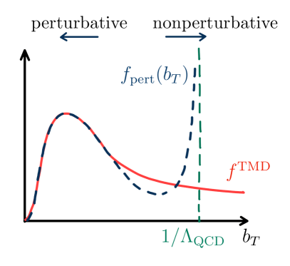
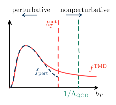
In this paper, we give a set of integral functionals that only require the TMD PDF on an interval as input, where the perturbative description is sufficient, and prove that for large these functionals asymptote to the full momentum-space spectrum. Our construction is based on placing a hard cutoff on the Fourier integral, which makes the contributing regions in space completely transparent, as illustrated in the right panel of figure -659. We then show that the result can be systematically improved by including higher-order contact terms on the boundary. Importantly, by pushing the functional to higher orders in in this way, the effect of nonperturbative corrections of in space can be isolated, and the correction in momentum space can be shown to be linear in the coefficient. This provides a completely model-independent way to compute the leading effect of nonperturbative dynamics on momentum-space quantities, while the evolution and convolution of TMD PDFs can still comfortably be performed in position space at in our setup. We note that a hard -space cutoff on Fourier integrals has previously been considered in refs. [40, 41] as a check on model-specific results, and the setup there amounts to the leading term in our construction. We also show that our construction immediately carries over to the cumulative distribution, and allows us to produce model-independent predictions for the transverse-momentum integral of the TMD PDF. As a byproduct of our analysis, we analyze the scaling of artifacts induced by prescriptions in momentum space, including analyzing schemes whose artifacts scale with different powers or formally fall faster than any power.
Finally, we propose an application to Drell-Yan transverse-momentum () spectra measured at the LHC. We are motivated here by the fact that the most recent measurements by CMS and ATLAS [42, 43] have reached sub-percent precision, making them far more precise than other data sets sensitive to TMD physics. Model-based global TMD PDF fits typically only consider the subdominant experimental uncertainty when computing goodness-of-fit tests, which carries the risk of overconstraining certain flavor combinations and regions. At the same time, the LHC data sets are strongly dominated by perturbative physics . For this reason it is desirable to perform a model-independent fit to LHC data that explicitly incorporates this hierarchy by restricting to the leading nonperturbative effect, which is made possible by our setup. This approach is complementary to model-based fits. As an immediate physics goal, the fit we propose would directly constrain the coefficient in the universal Collins-Soper kernel that governs the evolution of TMD PDFs with energy. Existing model-dependent fits to data [38, 39] and extractions on the lattice [44, 45, 46, 47, 48, 49] both prefer a surprisingly small value for this coefficient, and it would be valuable to confront the extremely precise LHC data with this observation in a model-independent way.
This paper is structured as follows: In section 1.1, we review the status of the relation between TMD and longitudinal PDFs, and point out why considering the cumulative distribution for the TMD PDF is helpful. In section 2 we introduce the truncated integral functionals that allow us to compute Fourier transforms in terms of test function data on , both for transverse-momentum spectra and cumulative distributions. We also discuss the consequences of our construction for prescriptions. In section 3, we apply our setup to the cumulative distribution of a single (unpolarized) TMD PDF and compare the result to the one-dimensional longitudinal PDF. In section 4 we outline the proposed application of our setup to Drell-Yan transverse-momentum spectra at the LHC. We conclude in section 5.
1.1 Review of TMD PDFs and their cumulative integral
An interesting question is how a TMD PDF , which encodes information of both the longitudinal momentum fraction and the transverse momentum , relates to the corresponding collinear PDF , which only encodes the longitudinal information. For definiteness, we will consider to be the distribution of unpolarized partons within an unpolarized hadron or nucleon in this paper. The extension of this review and of our results to polarized distributions is straightforward, and we return to it in section 5. In a naive interpretation of both distributions as probability densities, one might expect
| (1.2) |
i.e., the integral of the more differential TMD PDF should exactly recover the one-dimensional distribution. Using the standard identity , one can equivalently ask about the value of the Fourier transform of the TMD PDF at ,
| (1.3) |
where is the position-space variable conjugate to and .222We will continue to use the same symbol for the unpolarized TMD PDF, its Fourier transform, and the unpolarized collinear PDF in the following as the meaning will always be clear from the arguments or the context.
Indeed, it is easy to work out from their operator definitions [50] that eq. (1.3) is formally satisfied at the level of the bare (unrenormalized) TMD and collinear PDF,
| (1.4) |
where dimensional regularization is used to treat ultra-violet (UV) divergences, and denotes the so-called Collins-Soper scale, which appears due to the need to regulate and subtract rapidity divergences in the construction of the TMD PDF. Specifically, the bare position-space TMD PDF operator is defined as a correlator of parton fields that are separated by some lightlike (longitudinal) distance and by in the transverse direction, and that are connected to each other by a staple-shaped Wilson line extending to lightlike infinity. For , only the lightlike separation remains and the Wilson line collapses onto a single straight path between the two fields, which precisely recovers the operator definition of the collinear PDF. (Similarly, an additional soft component in the definition of the TMD PDF collapses to unity for , and the dependence on the rapidity regulator drops out.) Eq. (1.4) has been explicitly verified to hold in momentum space at one-loop level in ref. [51] by performing the integral in dimensions.
However, after renormalization, the naive result eq. (1.2) must be broken,
| (1.5) |
where is the scale. This is immediately clear from comparing the renormalization group evolution of the TMD and collinear PDF with respect to ,
| (1.6a) | ||||
| (1.6b) | ||||
Importantly, the evolution of the TMD PDF is diagonal both in flavor and momentum fraction , while for the PDF it sums over all flavors and involves a convolution in . Even more strikingly, only the TMD PDF depends on the CS scale through the Collins-Soper kernel , also known as the rapidity anomalous dimension,
| (1.7) |
while the PDF is independent of . More generally, the two-dimensional structure of the renormalization in the TMD case, with the two directions tied together by a closure condition involving the cusp anomalous dimension ,
| (1.8) |
has no analog in the collinear case. Clearly, these observations forbid a simple relation between the TMD and collinear PDF at the renormalized level, and thus break eq. (1.2) in general. Only the renormalized distributions can be extracted from measurements in dimensions, so this is unsatisfactory.
At distances that are short compared to the QCD confinement scale , another relation between the position-space TMD and collinear PDFs exists. In this regime, TMD PDFs obey an operator product expansion in terms of local operators at , i.e., in terms of collinear PDFs [52],
| (1.9) |
Here the matching coefficients carry the dependence on the short-distance physics at the scale . They can be computed perturbatively in terms of and precisely absorb the mismatch in renormalization to the working order in .
Because the total integral of the TMD PDF over all is a UV quantity that one expects to be dominated by large, perturbative momenta, one may be tempted to evaluate eq. (1.9) at to relate the integral to the collinear PDF. In this case, one option is to take while holding the renormalization scale fixed. This expresses the TMD PDF in terms of the PDF at the scale and perturbative corrections starting at . However, the perturbative corrections contain logarithms, , that prohibit setting to compute the total integral. Alternatively, one can evaluate the TMD PDF at and use the evolution equations in eqs. (1.6a) and (1.7) to evolve it back to the overall . In this case the perturbative corrections at the scale actually vanish for due to asymptotic freedom. However, this produces a relation with the PDF at asymptotically large scales , which is hard to interpret.
A physically intuitive way of dealing with these issues, which also produces a practically useful result at finite scales, is to instead consider the cumulative TMD PDF in momentum space up to some finite cutoff, i.e., the distribution integrated over all with , where we can think of as an additional UV cutoff for high-energy modes. This quantity is straightforward to compute in terms of the position-space TMD PDF,
| (1.10) |
Here we inserted the Fourier transform on the first line, performed the trivial integral over the angle of on the second line, resulting in a zeroth-order Bessel function of the first kind. On the third line we interchanged the order of integration to perform the integral, resulting in the first-order Bessel function.
Eq. (1.1) is a typical example of a momentum-space quantity that receives contributions from all , including a long-distance contribution from . Unlike the full integral over all , it depends on a physical scale , which can guide the choice of the overall scales that the TMD PDF is evolved to, and the behavior of the cumulative distribution for large can be studied explicitly. In ref. [53], cumulative distributions of the unpolarized, helicity, and transversity TMD PDFs at were studied for a specific choice of nonperturbative model at long distances (with perturbative results at next-to-leading order), and found to be consistent with their collinear counterparts. A primary goal of this paper, which originally motivated developing the general formalism we present in section 2, is to compute the cumulative distribution in eq. (1.1) at perturbative in a model-independent way in terms of the leading OPE contribution in space and quantifiable corrections.
2 Truncated functionals
Motivated by the physical applications discussed in section 1, in sections 2.1–2.4 we setup a mathematical formalism for systematically obtaining momentum space distributions from an underlying Fourier distribution that obeys an OPE. We then consider the relation to prescriptions in section 2.5 and the nature of an asymptotic series which arises in the construction in section 2.6.
2.1 Setup and assumptions
We consider an integral functional
| (2.1) |
for an arbitrary function that satisfies the following two assumptions:
| (2.2) |
Here we take the sign to mean that there exists a constant and an exponent such that the bound is satisfied for all sufficiently large , and similarly for the first derivative with . In our application, represents the radial momentum spectrum of any position-space function that respects azimuthal symmetry, see the first two lines of eq. (1.1). The physical interpretation of assumption (2) is that correlation functions of parton fields (and their spatial variations) should vanish far outside the hadron. If is not oscillating but becomes monotonic at large , the second part of assumption (2) concerning follows from the first.333In addition, we assume that the original integral in eq. (2.1) exists for any in the sense of an improper Riemann integral. Assumption (2) can be made sufficient to guarantee its existence for any in the Lebesgue sense by requiring , but this is not required for our manipulations below. We also have not made assumptions about the behavior of as yet.
We introduce a cutoff, , which divides the total functional into two parts:
| (2.3) |
where
| (2.4) |
In our applications, should be chosen such that for perturbation theory can be used to compute at short distances, implying that nonperturbative physics only becomes important in the long-distance contribution .
We now focus on developing a formalism to obtain for perturbative momenta . Our goal is to approximate the total functional using only information from the region . To the zeroth order, we define
| (2.5) |
In our application, this ensures that all information about the perturbative domain is already included in the zeroth-order functional, including in particular the resummed dependence on any high scales such as the invariant mass of a color-singlet final state or the Collins-Soper scale.444An alternative would be to construct approximate Fourier functionals in terms of the behavior of the function as , which has previously been considered in the applied mathematics literature [54], see the note added at the end of this manuscript. For our use case, this would require including also the resummed perturbative information only as part of an asymptotic series, and would produce impractical results in terms of the strong coupling and collinear PDFs at asymptotic scales as discussed in section 1.1, so we do not consider this option further. In order to account for the leading contribution from , we compute the integral
| (2.6) |
Starting with the first exact equality, we used integration by parts and the fact that the surface term for vanishes by assumption (2) in eq. (2.1). To obtain the last line we used the asymptotic form of the Bessel function at large to restrict the surface term to the current working order,
| (2.7) |
We further used that assumptions (1) and (2) together imply that is bounded by for all for some suitable , such that we can power count away the remaining integral,555The first inequality is in fact incorrect in general if changes sign in a correlated fashion with . The correct proof proceeds via a Mellin transformation of and , as well as a more explicit evaluation of Bessel integrals in the asymptotic limit, and is given in section 2.2.
| (2.8) |
This scaling again follows from the asymptotic form in eq. (2.7), where the oscillations of the cosine term suppress the value of the integral in eq. (2.8) by one power of .
With this leading correction from at hand, we can define
| (2.9) |
which is an improved approximation of . Importantly, the leading contribution from long distances to the spectrum at perturbative is obtained from the value of the function at the boundary .
2.2 Full proof and higher-order results for the long-distance contributions
We wish to define an asymptotic series of functionals for which have successively improving error terms for . In these functionals, we aim to only use information about the test function from the region , but systematically account for the contributions from by including higher-order surface terms. In order to prove the form of the surface terms up to and including order , we need the function to satisfy stronger assumptions:
| (2.10) |
Assumption again follows from the simpler assumption if and its derivatives become monotonic power laws (or exponentials) for sufficiently large . The reverse is always true, i.e., follows from assumption for all by bounding the iterated integral.
Mellin transform.
Our strategy is to decompose in terms of basis functions of the form , with a continuous parameter, to make the power counting of individual terms transparent. This amounts to taking the Mellin transform,
| (2.11) |
so that the function can be written using the inverse Mellin transform
| (2.12) |
Here the real part of the chosen contour satisfies
| (2.13) |
Together with bounded variations of , eq. (2.13) is sufficient for the existence of the Mellin transform and its inverse, see e.g. theorem 28 in ref. [55]. Both conditions are satisified by assumption for and . Below we will need , and this is why we required a strict inequality . Note that assumption in the same way guarantees the existence of the (inverse) Mellin transform for all derivatives with . The relation is particularly compact for repeated derivatives with respect to ,
| (2.14) |
Bessel integral for a single power.
To make contact with the Bessel integral above a cutoff , let us consider
| (2.15) |
The integral exists for all complex parameters with and is the hypergeometric function. To obtain the last equality we used the asymptotic expansion of for [56], which generalizes the asymptotic expansion of the Bessel function in eq. (2.7). The coefficients are polynomials in of order and are collected in appendix A.1 up to . The first few coefficients read
| (2.16) |
Assembling the long-distance contribution.
The above definitions allow us to compute the long-distance contribution to in terms of the Mellin transform of ,
| (2.17) |
On the second line, we plugged in the inverse Mellin transform. On the third line, we changed the order of integration and used the definition of in eq. (2.2), which is justified because the integral exists for each power with along the contour individually. Crucially, on the last line we performed the asymptotic expansion of and pulled the phase and the additional power suppression of each term out of the Mellin integral. Note that naively, the scaling of the error term would be because the remaining integral scales as . However, the coefficient of this additional factor of , which is encoded in , is unrelated to and instead comes from the power law bounding the function.
We now use that the coefficients are polynomials in , and evaluate the remaining Mellin integral in eq. (2.2) using eq. (2.14), which turns powers of into repeated derivatives on the boundary,
| (2.18) |
This is our key result in this section: At each order in the power counting, the long-distance contribution can be expressed entirely in terms of the test function and its derivatives evaluated on the boundary. Adding the short-distance contribution , we define
| (2.19) |
We call these functionals of “truncated functionals”, referring both to the truncation of the integral and of the asymptotic series. We reiterate that the truncated functional approximates up to
| (2.20) |
Writing out the derivatives with respect to , we find for the first few coefficients , as required for :
| (2.21) |
The first term reproduces the given in eq. (2.9).
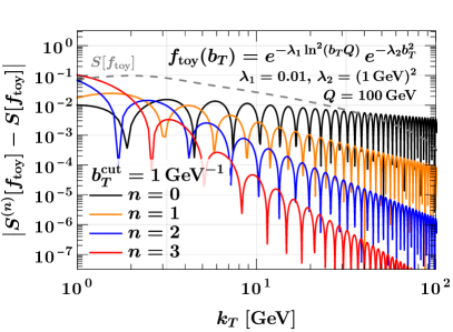
In the left panel of figure -658, we test the asymptotic expansion for a simple, but physically relevant toy test function
| (2.22) |
Here the term is a proxy for the perturbative Sudakov exponential appearing in TMDs, and the term is a proxy for a nonperturbative contribution. The full spectrum is shown by the dashed black line, while the solid lines display the absolute value of the error left over from subsequent approximations by our truncated functionals . We clearly see that compared to the full spectrum , the error term of the truncated functional exactly follows the expected scaling given by eq. (2.20) and improves as we go to higher .
2.3 Marrying the OPE to the truncated functionals
Consider a function which, apart from satisfying assumptions and in eq. (2.2), can also be written in terms of an asymptotic series expansion,
| (2.23) |
where and has at most a logarithmic dependence on . In our physics application, the above asymptotic series arises from an operator product expansion (OPE) that expresses the matrix element of a nonlocal operator in terms of local operators suppressed by increasing powers of a low physical scale . We keep the Wilson coefficients of the local operators that carry the non-analytic dependence on implicit in . The OPE may in addition have a finite radius of convergence , such that the limit exists for all , but we do not require this in the following. In physical terms this means we allow for the violation of quark-hadron duality [57] e.g. by terms . For simplicity we will also refer to the first OPE term as the “perturbative” part of , since in our application it can be evaluated using pertubation theory and known, simpler matrix elements.
Suppose we know the OPE up to order , which means that the leading error term is . We now show that in this case, we can approximate the total functional using the truncated functionals with only the known OPE terms as input.
For simplicity let us first assume that only the leading perturbative term is known, and that the next term is suppressed by two powers of , i.e., , as is often the case. After the Fourier transform, we have corrections
| (2.24) | ||||
where on the first line we account for the correction from truncating the functional, and on the second line the three types of power corrections account for the correction from truncating the OPE. We see that the third class of power corrections, which is a combination of the neglected in the surface term and the error term of the functional, is suppressed more strongly than the intrinsic OPE correction for functionals with sufficiently high order . In particular, there are no corrections of , and we give a short proof of this statement for the general case below.
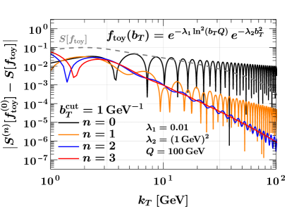
For an illustrative example of the effect of truncating the OPE under the functional, see the right panel of figure -658, where we test eq. (2.24) with the toy function in eq. (2.2). We put only the leading perturbative term into the truncated functionals, where
| (2.25) |
We see that increasing the order of the truncated functionals stops improving the result around the quadratic order, because they become subleading to the intrinsic “nonperturbative” OPE correction . This means starting at , the error term of the truncated functional is “stuck” at a quadratic power law, allowing us to identify the leading OPE correction directly in momentum space. In section 4 we will exploit this to propose a model-independent method to constrain nonperturbative dynamics from momentum-space data.
Now for the more general case, suppose we know the OPE up to order , i.e. . We need to compute to find the leading momentum-space error term from the truncation of the OPE. Note that for itself, the full functional does not exist, since with at large . However, we can construct a function that agrees with for all but also satisfies assumptions and in eq. (2.2), e.g. by applying an exponential prescription (see section 2.5) to and multiplying the result with a similarly constructed exponential model. Then we have
| (2.26) | ||||
where in the last equality we have used that is independent of , and thus by dimensional analysis can only yield the intrinsic OPE correction . We see that the second term, which accounts for corrections in , is suppressed compared to the first when without having to assume that . Combined with eq. (2.20) we have
| (2.27) |
Note that each term is individually well defined despite the growth of the integrand at large , since it only involves a compact domain. We could therefore exploit that the truncated functionals act linearly on the terms in the OPE, which enabled us to move the sum out of the functional. Specializing to and as above, we recover eq. (2.24), where power corrections of are absent and the third class of power corrections is suppressed for .
Eq. (2.27) is the main result of this section. It allows us to compute a momentum-space quantity (a TMD spectrum) at large momenta purely in terms of our perturbative knowledge of the position-space OPE at short distances, without having to place any assumptions on the long-distance behavior. The approximation is fully controlled and can be systematically improved by either pushing the knowledge of the OPE to higher orders , or by carrying surface terms in the truncated functional to higher orders . In particular, higher-order terms in the OPE are mapped to momentum space order by order in the power counting thanks to the linearity of the functionals.
2.4 Extension to cumulative distributions
In physics applications, we are often interested in a slightly different, but related integral functional,
| (2.28) | ||||
which corresponds to the cumulative distribution over all momenta in an azimuthally symmetric position-space function , see eq. (1.1).
We may again introduce a perturbative cutoff and divide the into and analogous to eq. (2.1), and apply the same procedure described in section 2.2 to derive a series of functionals that asymptote to for large ,
| (2.29) | ||||
These truncated cumulative functionals approximate up to an error term given by
| (2.30) |
The expressions above are analogous to eqs. (2.2) and (2.20) for the spectrum. We give the first few coefficients needed to construct with eq. (2.29) for :
| (2.31) |
Higher-order functionals can be computed using the coefficients given in appendix A.2. Restricting the input to the functionals to the first orders in the OPE of the test function at small , we have
| (2.32) |
which should be compared with eq. (2.27). Once again the linearity of the functional was used to pull the sum outside the functional.
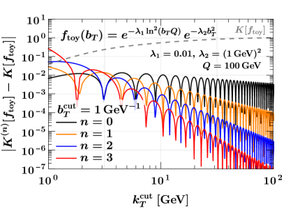
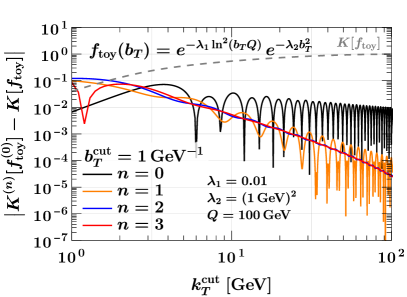
The left panel of figure -657 shows that the cumulative functionals exhibit the expected power-law scaling of error terms for the toy function in eq. (2.2). In the right panel of figure -657 we again restrict the input of the functionals to the leading term at small , , and compute the difference to the full result . Starting from , we find that the intrinsic correction results in a power-law behavior of this difference, as expected. Note that for the cumulative distributions, rather than is already sufficient to expose the quadratic behavior of the intrinsic OPE correction.
2.5 Consequences for prescriptions
In the -space formalism of TMD PDF modeling, one often introduces a function to shield the Landau pole in the perturbative computation, as presented in eq. (1.1) in the introduction. Two common prescriptions in the literature are the Collins-Soper prescription [25] and the Pavia prescription [26]:666We have taken in the original prescription, which as argued in ref. [26] only amounts to a modification in the UV (beyond the validity of TMD factorization). This allows for a more direct comparison to other models which have .
| (2.33) |
When evaluating at and expanding for , we have
| (2.34) |
where we note that the first subleading terms in the series differ, with and scaling respectively.
We can formally assess the momentum-space effect of the residual dependence by applying our truncated functionals at sufficiently high orders to . For example, using with for CS and for Pavia, we can show using eq. (2.27) that the leading correction terms in eq. (2.5) carries over to momentum space with the scaling expected from naive power counting, where for the Collins-Soper prescription and for Pavia. As we push to higher orders of , we can identify the scaling of the leading corrections in momentum space using a plot similar to figure -658.
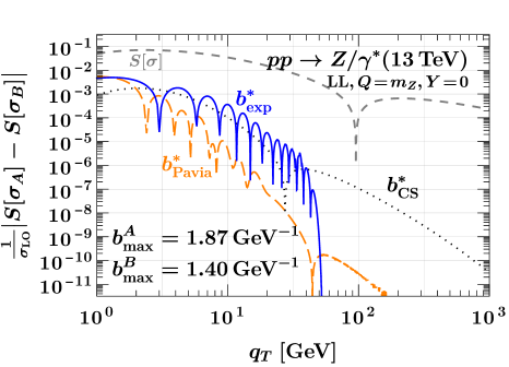
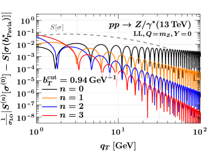
To test the impact of different choices we consider where is the leading (double) logarithmic (LL) inclusive differential cross section for at the LHC, normalized to the tree-level cross section. We use the LL solution of the running coupling starting from , which exhibits a Landau pole at . For numerical stability, we keep the scale of the PDFs in the resummed prediction fixed at the high scale , which is an NLL effect. In figure -656, we show the scaling of the difference between using and in momentum space for different models. We also include the value of an individual (dashed gray curve) using with as reference. All curves are normalized to the Born cross section . We consider the behavior of (dotted black) and (dashed orange), as well as an exponential prescription (solid blue) defined as
| (2.35) |
The benefit of the prescription is that it does not introduce additional powers beyond those predicted by the OPE. In addition, for any function including the prescription is exactly equal to the input function, . In our numerics we have chosen , which is the largest value allowed such that is still monotonic. We observe that the scaling of the ambiguity of the CS and Pavia prescriptions both stabilize to their corresponding power law ( and , respectively), as expected from our analytic arguments below eq. (2.5). For our newly introduced prescription we see that the scaling indeed falls off faster than any power for large enough , as expected. Unfortunately, we find that the coefficient of the exponentially suppressed ambiguity is rather large, so that the practical usefulness of the prescription, beyond the formal improvement of preserving the OPE coefficients, may be limited.
We note that these conclusions also apply when the prescription is only implemented through the choice of boundary scales in resummed perturbation theory (a so-called local prescription), rather than also substituting the (global) kinematic dependence of the factorized cross section by , which is needed e.g. in the presence of additional measurements on soft radiation to preserve refactorization relations for the relevant matrix elements [28]. It also applies to the choice of TMD PDF boundary scale with at which the OPE of the TMD PDF is performed in ref. [38], and which we expect to translate to linear power corrections in momentum space. In either of these cases, the total derivative in eq. (2.5) is replaced by partial derivatives with respect to the relevant scale(s) , but the power-law scaling of the artifacts induced by the prescription still follows from expanding the relevant profile scale function for small , and will carry over to momentum space in the way described above. We also note that in both the setup of ref. [28] and ref. [38], the modification of the function occurs in a region where left-over fixed-order logarithms of may be large, so the dependence is not guaranteed to decrease as the perturbative order increases.
2.6 Series stability near the Landau pole
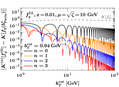
As a final check on our setup, we consider the stability of the truncated functional series when applied to a test function that exhibits an actual Landau pole beyond the support of the integral functionals. This is relevant because in the presence of a pole at , we generically expect the derivatives of the test function to grow factorially, e.g.,
| (2.36) |
As the highest derivative enters the truncated functional at order with coefficient , see appendix A, this factorial growth feeds through into the result for the functional. We use the same numerical setup as in the previous setup, evaluating a single TMD PDF (or the Drell-Yan cross section) at leading-logarithmic (LL) order with a Landau pole at , but without applying any prescription in this case. We continue to fix the PDF scales at the high scale for the TMD PDF and at for the cross section, for numerical stability.
In figure -655 LL results for the cumulant of a single quark TMD PDF (left) and the Drell-Yan transverse momentum spectrum at the LHC (right) are shown. In both cases, while the overall coefficient of the error term is substantially larger than for the test function in figures -658 and -657, we still observe a stable improvement in the error term when going to higher orders in the functional. This indicates that at least up to the order we consider here, the Landau pole does not deteriorate the quality of the asymptotic approximation.
3 Calculating the TMD PDFs and their cumulative integral
3.1 Evolution and operator product expansion of the TMD PDF
The dependence of the TMD PDF on the renormalization scale and the CS scale is governed by the evolution equations in eqs. (1.6a) and (1.7). They can be solved in closed form to evolve the TMD PDF from some initial values to ,
| (3.1) |
Here we have chosen the evolution path as . We can in particular use eq. (3.1) to evolve the TMD PDF away from the canonical boundary condition at which the TMD PDF is a single-scale quantity and thus free of large logarithms to all orders in perturbation theory and in . In explicit numerics we choose the canonical boundary scales as
| (3.2) |
where we include a conventional numerical coefficient with the Euler-Mascheroni constant. We will also refer to this boundary condition simply as the “intrinsic” TMD PDF.777Other choices of the boundary scale and evolution path are also possible; for examples relevant to recent TMD PDF extractions see e.g. ref. [26], where is held fixed at a low scale , or refs. [27, 58], where the boundary scales are set by a recursive procedure taking the (perturbative and nonperturbative) rapidity anomalous dimension as input. We stress that while the result for the rapidity anomalous dimension is unambiguous, different choices of amount to moving nonperturbative contributions proportional to the rapidity anomalous dimension in and out of the intrinsic TMD PDF.
We are interested in values of where the TMD PDF and the rapidity anomalous dimension obey an operator product expansion [52, 18, 59, 60, 61],
| (3.3) |
with . Most often the terms with odd vanish. The anomalous dimension in eq. (1.6a) is a UV quantity and does not receive nonperturbative corrections, so we simply wrote down the OPE at the overall scale , which does not need to be equal to . On the other hand, the evolution mixes powers in the expansion. Specifically, for the first nonvanishing orders in a TMD PDF with , ,
| (3.4) | ||||
The structure of at higher orders is relatively well understood. The leading perturbative term is known to three loops [62, 63, 64], and also contributes the overall additive renormalization of in eq. (1.8). Recently, ref. [61] demonstrated that the contribution can be related to a gluon vacuum condensate. Assuming a tree-level Wilson coefficient and ignoring the running of the condensate as in ref. [61], is a single fixed number with units of .
The entries of the OPE for a TMD PDF in general are given by multiple convolutions of perturbative Wilson coefficients, which encode the logarithmic dependence as , and higher-power matrix elements that provide the power suppression by . The leading term for the unpolarized quark or gluon TMD PDF takes the form
| (3.5) |
where is the collinear PDF, are the matching coefficients, and the sum runs over all partons . The linear correction to the unpolarized TMD PDF vanishes by azimuthal symmetry [59, 60].
Not much is known about the OPE of the unpolarized TMD PDF beyond the linear order. A subset of terms that multiply the leading-twist collinear PDF was determined to all powers in and at tree level in in ref. [65]. These correspond to target mass corrections to the TMD PDF because only the hadron (or nucleon) mass can provide the power suppression at in this case; nevertheless, they only constitute a subset of the full OPE at any given order in .888Interestingly, we find that the Fourier transform of the result in ref. [65] for the unpolarized TMD PDF in their eq. (4.13) actually exists (in the distributional sense), with the cumulative distribution given by (3.6) In particular, the dependence of the TMD PDF in this approximation is cut off at , which has a simple interpretation in terms of the remnant of the struck hadron consisting of on-shell states, i.e., with the hadron and the parton momentum. It would be interesting to investigate whether the results of ref. [65] for spin-dependent TMD PDFs can be understood in a similar physical way. For the purposes of this paper, we will consider the most general form that the quadratic correction can have based on the RG properties,
| (3.7) |
where has units of . To see this, recall that the dependence of the quadratic term has to be that of the leading-power one, which motivates writing it as a product involving . By eq. (3.4), the remaining coefficient is renormalized as
| (3.8) |
Evaluating at our reference boundary scale , we are left with a function of the flavor , , and . As for the rapidity anomalous dimension, we assume leading-order Wilson coefficients and ignore the running of the higher-twist matrix elements and soft condensates from to . (The running in general would dress the leading scaling with an anomalous exponent, and similarly for Wilson coefficients that start at .) This leaves us with a function of a single variable for each flavor.
Combining both sources of nonperturbative corrections and fixing , we have
| (3.9) |
where we defined as a shorthand. We also absorbed the leading-power rapidity evolution factor into , which evolves it back to the overall . Importantly, the impact of on the evolved TMD PDF is linear at this order thanks to the power expansion of the evolution kernel. This is crucial, because our truncated functionals are precisely set up to act linearly on terms in the -space OPE, so we will be able to move the coefficient out of the Fourier transform. This setup will allow us to study the linear impact of the OPE coefficients and on momentum-space observables, either as an uncertainty on the transverse-momentum integral of a single TMDPDF in section 3.2 or as a signal template for our proposed fit to data in section 4.
3.2 Approximating the cumulative TMD PDF with truncated functionals
The cumulative integral of an azimuthally symmetric TMD PDF over ,
| (3.10) |
can be computed in terms of the -space TMD PDF with exactly the functional we have defined in eq. (2.28). At large we can therefore use the formalism described in section 2 to approximate the cumulative distribution of a single TMD PDF in order to eventually study its normalization.
Thanks to the OPE eq. (3.1), we can calculate the resummed leading OPE term in space in terms of collinear PDFs. We use the numerical implementation of the matching coefficients and anomalous dimensions in SCETlib [66] as also used in ref. [67]. More details on our evolution and resummation setup for are given in section 3.3. We evaluate at N3LL order, which requires the two-loop matching coefficients for the TMD PDF [68, 69, 62], the three-loop collinear quark anomalous dimension [70], the perturbative Collins-Soper kernel to three loops [63, 64], and the four-loop cusp anomalous dimension [71, 72], We assume active flavors in the matching coefficients and throughout the TMD evolution. We use the CT18NNLO PDF set [73] as provided by LHAPDF [74] together with four-loop running [75, 76] of the coupling starting from .
Applying our truncated functionals to the leading OPE term, , we obtain a purely perturbative baseline for the -cumulative TMD PDF. In the following we use , which we find to be numerically stable and sufficient for our purposes in this section. We set such that all scales in the resummed TMD PDF stay above , i.e., well away from the Landau pole. We use standard adaptive integration tools to evaluate , and evaluate the required derivatives for the surface terms in a numerically stable fashion using Lanczos’ method of differentiation-by-integration [77, 78]. We find it convenient to change variables to in the test function before differentiating at , which both improves the numerical stability and makes it straightforward to push the implementation to high orders using the coefficients in appendix A. When needed, e.g. when comparing to explicit models, we perform Bessel integrals over the full range using a double-exponential method for oscillatory integrals [79, 80, 81] as implemented in SCETlib [66].

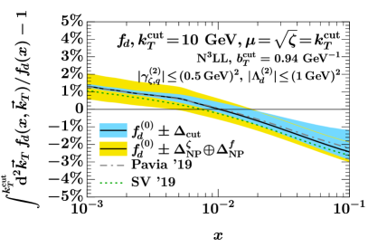
We can now compare our approximated cumulant to the collinear PDF in order to quantify the deviation from our naive expectation eq. (1.2). In the left panel of figure -654, we show the normalized deviation of from the collinear PDF as a function of the transverse-momentum cutoff while keeping fixed. In the right panel of figure -654, we show the same deviation from the collinear PDF as a function of the momentum fraction , while keeping fixed. In both cases we set . We find that the central value of our prediction (solid black) only deviates from the collinear PDF at most at the percent level for , and for is essentially equal to the PDF for . For () we find a small positive (negative) deviation.
We consider two sources of nonperturbative uncertainty on our result in this section, deferring an estimate of perturbative uncertainties to section 3.3. The first uncertainty component , shown in blue in figure -654, is estimated by varying from to . Since the residual dependence is intrinsically beyond our working order, it parametrizes our ignorance of the long-distance behavior of the TMD PDF.
The second source of nonperturbative uncertainty is the behavior of the TMD PDF at short to intermediate distances , where the TMD PDF is governed by the OPE. We can assess the uncertainty related to this region in a fully model-independent way by treating the quadratic OPE coefficients and in eq. (3.9) as unknowns and propagating them into the cumulative distribution in momentum-space by injecting the corresponding OPE term into our truncated functional. Importantly, the action of the functional on each term in brackets in eq. (3.9) is linear, i.e., we have, suppressing the arguments of the TMD PDF,
| (3.11) |
The impact of and on the predicted transverse-momentum integral of the TMD PDF is therefore also linear, including their a priori unknown sign. While we consider simple estimates of the unknown coefficients here to demonstrate the method, their linear impact makes it completely straightforward to update the uncertainty estimate (or the central value) to any determination of the coefficients from model-based global fits to experimental data or a lattice calculation. It also makes the uncertainty very cheap to evaluate since the three functionals in eq. (3.11) only need to be evaluated once, rather than having to perform a Fourier transform for each choice of model parameters.
For definiteness, we consider a variation of independent of , which yields an uncertainty . We stress again that this assumption is straightforward to relax point by point in the right panel of figure -654 by a trivial rescaling. To estimate the uncertainty due to higher OPE corrections to the CS kernel, we adopt a very conservative range of , yielding the second OPE-related uncertainty component ; recent model-based global fits [38, 39] and the condensate-based estimate from ref. [61] all point to substantially lower values of . For readability, both nonperturbative uncertainty components are added in quadrature in figure -654, , and are shown in yellow.
We find that for the integral of the TMD PDF is fully compatible with the collinear PDF for all values of already within the nonperturbative uncertainties, while for general the nonperturbative uncertainty alone only covers part of the difference. Both uncertainty components quickly decrease as increases, as expected from their respective power counting.
Finally we also include in figure -654 the cumulative TMD PDF as predicted by the SV [38] and Pavia [39] model-based global TMD fits. We use arTeMiDe [82] to evaluate the SV fit result in space, assuming the best-fit N3LL model parameters from ref. [38], and use our in-house setup to perform the Bessel transform. In the case of the Pavia global fit, we encounter the difficulty that our treatment of quark mass thresholds is different from the one in the NangaParbat [83] native fit code, where the number of active massless flavors is changed discontinuously as a function of . This has a very large effect at large (about at , and up to at ), which distorts the comparison of the genuine nonperturbative effect. For this reason we have set up an independent implementation of the Pavia fit model, using the central replica of the N3LL Pavia fit as provided in ref. [84], and combined it with our implementation of in SCETlib evaluated with the prescription of ref. [26], with as in eq. (2.5). We have verified that above the bottom-quark threshold, our result for is within a permil of the result returned by NangaParbat for .999The discrepancy to arTeMiDe in the perturbative region, or when turning off the arTeMiDe nonperturbative model, is somewhat larger, at roughly half a percent. We attribute this to the different choice of boundary scale within the so-called prescription used in arTeMiDe. Both global fits support our conclusion that the deviation from the naive expectation is within percent level. In particular, they are compatible with our perturbative baseline well within our estimate of the nonperturbative uncertainty, indicating that our model-independent approach is sound.
In figure -648 in appendix B, we show the same plots as in figure -654 for other light quark flavors (, and ). We find that the results are very similar to the discussion for the down quark in this section.
3.3 Perturbative uncertainty
Since we rely on the accuracy of the perturbative input , it is also important to consider the theoretical uncertainty from the truncation of perturbation theory. We estimate the perturbative uncertainty at different resummation orders by varying the boundary scales entering the evolved TMD PDF. As described below, we adapt the variation procedures developed for the resummed spectrum in ref. [67], noting that for our case there are some simplifications compared to the original setup.
The TMD PDF at generic , which may be parametrically separate from , is a multi-scale problem. One way of treating it in resummed perturbation theory is to evaluate it at , where it is free of large logarithms, and use eq. (3.1) to evolve it back to the overall . The uncertainty estimate in that case could be estimated by varying the boundary scales .
Alternatively, one can consider a factorization of the TMD PDF at generic into purely collinear and purely soft matrix elements,
| (3.12) |
which individually are single-scale problems and feature an additional rapidity renormalization scale . In the SCET literature, these matrix elements are known as beam and soft functions.101010We use the exponential regulator of ref. [85] that renders the overlap subtraction between the beam and soft function scaleless, see the discussion in Section 2 of ref. [33]. More details on rapidity regulators can be found in Appendix B of ref. [33]. In this setup, the running in from the canonical beam scale to the soft scale resums the large logarithms of . For the central prediction, where all scales are set exactly to their canonical values, this is exactly equivalent to running the TMD PDF as a whole as described below eq. (3.1). The two approaches differ, however, once the possible variations of the boundary scales are considered. In particular, the factorized form in eq. (3.12) allows for varying all of and individually, providing a more robust estimate of the perturbative uncertainty that makes use of the full available information about the factorization structure. (In practice, to estimate the perturbative uncertainty on the leading OPE term we of course only need to evaluate eq. (3.12) at leading power in .)
The procedure of ref. [67] is to consider the variations111111Note that in ref. [67], hybrid profile scales were used to turn off the resummation as to implement the matching to power corrections of (also known as the term). For a single TMD PDF, which is already one of the objects appearing in the leading-power factorization, these corrections are absent, so we can keep the resummation on everywhere. This amounts to taking in the profile scales in ref. [67].
| (3.13) |
where the four variation exponents can be . The central scale choices are given by . A priori there are 80 possible different combined variations of the . Since the arguments of the resummed logarithms are ratios of scales, e.g. , some combinations of the ’s lead to variations of these arguments by more than the conventional factor and are therefore excluded, leaving us with 36 different combined scale variations. We calculate for each of them and then take the maximum envelope as our estimate of the perturbative resummation uncertainty .
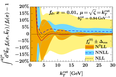
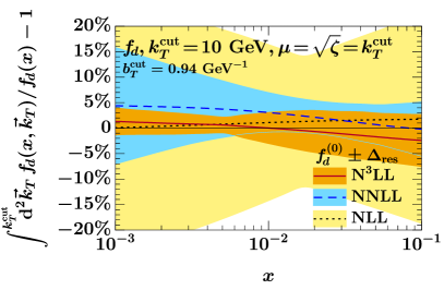
In figure -653 we show for the cumulative TMD PDF calculated at NLL, NNLL, and N3LL as a function of and of . The parameter choices are the same as in section 3.2. When we calculate the perturbative to higher resummation orders, we see a convergence of the bands, giving us confidence in the robustness of the uncertainty estimate. The central values at all resummation orders are within a few percent from the collinear PDF for , and the cumulative TMD PDF is compatible with the collinear PDF well within the perturbative uncertainty for all and . Notice that the perturbative uncertainty in figure -653 is much larger than the nonperturbative uncertainties shown in figure -654.
Figure -647 in appendix B shows the same plots as in figure -653 for other light quark flavors. The results are once again very similar to the discussion for the down quark in this section.
3.4 Impact of evolution effects
In the discussions above, we have chosen , which is the natural scale choice such that the left-hand side of eq. (3.10) only depends on one scale . In this section, we would like to consider how evolution away from these natural scales impacts our conclusion about the transverse-momentum integral of TMD PDFs.
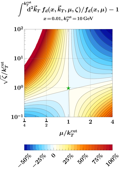
In figure -652, we show the normalized deviation of the cumulative TMD PDF at from the collinear PDF as a function of both the renormalization scale and the CS scale . We find that, in the vicinity of the natural scale choice , our conclusion is robust against evolution effects and the deviation remains within percent level. In particular, along the line of fixed , we find that the evolution is negligible. This has the intriguing physical interpretation that the evolution of the momentum-space TMD PDF is only a shape effect, i.e., while it changes the shape of the TMD PDF at low , the transverse-momentum integral stays the same and is determined by collinear physics.
When we move away from , sizable deviations from the collinear PDF arise from the large logarithm induced by the cusp anomalous dimension. To further understand this, consider the evolution path . Since the evolution at fixed is only a shape effect, the first evolution step only changes the transverse-momentum integral of the TMD PDF within a few percent. In the second step, however, the evolution factor resums large double logarithms of the form
| (3.14) |
where the ellipses indicate single logarithms and is the one-loop coefficient of the cusp anomalous dimension. Thus the effect of the evolution is stronger for a larger ratio of at the starting point, which is responsible for the saddle point structure observed in figure -652. This confirms the initial observation in section 1 that an equality between cumulative TMD PDF and collinear PDF cannot hold at all scales due to the different renormalization, which resums double logarithms in the case of the TMD PDF. Nevertheless, a relation in the vicinity of is not in contradiction with the renormalization, and is in fact observed in figure -652 to also extend to parametrically separate values of at fixed .
We conclude that, even when we take the evolution effects in the vicinity of into account, our intuitive result that the transverse-momentum integral of TMD PDF is within few percent of the corresponding collinear PDF remains robust.
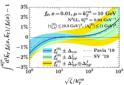
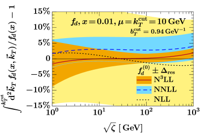
It is also interesting to look at the evolution alone. In figure -651, we show the deviation of the transverse-momentum integral of a TMD PDF from the collinear PDF as a function of , while keeping and fixed. In the left (right) panel of figure -651, we consider nonperturbative (perturbative) uncertainties , , and () as described in section 3.2 (section 3.3). We see that the perturbative uncertainties from resummation still dominate over the nonperturbative uncertainties described in section 3.2, but reduce as the TMD PDF is evolved to very high energies . The uncertainty (light blue in the left panel) likewise reduces at large , which is expected as the Sudakov suppression of the long-distance region increases, while the (light green) component comes to dominate the total OPE uncertainty (yellow) both at very small, , and very large , i.e., far away from the natural choice .
Figure -646 and figure -645 in appendix B show the same plots as in figure -652 and figure -651 for other light quark flavors. The results are very similar to the discussion for the down quark here. Once again, remarkably good agreement is found for the integral of the TMD PDF and the collinear PDF with the most natural choice for fixing the evolution scales.
4 Model-independent constraints on nonperturbative physics from data
4.1 Outline of the method
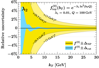
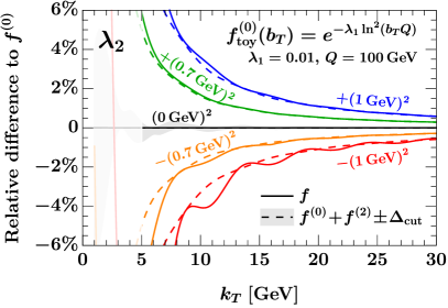
In the previous section we used the action of our truncated functionals on the quadratic terms in the OPE to provide a model-independent estimate of nonperturbative uncertainties in cumulative TMD PDFs, treating the coefficients as unknowns. This approach of course remains valid for transverse-momentum cross sections. In this section we explain how information on nonperturbative contributions to cross sections can be isolated, illustrating the steps with the toy model in eq. (2.3). In the left panel of figure -650 we show the transverse-momentum spectrum , where we vary the quadratic coefficient within two different ranges of values, as indicated by the yellow bands. We normalize the impact of to a baseline given by the third-order truncated functional applied to the purely “perturbative” component of the function, . We see that the relative impact of is slightly larger than expected from power counting, e.g., it amounts to at for , which we attribute to the falloff of the spectrum beyond the Sudakov peak that is present also for this toy function.
There is, however, a second way to make use of the linear impact of the quadratic OPE coefficients in our setup when the transverse-momentum spectrum is known from data. In this case, a fit to data may be performed treating the OPE coefficients as a “signal” that can be discriminated from the purely perturbative “background” in a model-independent way. Importantly, since the action of the functional is linear, the fit template for the signal only needs to be computed once and can then be trivially rescaled in the fit, e.g. for our toy function in eq. (2.3),
| (4.1) |
where (the combined “OPE” coefficient at the quadratic order) would be the parameter of interest in the fit. We illustrate this approach in the right panel of figure -650, where the dashed lines are the combined fit template for signal and background for different values of . To generate illustrative “data” (solid lines) for , where the original toy function in eq. (2.2) has a divergent Fourier transform, we modify it as
| (4.2) |
where is unchanged. This ensures that the full integral exists for all while maintaining for either sign. We see that the fit template predicted by the truncated functionals closely follows the mock data in figure -650 for all values of and , with the exception of where our modification in eq. (4.2) results in a strong modification of at large distances, leading to a larger oscillatory error term.
4.2 Proposed application to LHC Drell-Yan data
We next outline an application of our method aimed at constraining nonperturbative corrections using LHC data for the Drell-Yan process, , which are some of the most precise data taken at the LHC to date [42, 43]. At leading power in , but to all orders in , the fiducial cross section differential in the dilepton transverse momentum reads
| (4.3) |
where is the Born phase-space for a dilepton pair with total invariant mass and total rapidity , where the lepton is scattered at a polar angle measured in the Collins-Soper frame [86]. (For the Born kinematics considered here, the Collins-Soper frame coincides with the frame boosted by along the beam axis from the lab frame.) In eq. (4.3), we have made power corrections in explicit, but will suppress these in the following. The acceptance of the fiducial volume evaluated on Born-level kinematics with is denoted by . For a typical fiducial volume at the LHC,
| (4.4) |
where define an invariant-mass bin (e.g. around the resonance) and the lepton transverse momenta and pseudorapidities are required to be within the fiducial detector volume. (The extension to bins of rapidity as e.g. in ref. [42] is trivial.) In eq. (4.3) we have used our shorthand for the integral functional in eq. (2.1) that performs the Fourier transform from position space. It acts on the factorized unpolarized cross section in position space [87],
| (4.5) |
where is the Born cross section for the hard production process that includes the -dependent lineshape, is the so-called hard function that encodes virtual corrections to the hard process,121212Here we have neglected singlet contributions to the quark axial and vector form factors starting at and , respectively, where the initial-state flavors do not couple directly to the boson. These contributions are straightforward to restore for the high-precision background prediction, but can safely be neglected in the recasting step for a measured coefficient that we outline below. and the sum runs over all contributing quark flavors. The two TMD PDFs on the right-hand side of eq. (4.5) are evaluated at
| (4.6) |
with the total center-of-mass energy of the proton-proton collision. Inserting eq. (3.9), it is straightforward to give the factorized unpolarized cross section to ,
| (4.7) |
where .
If we try to use eq. (4.2) in eq. (4.3) directly, we face a problem commonly encountered in extractions of (TMD)PDFs, namely that the flavor and dependence of the model, in this case the , only enters under the sum over flavors and the integral over hard phase space, and enters in different ways for different center-of-mass energies. Resolving this usually requires writing down a model-specific ansatz and performing a global fit to a large data set at once to constrain it. We now demonstrate that thanks to the linear impact of the OPE contribution to the TMD PDF at quadratic order, its and flavor dependence can be condensed into a single aggregate coefficient per fiducial volume that can be determined by a two-parameter fit with to the data in that single fiducial volume. We also demonstrate that the measured central value, or limits, for can be straightforwardly recast and checked against specific models by performing a simple weighted tree-level integral over the model function.
To set up some more notation, let us define the total fiducial cross section in space,
| (4.8) |
which is possible because we consider the -independent Born acceptance . We then simply have . Our goal in the following is to break down the quadratic contribution to into two terms with a single, overall coefficient each encoding the nonperturbative physics. This is straightforward for the contribution from the rapidity anomalous dimension,
| (4.9) |
because it is flavor independent and thus only involves a simple logarithm of as an additional weight under the hard phase-space integral over the leading-power cross section. To cast the contribution from the intrinsic TMD PDFs into the same form, we define
| (4.10) |
where to match eq. (4.2) the average coefficient must be defined by
| (4.11) |
The fact that it is simply a ratio of (weighted) leading-power integrals is due to the linear impact of on the cross section point by point in phase space. It is always possible to evaluate the right-hand side of eq. (4.11) for a given model to compare it to a measured value of .
However, given the expected sensitivity to at the LHC (discussed below), we anticipate that the right-hand side of eq. (4.11) will only be required at relatively low accuracy to compare (limits on) to models. In this case, we can neglect logarithmic dependence across the bin in several places to a good approximation, namely in the hard function boundary condition, in its evolution down to the TMD PDF scale , and in the leading-power rapidity evolution factor. As a consequence, all of these terms cancel in the ratio since we can effectively evaluate them at some reference value of within the bin. We can also evaluate the intrinsic leading-power TMD PDF at NLL, leaving only
| (4.12) |
Both the numerator and the denominator are a straightforward tree-level integral of collinear PDFs against the line shape and the acceptance, with an additional weight of in the numerator. The residual dependence on can be used as a handle on the theory uncertainty during this recasting step, where should be picked near the -space Sudakov peak, .
In total, our -space input for a given fiducial volume integrated over hard phase space reads
| (4.13) |
Applying our truncated functionals at order and exploiting their linearity, we have,
| (4.14) |
We now illustrate the numerical impact of the two remaining nonperturbative parameters, working at fixed and and applying no fiducial cuts for simplicity, i.e., we consider
| (4.15) |
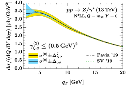
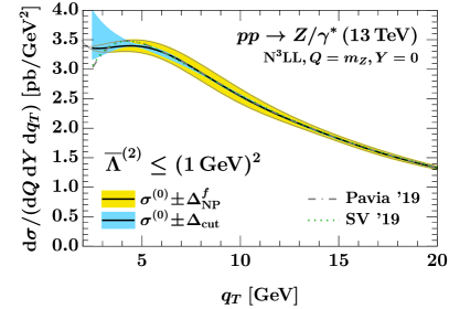
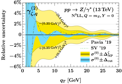
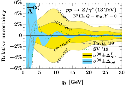
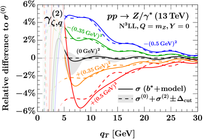
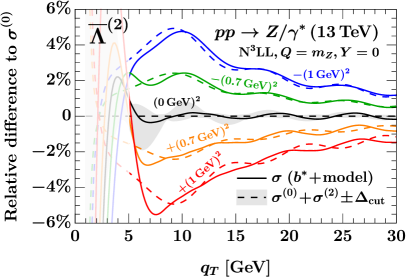
The recasting relation in eq. (4.12) in this scenario reduces to a weighted flavor average at . We plot the impact of () in the left (right) column of figure -649, where in the first two rows we again interpret the impact of the parameters as a model-independent nonperturbative uncertainty estimate and compare it to two recent model-based global fits [38, 39] as described in section 3.2. The top row shows our uncertainty estimates as bands around our central result for the Drell-Yan spectrum. The middle row shows the corresponding relative uncertainty. We find that both global fits are roughly compatible with the perturbative baseline already within the truncation uncertainty , i.e., setting both nonperturbative parameters to zero. This result implies that the fits report a vanishing total effect of (quadratic) nonperturbative parameters for central LHC kinematics. The impact of these terms is thus smaller than one would estimate purely from dimensional analysis [61].
It would be valuable to check this conclusion with a complementary model-independent method. This is illustrated in the plots in the bottom row of figure -649 to which experimental data would need to be added to determine the favored values. We plot the signal template (dashed lines) for different values of the nonperturbative parameters of interest with on the bottom-left and on the bottom-right, taking the respective other one to be zero. In lieu of using experimental data, we produce corresponding mock data for the left-hand side of eq. (4.2), shown by solid lines in the bottom row of figure -649. To do so we use a prescription on , which as demonstrated in section 2.5 modifies the cross section beyond our working order in eq. (4.2). We then combine this with a nonperturbative model function as in eq. (4.2) that flips sign as needed and recovers the respective quadratic coefficient,
| (4.16) |
where and for the intrinsic TMD PDF, and and for the rapidity anomalous dimension.
Comparing the dashed and solid lines in figure -649, we find that the proposed fit template approximates the model results well down to before nonlinearities and oscillatory error terms kick in, which suggests as a possible lower bound for the fit window. This is similar in spirit to searches for nonzero SMEFT coefficients at the LHC, which also often involve restricting the data set to data below (here: above) a certain cut to ensure that the fit stays in the linear region and that limits remain model independent. We stress again that the signal is linear in the nonperturbative rapidity anomalous dimension after the power expansion, even though it appears in the exponent when working to all orders in space. We anticipate that this will simplify breaking the (likely) degeneracy between the rapidity anomalous dimension and the intrinsic TMD PDF by performing the above fit to at least two fiducial volumes since the universal parameter enters linearly in both.
4.3 Overview of theory systematics
From figure -649, we can read off that to be sensitive to and , we must maintain control over the perturbative baseline at a precision level of well below . For definiteness we will consider a precision goal of on the perturbative baseline in the following and review the effects relevant at this level of precision. The experimental systematics and statistical uncertainties on the normalized Drell-Yan spectrum are negligible at this scale [42, 43], so we do not discuss them further. Many items on this list require a dedicated implementation effort, or even are not yet understood theoretically. For this reason, a complete fit to actual LHC data is beyond the scope of this paper.
QCD corrections to .
Based on the perturbative uncertainty estimates in ref. [67], the N3LL perturbative order we consider here for illustration are at the – level, and hence not sufficient to reach the goal. The complete three-loop QCD boundary conditions for the leading-power factorized cross section in eq. (4.13) have been computed in the meantime [88, 89, 90] and enable the resummation at N3LL′ accuracy, which we expect to lower the perturbative QCD uncertainty by a factor of [91, 92, 93, 94].
Power corrections to TMD factorization.
The factorization in eq. (4.3) receives power corrections from several sources. The first are power corrections of from the full dependence of the acceptance, dubbed “fiducial” power corrections in ref. [67]. They are logarithmically divergent at small and thus have to be evaluated in resummed perturbation theory, but this is straightforward since the linear power corrections can be shown [67] to multiply the factorized cross section in eq. (4.2), where the effect of and can be dropped as higher order cross terms. In addition, there are genuine QCD corrections of , often referred to as non-singular or -term corrections. These can be incorporated by a standard fixed-order matching, implying that the fit window would not be restricted from above by a validity range for TMD factorization like .
QED effects.
Incorporating the effect of QED initial-state radiation into the factorization in eq. (4.5) is well understood [95, 96, 97]. It was also shown in ref. [67] that QED final-state radiation preserves the form of eq. (4.3) and only leads to corrections to the Born acceptance, as long as the experimental lepton definition is sufficiently inclusive. The key effect of QED is thus to break the factorization of the cross section into a leptonic and hadronic part. Very little is known about these initial-final interference (IFI) contributions in the regime of small transverse momentum. In the vicinity of the resonance they can be expected to scale as in order to recover the narrow-width approximation at large . (Since the leptons distinguish a transverse direction in this case, one can no longer appeal to azimuthal symmetry to push the correction to .) Understanding the interplay of IFI effects with the all-order resummation would thus be an important improvement for the fit we are proposing.
Quark mass effects.
In our analysis we used massless active flavors throughout. This assumption will break down at small , close to the fit window we examined here. Corrections to this limit from massive quarks have been calculated [98] that affect both the rapidity anomalous dimension and the TMD PDF boundary condition at , where is the respective quark mass. (We refer the reader to ref. [98] for a review of earlier work on quark mass effects in the TMD PDF boundary condition.) The importance of treating the quark mass dependence of the CS kernel correctly was also stressed in ref. [59]. As these effects have the same scaling as our signal, they must be accounted for in the resummed background prediction in order to not pollute our fit. We remind the reader that in section 3.2, we found large numerical differences to the NangaParbat code used in ref. [39], where the number of massless active flavors was changed dynamically as a function of . Like our approach of using a fixed , this cannot be a complete description of the region between : Both approaches treat all quarks as either completely massless or fully decoupled, and thus they are both missing the exact (nonlogarithmic) dependence on , i.e., an effect in this region. Nevertheless, taking the two approaches to be the extreme choices, the spread between them can serve as an indicator of the size of these mass effects, and we conclude that it will be critical to correctly account for them in a resummed prediction in the future.
5 Conclusions
In this work, we developed a formalism to disentangle the long- and short-distance physics in TMD objects in momentum space. This task is challenging because taking the Fourier transform of position-space TMD PDFs mixes up contributions from perturbative short-distance physics with the models used to treat the Landau pole and to describe the nonperturbative long-distance behavior.
We introduced a position-space cutoff in the Fourier transform, such that the momentum-space TMDs at perturbative momenta manifestly depend only on the short-distance physics. We then defined two series of truncated integral functionals, for the momentum-space spectrum and for the cumulative momentum distribution, which systematically account for the long-distance contributions from the region beyond . The power corrections can be calculated as contact terms on the boundary of integration, and only depend on the information of the integrand at . In the short-distance region, where we calculate our integral functionals, TMD PDFs can be perturbatively calculated using an operator product expansion (OPE). Pairing the truncated functionals with the perturbative TMDs computed from the OPE, we constructed a model-independent, systematically improvable perturbative baseline for momentum-space TMD quantities and presented explicit formulas for all sources of uncertainty in the approximation.
As an important application, we showed how to determine the transverse-momentum integral of TMD PDFs by combining the OPE with the functionals to compute their cumulative distribution up to a transverse momentum cutoff . This allows us to quantitatively assess the naive expectation that the integral over transverse momentum of a TMD PDF equals the corresponding collinear PDF. We first considered the natural choices for the renormalization and Collins-Soper scales , performing the renormalization group evolution of the TMD PDF to these scales in space at N3LL order, and found that the deviation of the integral of the TMD PDF from the collinear PDF is at the percent level for perturbative momenta . In particular, the deviation as a function of the momentum fraction is within for . These N3LL results in particular include the two-loop radiative corrections to the TMD PDF as encoded in the leading OPE, and we find that the cumulative distribution is always compatible with the collinear PDF within our estimate of the perturbative uncertainty. Using our truncated functional construction, we can also assess the nonperturbative uncertainty on our results in a model-independent way, which in particular includes a conservative estimate of the leading nonperturbative contribution from the Collins-Soper kernel. We find that the agreement of the integral of the TMD PDF with the collinear PDF deteriorates for general if only the nonperturbative uncertainty is considered, motivating both an extension to higher perturbative orders in the future to push down the dominant perturbative uncertainty and dedicated model-independent studies of the leading (quadratic) contributions to the Collins-Soper kernel and the intrinsic TMD PDF.
Evolving the TMD PDF to different overall scales , we find that the deviation remains within a few percent in the vicinity of . Furthermore, the evolution of at fixed is found to only be a shape effect, meaning that while it changes the shape of the TMD PDF at low , the cumulative integral stays the same and is determined by the collinear PDF. We tested our conclusions for the unpolarized TMD PDFs for all light quark flavors.
We also proposed to apply our functionals to momentum-space spectra for the Drell-Yan process, which have been measured to sub-percent precision at the LHC, in order to develop a method of putting model-independent constraints on the leading nonperturbative effects in TMD PDFs. In our approach, the nonperturbative contributions to the Collins-Soper kernel, , and the intrinsic TMD PDF, , are treated as a “signal”, which can be discriminated from the perturbative “background” by comparing to experimental data. Since the functionals are linear in the OPE coefficients (the “signal strengths”), we are optimistic that the proposed fit to data will be greatly simplified. The method we propose is model-independent and complementary to model-based global fits. We briefly discussed the major theory systematics in the proposed fit, such as QCD corrections to the perturbative cross section, power corrections to the TMD factorization, QED effects, and quark mass effects, all of which influence the perturbative precision. These systematics are important to consider because our estimates suggest that the background prediction must be pushed to roughly a percent accuracy in order to be able to see the nonperturbative signal for a generic size of the coefficients.
Our results in this paper lend themselves to several future applications. The truncated functional formalism that we developed is generally applicable to Fourier transforms of spherically symmetric functions (also known as Hankel transforms) in any number of dimensions, with minimal modifications from the two-dimensional case that we presented. Our results are useful in scenarios where the test function is only known on a radial interval , and provide a systematic expansion of the Fourier transform at large in inverse powers of . In practical applications, e.g. in the fit we proposed in section 4, one could consider averaging over several values of the cut parameter ( in our case) to smoothen the residual oscillations, which is equivalent to using a smoother function to switch off the integrand around the central . The numerical stability of the functionals might also be further improved by moving part of the boundary term under the integral as a subtraction term.
For physics applications to TMDs, we note that a fit template linear in the nonperturbative parameter of interest can also be obtained in modifications of our setup. For example, one could apply the exponential prescription introduced in eq. (2.35) to individual terms in the OPE, and multiply the result by a similarly constructed “model function”, e.g. . This yields a -space integrand that does not contain spurious power corrections, but does fall off as at large and thus can be integrated over all . This may be numerically advantageous due to the ability to use series acceleration for the indefinite integral.
Finally, for the study of individual TMD PDFs, an obvious next step is to study the gluon TMD PDF, which we will address in a separate publication. The gluon TMD PDF is an interesting test case because it features polarization already at leading twist even within an unpolarized hadron [99].
For polarized hadrons, it would be interesting to verify in a model-independent way the observation of ref. [53] that the cumulative helicity () and transversity () TMD PDFs are approximately equal to their respective collinear counter parts for and large enough . This extension is straightforward in our framework because the OPE for the helicity and transversity TMD PDFs has the same general form as discussed in sections 1.1 and 3.1, i.e., they both have a leading contribution from (polarized) leading-twist collinear PDFs, so our setup carries over immediately. For TMD PDFs whose OPE receives its first contribution at (at subleading twist), our results imply that the cumulative distribution at large vanishes as . This has interesting consequences e.g. for the Burkardt sum rule for the Sivers function [100], whose possible violation at the level of renormalized quantities can be studied in our numerical setup as a function of including in particular the effect of (rapidity) evolution. Work on this is also in progress.
Note added:
While finalizing this manuscript, we became aware that related techniques for computing asymptotic expansions of integral transforms were developed in applied mathematics several decades ago, see e.g. refs. [101, 102, 54]. The most closely related results were obtained in ref. [54], where Bessel integrals over an interval were computed in terms of the test function and its derivatives at , and the result was then used to express full Bessel integrals over in terms of the behavior of the function near the origin . Our approach in section 2 differs by instead using (numerical) test function data on a compact interval to approximate the full integral, which is better suited for our physics applications. This is the case because the analytic form of derivatives of our test functions as is not readily accessible for TMD PDFs or cross sections once radiative and evolution effects are included.
Acknowledgments
We thank Markus Diehl, Andreas Metz, Jianwei Qiu, and Alexey Vladimirov for helpful comments and discussions. We also thank Frank Tackmann for his leading role and many contributions in developing the SCETlib numerical library used here. This work was supported in part by the Office of Nuclear Physics of the U.S. Department of Energy under Contract No. DE-SC0011090, and within the framework of the TMD Topical Collaboration. I.S. was also supported in part by the Simons Foundation through the Investigator grant 327942. Z.S. was also supported by a fellowship from the MIT Department of Physics.
Appendix A Asymptotic expansion of hypergeometric functions
A.1 Bessel integral (transverse momentum spectra)
In eq. (2.2), we defined the integral
| (A.1) |
which converges for and . Using the asymptotic behavior of the hypergeometric function as [56, §16.11], we have
| (A.2) |
The coefficients can be calculated recursively from the relation131313Note that taking the limit in the recursion relation requires care.
| (A.3) |
where the coefficients are given by
| (A.4) |
and is the digamma function. The first few coefficients are given by
| (A.5) |
A.2 Bessel integral (cumulative distribution)
We define the integral
| (A.6) |
which exists for any . Using the asymptotic behavior of the hypergeometric function as [56, §16.11], we have
| (A.7) |
The coefficients can be calculated recursively from the relation
| (A.8) |
where the coefficients are given by
| (A.9) |
The first few coefficients are given by
| (A.10) | ||||
Appendix B Results for other light quark TMD PDFs
In this appendix, we show the normalized deviation of the transverse-momentum integral of the TMD PDFs from the collinear PDFs for other light quark flavors and . The figures correspond to figure -654, figure -653, figure -652, and figure -651 in the main text, which are for the quark. We find that the transverse-momentum integral of the TMD PDF remains a percent-level deviation from the collinear PDF for all the light quark flavors and agrees exactly for , with a slightly larger deviation ( for the central value at and ) for the strange quark. The discussions about perturbative and nonperturbative uncertainties presented in section 3 remain unchanged.

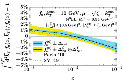
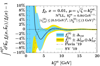
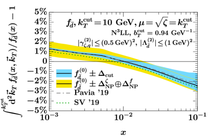
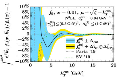

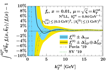
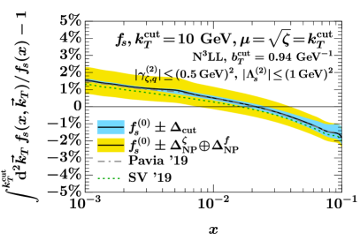
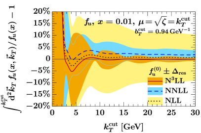
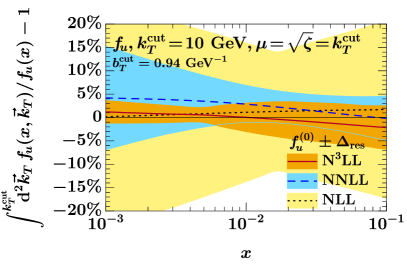

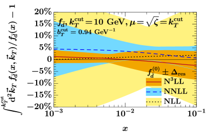
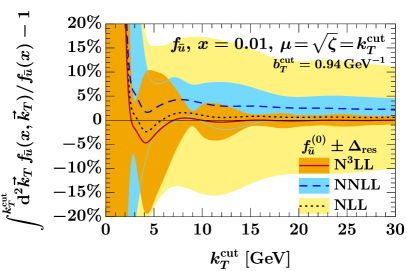

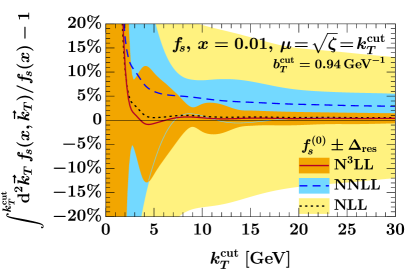
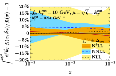
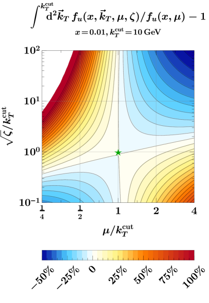


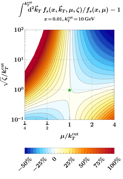
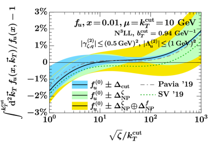
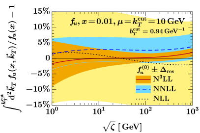

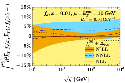
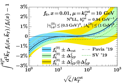

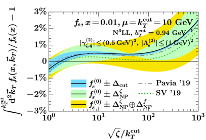
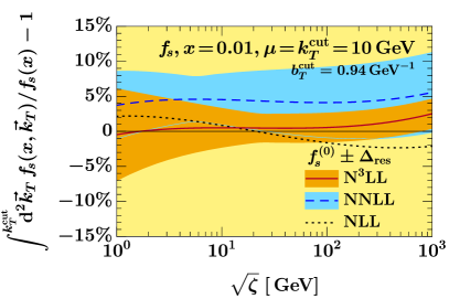
References
- [1] ATLAS collaboration, Measurement of the Transverse Momentum Distribution of Bosons in Collisions at TeV with the ATLAS Detector, Phys. Rev. D 85 (2012) 012005 [1108.6308].
- [2] ATLAS collaboration, Measurement of the boson transverse momentum distribution in collisions at = 7 TeV with the ATLAS detector, JHEP 09 (2014) 145 [1406.3660].
- [3] ATLAS collaboration, Measurement of the transverse momentum and distributions of Drell-Yan lepton pairs in proton-proton collisions at TeV with the ATLAS detector, Eur. Phys. J. C76 (2016) 291 [1512.02192].
- [4] ATLAS collaboration, Measurement of the -boson mass in pp collisions at TeV with the ATLAS detector, Eur. Phys. J. C78 (2018) 110 [1701.07240].
- [5] ATLAS collaboration, Measurement of the Drell-Yan triple-differential cross section in collisions at TeV, JHEP 12 (2017) 059 [1710.05167].
- [6] ATLAS collaboration, Measurement of the transverse momentum distribution of Drell-Yan lepton pairs in proton-proton collisions at TeV with the ATLAS detector, Eur. Phys. J. C 80 (2020) 616 [1912.02844].
- [7] CMS collaboration, Measurement of the Rapidity and Transverse Momentum Distributions of Bosons in Collisions at TeV, Phys. Rev. D 85 (2012) 032002 [1110.4973].
- [8] CMS collaboration, Measurement of the Z boson differential cross section in transverse momentum and rapidity in proton–proton collisions at 8 TeV, Phys. Lett. B 749 (2015) 187 [1504.03511].
- [9] CMS collaboration, Measurement of the transverse momentum spectra of weak vector bosons produced in proton-proton collisions at TeV, JHEP 02 (2017) 096 [1606.05864].
- [10] CMS collaboration, Measurement of differential cross sections in the kinematic angular variable for inclusive Z boson production in pp collisions at 8 TeV, JHEP 03 (2018) 172 [1710.07955].
- [11] CMS collaboration, Measurements of differential Z boson production cross sections in proton-proton collisions at 13 TeV, JHEP 12 (2019) 061 [1909.04133].
- [12] LHCb collaboration, R. Aaij et al., Measurement of the forward Z boson production cross-section in pp collisions at TeV, JHEP 09 (2016) 136 [1607.06495].
- [13] LHCb collaboration, R. Aaij et al., Measurement of the W boson mass, JHEP 01 (2022) 036 [2109.01113].
- [14] A. Accardi et al., Electron Ion Collider: The Next QCD Frontier, Eur. Phys. J. A52 (2016) 268 [1212.1701].
- [15] H. Gao, T. Liu and Z. Zhao, The TMD Program at JLab, PoS DIS2018 (2018) 232.
- [16] T. Liu, TMD program at Jefferson Lab, PoS CD2018 (2019) 036.
- [17] R. Abdul Khalek et al., Science Requirements and Detector Concepts for the Electron-Ion Collider: EIC Yellow Report, 2103.05419.
- [18] J. Collins, Foundations of perturbative QCD, vol. 32. Cambridge University Press, 11, 2013.
- [19] Z.-B. Kang, X. Liu, F. Ringer and H. Xing, The transverse momentum distribution of hadrons within jets, JHEP 11 (2017) 068 [1705.08443].
- [20] Z.-B. Kang, A. Prokudin, F. Ringer and F. Yuan, Collins azimuthal asymmetries of hadron production inside jets, Phys. Lett. B 774 (2017) 635 [1707.00913].
- [21] Y. Makris, D. Neill and V. Vaidya, Probing Transverse-Momentum Dependent Evolution With Groomed Jets, JHEP 07 (2018) 167 [1712.07653].
- [22] D. Gutierrez-Reyes, I. Scimemi, W. J. Waalewijn and L. Zoppi, Transverse momentum dependent distributions with jets, Phys. Rev. Lett. 121 (2018) 162001 [1807.07573].
- [23] D. Gutierrez-Reyes, I. Scimemi, W. J. Waalewijn and L. Zoppi, Transverse momentum dependent distributions in and semi-inclusive deep-inelastic scattering using jets, JHEP 10 (2019) 031 [1904.04259].
- [24] D. Gutierrez-Reyes, Y. Makris, V. Vaidya, I. Scimemi and L. Zoppi, Probing Transverse-Momentum Distributions With Groomed Jets, JHEP 08 (2019) 161 [1907.05896].
- [25] J. C. Collins and D. E. Soper, Back-To-Back Jets: Fourier Transform from B to K-Transverse, Nucl. Phys. B 197 (1982) 446.
- [26] A. Bacchetta, F. Delcarro, C. Pisano, M. Radici and A. Signori, Extraction of partonic transverse momentum distributions from semi-inclusive deep-inelastic scattering, Drell-Yan and Z-boson production, JHEP 06 (2017) 081 [1703.10157].
- [27] I. Scimemi and A. Vladimirov, Systematic analysis of double-scale evolution, JHEP 08 (2018) 003 [1803.11089].
- [28] G. Lustermans, J. K. L. Michel, F. J. Tackmann and W. J. Waalewijn, Joint two-dimensional resummation in and -jettiness at NNLL, JHEP 03 (2019) 124 [1901.03331].
- [29] M. G. Echevarria, A. Idilbi and I. Scimemi, Factorization Theorem For Drell-Yan At Low And Transverse Momentum Distributions On-The-Light-Cone, JHEP 1207 (2012) 002 [1111.4996].
- [30] M. G. Echevarria, A. Idilbi and I. Scimemi, Soft and Collinear Factorization and Transverse Momentum Dependent Parton Distribution Functions, Phys.Lett. B726 (2013) 795 [1211.1947].
- [31] J.-y. Chiu, A. Jain, D. Neill and I. Z. Rothstein, The Rapidity Renormalization Group, Phys. Rev. Lett. 108 (2012) 151601 [1104.0881].
- [32] J.-Y. Chiu, A. Jain, D. Neill and I. Z. Rothstein, A Formalism for the Systematic Treatment of Rapidity Logarithms in Quantum Field Theory, JHEP 1205 (2012) 084 [1202.0814].
- [33] M. A. Ebert, I. W. Stewart and Y. Zhao, Towards Quasi-Transverse Momentum Dependent PDFs Computable on the Lattice, JHEP 09 (2019) 037 [1901.03685].
- [34] D. E. Soper, Partons and Their Transverse Momenta in QCD, Phys. Rev. Lett. 43 (1979) 1847.
- [35] J. C. Collins and D. E. Soper, Back-To-Back Jets in QCD, Nucl. Phys. B193 (1981) 381.
- [36] X.-d. Ji, J.-p. Ma and F. Yuan, QCD factorization for semi-inclusive deep-inelastic scattering at low transverse momentum, Phys. Rev. D71 (2005) 034005 [hep-ph/0404183].
- [37] M. A. Ebert, S. T. Schindler, I. W. Stewart and Y. Zhao, Factorization connecting continuum and lattice TMDs, to appear.
- [38] I. Scimemi and A. Vladimirov, Non-perturbative structure of semi-inclusive deep-inelastic and Drell-Yan scattering at small transverse momentum, JHEP 06 (2020) 137 [1912.06532].
- [39] A. Bacchetta, V. Bertone, C. Bissolotti, G. Bozzi, F. Delcarro, F. Piacenza et al., Transverse-momentum-dependent parton distributions up to N3LL from Drell-Yan data, JHEP 07 (2020) 117 [1912.07550].
- [40] J.-w. Qiu and X.-f. Zhang, Role of the nonperturbative input in QCD resummed Drell-Yan distributions, Phys. Rev. D 63 (2001) 114011 [hep-ph/0012348].
- [41] E. L. Berger and J.-w. Qiu, Differential cross-section for Higgs boson production including all orders soft gluon resummation, Phys. Rev. D 67 (2003) 034026 [hep-ph/0210135].
- [42] CMS collaboration, Measurements of differential Z boson production cross sections in proton-proton collisions at = 13 TeV, JHEP 12 (2019) 061 [1909.04133].
- [43] ATLAS collaboration, Measurement of the transverse momentum distribution of Drell–Yan lepton pairs in proton–proton collisions at TeV with the ATLAS detector, Eur. Phys. J. C 80 (2020) 616 [1912.02844].
- [44] P. Shanahan, M. L. Wagman and Y. Zhao, Nonperturbative renormalization of staple-shaped Wilson line operators in lattice QCD, Phys. Rev. D101 (2020) 074505 [1911.00800].
- [45] P. Shanahan, M. Wagman and Y. Zhao, Collins-Soper kernel for TMD evolution from lattice QCD, Phys. Rev. D102 (2020) 014511 [2003.06063].
- [46] M. Schlemmer, A. Vladimirov, C. Zimmermann, M. Engelhardt and A. Schäfer, Determination of the Collins-Soper Kernel from Lattice QCD, JHEP 08 (2021) 004 [2103.16991].
- [47] Lattice Parton collaboration, Q.-A. Zhang et al., Lattice QCD Calculations of Transverse-Momentum-Dependent Soft Function through Large-Momentum Effective Theory, Phys. Rev. Lett. 125 (2020) 192001 [2005.14572].
- [48] Y. Li et al., Systematic study of transverse-momentum dependent soft function from lattice QCD, 2106.13027.
- [49] P. Shanahan, M. Wagman and Y. Zhao, Lattice QCD calculation of the Collins-Soper kernel from quasi-TMDPDFs, Phys. Rev. D 104 (2021) 114502 [2107.11930].
- [50] R. Boussarie, M. Burkardt, M. Constantinou, W. Detmold, M. Ebert, M. Engelhardt et al., TMD Handbook, work in progress.
- [51] M. G. Echevarria, A. Idilbi and I. Scimemi, Factorization Theorem For Drell-Yan At Low And Transverse Momentum Distributions On-The-Light-Cone, JHEP 07 (2012) 002 [1111.4996].
- [52] J. C. Collins and D. E. Soper, Parton Distribution and Decay Functions, Nucl. Phys. B194 (1982) 445.
- [53] A. Bacchetta and A. Prokudin, Evolution of the helicity and transversity Transverse-Momentum-Dependent parton distributions, Nucl. Phys. B 875 (2013) 536 [1303.2129].
- [54] K. Soni, Asymptotic expansion of the hankel transform with explicit remainder terms, Quarterly of Applied Mathematics 40 (1982) 1.
- [55] E. C. Titchmarsh, Introduction to the theory of Fourier integrals. The Clarendon Press, Oxford, 2nd ed., 1948.
- [56] “NIST Digital Library of Mathematical Functions.” http://dlmf.nist.gov/, Release 1.1.1 of 2021-03-15.
- [57] M. A. Shifman, Quark hadron duality, in 8th International Symposium on Heavy Flavor Physics, vol. 3, (Singapore), pp. 1447–1494, World Scientific, 7, 2000, hep-ph/0009131.
- [58] A. Vladimirov, Pion-induced Drell-Yan processes within TMD factorization, JHEP 10 (2019) 090 [1907.10356].
- [59] J. Collins and T. Rogers, Understanding the large-distance behavior of transverse-momentum-dependent parton densities and the Collins-Soper evolution kernel, Phys. Rev. D 91 (2015) 074020 [1412.3820].
- [60] J. Collins, L. Gamberg, A. Prokudin, T. C. Rogers, N. Sato and B. Wang, Relating Transverse Momentum Dependent and Collinear Factorization Theorems in a Generalized Formalism, Phys. Rev. D 94 (2016) 034014 [1605.00671].
- [61] A. A. Vladimirov, Self-contained definition of the Collins-Soper kernel, Phys. Rev. Lett. 125 (2020) 192002 [2003.02288].
- [62] T. Lübbert, J. Oredsson and M. Stahlhofen, Rapidity renormalized TMD soft and beam functions at two loops, JHEP 03 (2016) 168 [1602.01829].
- [63] Y. Li and H. X. Zhu, Bootstrapping Rapidity Anomalous Dimensions for Transverse-Momentum Resummation, Phys. Rev. Lett. 118 (2017) 022004 [1604.01404].
- [64] A. A. Vladimirov, Correspondence between Soft and Rapidity Anomalous Dimensions, Phys. Rev. Lett. 118 (2017) 062001 [1610.05791].
- [65] V. Moos and A. Vladimirov, Calculation of transverse momentum dependent distributions beyond the leading power, JHEP 12 (2020) 145 [2008.01744].
- [66] M. A. Ebert, J. K. L. Michel, F. J. Tackmann et al., SCETlib: A C++ Package for Numerical Calculations in QCD and Soft-Collinear Effective Theory, DESY-17-099, webpage: http://scetlib.desy.de.
- [67] M. A. Ebert, J. K. L. Michel, I. W. Stewart and F. J. Tackmann, Drell-Yan resummation of fiducial power corrections at N3LL, JHEP 04 (2021) 102 [2006.11382].
- [68] T. Gehrmann, T. Lübbert and L. L. Yang, Transverse parton distribution functions at next-to-next-to-leading order: the quark-to-quark case, Phys. Rev. Lett. 109 (2012) 242003 [1209.0682].
- [69] T. Gehrmann, T. Lübbert and L. L. Yang, Calculation of the transverse parton distribution functions at next-to-next-to-leading order, JHEP 06 (2014) 155 [1403.6451].
- [70] S. Moch, J. A. M. Vermaseren and A. Vogt, The Quark form-factor at higher orders, JHEP 08 (2005) 049 [hep-ph/0507039].
- [71] J. M. Henn, G. P. Korchemsky and B. Mistlberger, The full four-loop cusp anomalous dimension in super Yang-Mills and QCD, JHEP 04 (2020) 018 [1911.10174].
- [72] A. von Manteuffel, E. Panzer and R. M. Schabinger, Analytic four-loop anomalous dimensions in massless QCD from form factors, Phys. Rev. Lett. 124 (2020) 162001 [2002.04617].
- [73] T.-J. Hou et al., New CTEQ global analysis of quantum chromodynamics with high-precision data from the LHC, Phys. Rev. D 103 (2021) 014013 [1912.10053].
- [74] A. Buckley, J. Ferrando, S. Lloyd, K. Nordström, B. Page, M. Rüfenacht et al., LHAPDF6: parton density access in the LHC precision era, Eur. Phys. J. C 75 (2015) 132 [1412.7420].
- [75] T. van Ritbergen, J. A. M. Vermaseren and S. A. Larin, The Four loop beta function in quantum chromodynamics, Phys. Lett. B400 (1997) 379 [hep-ph/9701390].
- [76] M. Czakon, The Four-loop QCD beta-function and anomalous dimensions, Nucl. Phys. B710 (2005) 485 [hep-ph/0411261].
- [77] C. W. Groetsch, Lanczos’ generalized derivative, The American Mathematical Monthly 105 (1998) 320.
- [78] S. Rangarajan and S. P. Purushothaman, Lanczos’ generalized derivative for higher orders, Journal of Computational and Applied Mathematics 177 (2005) 461.
- [79] H. Takahasi and M. Mori, Double exponential formulas for numerical integration, Pub. RIMS 9 (1974) 721.
- [80] T. Ooura, A continuous euler transformation and its application to the fourier transform of a slowly decaying function, J. Comput. Appl. Math. 130 (2001) 259.
- [81] T. Ooura, Study on numerical integration of Fourier type integrals, Ph.D. thesis, University of Tokyo, 1997.
- [82] I. Scimemi and A. Vladimirov, Analysis of vector boson production within TMD factorization, Eur. Phys. J. C 78 (2018) 89 [1706.01473].
- [83] “NangaParbat landing page.” https://github.com/MapCollaboration/NangaParbat.
- [84] “NangaParbat report on the PV19x_N3LL fit.” https://vbertone.github.io/NangaParbat/results/PV19/N3LL/index.html.
- [85] Y. Li, D. Neill and H. X. Zhu, An exponential regulator for rapidity divergences, Nucl. Phys. B 960 (2020) 115193 [1604.00392].
- [86] J. C. Collins and D. E. Soper, Angular Distribution of Dileptons in High-Energy Hadron Collisions, Phys. Rev. D16 (1977) 2219.
- [87] J. C. Collins, D. E. Soper and G. F. Sterman, Transverse Momentum Distribution in Drell-Yan Pair and W and Z Boson Production, Nucl. Phys. B250 (1985) 199.
- [88] M.-x. Luo, T.-Z. Yang, H. X. Zhu and Y. J. Zhu, Quark Transverse Parton Distribution at the Next-to-Next-to-Next-to-Leading Order, Phys. Rev. Lett. 124 (2020) 092001 [1912.05778].
- [89] M. A. Ebert, B. Mistlberger and G. Vita, TMD Fragmentation Functions at N3LO, JHEP 07 (2021) 121 [2012.07853].
- [90] M.-x. Luo, T.-Z. Yang, H. X. Zhu and Y. J. Zhu, Unpolarized quark and gluon TMD PDFs and FFs at N3LO, JHEP 06 (2021) 115 [2012.03256].
- [91] S. Camarda, L. Cieri and G. Ferrera, Drell–Yan lepton-pair production: qT resummation at N3LL accuracy and fiducial cross sections at N3LO, Phys. Rev. D 104 (2021) L111503 [2103.04974].
- [92] E. Re, L. Rottoli and P. Torrielli, Fiducial Higgs and Drell-Yan distributions at N3LL′+NNLO with RadISH, 2104.07509.
- [93] W.-L. Ju and M. Schönherr, The qT and spectra in W and Z production at the LHC at N3LL’+N2LO, JHEP 10 (2021) 088 [2106.11260].
- [94] G. Billis, M. A. Ebert, J. K. L. Michel and F. J. Tackmann, Drell-Yan spectrum at N3LL′ with SCETlib, to appear.
- [95] L. Cieri, G. Ferrera and G. F. R. Sborlini, Combining QED and QCD transverse-momentum resummation for Z boson production at hadron colliders, JHEP 08 (2018) 165 [1805.11948].
- [96] A. Bacchetta and M. G. Echevarria, QCDQED evolution of TMDs, Phys. Lett. B 788 (2019) 280 [1810.02297].
- [97] G. Billis, F. J. Tackmann and J. Talbert, Higher-Order Sudakov Resummation in Coupled Gauge Theories, JHEP 03 (2020) 182 [1907.02971].
- [98] P. Pietrulewicz, D. Samitz, A. Spiering and F. J. Tackmann, Factorization and Resummation for Massive Quark Effects in Exclusive Drell-Yan, JHEP 08 (2017) 114 [1703.09702].
- [99] S. Mantry and F. Petriello, Factorization and Resummation of Higgs Boson Differential Distributions in Soft-Collinear Effective Theory, Phys. Rev. D 81 (2010) 093007 [0911.4135].
- [100] M. Burkardt, Sivers mechanism for gluons, Phys. Rev. D 69 (2004) 091501 [hep-ph/0402014].
- [101] K. Soni, Exact error terms in the asymptotic expansion of a class of integral transforms i. oscillatory kernels, SIAM journal on mathematical analysis 11 (1980) 828.
- [102] R. Wong, Error bounds for asymptotic expansions of integrals, SIAM review 22 (1980) 401.