Online, Informative MCMC Thinning with Kernelized Stein Discrepancy

Abstract

A fundamental challenge in Bayesian inference is efficient representation of a target distribution. Many non-parametric approaches do so by sampling a large number of points using variants of Markov Chain Monte Carlo (MCMC). We propose an MCMC variant that retains only those posterior samples which exceed a KSD threshold, which we call KSD Thinning. We establish the convergence and complexity tradeoffs for several settings of KSD Thinning as a function of the KSD threshold parameter, sample size, and other problem parameters. Finally, we provide experimental comparisons against other online nonparametric Bayesian methods that generate low-complexity posterior representations, and observe superior consistency/complexity tradeoffs. Our attached code will be made public.

1 Introduction

Uncertainty quantification aids automated decision-making by permitting risk evaluation and expert deferral in applications such as medical imaging and autonomous driving. Nonparametric Bayesian inference methods such as Markov Chain Monte Carlo (MCMC) are the gold standard in uncertainty estimation problems, but sample complexity is a major bottleneck in their practical application. A major limitation of MCMC is that the samples generated by a transition kernel are correlated, which can lead to redundancy in the constructed estimate.

In uncertainty quantification each retained sample corresponds to one expensive forward simulation (Constantine et al., 2016; Peherstorfer et al., 2018; Martin et al., 2012) and in machine learning each retained sample requires the storage and inference costs of a expensive model such as a neural network (Neal, 2012; Lakshminarayanan et al., 2016). Therefore balancing representation quality and representational complexity is an important tradeoff. In standard MCMC, to ensure statistical consistency, the representational complexity approaches infinity. Classically, to deal with the redundancy issue, one may employ online or post-hoc “thinning,” which discards all but a random subset of MCMC samples (Raftery & Lewis, 1996; Link & Eaton, 2012). More recently this task is sometimes called “quantizing” a posterior distribution (Riabiz et al., 2020), especially when the work studies Bayesian cubature (Teymur et al., 2020). Existing approaches generate a large set of samples (usually via MCMC) and then “thin” the sample set. Doing so may require storing a large number of samples before the final post-processing stage (Riabiz et al., 2020; Teymur et al., 2020) and does not allow the sampler to target a compressed representation during the MCMC iterations. Traditional online thinning is done without any goodness-of-fit metric on the samples, which may ignore gradient information generated by modern stochastic gradient MCMC methods (Welling & Teh, 2011; Ma et al., 2015).

To select samples to retain during thinning, one may compute metrics between the empirical measure and the unknown target $\mathbb{P}$. However, in a Bayesian inference context, many popular integral probability metrics (IPM) are not computable. The kernelized Stein discrepancy (KSD) addresses this by employing the score function of the target combined with reproducing kernel Hilbert Space (RKHS) distributional embeddings to define statistics that track the discrepancy between distributions in a computationally feasible manner (Berlinet & Thomas-Agnan, 2011; Sriperumbudur et al., 2010; Stein, 1972; Liu et al., 2016).

1.1 Related Work

Several MCMC thinning procedures have been developed based upon RKHS embedding: Offline methods such as Stein Thinning and MMD thinning (Riabiz et al., 2020; Teymur et al., 2020; Dwivedi & Mackey, 2021) take a full chain $\mathbf{S}$ of MCMC samples as input and iteratively build a subset $\mathbf{D}$ by greedy KSD/MMD minimization. The online method Stein Point MCMC (SPMCMC) (Chen et al., 2019a) selects the optimal sample from a batch of $m$ samples during MCMC sampling: at each step it adds the best of $m$ points to a $\mathbf{D}$. Doing so mitigates both the aforementioned redundancy and representational complexity issues; however (Chen et al., 2019a) only append new points to the existing empirical measure estimates, which may still retain too many redundant points. Another online approach maintains a fixed-size reservoir of samples, but the reservoir size is pre-fixed (Paige et al., 2016).

A similar line of research in Gaussian Processes (Williams & Rasmussen, 2006) and kernel regression (Hofmann et al., 2008) reduces the complexity of a nonparametric distributional representation through offline point selection rules such as Nyström sampling (Williams & Seeger, 2001), greedy forward selection (Seeger et al., 2003; Wang et al., 2012), or inducing inputs (Snelson & Ghahramani, 2005). In Gaussian processes fixing the approximation error instead of the representational complexity, and allowing both constructive/destructive operations in the dictionary selection, yields improved distributional estimates when employing online sample processing (Koppel et al., 2017, 2020).

Most similar to our work is a variant of Stein Point MCMC proposed in (Chen et al., 2019a)[Appendix A.6.5] which develops a non-adaptive add/drop criterion where a pre-fixed number of points are dropped at each stage and the dictionary size grows linearly with the time step. By contrast, our work develops a flexible and adaptive scheme that automatically determines the number of points to drop and the dictionary size grows sub-linearly with the time step.

1.2 Contributions

Method	Online	Informative	Discard Past Samples	Model Order Growth
MCMC Thinning	✓	✗	✗	$n$
Stein Thinning (Riabiz et al., 2020)	✗	✓	✓	NA
SPMCMC (Chen et al., 2019a)	✓	✓	✗	$n$
This work	✓	✓	✓	$o\left(\sqrt{n\log(n)}\right)$

Table 1: Methods for Generating Compressed Non-Parametric Representations

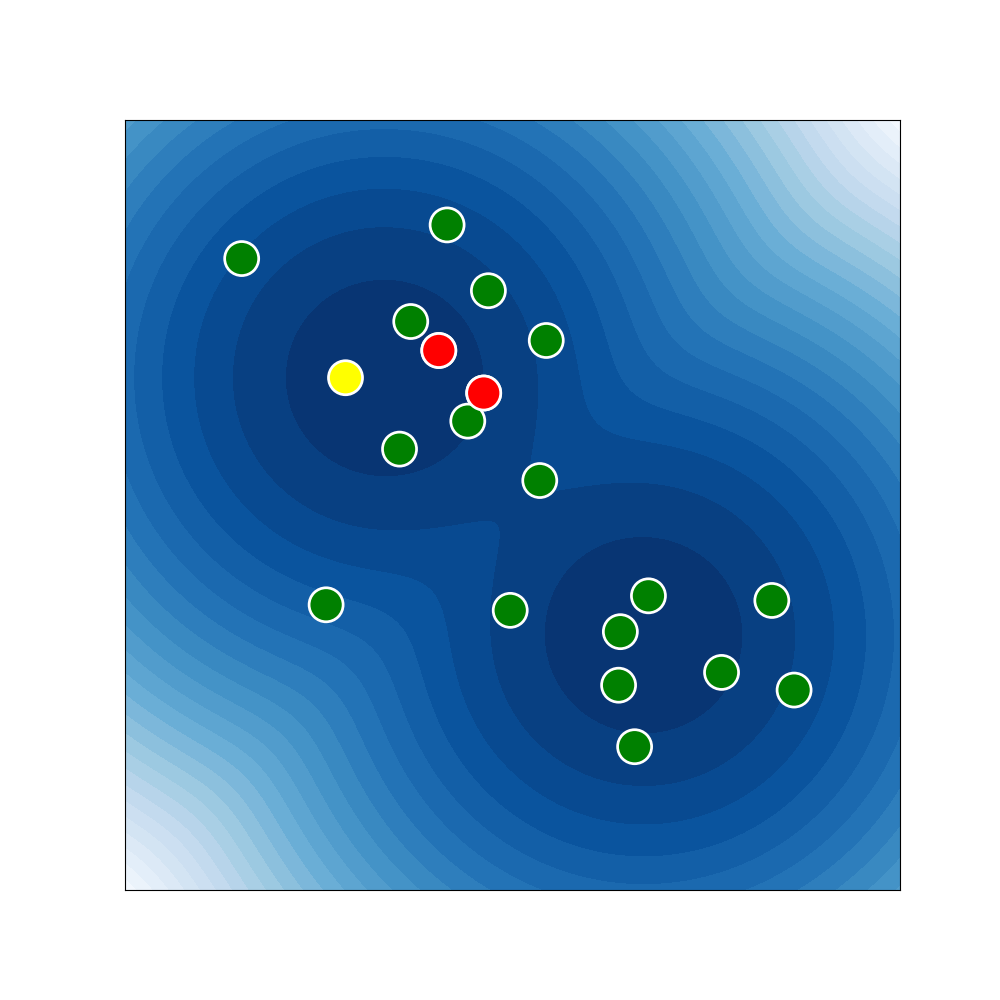
Figure 1: Current dictionary $\mathbf{D}_{t-1}$ in green. New sample $\mathbf{x}_{t}$ added in yellow to form $\tilde{\mathbf{D}}_{t}$. Then redundant red samples are thinned.

We propose a method that generates a compressed representation by flexible and online thinning of a stream of MCMC samples. Our method specifies a KSD budget parameter which determines both the transient dictionary complexity and asymptotic bias of the inference by allowing both constructive and destructive point selection during sampling, rather than after the fact. In contrast to existing online approaches that require linear growth in the size of the active set we require only $o\left(\sqrt{n\log(n)}\right)$ growth to ensure convergence through a novel memory-reduction routine we call Kernelized Stein Discrepancy Thinning (KSDT). We compare our approach and several others in Table 1. Our method, described at a high level in Figure 1, enables sample-efficient Bayesian learning by directly targeting compressed representations during the sampling process. We make the following specific contributions:

• We introduce the first online thinning algorithm that can provide informative removal of past MCMC samples during the sampling process. Our algorithm permits a flexible tradeoff between model order growth, thinning budget, and posterior consistency.

• We prove in Theorem 1 that our thinning method can be applied to existing SOTA MCMC algorithms with no change in asymptotic convergence rate when the thinning budget asymptotically decays to $0$. In Corollary 1 we provide the KSD neighborhood of convergence when the thinning budget is fixed.

• We test our method on two MCMC problems from the biological sciences and two Bayesian Neural Network problems and demonstrate that our thinning algorithm can reduce the number of retained samples but retain or improve baseline sampler performance.

2 Online KSD Thinning

Given a sequence of points $\mathbf{S}=\{\mathbf{x}_{i}\}_{i=1}^{N}$ drawn from an unknown probability measure $\mathbb{P}$ with $\mathbf{x}_{i}\in\mathcal{X}\subset\mathbb{R}^{d}$, our goal is to infer an approximate empirical measure $q_{\mathbf{D}}=\hat{\mathbb{P}}$. Here $q_{\mathbf{D}}$ is a particle representation with a sparse dictionary $\mathbf{D}\subsetneq\mathbf{S}$, i.e., $|\mathbf{D}|\ll N$, where $N\leq\infty$ is the potentially infinite sample size. Specifically, the approximate density associated with $\mathbf{D}$ takes the form

$$q_{\mathbf{D}}(\cdot)=\frac{1}{|\mathbf{D}|}\sum_{\mathbf{x}_{i}\in\mathbf{D}}\delta_{\mathbf{x}_{i}}(\cdot),$$ (1)

where $\delta_{\mathbf{x}_{i}}$ denotes the Dirac delta which is $1$ if its argument is equal to $\mathbf{x}_{i}$, and $0$ otherwise.

We assume that the measure $\mathbb{P}$ admits a density $p$ which can only be evaluated up to an unknown normalization constant. That is, $p=\tilde{p}/Z$ with $\tilde{p}$ as the unnormalized density and $Z>0$ as the normalization constant. We assume that the unnormalized density $\tilde{p}$ and its score function $\nabla\log\tilde{p}$ may be evaluated in a computationally affordable manner. This set of assumptions is standard in many Bayesian inference problems that arise in machine learning and uncertainty quantification (Welling & Teh, 2011; Chen et al., 2019a; Constantine et al., 2016; Peherstorfer et al., 2018).

Our goal is construct $\mathbf{D}$ from the stream of samples $\mathbf{S}$ by determining which points to retain from $\mathbf{S}$ and discard from $\mathbf{D}$. The empirical distribution $q_{\mathbf{D}}$ can then be used to approximate integrals of the form

$$\int_{\mathcal{X}}f(\mathbf{x})p(\mathbf{x})d\mathbf{x}\approx\frac{1}{|\mathbf{D}|}\sum_{\mathbf{x}_{i}\in\mathbf{D}}f(\mathbf{x}_{i}).$$ (2)

2.1 Kernelized Stein Discrepancy

Informative thinning requires a goodness-of-fit metric to distinguish between “good” samples and “bad” samples. In general, evaluation of metrics between the empirical estimate $q_{\mathbf{D}}$ and the target $p$ is intractable. The powerful combination of Stein’s method (Stein, 1972) and Reproducing Kernel Hilbert Spaces (Berlinet & Thomas-Agnan, 2011; Sriperumbudur et al., 2010) permits one to evaluate discrepancies between $q_{\mathbf{D}}$ and $p$ in closed form (Liu et al., 2016). Let $k$ be a base kernel, for example the inverse multi-quadratic (IMQ) kernel

$$k(\mathbf{x},\mathbf{y})=\left(1+\|\mathbf{x}-\mathbf{y}\|_{2}^{2}\right)^{-0.5}$$ (3)

or the Radial Basis Function (RBF) kernel

$$k(\mathbf{x},\mathbf{y})=\exp\left(-\|\mathbf{x}-\mathbf{y}\|_{2}^{2}/2h\right).$$ (4)

Next define the Stein kernel

$$\begin{split}k_{0}(\mathbf{x},\mathbf{y})=&\nabla_{\mathbf{x}}\log p(\mathbf{x})^{T}\nabla_{\mathbf{y}}\log p(\mathbf{y})k(\mathbf{x},\mathbf{y})\\ &+\nabla_{\mathbf{y}}\log p(\mathbf{y})^{T}\nabla_{\mathbf{x}}k(\mathbf{x},\mathbf{y})\\ &+\nabla_{\mathbf{x}}\log p(\mathbf{x})^{T}\nabla_{\mathbf{y}}k(\mathbf{x},\mathbf{y})+\sum_{i=1}^{d}\frac{\partial^{2}k(\mathbf{x},\mathbf{y})}{\partial\mathbf{x}_{i}\partial\mathbf{y}_{i}}\;,\end{split}$$ (5)

where $p$ is a fixed target density, $d$ is the dimension of each particle $\mathbf{x},\mathbf{y}\in\mathcal{X}$ and the score function $\nabla_{\mathbf{x}}\log p(\mathbf{x})$ can be estimated without knowledge of the normalizing constants $Z$. Stein’s method in this context specifies a constructed RKHS $\mathcal{K}_{0}$ with Stein kernel $k_{0}$ (5) in turn constructed from the base kernel $k$. Then the kernelized Stein discrepancy (KSD) of an empirical measure $q_{\mathbf{D}}$ with respect to a target density $p$ is the RKHS norm in $\mathcal{K}_{0}$ given by

$${\rm KSD}(q_{\mathbf{D}})=\sqrt{\frac{1}{n^{2}}\sum_{\mathbf{x}_{i},\mathbf{x}_{j}\in\mathbf{D}}k_{0}(\mathbf{x}_{i},\mathbf{x}_{j})}.$$ (6)

For simplicity our notation suppresses the dependence on the target density $p$ and the RKHS $\mathcal{K}$.

2.2 Online Thinning - Outer Loop

0:  Target density $p$, initial dictionary $\mathbf{D}_{0}$, point sequence $\mathbf{S}=\{\mathbf{x}_{i}\}_{i=1}^{\infty}$, budget sequence $\{\epsilon_{t}\}_{t=1}^{\infty}$, minimum sample size function $f$.

  for $t$ in $[1,2,3,\dots]$ do

     Receive new sample $\mathbf{x}_{t}$ from $\mathbf{S}$

     Add sample $\mathbf{x}_{t}$ to dictionary: $\tilde{\mathbf{D}}_{t}=\mathbf{D}_{t-1}\cup\{\mathbf{x}_{t}\}$

     Thin via Algorithm 2: $\mathbf{D}_{t}=\texttt{ KSDT}(p,\tilde{\mathbf{D}}_{t},\epsilon_{t},f(t))$

  end for

Algorithm 1 Online KSD Thinning (KSDT)

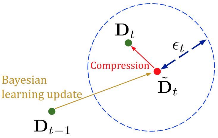
Figure 2: A geometric view of online KSD thinning (Algorithm 1). We update $\mathbf{D}_{t-1}$, fix a KSD $\epsilon$-neighborhood, and greedily remove points until we hit the boundary of this neighborhood. By tuning the compression-induced error to the information contained in the update direction, i.e., the red arrow representing Eq. (7), we obtain the green dot $\mathbf{D}_{t}$, which is the update output by Algorithm 2.

In Algorithm 1 we propose an online thinning algorithm that can generate compressed representations of a measure $\mathbb{P}$ with access only to a stream of samples $\mathbf{S}$, the unnormalized density $\tilde{p}$, and the score function $\nabla\log\tilde{p}$. Our sampler performs informative thinning in a flexible online fashion by discarding points that do not make a sufficient contribution to minimizing the KSD objective ${\rm KSD}(q_{\mathbf{D}_{t}})$ where $\mathbf{D}_{t}$ is the thinned dictionary produced by step $t$ of our algorithm.

At each time step $t$ we take previous dictionary $\mathbf{D}_{t-1}$ and add a new sample $\mathbf{x}_{t}$ from our MCMC chain, which results in the expanded auxiliary dictionary:

$$\tilde{\mathbf{D}}_{t}=\mathbf{D}_{t-1}\cup\{\mathbf{x}_{t}\}\;,$$ (7)

which we compress via a destructive inner loop. This outer loop pseudo-code is given in Algorithm 1. If the sample stream $\mathbf{S}$ is generated by an MCMC method and we skip the destructive thinning inner loop then $\mathbf{D}_{t}=\tilde{\mathbf{D}}_{t}$ and the update rule exactly matches standard MCMC.

At each step the thinning budget schedule $\epsilon_{t}$ controls the compression/fidelity tradeoff of the thinned approximation. The minimum dictionary size function $f(t)$ must satisfy the relationship $f(t)=\Omega\left(\sqrt{t\log(t)}\right)$ to preserve the consistency our algorithm. However, if one tolerates non-vanishing asymptotic bias, then $f(t)$ may be set to a small constant $\epsilon_{t}=\epsilon$. We discuss practical selection of $\epsilon$ and the resultant dictionary $\mathbf{D}$ in the following section. Our approach differs from the related work of (Chen et al., 2019a) in that we thin the entire dictionary at each step. In contrast, no prior samples are thinned in the Stein Point MCMC algorithm presented by (Chen et al., 2019a). By thinning the entire dictionary we can remove previously sampled points that are inessential for ensuring the representation is consistent. A major advantage of this approach is that our online thinning algorithm can automatically determine the number of points required based on the complexity of the target measure $\mathbb{P}$. We demonstrate this in Section 4.4.

2.3 Online Thinning - Inner Loop

0:  Target density $p$, empirical measure dictionary $\mathbf{D}$, budget $\epsilon$, minimum sample number $S$

  Compute reference KSD: $M={\rm KSD}(q_{\mathbf{D}})$

  while ${\rm KSD}(q_{\mathbf{D}})^{2}<M^{2}+\epsilon$ and $|\mathbf{D}|>S$ do

     Compute least influential point $\mathbf{x}_{j}$ as in (9)

     if ${\rm KSD}(q_{\mathbf{D}\setminus\{\mathbf{x}_{j}\}})^{2}<M^{2}+\epsilon$ then

        Remove least influential point, set $\mathbf{D}=\mathbf{D}\setminus\{\mathbf{x}_{j}\}$

     else

        Break loop

     end if

  end while

return thinned dictionary $\mathbf{D}$ satisfying ${\rm KSD}(q_{\mathbf{D}})^{2}<M^{2}+\epsilon$

Algorithm 2 Destructive KSD Thinning

The inner loop performs destructive thinning on the auxiliary dictionary $\tilde{\mathbf{D}}_{t}$ based on a maximum KSD thinning budget $\epsilon_{t}$ and a minimum dictionary size $f(t)$.

Given an intermediate dictionary $\tilde{\mathbf{D}}_{t}$ our goal is to return a compressed representation $\mathbf{D}_{t}\subset{\tilde{\mathbf{D}}_{t}}$ that satisfies

$${\rm KSD}(q_{\mathbf{D}_{t}})^{2}<{\rm KSD}(q_{\tilde{\mathbf{D}}_{t}})^{2}+\epsilon.$$ (8)

The compressed dictionary $\mathbf{D}_{t}$ must be $\epsilon$-close in squared KSD to the uncompressed intermediate dictionary $\tilde{\mathbf{D}}_{t}$. In this section we determine how to build $\mathbf{D}_{t}$.

Related work by (Riabiz et al., 2020; Teymur et al., 2020) present constructive greedy approaches to subset selection during post-hoc thinning. The challenge with online constructive approaches is time complexity, as the inner loop requires $|\tilde{\mathbf{D}}_{t}|$ point selections in the worst case (no points are thinned). We expect that few points will be thinned at each step and so we follow a destructive approach that requires only $|\mathbf{D}_{t}|-|\tilde{\mathbf{D}}_{t}|$ point selections per step. In practice, only 0-2 points are thinned at each step and so $|\mathbf{D}_{t}|-|\tilde{\mathbf{D}}_{t}|\in\{0,1,2\}$ while $|\mathbf{D}_{t}|$ ranges from 10-1000.

Our destructive approach iteratively removes points by selecting the “least influential” point in $\mathbf{D}_{t}$

$$\mathbf{x}_{j}=\text{argmin}_{\mathbf{x}\in\mathbf{D}_{t}}{\rm KSD}(q_{\mathbf{D}_{t}\setminus\{\mathbf{x}\}})$$ (9)

If removing the least influential point would violate the KSD criterion in (8) we do not thin the point and we break the thinning loop. If removing the least influential point does not violate the KSD criterion we update $\mathbf{D}_{t}\leftarrow\mathbf{D}_{t}\setminus\{\mathbf{x}_{j}\}$ and repeat the thinning procedure. The inner loop pseudo-code is given in Algorithm 2 and visualized in Figure 1.

Thinning a single point in this manner every $k$ steps was suggested by (Chen et al., 2019a) in Appendix A.6.5 of their work. The main difference between their work and ours is flexibility: they thin a fixed number of points and do not use a KSD-aware thinning criterion (our budget parameter $\epsilon_{t}$) and so “good” points may be unnecessarily removed or too few “bad” points may be removed. Their work does not present convergence guarantees for this thinning strategy. The worst-case per-step time complexity of our method is $\mathcal{O}\left(t\right)$ which matches (Chen et al., 2019a) (see Appendix 8).

2.4 Sample Stream Filtering Requirement

In addition to our practical goal of informative online thinning, we aim to provide an algorithm with provable convergence. We will thin samples, potentially incurring a KSD increase $\epsilon_{t}$ at each step, we require that our sample stream $\mathbf{S}$ already converges in KSD. Therefore we use the SPMCMC approach of (Chen et al., 2019a) to generate a sample stream $\mathbf{S}$ that provably and rapidly converges in KSD.

SPMCMC Update Rule: Let $\mathbf{D}_{t-1}$ be the current dictionary and $\mathbf{y}_{t,0}$ be the current point. To construct $\tilde{\mathbf{D}}_{t}$ we initialize an MCMC chain at $\mathbf{y}_{t,0}$, generate $m$ MCMC samples $\mathcal{Y}_{t}=\{\mathbf{y}_{t,l}\}_{l=1}^{m}$, and append the KSD-optimal point in $\mathcal{Y}_{t}$ to $\mathbf{D}_{t-1}$:

$$\begin{split}\mathbf{x}_{t}&=\operatorname*{arg\,min}_{\mathbf{y}\in\mathcal{Y}_{t}}{\rm KSD}(\mathbf{D}_{t-1}\cup\{\mathbf{y}\}).\\ \tilde{\mathbf{D}}_{t}&=\mathbf{D}_{t-1}\cup\{\mathbf{x}_{t}\}.\end{split}$$ (10)

In Section 4 we provide empirical evidence that our method is suitable for non-SPMCMC samplers (eg. MALA, RWM).

3 Convergence

Method	Per-step bound	Per-step dictionary size	Thinning
SPMCMC (Chen et al., 2019a)	$\log(n)/n$	$n$	✗
Ours	$n\log(n)/f(n)^{2}$	$f(n)=\Omega\left(\sqrt{n\log(n)}\right)$	✓

Table 2: Quantitive Comparison with SPMCMC. Our proposed approach offers a complexity/consistency tradeoff based on the model order growth $f$ and enables online thinning. When $f(n)\propto n$ our approach achieves the SPMCMC convergence rate but enables thinning.

This section provides convergence guarantees for our proposed KSD-Thinning method (Algorithm 1) under several settings. We consider two sample generation mechanisms: i.i.d. sampling and MCMC sampling, and two settings for the sequence of budget parameters $\{\epsilon_{t}\}$: decaying budget ($\epsilon_{t}\rightarrow 0)$ and fixed budget ($\epsilon_{t}=\epsilon$). The decaying budget setting is most applicable when one desires exact posterior consistency in infinite time, whereas fixed budgets are useful when a specified limiting error tolerance is sufficient. In both decaying and fixed budget settings we prove that:

• Our KSD-Thinning algorithm maintains the same asymptotic KSD convergence rate of the baseline sampler, but gains the ability to thin past samples.

• Our algorithm permits a complexity/consistency trade-off that enables higher particle reduction in exchange for the cost of a slower asymptotic convergence rate.

The convergence guarantees and complexity/consistency trade-offs of the two thinning budget settings are provided in Theorem 1 and Corollary 1, respectively. The most relevant comparison to our work is (Chen et al., 2019a) which achieves an $\mathcal{O}(\log(n)/n)$ rate of KSD convergence. Our main result in Theorem 1 differs from the results of (Chen et al., 2019a) in two respects. If we maintain the same asymptotic convergence rate, we can also thin previous samples. Second, our analysis enables the user to trade off between sublinear $\sqrt{n\log(n)}$ growth of $|\mathbf{D}_{t}|$ instead of the linear growth in $|\mathbf{D}_{t}|$ required by (Chen et al., 2019a) at the cost of a slower asymptotic convergence rate. The main technical novelty of our proof is the decomposition of our per-step bound into two terms: the sampling error term from (Chen et al., 2019a) and a thinning error term introduced by Algorithm 2. We defer proofs to Appendix 6.

3.1 Preliminaries

Before we present our main result we introduce two new definitions to impose standard requirements from (Gorham & Mackey, 2017; Chen et al., 2019a) on the Metropolis-Adjusted Langevin Algorithm (MALA) sampler and the distribution $p$. Informally, we require that that target density does not possess a heavy tail (distantly dissipative) and that accepted proposals have low norm (inwardly convergent). These conditions hold for the MALA sampler targeting standard smooth densities.

Definition 1

A density $p$ with lipschitz score function $\nabla\log\tilde{p}$ is distantly dissipative if

$$\begin{split}\liminf_{r\rightarrow 0}\inf_{\|\mathbf{x}-\mathbf{y}\|\leq r}\left\{\frac{\langle\nabla\log\tilde{p}(\mathbf{x})-\nabla\log\tilde{p}(\mathbf{y}),\mathbf{x}-\mathbf{y}\rangle}{\|\mathbf{x}-\mathbf{y}\|_{2}^{2}}\right\}>0.\\ \end{split}$$ (11)

Any density that is strongly log-concave outside of a compact set is distantly dissipative, and a common example is a Gaussian mixture (Korba et al., 2020).

Definition 2

Let $t(\mathbf{x},\mathbf{y})$ denote the MALA transition kernel, and $\alpha(\mathbf{x},\mathbf{y})$ denote the probabilty of accepting proposal $\mathbf{y}$ given current state $\mathbf{x}$. Let $\mathcal{A}(\mathbf{x})=\{\mathbf{y}\in\mathcal{X}|\alpha(\mathbf{x},\mathbf{y})=1\}$ and $\mathcal{I}(\mathbf{x})=\{\mathbf{y}|\|\mathbf{y}\|_{2}\leq\|\mathbf{x}\|_{2}\}$. A chain generated by the Metropolis-Adjusted Langevin algorithm is inwardly convergent if

$$\lim_{\|\mathbf{x}\|_{2}\rightarrow\infty}\int_{\mathcal{A}(\mathbf{x})\Delta\mathcal{I}(\mathbf{x})}t(\mathbf{x},\mathbf{y})d\mathbf{y}=0$$ (12)

where $\mathcal{A}(\mathbf{x})\Delta\mathcal{I}(\mathbf{x})=\left(\mathcal{A}(\mathbf{x})\cup\mathcal{I}(\mathbf{x})\right)\setminus\left(\mathcal{A}(\mathbf{x})\cap\mathcal{I}(\mathbf{x})\right)$ is the symmetric difference.

In the context of a Gaussian distribution, inward convergence states that when the norm of the current state is large accepted MCMC proposals tend towards the mean. This condition is satisfied in practice by balancing the MALA step size with the norm of the score function. For a thorough discussion see (Roberts & Tweedie, 1996).

3.2 Results

To achieve convergence we require that the model order $|\mathbf{D}_{i}|$ is lower bounded by a monotone increasing function $f(i)=\Omega\left(\sqrt{i\log(i)}\right)$. This lower bound on model order growth controls the convergence rate and influences the sequence of maximum possible thinning budgets $\{\epsilon_{i}\}_{i=1}^{\infty}$.

Theorem 1 (Decaying Thinning Budget)

Assume that the kernel $k_{0}$ satisfies $\mathbb{E}_{\mathbf{y}\sim P}\left[e^{\gamma k_{0}(\mathbf{y},\mathbf{y})}\right]=b<\infty$, dictionary sizes are lower bounded as $|\mathbf{D}_{i}|\geq Cf(i)$ where $f(i)=\Omega\left(\sqrt{i\log(i)}\right)$ and specify the compression budget $\epsilon_{i}=\log(i)/f(i)^{2}$. In either of the following two cases

• Case 1: Candidate samples $\{\mathbf{y}_{i,l}\}^{m_{i}}_{l=1}$ are drawn i.i.d from the target density $p$.

• Case 2: Candidate samples $\{\mathbf{y}_{i,l}\}^{m_{i}}_{l=1}$ are generated by MALA and MALA is inwardly convergent for the distantly dissipative target density $p$.

iterate $\mathbf{D}_{n}={\texttt{KSDT}}(\mathbf{D}_{n-1}\cup\{\mathbf{x}_{n}\},\epsilon_{n})$ of Alg. 1 satisfies

$$\mathbb{E}\left[{\rm KSD}(q_{\mathbf{D}_{n}})^{2}\right]\leq C\frac{n\log(n)}{f(n)^{2}}.$$ (13)

This result illustrates how both the thinning budget $\epsilon_{i}$ and the convergence rate depend on the model order growth $f$. A faster convergence rate requires larger $f$, and therefore both faster model order growth and a smaller thinning budget. Our result introduces a trade off between consistency (quality of representation) and complexity (number of particles retained). If we require that the dictionary size grows linearly with $f(i)\propto i$ then we recover the same $\mathcal{O}(\log(n)/n)$ asymptotic convergence rate of Theorem 1 of (Chen et al., 2019a) but gain the ability to thin past samples in the dictionary. If we choose $f$ that grows at a slower rate then the sequence ${\epsilon_{i}}$ can decay at a slower rate so we can employ more aggressive thinning and achieve a lower-complexity representation at the cost of slower convergence. In practice we found that $\epsilon=0$ is a simple choice of thinning budget with good empirical performance. When $\epsilon=0$ thinning does not increase the KSD. Therefore the required decrease in thinning budget $\epsilon$ as $f$ grows is not a concern.

An important practical case is when we desire a fixed error representation of the density $p$. We set a fixed KSD convergence radius and then determine a constant thinning budget and the required number of steps of Algorithm 1 to achieve a representation of $p$ with KSD error $\Delta$.

Corollary 1 (Constant Thinning Budget)

Fix target KSD convergence radius $\Delta$, assume the same conditions as Theorem 1, and assume that $f(i)\propto\sqrt{i^{1+\alpha}\log(i)}$. With constant thinning budget $\epsilon=\mathcal{O}\left(\Delta^{1+\frac{1}{\alpha}}\right)$, after $n=\mathcal{O}\left(\Delta^{-\frac{1}{\alpha}}\right)$ steps the iterate $\mathbf{D}_{n}$ produced by Algorithm 1 satisfies

$$\mathbb{E}\left[{\rm KSD}\left(q_{\mathbf{D}_{n}}\right)^{2}\right]\leq C\Delta$$ (14)

for generic constant $C$. Equivalently, if we fix a constant thinning budget $\epsilon$, after $n=\mathcal{O}\left(\epsilon^{-\frac{2}{\alpha+1}}\right)$ steps we have

$$\mathbb{E}\left[{\rm KSD}\left(q_{\mathbf{D}_{n}}\right)^{2}\right]\leq C\epsilon^{\frac{2}{1+\frac{1}{\alpha}}}$$ (15)

To our knowledge, this is the first result that specifies the number of MCMC steps required to reach a fixed-error KSD neighborhood of the target density. As in Theorem 1 our result demonstrates a trade-off between the model order growth and convergence rate. In Theorem 1 we did not impose a parametric form on $f$. Here we fix the specific parametric form $f(i)\propto\sqrt{i^{1+\alpha}\log(i)}$ for clarity of exposition. Both Theorem 1 and Corollary 1 hold in the more general case of a $V$-uniformly ergodic MCMC sampler, not just MALA. We prove this in Theorem 3 of Appendix 6.

4 Experiments

In this section we present the results achieved by applying our thinning mechanism from Algorithm 2 to several samplers, with and without the SPMCMC update rule from (10). Unlike the RBF kernel, the IMQ kernel base kernel in 6 ensures the KSD controls convergence in measure (Gorham & Mackey, 2017) so we use it for all experiments in the main body, then repeat all experiments with the RBF kernel in Appendix 7, drawing similar conclusions in all cases.

In all experiments, the goal is to examine both the fidelity of the representation to $\mathbb{P}$ and the consistency/complexity tradeoff. The KSD is not sufficient for this goal because it does not consider the number of samples retained. If two dictionaries with sizes $10$ and $1000$ achieve a similar KSD, our metric should favor the dictionary of size 10 to reduce associated computational costs and storage requirements. To address this problem we define a new metric.

From our results (Theorem 1) and previous works (Chen et al., 2019a) we expect the best-case KSD decay rate of $1/\sqrt{n}$ where $n$ is the number of samples. To characterize the tradeoff incurred by more complex representations we define the Normalized KSD

$$\text{Normalized}{\rm KSD}(q_{\mathbf{D}})={\rm KSD}(q_{\mathbf{D}})*\sqrt{|\mathbf{D}|}$$ (16)

which penalizes more complex representations that achieve the same KSD. If a sampler achieves the best-case KSD convergence rate of $1/\sqrt{n}$ we expect the normalized KSD to remain constant. Therefore the Normalized KSD avoids favoring larger dictionaries that are generated by longer (unthinned) sampling runs in settings where KSD evolution over time is the metric of interest.

We consider three variants of each baseline sampler:

• Baseline: the baseline sampler with no thinning.

• KSDT-LINEAR: Our proposed thinning method with linear dictionary growth $f(i)=i/2$.

• KSDT-SQRT: Our proposed thinning method with sub-linear dictionary growth $f(i)=\sqrt{i\log(i)}$.

For simplicity we use the constant thinning budget $\epsilon=0$ in all experiments. Tuning the dictionary growth rate and thinning budget may improve results. The only hyper-parameter optimization we performed was to tune the baseline samplers for the Bayesian neural network problems.

4.1 Goodwin Oscillator

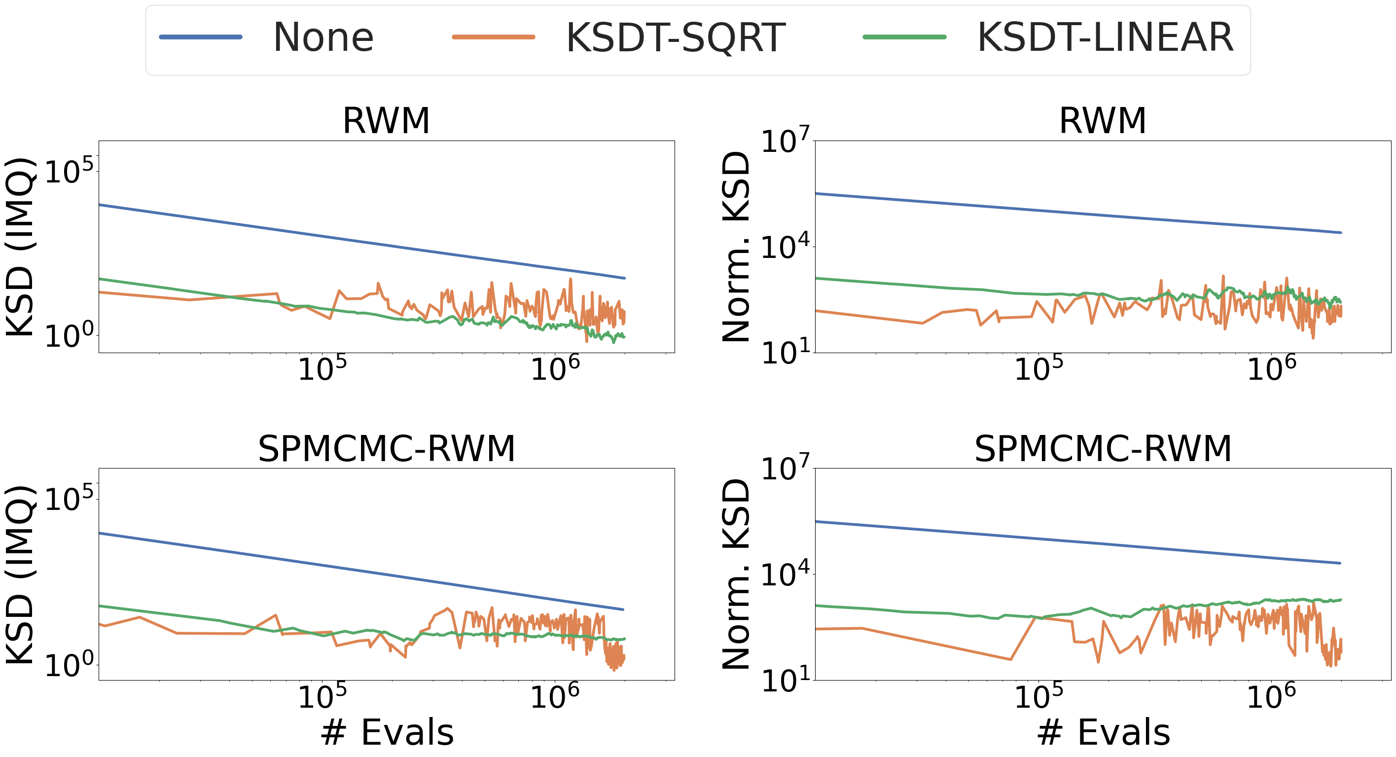
Figure 3: Goodwin oscillator problem with RWM and SPMCMC-RWM base samplers. Lower KSD and lower Normalized KSD are better. Axes are log-scale. Our KSDT-SQRT/LINEAR methods outperform the baseline methods on KSD and Normalized KSD.

The Goodwin Oscillator (Goodwin, 1965) is a well-studied test problem for Bayesian inference of ODE parameters (Calderhead & Girolami, 2009; Chen et al., 2019a; Riabiz et al., 2020). The task is to infer a 4-dimensional parameter that governs a genetic regulatory process specified by a system of coupled ODEs. See Appendix S5.2 of (Riabiz et al., 2020) for details. We use Random Walk Metropolis (RWM) and Metropolis-Adjusted Langevin Algorithm (MALA) chains of length $2\times 10^{6}$ taken from a public data repository which contains the sample chains used by (Riabiz et al., 2020). Since chains are pre-specified and all KSD-aware sample selection methods are deterministic, we do not present error bars for this experiment. In Figure 3 we report the results when applying KSD thinning to both the RWM chain and the RWM chain with the SPMCMC update rule applied. We follow the SPMCMC authors’ candidate set size of $m=10$ (see (10)) for this problem (Chen et al., 2019a). Our thinning methods outperform the baseline samplers on both KSD and Normalized KSD metrics. Our method with linear budget (KSDT-LINEAR) outperforms the square-root budget (KSDT-SQRT) on KSD but not normalized KSD due to the slower dictionary growth rate (smaller number of retained samples) of KSDT-SQRT. Results for the MALA and SPMCMC-MALA methods are reported in Appendix 7.1.

4.2 Calcium Signalling Model

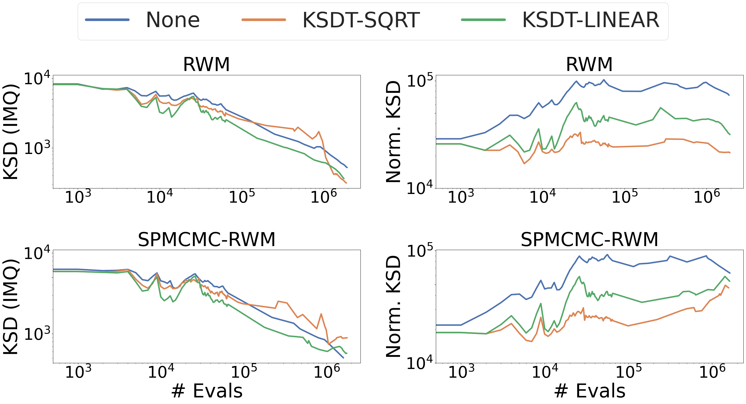
Figure 4: Calcium signalling model problem with tempered RWM and SPMCMC-RWM base samplers. Lower KSD and lower Normalized KSD are better. Axes are log-scale. Our methods outperform the baseline methods on Normalized KSD, and KSDT-LINEAR outperforms on KSD through most of the run.

We consider a calcium signaling model detailed in Appendix S5.4 of (Riabiz et al., 2020). The task is to infer a 38-dimensional parameter governing the signalling model. Uncertainty in the calcium signalling cascade parameter is used to propagate uncertainty to tissue-level simulations. The dataset consists of $4\times 10^{6}$ samples of the RWM sampler applied to a tempered posterior distribution. The samples are obtained from the same public repository as the Goodwin model samples. We set the SPMCMC parameter $m=100$ for this problem since many samples are duplicated due to MCMC rejection. This results in approximately $10$ unique samples per step. We report KSD and Normalized KSD results in Figure 4. We observe that KSDT-LINEAR outperforms the baseline sampler on both KSD and normalized KSD in all settings except for the tail end of the SPMCMC-RWM chain. Both KSDT-Linear and KSDT-SQRT outperform the baseline sampler after normalization based on sample complexity is taken into account.

4.3 Bayesian Neural Network Subspace Inference

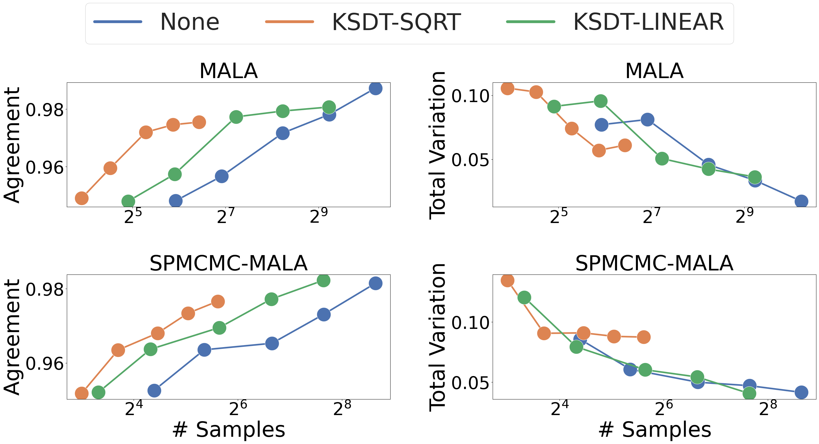
Figure 5: Agreement (left) and Total Variation (right) with the ground truth CIFAR-10 posterior predictive distribution. Higher Agreement and lower Total Variation indicate more accurate representations of the posterior predictive distribution. The x-axis is log-scale. Our KSDT-SQRT/LINEAR methods Pareto-dominate the baseline sampler on the Agreement metric and improve the low-sample Pareto frontier for the Total Variation metric.

Model complexity is a major challenge in sampling-based Bayesian deep learning. Each prediction on unseen test data requires one forward propagation per-sample so storage and inference costs grow linearly with the number of samples retained. In this section we demonstrate how our method improves the consistency vs. complexity Pareto frontier.

MCMC mixing is slow in high dimensions, so a popular technique is to find a low-dimensional subspace and perform Bayesian sampling in that subspace (Constantine et al., 2016; Cui et al., 2016; Izmailov et al., 2020a). Full subspace construction details are given in Appendix 7.3. We measure the quality of each sampling method’s approximation to the predictive distribution corresponding to the true posterior. We generate the ground truth predictive distribution by running 20,000 samples of SGLD (Welling & Teh, 2011), and follow (Izmailov et al., 2021) by measuring the top-1 agreement and total variation with respect to the ground truth predictive distribution. Total variation is

$$\frac{1}{n}\sum_{i=1}^{n}\frac{1}{2}\sum_{j=1}^{c}\left\lvert{p_{1}(\mathbf{y}_{i}=j|\mathbf{x}_{i})-p_{2}(\mathbf{y}_{i}=j|\mathbf{x}_{i})}\right\rvert$$ (17)

where $c$ is the number of classes. Higher agreement and lower total variation indicate higher-fidelity approximations to the ground truth predictive distribution. All results in this section are the mean over 5 chains. More details and additional experiments are given in Appendix 7.

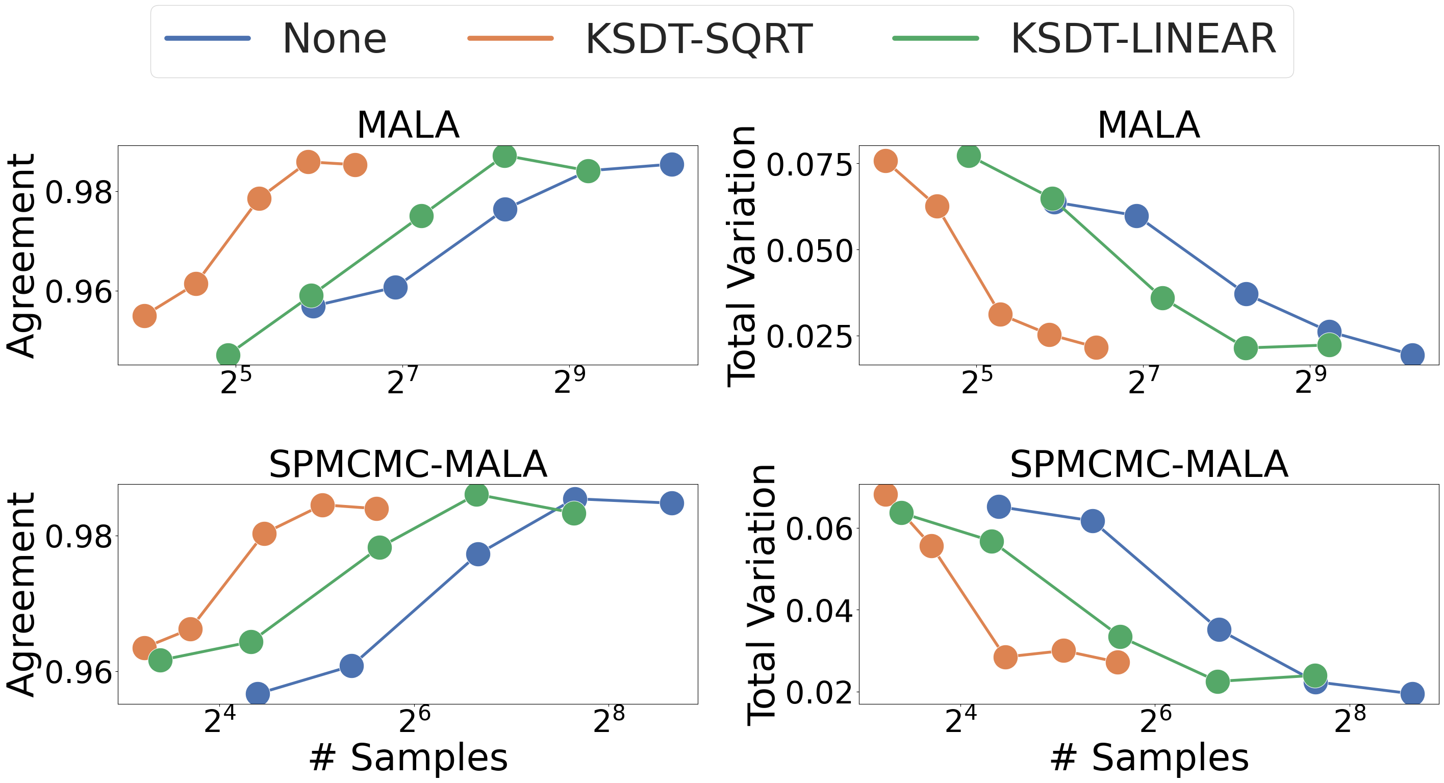
Figure 6: Agreement (left) and Total Variation (right) with the ground truth IMDB posterior predictive distribution. Higher Agreement and lower Total Variation indicate more accurate representations of the posterior predictive distribution. The x-axis is log-scale. Our KSDT-SQRT/LINEAR methods Pareto-dominate the baseline sampler on both the Agreement and Total Variation metrics.

CIFAR-10 Classification

The task is 10-class image classification, and we use a ResNet-20 with Filter Response Normalization from (Izmailov et al., 2021) as our base model. Our results in Figure 5 demonstrate that our online thinning method outperforms both the baseline sampler and SPMCMC-based samplers on the agreement metric. Improvement is mixed on the total variation metric, where our methods outperform existing methods in the low-sample regime, but have similar performance to existing methods once the model complexity is high.

IMDB Sentiment Prediction

The task is two-class sentiment prediction and we use a CNN-LSTM from (Izmailov et al., 2021) as our base model. Our results in Figure 6 demonstrate that all of our online thinning methods, in particular KSDT-SQRT, improve the Pareto frontier of the corresponding baseline sampler on both metrics. This conclusion holds across all sample regimes.

4.4 Automatic Adaptation to Target Complexity

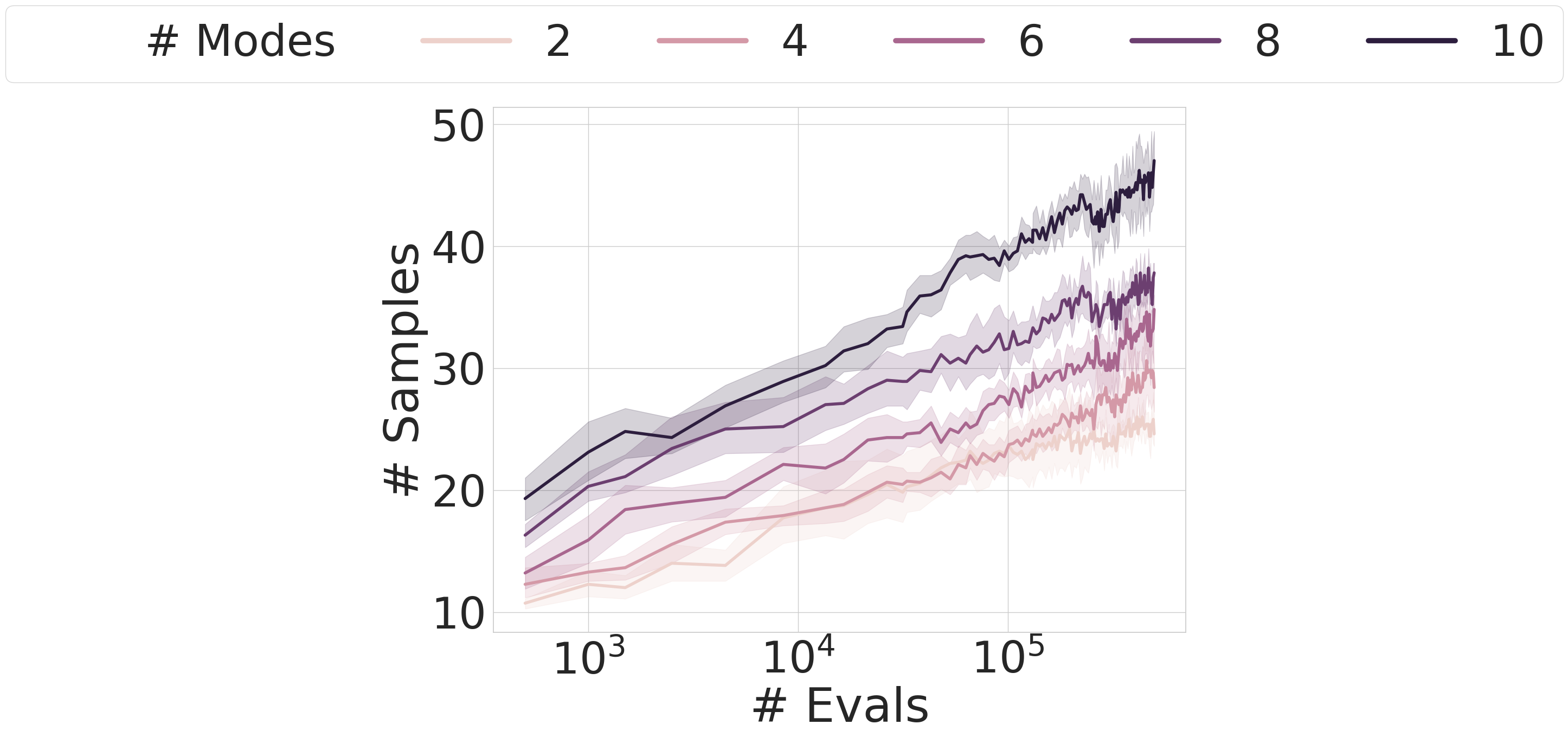
Figure 7: Thinning without mandatory dictionary size growth $f(i)=10$. Our algorithm automatically adapts to the number of modes by retaining 40 samples for a 10-mode mixture and 24 for a 4-mode mixture.

We have studied our KSD-Thinning algorithm with mandatory dictionary growth to ensure asymptotic consistency via Theorem 1. In this section we observe an interesting property of our algorithm: If we do not enforce model order growth, our thinning algorithm automatically adapts to the target distribution complexity. We target equally weighted Gaussian mixture models with an increasing number of modes and set $f(t)=10$. We match the setting of Theorem 1 and draw samples directly from the true distribution, applying the SPMCMC update rule with $m=5$. Figure 7 shows that the number of retained samples increases with the number of modes.

5 Conclusion

In this paper we presented an online thinning method that produces a compressed representation of a target distribution. Our work enables MCMC algorithms to directly target complexity-aware representations during, and can be applied to MCMC sampling scheme when gradients are available. We demonstrated the broad applicability of our method by comparing it to many baseline samplers in several problem settings, and found that it often improves model fit and reduces model complexity.

6 Convergence Results

We provide guarantees of convergence when the sample chain $\mathbf{S}$ is generated by SPCMCMC-style samplers. Our convergence results are provided in expectation, where the expectation $\mathbb{E}$ is taken with respect to the distribution underlying the sample generating process for $\mathbf{S}$. Specifically, the sample stream $\mathbf{S}$ is a sequence of random variables from a time-invariant distribution. Each realization of $\mathbf{S}$ is either a single MCMC sample chain, or the concatenation of several MCMC sample chains according to the SPMCMC update rule given in (10).

The two different sampling mechanisms that we consider are (1) i.i.d. sampling from the target distribution and (2) V-uniformly ergodic MCMC sampling. While we do not expect to directly draw samples from the true distribution, the i.i.d. sampling analysis is similar to the MCMC analysis and provides a simpler starting point. The decaying budget result from Theorem 1 is proven in two parts. Theorem 2 gives the desired result for i.i.d. sampling and Corollary 3 gives the desired result for the MALA sampler. A more general result for V-uniformly ergodic MCMC samplers is given in Theorem 3. The constant-budget result is given for i.i.d. sampling in Corollary 2 and for the MALA sampler in Corollary 4.

Symbol	Definition
$k_{0}$	Stein kernel as defined in (5)
$\mathcal{K}_{0}$	RKHS induced by Stein kernel
${\rm KSD}$	KSD as defined in (6)
$\mathcal{Y}_{i}$	search space for best next point to add
$\mathbf{x}_{n}$	new point added to dictionary $\mathbf{D}_{t-1}$ before projection step
$S_{n}$	“size” of search space $Y_{i}$
$h_{n}$	Optimal RKHS update given search space $\mathcal{Y}_{i}$
$\delta$	suboptimality incurred during search for KSD-optimal point
$r_{n}$	arbitrary positive constant
$m_{n}$	size of new point candidate set
$\{\mathbf{y}_{n,i}\}$	candidate set of MCMC samples
$\gamma,b$	constants used to bound exponentiated kernel

Table 3: Symbols used for convergence proofs

The following technical lemma imposes constraints on the sample stream $\mathbf{S}$. We will partition $\mathbf{S}$ into a sequence of batches $\mathcal{Y}_{i}$ and select the KSD-optimal element from each batch. The lemma below is stated for generic constants $S_{i},r_{i}$ and search sets $\mathcal{Y}_{i}$ to accommodate two cases (1) $\mathbf{S}$ is a stream of i.i.d samples from the target distribution (2) $\mathbf{S}$ is a stream of MCMC samples.

Lemma 1 (General Recursion Lemma, modified from Theorem 5 in (Chen et al., 2019b))

Let $\mathcal{X}$ be the domain of $p$. Fix $n\in\mathbb{N}$. Assume that for all $j\leq n$ the sequence of points $\{\mathbf{x}_{i}\}_{i=1}^{j}$, where $\mathbf{x}_{i}$ the greedy KSD-optimal point selected from the search space $\mathcal{Y}_{i}\subset\mathcal{X}$, satisfies

$$\frac{k_{0}(\mathbf{x}_{j},\mathbf{x}_{j})}{2}+\sum_{\mathbf{x}_{i}\in\mathbf{D}_{j-1}}k_{0}(\mathbf{x}_{i},\mathbf{x}_{j})\leq\frac{\delta}{2}+\frac{S_{j}^{2}}{2}+\inf_{\mathbf{x}\in\mathcal{Y}_{j}}\sum_{\mathbf{x}_{i}\in\mathbf{D}_{j-1}}k_{0}(\mathbf{x}_{i},\mathbf{x}).$$ (18)

Then for any constants $\delta>0$, $\{S_{i}\geq 0\}_{i=1}^{n}$, $\{r_{i}>0\}_{i=1}^{n}$ the thinned dictionary $\mathbf{D}_{n}=KSDT(\mathbf{D}_{n-1}\cup\{\mathbf{x}_{n}\},\epsilon_{n})$ satisfies

$${\rm KSD}(q_{\mathbf{D}_{n}})^{2}\leq\sum_{i=1}^{n-1}\left(\frac{\delta+S_{i}^{2}+r_{i}\|h_{i}\|_{\mathcal{K}_{0}}^{2}}{\left(|\mathbf{D}_{i-1}|+1\right)^{2}}+\epsilon_{i}\right)\left(\prod_{j=i}^{n-1}\frac{|\mathbf{D}_{j}|}{|\mathbf{D}_{j}|+1}\right)^{2}\left(\prod_{j=i}^{n-1}\left(1+\frac{1}{r_{j+1}}\right)\right)$$ (19)

where $h_{i}$ is any element of the Stein RKHS corresponding to points in the convex hull of $\mathcal{Y}_{i}$.

The main distinctions between Lemma 1 and Theorem 5 of (Chen et al., 2019b) is that we consider additional thinning through Algorithm 2. This thinning operation introduces the budget parameter $\epsilon_{i}$ (potential KSD increase) and the dictionary size $|\mathbf{D}_{j}|$ since the dictionary size is not a linear monotonically increasing function of the time step as in (Chen et al., 2019b)

Proof

The condition in (18) assumes that the point sequence $\{\mathbf{x}_{j}\}$ has bounded suboptimality $\delta$ with respect to KSD minimization at each step. Then the conclusion in (19) gives an upper bound on the squared KSD at step $n$. The general constants $\{S_{i}\},\{r_{i}\}$ will be instantiated based on the choice of search spaces $\{\mathcal{Y}_{i}\}$ and the choice of point generation method (MCMC, deterministic optimization, etc.).

First we will present a bound on the 1-step unthinned iterate. Next we account for KSD loss due to thinning to achieve a 1-step bound for our algorithm. Finally we recursively apply this bound to achieve the recurrence relation in (19).

First we provide a 1-step bound for the unthinned iterate $\tilde{\mathbf{D}}_{n}$ by adapting the proof style of Theorem 5 in Appendix A.1 of (Chen et al., 2019b) to suit our notation.

$$|\tilde{\mathbf{D}}_{n}|^{2}{\rm KSD}(q_{\tilde{\mathbf{D}}_{n}})^{2} =\sum_{\mathbf{x}_{i}\in\tilde{\mathbf{D}}_{n}}\sum_{x_{j}\in\tilde{\mathbf{D}}_{n}}k_{0}(\mathbf{x}_{i},\mathbf{x}_{j})$$

$$=|\mathbf{D}_{n-1}|^{2}{\rm KSD}(q_{\mathbf{D}_{n-1}})^{2}+k_{0}(\mathbf{x}_{n},\mathbf{x}_{n})+2\sum_{\mathbf{x}_{i}\in\mathbf{D}_{n-1}}k_{0}(\mathbf{x}_{i},\mathbf{x}_{n})$$

$$\leq|\mathbf{D}_{n-1}|^{2}{\rm KSD}(q_{\mathbf{D}_{n-1}})^{2}+\delta+S_{n}^{2}+2\inf_{\mathbf{x}\in\mathcal{Y}_{j}}\sum_{\mathbf{x}_{i}\in\mathbf{D}_{n-1}}k_{0}(\mathbf{x}_{i},\mathbf{x})$$ (20)

The equality follows from the definition of the KSD in (6). The second equality follows from the definition of the KSD again as we separate the elements in the final row and final column of the kernel matrix to get the second two terms. The last inequality is the direct application of the premise of Lemma 1, which ensures bounded suboptimality of the point $\mathbf{x}_{n}$, to the last two terms on the right-hand side of the middle equality in (20). Multiply the premise by 2 for direct application.

We apply the following result from Equation (11) of (Chen et al., 2019b):

$$2\inf_{x\in\mathcal{Y}_{j}}\sum_{\mathbf{x}_{i}\in\mathbf{D}_{n-1}}k_{0}(\mathbf{x}_{i},\mathbf{x})\leq r_{n}\|h_{n}\|^{2}_{\mathcal{K}_{0}}+\frac{{\rm KSD}(q_{\mathbf{D}_{n-1}})}{r_{n}}$$

to the last term on the right-hand side of (20) to get

$$|\tilde{\mathbf{D}}_{n}|^{2}{\rm KSD}(q_{\tilde{\mathbf{D}}_{n}})^{2}\leq|\mathbf{D}_{n-1}|^{2}\left(1+\frac{1}{r_{n}}\right){\rm KSD}(q_{\mathbf{D}_{n-1}})^{2}+\delta+S_{n}^{2}+r_{n}\|h_{n}\|_{\mathcal{K}_{0}}^{2}.$$ (21)

To recover the un-thinned KSD we divide both sides by both sides by $|\tilde{\mathbf{D}}_{n}|^{2}=\left(|\mathbf{D}_{n-1}|+1\right)^{2}$ to get

$${\rm KSD}(q_{\tilde{\mathbf{D}}_{n}})^{2}\leq\frac{|\mathbf{D}_{n-1}|^{2}}{\left(|\mathbf{D}_{n-1}|+1\right)^{2}}\left(1+\frac{1}{r_{n}}\right){\rm KSD}(q_{\mathbf{D}_{n-1}})^{2}+\frac{\delta+S_{n}^{2}+r_{n}\|h_{n}\|_{\mathcal{K}_{0}}^{2}}{\left(|\mathbf{D}_{n-1}|+1\right)^{2}}\\$$ (22)

We replace the un-thinned KSD ${\rm KSD}(q_{\tilde{\mathbf{D}}_{n}})^{2}$ with the thinned KSD ${\rm KSD}(q_{\mathbf{D}_{n}})^{2}$ and apply the stopping criterion of Algorithm  2 to establish the recurrence relationship

$${\rm KSD}(q_{\mathbf{D}_{n}})^{2}\leq\frac{|\mathbf{D}_{n-1}|^{2}}{\left(|\mathbf{D}_{n-1}|+1\right)^{2}}\left(1+\frac{1}{r_{n}}\right){\rm KSD}(q_{\mathbf{D}_{n-1}})^{2}+\frac{\delta+S_{n}^{2}+r_{n}\|h_{n}\|_{\mathcal{K}_{0}}^{2}}{\left(|\mathbf{D}_{n-1}|+1\right)^{2}}+\epsilon_{n}.$$ (23)

This recurrence may be unrolled backwards in time to write

$${\rm KSD}(q_{\mathbf{D}_{n}})^{2}\leq\sum_{i=1}^{n}\left(\frac{\delta+S_{i}^{2}+r_{i}\|h_{i}\|_{\mathcal{K}_{0}}^{2}}{\left(|\mathbf{D}_{i-1}|+1\right)^{2}}+\epsilon_{i}\right)\left(\prod_{j=i}^{n-1}\frac{|\mathbf{D}_{j}|}{|\mathbf{D}_{j}|+1}\right)^{2}\left(\prod_{j=i}^{n-1}\left(1+\frac{1}{r_{j+1}}\right)\right)$$ (24)

which upper bounds the error incurred by each step of the non-parametric approximation to the target density $p$, as stated in Lemma 1. $\blacksquare$

Next we present Lemma 2 which is a consequence of Lemma 1 when the KSD-optimal point selection is no longer generic, but instead the specific outcome of the SPMCMC update rule from (10) applied to the candidate discrete search space. For the following lemma, we assume that we are given a set of candidate samples from the target density $p$. We partition those samples into candidate sets $\mathcal{Y}_{i}=\{\mathbf{y}_{i,l}\}_{l=1}^{m_{i}}$ of size $m_{i}$. Then the sample stream $\mathbf{S}=\{\mathbf{x}_{i}\}_{i=1}^{\infty}$ is generated by the SPMCMC update from (10). The following lemma is a modified form of Theorem 6 from (Chen et al., 2019b).

Lemma 2 (Pruned Recursion with SPMCMC Update Rule)

Assume the same setup as Lemma  1. Using the SPMCMC update rule from (10) the iterate $\mathbf{D}_{n}=KSDT(\mathbf{D}_{n-1}\cup\{\mathbf{x}_{n}\},\epsilon_{n})$ satisfies

$${\rm KSD}(q_{\mathbf{D}_{n}})^{2}\leq\sum_{i=1}^{n}\left(\frac{S_{i}^{2}+r_{i}\|h_{i}\|_{\mathcal{K}_{0}}^{2}}{\left(|\mathbf{D}_{i-1}|+1\right)^{2}}+\epsilon_{i}\right)\left(\prod_{j=i}^{n-1}\frac{|\mathbf{D}_{j}|}{|\mathbf{D}_{j}|+1}\right)^{2}\left(\prod_{j=i}^{n-1}\left(1+\frac{1}{r_{j+1}}\right)\right)$$ (25)

Proof

In this proof we will apply Lemma  1 to this specific case by instantiating a specific constant $\delta$ related to the search procedure and bounding the search space $\mathcal{Y}_{i}$ with respect to $S_{i}$.

First we truncate and redefine the search set $\mathcal{Y}_{n}$ by restricting our attention to regions with kernel values bounded by $S_{n}^{2}$: $\mathcal{Y}_{n}=\{\mathbf{x}\in\mathcal{Y}_{n}\>|\>k_{0}(\mathbf{x},\mathbf{x})\leq S_{n}^{2}\}$. Then we note that the update rule in Equation 10 satisfies the premise ((18)) in Lemma 1 with $\delta=0$ because the infimum is a search over a finite set of points, and therefore the KSD suboptimality $\delta$ of the search procedure is $\delta=0$.

$$\frac{k_{0}(\mathbf{x}_{n},\mathbf{x}_{n})}{2}+\sum_{\mathbf{x}_{i}\in\mathbf{D}_{n-1}}k_{0}(\mathbf{x}_{i},\mathbf{x}_{n}) =\inf_{\mathbf{x_{n}}\in\mathcal{Y}_{n}}\frac{k_{0}(\mathbf{x}_{n},\mathbf{x}_{n})}{2}+\sum_{\mathbf{x}_{i}\in\mathbf{D}_{n-1}}k_{0}(\mathbf{x}_{i},\mathbf{x}_{n})$$

$$\leq\frac{S_{n}^{2}}{2}+\inf_{\mathbf{x}\in\mathcal{Y}_{n}}\sum_{\mathbf{x}_{i}\in\mathbf{D}_{n-1}}k_{0}(\mathbf{x}_{i},\mathbf{x})$$ (26)

The first equality follows from the optimality condition of the update rule (select the best point). The second line follows from the truncation criterion of $\mathcal{Y}_{n}$. Finally we can apply Lemma 1 with $\delta=0$ to achieve the desired conclusion in  (25). This concludes the proof of Lemma 2. $\blacksquare$

Lemma 1 is a stepping stone to Lemma 2. We use Lemma 2 to establish convergence of Algorithm 1 in the i.i.d. sampling setting of Theorem 2 by bounding the summation in (25) and therefore ensuring KSD convergence.

To achieve convergence we will require that the model order $|\mathbf{D}_{i}|$ is lower bounded by a monotone increasing function $f(i)\in\Omega\left(\sqrt{i\log(i)}\right)$. The lower bound on model order growth controls the convergence rate and influences maximum possible thinning budget $\{\epsilon_{i}\}$. This lower bound contrasts with the standard linear $|\mathbf{D}_{i}|=i$ growth rate for MCMC or i.i.d. sampling and the linear $f(i)\in\mathcal{O}(i)$ growth rate of (Chen et al., 2019b).

Theorem 2 (i.i.d Sampling and Decaying Thinning Budget)

Assume the same conditions as Lemma 2. Further assume that the kernel $k_{0}$ satisfies $\mathbb{E}_{\mathbf{y}\sim P}\left[e^{\gamma k_{0}(\mathbf{y},\mathbf{y})}\right]=b<\infty$, dictionary sizes are lower bounded as $|\mathbf{D}_{i}|\geq Cf(i)$ where $f(i)=\Omega\left(\sqrt{i\log(i)}\right)$ and that the compression budget $\{\epsilon_{i}\}$ is $\epsilon_{i}=\log(i)/f(i)^{2}$. Finally assume that the candidate samples $\{\mathbf{y}_{i,l}\}^{m_{i}}_{l}$ are drawn i.i.d from the target density $p$. Then the iterate $\mathbf{D}_{n}=KSDT(\mathbf{D}_{n-1}\cup\{\mathbf{x}_{n}\},\epsilon_{n})$ of Algorithm 1 satisfies

$$\mathbb{E}\left[{\rm KSD}(q_{\mathbf{D}_{n}})^{2}\right]\leq C\frac{n\log(n)}{f(n)^{2}}.$$ (27)

Proof

To complete our proof of convergence first we will split the recurrence from Lemma  1 into two terms, one corresponding to the sampling error and one corresponding to the thinning error. Then we will bound each individually by selecting specific values of $\{r_{i}\},\{S_{i}\}$ and $\{m_{i}\}$ and applying a bound for $\|h_{i}\|_{\mathcal{K}_{0}}$.

First we apply standard log-sum-exp bound as in (Chen et al., 2019b) the part related to the sampling error to write

$$\prod_{j=i}^{n-1}\left(1+\frac{1}{r_{j+1}}\right)\leq\exp\left(\sum_{j=1}^{n}\frac{1}{r_{j}}\right).$$ (28)

We substitute (28) into the conclusion of Lemma 2 to get

$$\begin{split}\mathbb{E}\left[{\rm KSD}(q_{\mathbf{D}_{n}})^{2}\right]&\leq\mathbb{E}\left[\exp\left(\sum_{j=1}^{n}\frac{1}{r_{j}}\right)\sum_{i=1}^{n}\left(\frac{S_{i}^{2}+r_{i}\|h_{i}\|_{\mathcal{K}_{0}}^{2}}{\left(|\mathbf{D}_{i-1}|+1\right)^{2}}+\epsilon_{i}\right)\left(\prod_{j=i}^{n-1}\frac{|\mathbf{D}_{j}|}{|\mathbf{D}_{j}|+1}\right)^{2}\right]\\ \end{split}$$ (29)

For now we ignore the leading exponential and decompose the summation into two terms related to the sampling and compression-based error, respectively, as:

$$\begin{split}\sum_{i=1}^{n}&\left(\frac{S_{i}^{2}+r_{i}\|h_{i}\|_{\mathcal{K}_{0}}^{2}}{\left(|\mathbf{D}_{i-1}|+1\right)^{2}}+\epsilon_{i}\right)\left(\prod_{j=i}^{n-1}\frac{|\mathbf{D}_{j}|}{|\mathbf{D}_{j}|+1}\right)^{2}\\ &=\underbrace{\sum_{i=1}^{n}\left(\frac{S_{i}^{2}+r_{i}\|h_{i}\|_{\mathcal{K}_{0}}^{2}}{\left(|\mathbf{D}_{i-1}|+1\right)^{2}}\right)\left(\prod_{j=i}^{n-1}\frac{|\mathbf{D}_{j}|}{|\mathbf{D}_{j}|+1}\right)^{2}}_{T_{1}}+\underbrace{\sum_{i=1}^{n}\epsilon_{i}\left(\prod_{j=i}^{n-1}\frac{|\mathbf{D}_{j}|}{|\mathbf{D}_{j}|+1}\right)^{2}}_{T_{2}}\end{split}$$ (30)

The term $T_{1}$ is the bias incurred at each step of the unthinned point selection scheme. The term $T_{2}$ is the bias incurred by the thinning operation carried out at each step.

Bound on $T_{1}$

The term $T_{1}$ is the bias incurred by the point sampling scheme.

$$\begin{split}\mathbb{E}\Bigg{[}\sum_{i=1}^{n}\left(\frac{S_{i}^{2}+r_{i}\|h_{i}\|_{\mathcal{K}_{0}}^{2}}{\left(|\mathbf{D}_{i-1}|+1\right)^{2}}\right)&\left(\prod_{j=i}^{n-1}\frac{|\mathbf{D}_{j}|}{|\mathbf{D}_{j}|+1}\right)^{2}\Bigg{]}\\ &=\mathbb{E}\left[\sum_{i=1}^{n}\left(\frac{S_{i}^{2}+r_{i}\|h_{i}\|_{\mathcal{K}_{0}}^{2}}{\left(|\mathbf{D}_{n-1}|+1\right)^{2}}\right)\left(\prod_{j=i}^{n-1}\frac{|\mathbf{D}_{j}|}{|\mathbf{D}_{j-1}|+1}\right)^{2}\right]\\ &\leq\mathbb{E}\left[\sum_{i=1}^{n}\frac{S_{i}^{2}+r_{i}\|h_{i}\|_{\mathcal{K}_{0}}^{2}}{\left(|\mathbf{D}_{n-1}|+1\right)^{2}}\right]\\ &C\sum_{i=1}^{n}\frac{S_{i}^{2}+r_{i}\mathbb{E}\left[\|h_{i}\|_{\mathcal{K}_{0}}^{2}\right]}{f(n)^{2}}\end{split}$$ (31)

The first equality is a re-arrangement of the denominators that pulls in the term $\frac{1}{(|\mathbf{D}_{i-1}|+1)^{2}}$. The second inequality is a consequence of the fact that $|\mathbf{D}_{j}|\leq|\mathbf{D}_{j-1}|+1$ so each product of the dictionary order ratios is at most 1. The final term is based on the assumption of dictionary model order growth, i.e., $|\mathbf{D}_{n}|\geq f(n)$. From Appendix A, Equation (17) of (Chen et al., 2019b) we can apply truncated kernel mean embeddings and the fact that the points are drawn i.i.d. from the true distribution $P$ to bound $\mathbb{E}\left[\|h_{i}\|_{\mathcal{K}_{0}}^{2}\right]$ by

$$\mathbb{E}\left[\|h_{i}\|_{\mathcal{K}_{0}}^{2}\right]\leq\frac{4b}{\gamma}e^{-\frac{\gamma}{2}S_{i}^{2}}+\frac{4}{m_{j}}S_{i}^{2}$$ (32)

which relies on the assumption that $k_{0}$ satisfies $\mathbb{E}_{\mathbf{y}\sim P}\left[e^{\gamma k_{0}(\mathbf{y},\mathbf{y})}\right]=b<\infty$. Therefore

$$\mathbb{E}\Bigg{[}\sum_{i=1}^{n}\left(\frac{S_{i}^{2}+r_{i}\|h_{i}\|_{\mathcal{K}_{0}}^{2}}{\left(|\mathbf{D}_{i-1}|+1\right)^{2}}\right) \left(\prod_{j=i}^{n-1}\frac{|\mathbf{D}_{j}|}{|\mathbf{D}_{j}|+1}\right)^{2}\Bigg{]}$$

$$\leq C\frac{1}{f(n)^{2}}\sum_{i=1}^{n}\left((1+\frac{r_{i}}{m_{i}})S_{i}^{2}+r_{i}e^{-\frac{\gamma}{2}S_{i}^{2}}\right)$$ (33)

The inequality is an application of (32) to the final conclusion of (31) followed by an absorption of the constants into $C$. Note that $C\propto\exp{\sum_{i=1}^{n}\frac{1}{r_{i}}}$. We follow (Chen et al., 2019b) and select and choose $S_{i}=\sqrt{\frac{2}{\gamma}\log(n\wedge m_{i})}$ and $r_{i}=n$. The selection $r_{i}=n$ is necessary to ignore the leading exponential $\exp\left(\sum_{j=1}^{n}\frac{1}{r_{j}}\right)$ and render that term constant. The choices of $r_{i}$ and $S_{i}$ are artefacts of the analysis, but do not affect the practical algorithm. Set $m_{i}=n$ to get

$$\mathbb{E}\Bigg{[}\sum_{i=1}^{n}\left(\frac{S_{i}^{2}+r_{i}\|h_{i}\|_{\mathcal{K}_{0}}^{2}}{\left(|\mathbf{D}_{i-1}|+1\right)^{2}}\right) \left(\prod_{j=i}^{n-1}\frac{|\mathbf{D}_{j}|}{|\mathbf{D}_{j}|+1}\right)^{2}\Bigg{]}$$

$$\leq C\frac{1}{f(n)^{2}}\sum_{i=1}^{n}\left(\log(n)+1\right)$$

$$\leq C\frac{n\log(n)}{f(n)^{2}}.$$ (34)

The first inequality is the conclusion of the previous equation with $S_{i}$ and $r_{i}$ evaluated and all constants absorbed. The second inequality holds because the summand does not depend on the index so we can multiply by $n$. This completes the bound on $T_{1}$ subject to the dictionary growth constraint.

Bound on $T_{2}$

The term $T_{2}$ is the bias incurred by the thinning operation. We will tune the budget schedule $\{\epsilon_{i}\}$ so that $T_{2}$ tends to 0 at the same rate as $T_{1}$. The goal is to keep epsilon as large as possible in order to retain as few points as possible while preserving the rate of posterior contraction. Noticeably, we do not need this term to converge any faster than $n\log n/f(n)^{2}$. The only dependence on the point stream $\mathbf{S}$ comes from $|\mathbf{D}_{j}|$, and we directly bound this term by observing that $|\mathbf{D}_{j}|\leq j$ so

$$\frac{|\mathbf{D}_{j}|}{|\mathbf{D}_{j+1}|}\leq\frac{j}{j+1}.$$

Therefore, returning to $T_{2}$ in (30), we have

$$\mathbb{E}\left[\sum_{i=1}^{n}\epsilon_{i}\left(\prod_{j=i}^{n-1}\frac{|\mathbf{D}_{j}|}{|\mathbf{D}_{j}|+1}\right)^{2}\right] \leq\sum_{i=1}^{n}\epsilon_{i}\left(\prod_{j=i}^{n-1}\frac{j}{j+1}\right)^{2}$$

$$=\sum_{i=1}^{n}\epsilon_{i}\frac{i^{2}}{n^{2}}$$

$$=\frac{1}{n^{2}}\sum_{i=1}^{n}\epsilon_{i}i^{2}$$ (35)

Therefore the goal is to choose $\epsilon_{i}$ satisfying (up to generic constants)

$$\frac{1}{n^{2}}\sum_{i=1}^{n}\epsilon_{i}i^{2} \leq\frac{n\log n}{f(n)^{2}}$$

$$\iff\sum_{i=1}^{n}\epsilon_{i}i^{2} \leq\frac{n^{3}\log n}{f(n)^{2}}$$ (36)

The first line above states that $T_{1}$ and $T_{2}$ converge at the same rate. The second line simply multiplies the first inequality by $n^{2}$. Therefore, to satisfy the condition on the right-hand side of the previous expression, one can select $\epsilon_{i}$ according to the growth condition associated with the posterior contraction rate of the sampled process, i.e., the upper bound on $T_{1}$ in (50). According to this rate, the model complexity increases at least according to the growth rate $f(i)$. We set $\epsilon_{i}=\log(i)/f(i)^{2}$ and demonstrate that (6) is met:

$$\begin{split}\sum_{i=1}^{n}\epsilon_{i}i^{2}&=\sum_{i=1}^{n}\frac{i^{2}\log(i)}{f(i)^{2}}\\ &\leq\sum_{i=1}^{n}\frac{n^{2}\log(n)}{f(n)^{2}}\\ &=\frac{n^{3}\log(n)}{f(n)^{2}}\\ \end{split}$$ (37)

The first line is the evaluation of $\epsilon_{i}$. The inequality in the second line holds because $f(i)\leq i$ so the summand is increasing in $i$. After we remove the dependence on the index $i$ we multiply by the maximum summation index $n$ to achieve the desired result. This concludes the bound of $T_{2}$.

Finally we can substitute the bound for $T_{1}$ ((34)) and the bound for $T_{2}$ ((37)) into (30) to get

$$\mathbb{E}\left[\sum_{i=1}^{n}\left(\frac{S_{i}^{2}+r_{i}\|h_{i}\|_{\mathcal{K}_{0}}^{2}}{\left(|\mathbf{D}_{i-1}|+1\right)^{2}}+\epsilon_{i}\right)\left(\prod_{j=i}^{n-1}\frac{|\mathbf{D}_{j}|}{|\mathbf{D}_{j}|+1}\right)^{2}\right]\leq C\frac{n\log(n)}{f(n)^{2}}.$$ (38)

Finally we revisit (29) to achieve our desired conclusion:

$$\begin{split}\mathbb{E}\left[{\rm KSD}(q_{\mathbf{D}_{n}})^{2}\right]&\leq\mathbb{E}\left[\exp\left(\sum_{j=1}^{n}\frac{1}{r_{j}}\right)\sum_{i=1}^{n}\left(\frac{S_{i}^{2}+r_{i}\|h_{i}\|_{\mathcal{K}_{0}}^{2}}{\left(|\mathbf{D}_{i-1}|+1\right)^{2}}+\epsilon_{i}\right)\left(\prod_{j=i}^{n-1}\frac{|\mathbf{D}_{j}|}{|\mathbf{D}_{j}|+1}\right)^{2}\right]\\ &=\mathbb{E}\left[e\sum_{i=1}^{n}\left(\frac{S_{i}^{2}+r_{i}\|h_{i}\|_{\mathcal{K}_{0}}^{2}}{\left(|\mathbf{D}_{i-1}|+1\right)^{2}}+\epsilon_{i}\right)\left(\prod_{j=i}^{n-1}\frac{|\mathbf{D}_{j}|}{|\mathbf{D}_{j}|+1}\right)^{2}\right]\\ &\leq C\frac{n\log(n)}{f(n)^{2}}\\ \end{split}$$ (39)

The equality in the second line follows from the fact that $r_{j}=n$ for all $j$. The final inequality follows from an application of (38) to reach the desired conclusion of Theorem 2. $\blacksquare$

Corollary 2 (i.i.d. Convergence with constant thinning budget)

Fix the desired KSD convergence radius $\Delta$. Assume that the dictionary model order growth rate $f$ takes the parametric form $f(i)=\sqrt{i^{1+\alpha}\log(i)}$ with $1<\alpha<2$. With constant thinning budget $\epsilon=\mathcal{O}\left(\Delta^{1+\frac{1}{\alpha}}\right)$, after $n=\mathcal{O}\left(\frac{1}{\Delta^{\frac{1}{\alpha}}}\right)$ steps the KSD satisfies

$$\mathbb{E}\left[{\rm KSD}\left(q_{\mathbf{D}_{n}}\right)^{2}\right]\leq C\Delta$$ (40)

for some generic constant $C$. Equivalently, if we fix a constant thinning budget $\epsilon$, after $n=\mathcal{O}\left(\epsilon^{-\frac{2}{\alpha+1}}\right)$ steps the KSD satisfies

$$\mathbb{E}\left[{\rm KSD}\left(q_{\mathbf{D}_{n}}\right)^{2}\right]\leq C\epsilon^{\frac{2}{1+\frac{1}{\alpha}}}$$ (41)

Proof

We will revisit terms $T_{1}$ and $T_{2}$ in (30) from the proof of Theorem 2 and show how to obtain the desired convergence rate in the constant thinning budget regime.

First, (34) demonstrates that the sampling error term $T_{1}$ converges at a rate of $\frac{n\log(n)}{f(n)^{2}}$ (up to generic constants). We set the convergence rate equal to the convergence radius and apply algebraic manipulations to derive the number of sampling and thinning iterations required. In particular, write:

$$\Delta=\frac{n\log(n)}{f(n)^{2}}=\frac{n\log(n)}{n^{1+\alpha}\log(n)}=\frac{1}{n^{\alpha}}$$ (42)

Since the convergence rate $\frac{n\log(n)}{f(n)^{2}}$ holds up to generic constants we can conclude that after $n=\mathcal{O}\left(\frac{1}{\Delta^{\frac{1}{\alpha}}}\right)$ steps $T_{1}\leq C\Delta$.

Next we bound $T_{2}$, the error associated with memory-reduction. We demonstrated in the proof of Theorem 2 that

$$T_{2}\leq\frac{1}{n^{2}}\sum_{i=1}^{n}\epsilon_{i}i^{2}.$$ (43)

Since $\epsilon_{i}=\epsilon=\mathcal{O}\left(\Delta^{1+\frac{1}{\alpha}}\right)$ is constant with respect to the summation index $i$, we can evaluate the expression above as

$$\begin{split}\frac{1}{n^{2}}\sum_{i=1}^{n}\epsilon_{i}i^{2}&=\frac{\Delta^{1+\frac{1}{\alpha}}}{n^{2}}\sum_{i=1}^{n}i^{2}\\ &\leq\frac{\Delta^{1+\frac{1}{\alpha}}}{n^{2}}Cn^{3}\\ &=Cn\Delta^{1+\frac{1}{\alpha}}\\ &=C\frac{\Delta^{1+\frac{1}{\alpha}}}{\Delta^{\frac{1}{\alpha}}}=C\Delta\end{split}$$ (44)

In the first line we plug in $\epsilon$. In the second line we make use of the general summation formula $\sum_{i=1}^{n}i^{2}=\frac{n(n+1)(n+2)}{6}\leq Cn^{3}$. In the final line we apply the fact that $n=\mathcal{O}\left(\frac{1}{\Delta^{\frac{1}{\alpha}}}\right)$ and conclude that $T_{2}\leq C\Delta$ for some generic constant $C$.

Therefore we have $T_{1}+T_{2}\leq C\Delta$ which is the desired conclusion. $\blacksquare$

Next we consider the case when samples are generated using any MCMC sampling procedure. The one constraint we place on the sampler is that it exhibits geometric convergence with respect to a given function $V$. The function $V$, which controls the rate of geometric convergence, will contribute to the sampling errror term $T_{1}$ in our analysis.

Definition 3

A Markov chain $\{\mathbf{y}_{n}\}\subset\mathcal{X}$ with $n$-th step transition kernel $P^{n}$ is $V$-uniformly ergodic for a positive function $V:\mathcal{X}\rightarrow[1,\infty]$ if there exists $R\in[0,\infty],\rho\in(0,1)$ such that

$$\sup_{\mathbf{x}\in X}\frac{\|P^{n}(\mathbf{y},\mathbf{x})-p(\mathbf{x})\|}{V(\mathbf{x})}\leq RV(\mathbf{y})p^{n}$$ (45)

We introduce new notation from (Chen et al., 2019b) by defining the function $V_{\pm}$:

$$V_{\pm}(s)=\sup_{\mathbf{x}:k_{0}(\mathbf{x},\mathbf{x})\leq s^{2}}k_{0}(\mathbf{x},\mathbf{x})^{1/2}V(x)^{\pm 1}$$ (46)

We will use these two functions $V_{\pm}$ and a result from (Chen et al., 2019b) to control the sampling error of a $V$-uniformly ergodic Markov chain. First we extend the convergence guarantees of Algorithm 1 to general $V$-uniformly ergodic samplers in Theorem 3. Then, when MALA is $V$-uniformly ergodic, the desired result follows.

Theorem 3 (V-Uniformly Ergodic MCMC Sampling and Decaying Budget)

Suppose the same conditions as Lemma  2, and the Stein kernel $k_{0}$ satisfies $\mathbb{E}_{\mathbf{y}\sim P}\left[e^{\gamma k_{0}(\mathbf{y},\mathbf{y})}\right]=b<\infty$, and the lower-bound on the dictionary growth condition $|\mathbf{D}_{i}|\geq Cf(i)$ holds where $f(i)=\Omega\left(\sqrt{i\log(i)}\right)$, with compression budgets set as $\epsilon_{i}=\frac{\log(i)}{f(i)^{2}}$. Further assume that the candidate samples in each $\{\mathbf{y}_{i,l}^{m_{i}}\}$ are produced by a V-uniformly ergodic markov chain. Then the iterate $\mathbf{D}_{n}=KSDT(\mathbf{D}_{n-1}\cup\{\mathbf{x}_{n}\},\epsilon_{n})$ satisfies

$$\mathbb{E}\left[{\rm KSD}(q_{\mathbf{D}_{n}})^{2}\right]\leq C\left(\frac{n\log(n)}{f(n)^{2}}+\frac{1}{nf(n)^{2}}\sum_{i=1}^{n}V_{+}(S_{i})V_{-}(S_{i})\right)$$ (47)

Proof

This proof is similar to the proof of Theorem 2. It differs only in the bound applied to the term $\|h_{j}\|_{\mathcal{K}_{0}}^{2}$ which is a subcomponent of the sampling bias term $T_{1}$. This difference is due to the non-i.i.d. sampling procedure used to generate candidate samples that in turn define $h_{j}$. When the candidate samples $\{\mathbf{y}_{i,l}\}^{m_{i}}_{l=1}$ are generated from a $V$-uniformly ergodic markov chain, we can apply the following bound from (Chen et al., 2019b)[Appendix A.2, Equation (22)]:

$$\mathbb{E}\left[\|h_{j}\|_{\mathcal{K}_{0}}^{2}\right]\leq\frac{4b}{\gamma}\exp\left({-\frac{\gamma}{2}S_{j}^{2}}\right)+2RV_{+}(S_{j})V_{-}(S_{j})\left(\frac{1+2p}{1-p}\right)\frac{1}{m_{j}}$$ (48)

where the constants $p$ and $R$ come from the $V$-uniform ergodicity of the Markov chain that generates the candidate samples.

Our goal is to mimic the conclusion of (6) in our current setting.

$$\mathbb{E}\Bigg{[}\sum_{i=1}^{n} \left(\frac{S_{i}^{2}+r_{i}\|h_{i}\|_{\mathcal{K}_{0}}^{2}}{\left(|\mathbf{D}_{i-1}|+1\right)^{2}}\right)\left(\prod_{j=i}^{n-1}\frac{|\mathbf{D}_{j}|}{|\mathbf{D}_{j}|+1}\right)^{2}\Bigg{]}$$

$$\leq C\frac{1}{f(n)^{2}}\sum_{i=1}^{n}\left(S_{i}^{2}+r_{i}\exp\left(-\frac{\gamma}{2}S_{i}^{2}\right)+\frac{V_{+}(S_{i})V_{-}(S_{i})}{m_{j}}\right)$$ (49)

The first inequality is an application of (48) to the final conclusion of (31) from the proof of Theorem 2. We also absorb the constant factors into $C$. We select $S_{i}=\sqrt{\frac{2}{\gamma}\log(n\wedge m_{i})}$, $r_{i}=n$, and $m_{i}=n$ to achieve the bound

$$\mathbb{E}\Bigg{[}\sum_{i=1}^{n}\left(\frac{S_{i}^{2}+r_{i}\|h_{i}\|_{\mathcal{K}_{0}}^{2}}{\left(|\mathbf{D}_{i-1}|+1\right)^{2}}\right) \left(\prod_{j=i}^{n-1}\frac{|\mathbf{D}_{j}|}{|\mathbf{D}_{j}|+1}\right)^{2}\Bigg{]}$$

$$\leq C\frac{1}{f(n)^{2}}\sum_{i=1}^{n}\left(\log(n)+\frac{V_{+}(S_{i})V_{-}(S_{i})}{n}\right)$$

$$\leq C\left(\frac{n\log(n)}{f(n)^{2}}+\frac{1}{nf(n)^{2}}\sum_{i=1}^{n}V_{+}(S_{i})V_{-}(S_{i})\right)$$ (50)

The first inequality is the conclusion of the previous equation with $S_{i}$, and $r_{i}$ evaluated and all constants absorbed. The second inequality holds because the summand does not depend on the index so we can multiply by $n$. This completes the bound on $T_{1}$ in the setting where samples are generated by a V-uniformly ergodic Markov chain.

The bound on $T_{2}$ in Theorem 2 does not depend on the sample generation mechanism, so we can draw the same conclusion as (37) which does not introduce any terms with higher asymptotic growth order than $n\log(n)/f(n)^{2}$. Therefore the bound from (50) is the asymptotic upper bound, and we have achieved the desired result. $\blacksquare$

Our goal is to show that using MALA to generate samples ensures convergence of Algorithm 1. When MALA is inwardly convergent, MALA is $V$-uniformly ergodic. We make use of this fact to add one more condition (inwardly convergent) and present a convergence result for Algorithm 1 using the MALA sampler.

Corollary 3 (MALA Convergence with Decaying Budget)

Assume that the candidate sample sets $\{\mathbf{y}_{i,l}\}_{l=1}^{m_{i}}$ are generated by the Metropolis-Adjusted Langevin Algorithm (MALA) transition kernel with stepsize $h$ and that MALA is inwardly convergent for the target density $p$. Further assume that $p$ is distantly dissipative. Then the iterates $\mathbf{D}_{n}$ of Algorithm 1 satisfy

$$\mathbb{E}\left[{\rm KSD}(q_{\mathbf{D}_{n}})^{2}\right]\leq C\left(\frac{n\log(n)}{f(n)^{2}}\right)$$

Proof

We make use of two results from (Chen et al., 2019b), Appendix A.3. First we use the fact that MALA is inwardly convergent to conclude that MALA is $V$-uniformly ergodic with $V(\mathbf{x})=1+\|x\|_{2}$. The second result is the set of bounds $V_{+}(s)\leq C(s+s^{2})$ and $V_{-}(s)\leq C$ for some generic constant $C$. Then we can plug in $S_{i}=\sqrt{\frac{2}{\gamma}\log(n)}$ (since $m_{i}=n$) to bound the second term in Equation 50:

$$\frac{1}{nf(n)^{2}} \sum_{i=1}^{n}V_{+}(S_{i})V_{-}(S_{i})$$

$$\leq\frac{C}{nf(n)^{2}}\sum_{i=1}^{n}\left(S_{i}+S_{i}^{2}\right)$$

$$\leq\frac{C}{nf(n)^{2}}\sum_{i=1}^{n}\left(\sqrt{\log(n)}+\log(n)\right)$$

$$\leq\frac{C\sqrt{log(n)}+\log(n)}{f(n)^{2}}$$

$$\leq\frac{C\log(n)}{f(n)^{2}}$$ (51)

The first inequality is result of the evaluation of $V_{\pm}(S_{i})$ and the absorption of constants. The second inquality is the results of the evaluation of $S_{i}=\sqrt{\frac{2}{\gamma}\log(n)}$ and the absorption of constants. The third inequality follows from the fact that the summand does not depend on the index. The final inequality is an application of the fact that $\sqrt{\log(n)}\leq\log(n)$ for $n\geq 10$, which we assume as a reasonable minimum number of steps.

Since the final term in (51) is asymptotically upper bounded by $n\log(n)/f(n)^{2}$ due to the extra factor of $n$ we can ignore this term in Equation 47 and draw the desired conclusion that

$$\mathbb{E}\left[{\rm KSD}(q_{\mathbf{D}_{n}})^{2}\right]\leq C\left(\frac{n\log(n)}{f(n)^{2}}\right)$$ (52)

$\blacksquare$

Corollary 4 (MALA Convergence with constant thinning budget)

Fix the desired KSD convergence radius $\Delta$. Assume that the dictionary model order growth rate $f$ takes the parametric form $f(i)=\sqrt{i^{1+\alpha}\log(i)}$ with $1<\alpha<2$. With constant thinning budget $\epsilon=\mathcal{O}\left(\Delta^{1+\frac{1}{\alpha}}\right)$, after $n=\mathcal{O}\left(\frac{1}{\Delta^{\frac{1}{\alpha}}}\right)$ steps the KSD satisfies

$$\mathbb{E}\left[{\rm KSD}\left(q_{\mathbf{D}_{n}}\right)^{2}\right]\leq c\Delta$$ (53)

for some generic constant $C$. Equivalently, if we fix a constant thinning budget $\epsilon$, after $n=\mathcal{O}\left(\epsilon^{-\frac{2}{\alpha+1}}\right)$ steps the KSD satisfies

$$\mathbb{E}\left[{\rm KSD}\left(q_{\mathbf{D}_{n}}\right)^{2}\right]\leq C\epsilon^{\frac{2}{1+\frac{1}{\alpha}}}$$ (54)

This proof is exactly the same as the proof of Corollary 2 since the asymptotic convergence rate achieved in Corollary 3 is exactly the same as in the i.i.d. case in Theorem 2. We note that the convergence rate from Corollary 4 also trivially extends to the general case of V-uniformly ergodic samplers using the result of Theorem 3 and the analysis of Corollary 1.

7 Additional Experiments

In the main body we focused on results using the IMQ base kernel for the KSD. In this Appendix section we report results for the RBF kernel and additional metrics for both the IMQ and RBF kernels. We also provide per-sampler figures so that readers can easily evaluate the affect of our approach on individual samplers. We keep the same experimental settings as in the main body of the text. We follow (Detommaso et al., 2018) and set the kernel bandwith $h$ as the problem dimension $h=dim(\mathbf{x})$ when using the RBF kernel.

7.1 Goodwin Oscillator

We report the results on a per-sampler basis when applying KSD thinning to both the RWM chain and the MALA chains with and without the SPMCMC update rule using either the RBF or IMQ kernels in Figures 8,10,9, and 11. In all cases the conclusions are similar to those we draw from Figure 3 in the main body. Removing samples using our KSDT-LINEAR and KSDT-SQRT methods improves both KSD and normalized KSD.

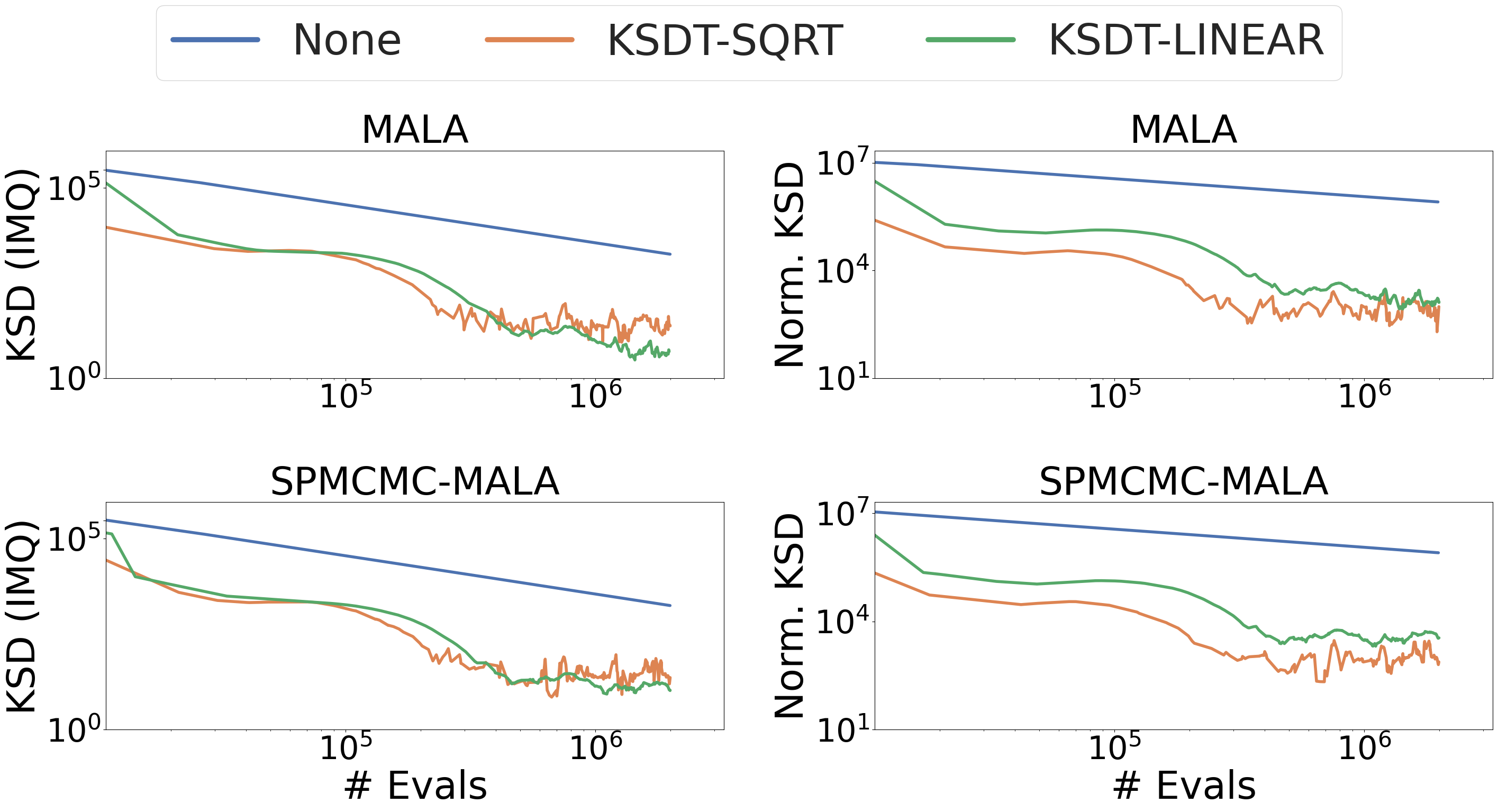
Figure 8: Goodwin problem, IMQ base kernel. Comparison of un-thinned sample chains from the MALA and SPMCMC-MALA samplers with our thinning methods KSDT-SQRT and KSDT-LINEAR. Lower KSD and lower Normalized KSD indicate more accurate representations of the target distribution. Both axes are log-scale. Our methods outperform the baseline methods on both KSD and Normalized KSD.

Figure 9: Goodwin problem, IMQ base kernel. Comparison of un-thinned sample chains from the RWM and SPMCMC-RWM samplers with our thinning methods KSDT-SQRT and KSDT-LINEAR. Lower KSD and lower Normalized KSD indicate more accurate representations of the target distribution. Both axes are log-scale. Our methods outperform the baseline methods on both KSD and Normalized KSD.

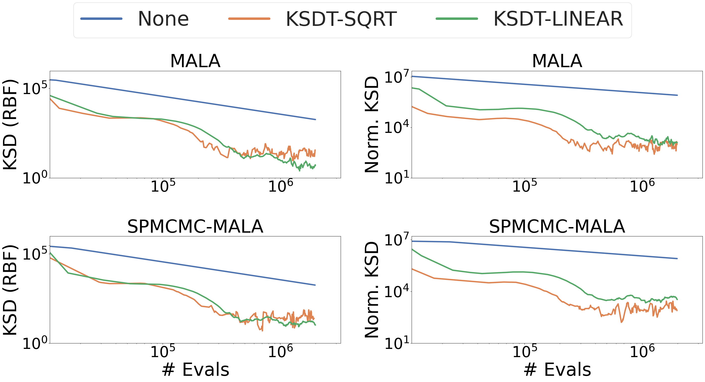
Figure 10: Goodwin problem, RBF base kernel. Comparison of un-thinned sample chains from the MALA and SPMCMC-MALA samplers with our thinning methods KSDT-SQRT and KSDT-LINEAR. Lower KSD and lower Normalized KSD indicate more accurate representations of the target distribution. Both axes are log-scale. Our methods outperform the baseline methods on both KSD and Normalized KSD.

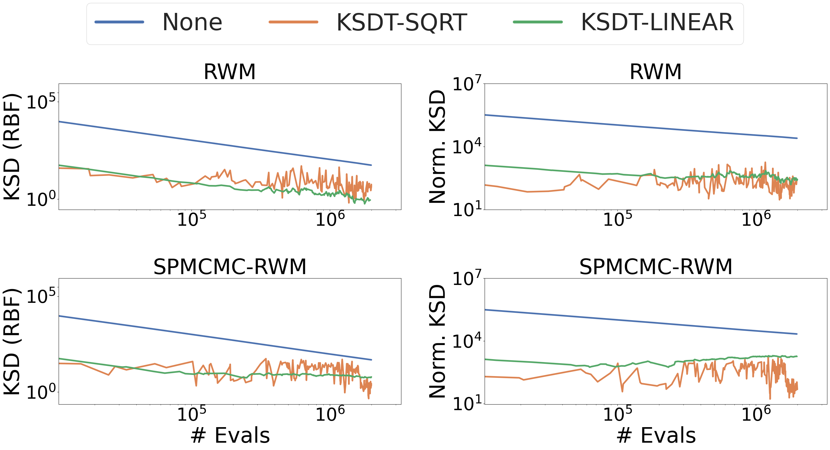
Figure 11: Goodwin problem, RBF base kernel. Comparison of un-thinned sample chains from the RWM and SPMCMC-RWM samplers with our thinning methods KSDT-SQRT and KSDT-LINEAR. Lower KSD and lower Normalized KSD indicate more accurate representations of the target distribution. Both axes are log-scale. Our methods outperform the baseline methods on both KSD and Normalized KSD.

7.2 Calcium Signalling Model

We report the results on a per-sampler basis when applying KSD thinning to the tempered RWM sampler with and without the SPMCMC update rule using either the RBF or IMQ kernels in Figures 12,13. In all cases the conclusions are similar to those we draw from Figure 4 in the main body. After accounting for model complexity (number of retained samples) with the Normalized KSD metric our methods outperform the baseline samplers. Our KSDT-LINEAR and KSDT-SQRT methods outperforms the baseline sampler more often than not on the (un-normalized) KSD metric as well.

Figure 12: Cardiac problem, IMQ base kernel. Comparison of un-thinned sample chains from the tempered RWM and SPMCMC-RWM samplers with our thinning methods KSDT-SQRT and KSDT-LINEAR. Lower KSD and lower Normalized KSD indicate more accurate representations of the target distribution. Both axes are log-scale. Our methods are competitive on KSD and outperform the baseline methods on Normalized KSD.

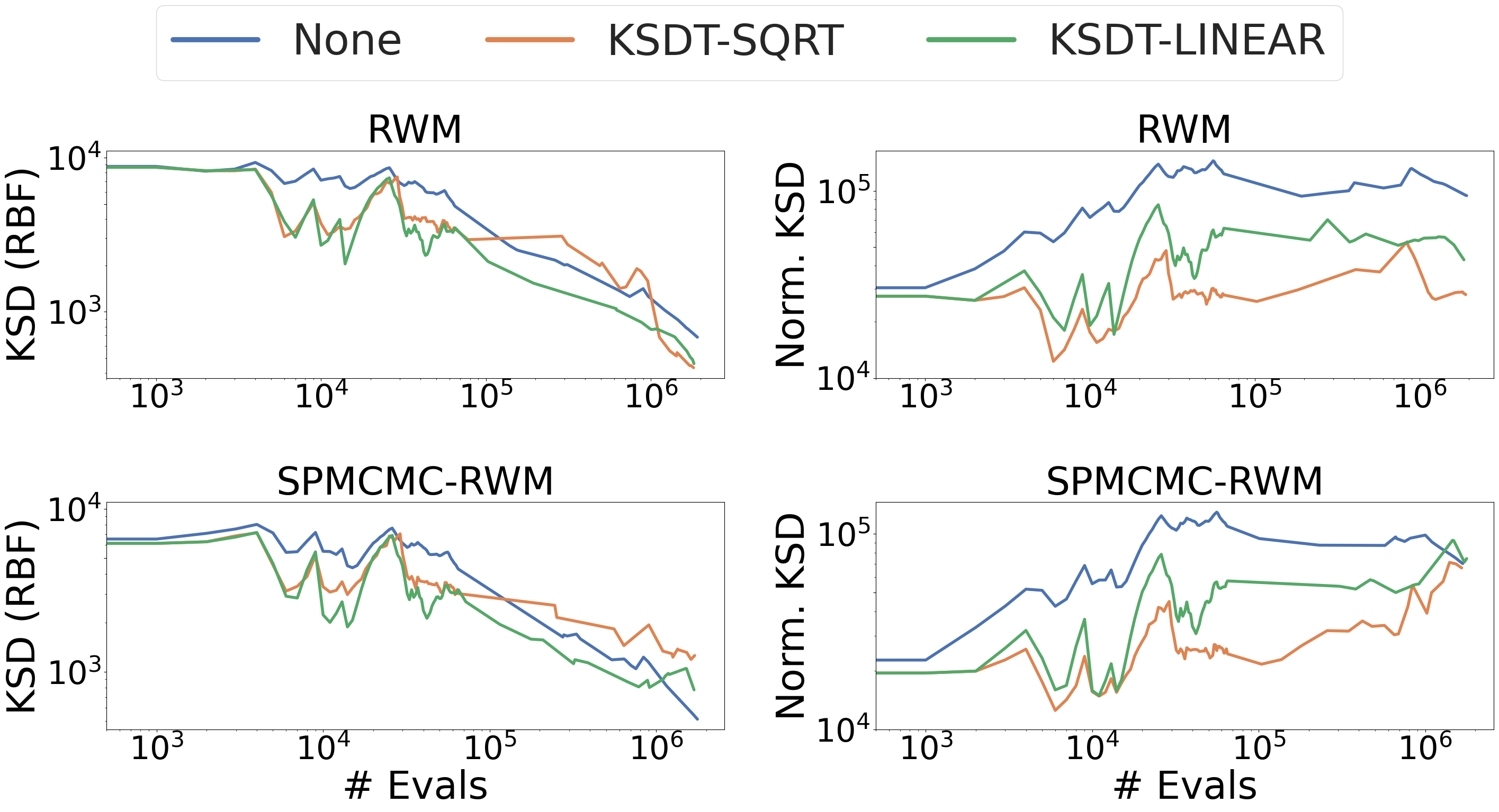
Figure 13: Cardiac problem, RBF base kernel. Comparison of un-thinned sample chains from the tempered RWM and SPMCMC-RWM samplers with our thinning methods KSDT-SQRT and KSDT-LINEAR. Lower KSD and lower Normalized KSD indicate more accurate representations of the target distribution. Both axes are log-scale. Our methods are competitive on KSD and outperform the baseline methods on Normalized KSD.

7.3 Bayesian Neural Network Subspace Sampling

In this appendix we provide additional results on accuracy and calibration as well as results using the RBF base kernel. No batch normalization or data augmentation is used as they do not admit Bayesian interpretations (Wenzel et al., 2020). In all experiments the hyper-parameters were optimized only for the ground truth MCMC chain. We set the SPMCMC parameter to $m=5$ and all methods perform 2000 SGLD steps. We measure the agreement, total variation, and the number of dictionary samples at steps $\{100,200,500,1000,2000\}$ for each task.

Curve Subspace

In order to construct the curve subspace we follow the procedure of (Izmailov et al., 2020b). First we pretrain two neural networks with Stochastic Weight Averaging (Izmailov et al., 2018). Next, given the weights $\mathbf{w}_{1},\mathbf{w}_{2}$ of two pretrained networks we initialize the curve midpoint $\mathbf{w}_{1/2}=\left(\mathbf{w}_{1}+\mathbf{w}_{2}\right)$ and define the piece-wise linear curve

$$\mathbf{w}_{t}=\begin{cases}\mathbf{w}_{1}+\frac{t}{0.5}\left(\mathbf{w}_{1/2}-\mathbf{w}_{1}\right)&\text{ if }0\leq t\leq 0.5\\ \mathbf{w}_{1/2}+\frac{t-0.5}{0.5}\left(\mathbf{w}_{2}-\mathbf{w}_{1/2}\right)&\text{ if }0.5<t\leq 1.0\end{cases}$$ (55)

where $t\in\left(0,1\right)$. To train the curve network, for each batch we sample $t\in(0,1)$ and backpropagate gradients only to $\mathbf{w}_{1/2}$. Finally, we define $\hat{\mathbf{w}}=(\mathbf{w}_{0}+\mathbf{w}_{1})/2$ as the “base point” and $\mathbf{v}_{1}=\mathbf{w}_{0}-\hat{\mathbf{w}}$ and $\mathbf{v}_{2}=\mathbf{w}_{1/2}-\hat{\mathbf{w}}$ as the subspace vectors. We perform sampling in the 2D subspace centered at $\hat{\mathbf{w}}$ and spanned by the vectors $\mathbf{v}_{1},\mathbf{v}_{2}$.

CIFAR-10 Classification

We present results for both total variation and ECE when using the RBF kernel for all KSD-based methods in Figure 14 demonstrate that our online thinning method outperforms both the baseline sampler and SPMCMC-based samplers on the agreement metric. We draw the same conclusion as the main body: improvement is mixed on the total variation metric, where our methods outperform existing methods in the low-sample regime, but have similar performance to existing methods once the model complexity is high. In Figures 15 and 16 we report results for accuracy and expected calibration error (ECE) using the RBF and IMQ kernels respectively. We observe that our thinning methods usually Pareto dominate the baseline methods on accuracy, and offer new points on the ECE Pareto frontier. We note that the goal of all methods is to match the predictive posterior distribution, not necessarily to achieve low accuracy. If the ground-truth predictive posterior has low accuracy and high ECE, then methods that perform best on the task of matching the posterior may have lower accuracy and higher ECE.

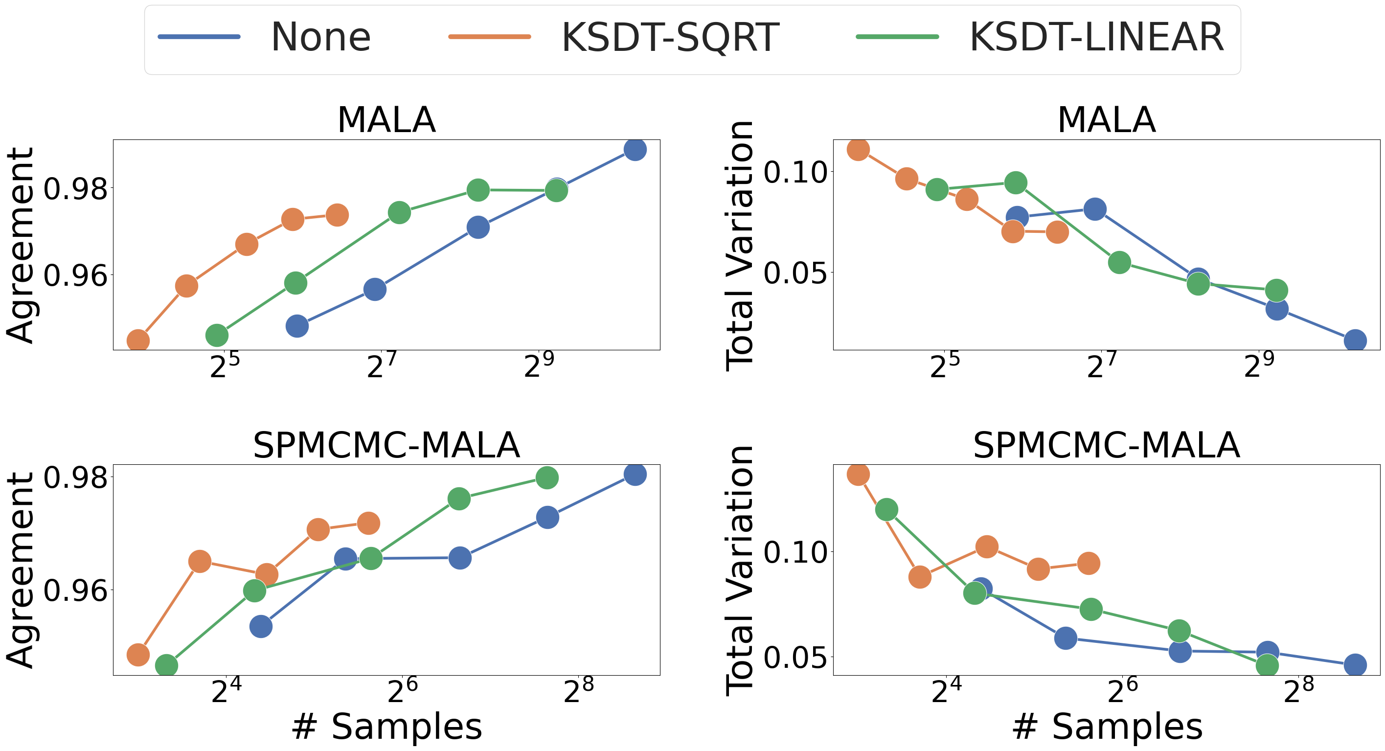
Figure 14: Agreement (left) and total variation (right) with the ground truth CIFAR-10 posterior predictive distribution. Higher Agreement and lower Total Variation indicate more accurate representation of the posterior predictive distribution. Color indicates thinning method (or baseline without thinning). The x-axis is log-scale. RBF base kernel. Our methods Pareto-dominate the baseline samplers on the Agreement metric and improve the Total Variation Pareto frontier in the low-sample regime.

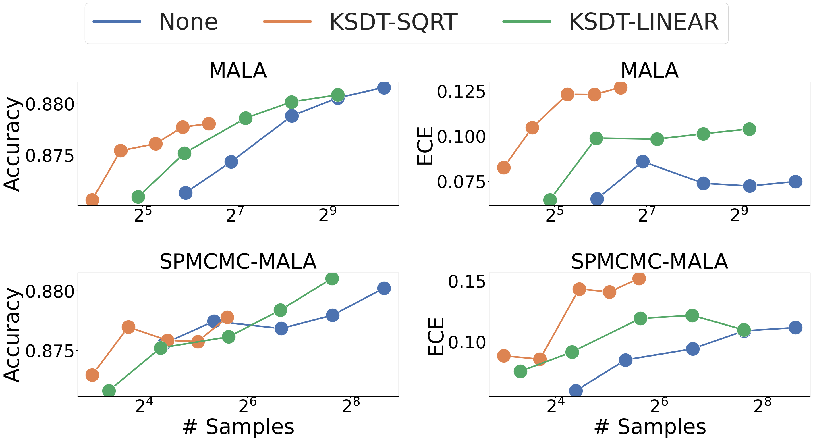
Figure 15: Accuracy (left) and Expected Calibration Error (right) on CIFAR-10 using the RBF base kernel. Higher Accuracy and lower ECE are better. Color indicates thinning method (or baseline without thinning). The x-axis is log-scale. Our methods Pareto-dominate the baseline samplers on accuracy and expand the low-sample Pareto frontier for ECE.

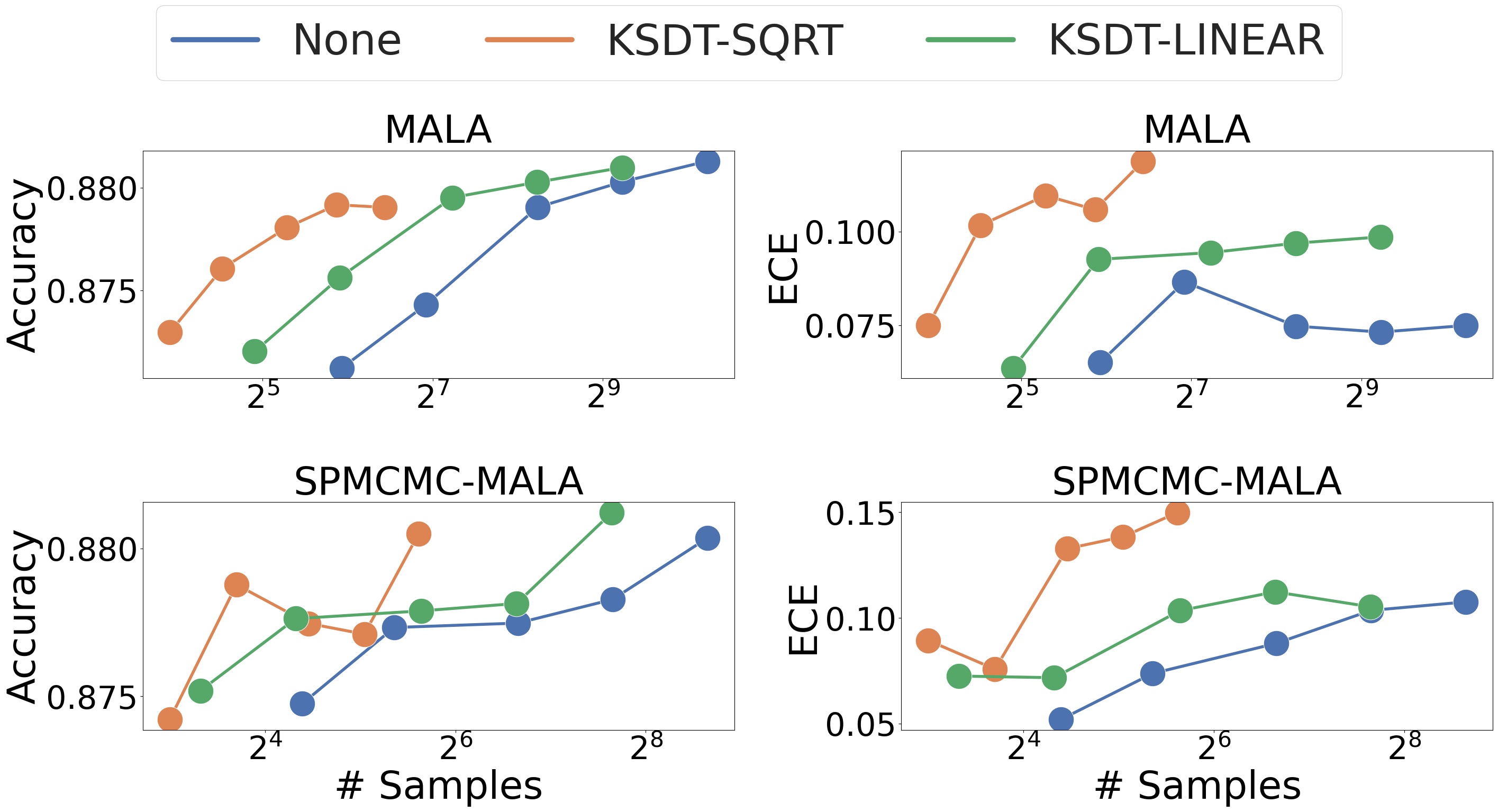
Figure 16: Accuracy (left) and Expected Calibration Error (right) on CIFAR-10 using the IMQ base kernel. Higher Accuracy and lower ECE are better. Color indicates thinning method (or baseline without thinning). The x-axis is log-scale. Our methods Pareto-dominate the baseline samplers on accuracy and expand the low-sample Pareto frontier for ECE.

IMDB Sentiment Prediction

We report results on both total variation and ECE when using the RBF kernel for all KSD-based methods in Figure 17. These results imply the same conclusion as the main body text IMQ kernel experiments: our online thinning method outperforms both the baseline sampler and SPMCMC-based samplers on the agreement metric. In Figures 18 and 19 we report results for accuracy and expected calibration error (ECE) using the RBF and IMQ kernels respectively. We observe that our thinning methods Pareto dominate the baseline methods on accuracy, and offer new points on the ECE Pareto frontier.

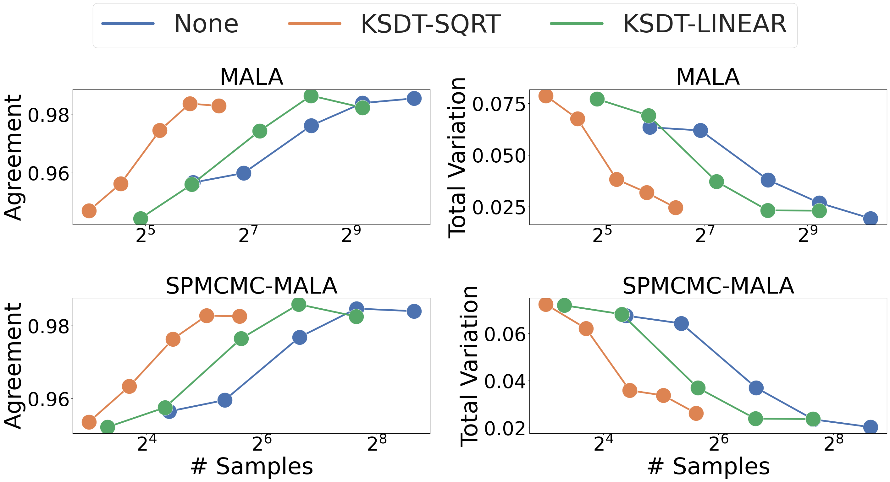
Figure 17: Agreement (left) and total variation (right) with the ground truth IMDB posterior predictive distribution. Higher Agreement and lower Total Variation indicate more accurate representation of the posterior predictive distribution. Color indicates thinning method (or baseline without thinning). The x-axis is log-scale. RBF base kernel. Our methods Pareto-dominate the baseline samplers on both the Agreement and Total Variation metrics.

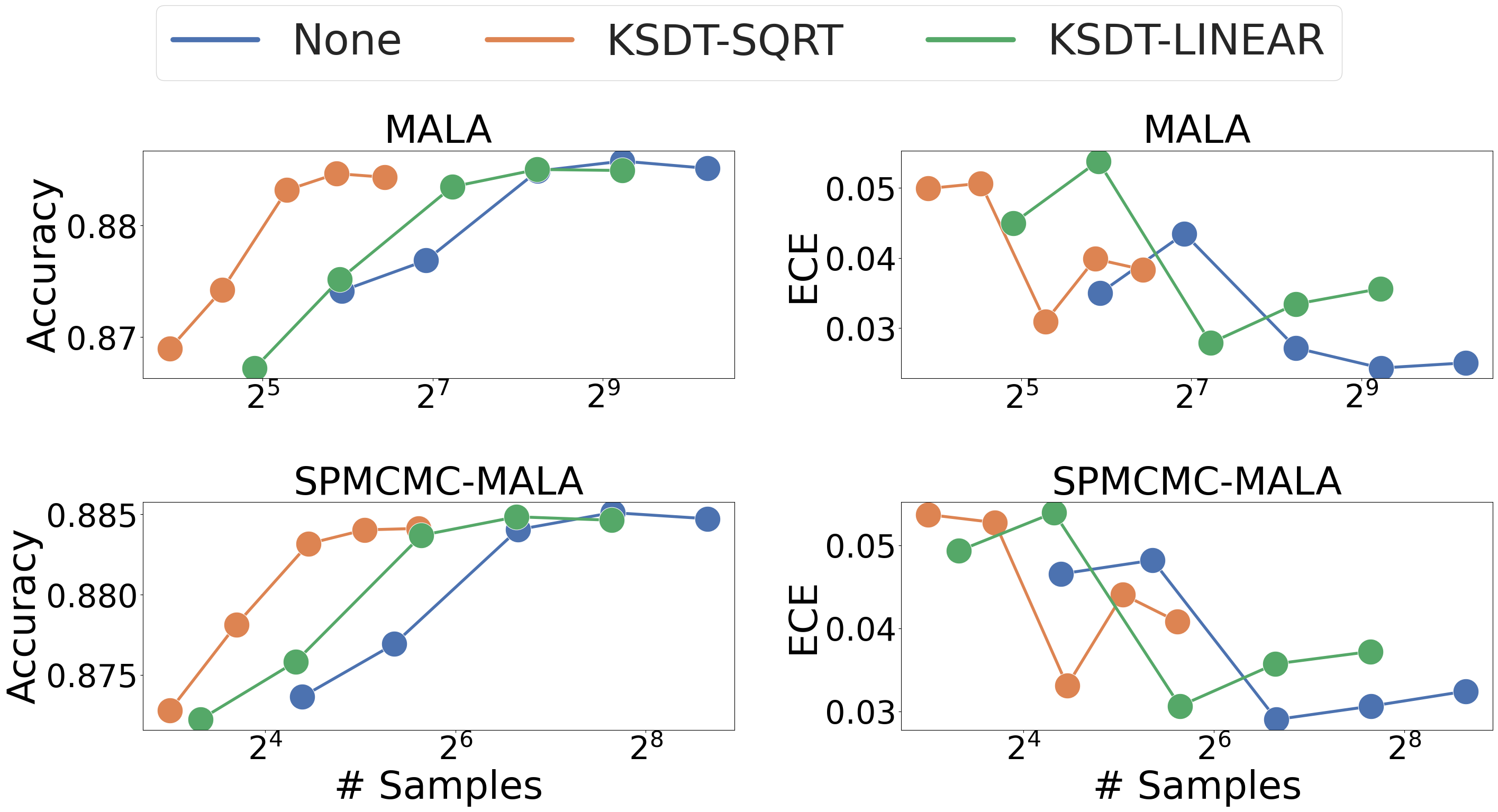
Figure 18: Accuracy (left) and Expected Calibration Error (right) on IMDB using the RBF base kernel. Higher Accuracy and lower ECE are better. Color indicates thinning method (or baseline without thinning). The x-axis is log-scale. Our methods Pareto-dominate the baseline samplers on accuracy and expand the low-sample Pareto frontier for ECE.

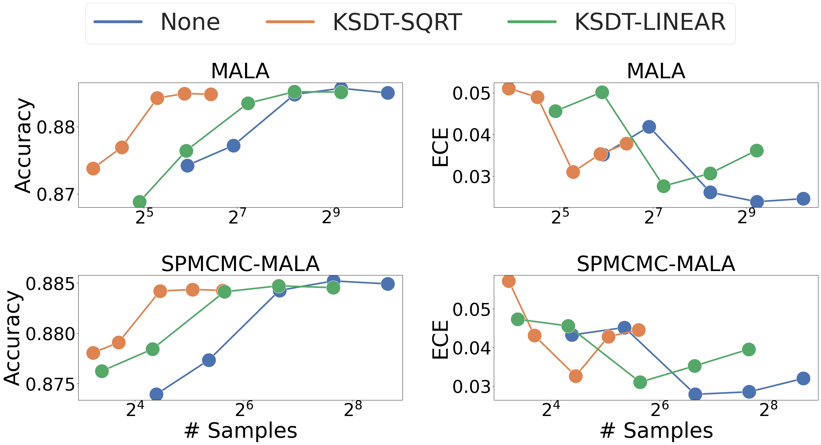
Figure 19: Accuracy (left) and Expected Calibration Error (right) on IMDB using the IMQ base kernel. Higher Accuracy and lower ECE are better. Color indicates thinning method (or baseline without thinning). The x-axis is log-scale. Our methods Pareto-dominate the baseline samplers on accuracy and expand the low-sample Pareto frontier for ECE.

7.4 Parameter Sensitivity

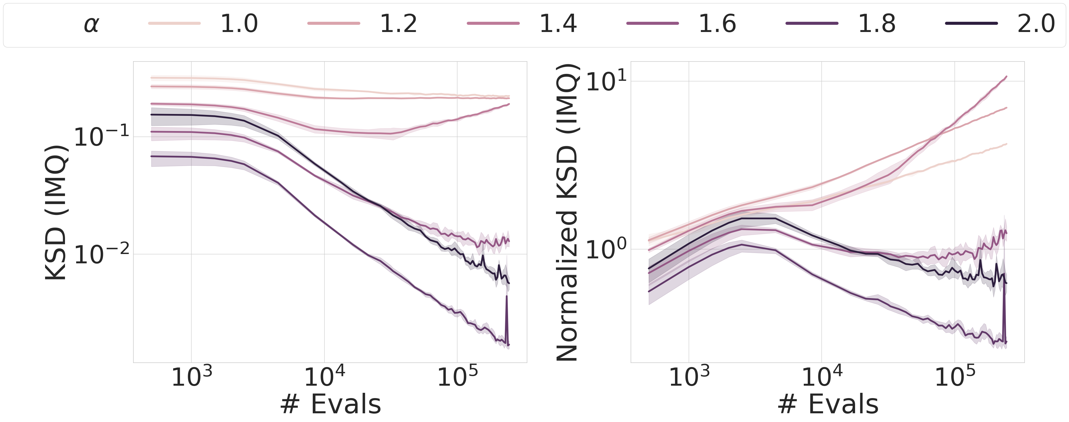
Figure 20: Sensitivity to dictionary growth rate parameter $\alpha$ on a bi-modal gaussian mixture problem. Lower KSD and lower Normalized KSD indicate more accurate representations of the target distribution. These results indicate that tuning the dictionary growth rate has potential to further improve our method.

We study the sensitivity of our thinning algorithm to the dictionary growth rate $f(i)\in o\left(\sqrt{i\log(i)}\right)$. We target an equally weighted bimodal Gaussian mixture distribution with means $\{(0,0),(1,1)\}$ and covariance $0.5*I_{2}$ for each mode. To decouple the sampler performance from our thinning algorithm we match the i.i.d. sampling setting of Theorem 1. We draw samples directly from the true distribution and apply the SPMCMC update rule with $m=5$. In Figure 20 we vary the exponent $\alpha$ with budget $f(t)=\sqrt{t^{\alpha}\log t}/2$. When $\alpha=2.0$ we use linear growth rate $f(t)=t/2$. We observe the results are sensitive to parameter tuning on this toy problem, and that the best setting for both KSD and normalized KSD is $\alpha=1.8$. Similar results for the RBF kernel are presented in Appendix Figure 21.

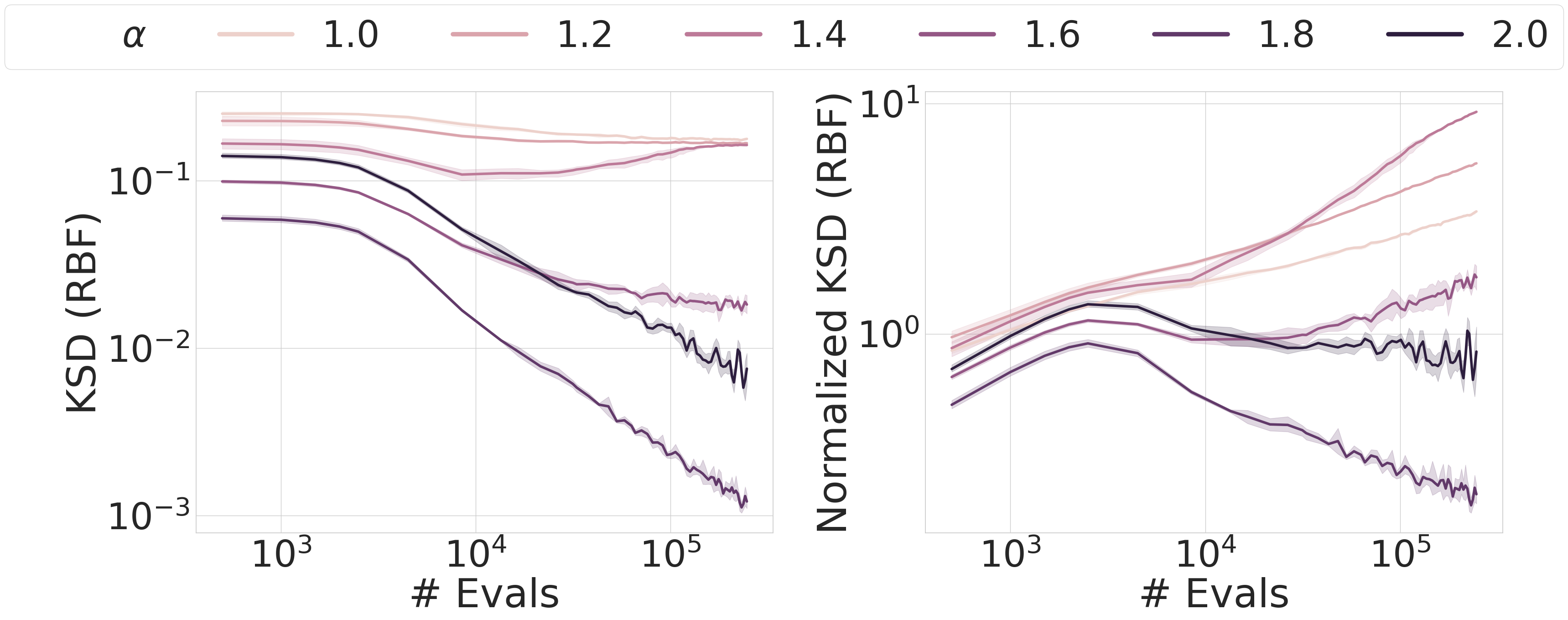
Figure 21: Sensitivity to dictionary growth rate parameter $\alpha$ on a bi-modal gaussian mixture problem using an RBF kernel. Lower KSD and lower Normalized KSD indicate more accurate representations of the target distribution. These results indicate that tuning the dictionary growth rate has potential to further improve our method.

In Figures 21 and 22 we repeat the same experiments with the RBF kernel instead of the IMQ kernel. In Figure 20 we vary the exponent $\alpha$ with budget $f(t)=\sqrt{t^{\alpha}\log t}/2$. When $\alpha=2.0$ we use linear growth rate $f(t)=t/2$. We observe the results are sensitive to parameter tuning on this toy problem, and that similar to the IMQ kernel experiment the best setting for both KSD and normalized KSD is $\alpha=1.8$.

7.5 Automatic Adaptation to Target Complexity

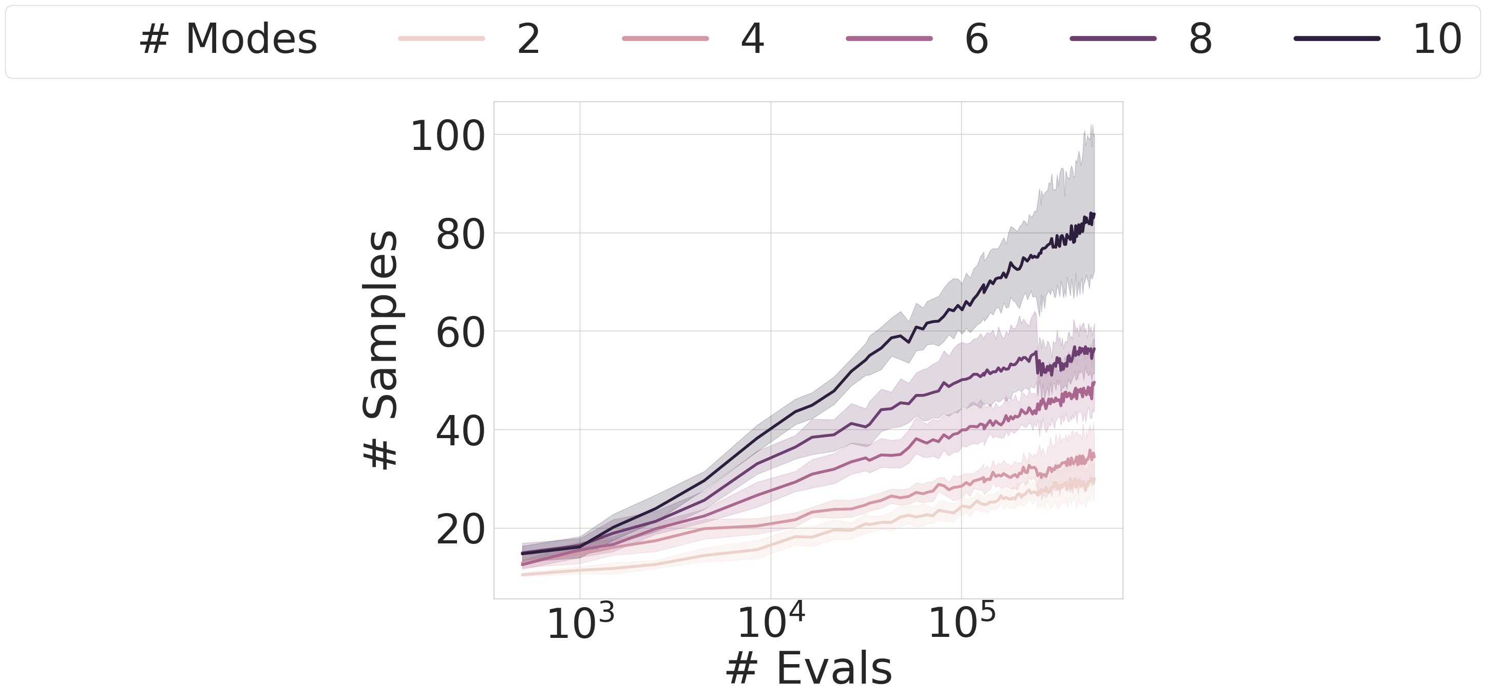
Figure 22: Base RBF kernel. As the number of modes of the Gaussian Mixture increases, our algorithm automatically adapts by increasing the number of samples.

In Figure 22 we observe that as the number of modes increases, so does the number of retained samples. This conclusion mirrors the IMQ kernel setting from Section 4.4.

8 Computational Complexity

This section addresses the per-step computational complexity of the problem

The evaluation of (9) does not require knowledge of the full symmetric kernel matrix $\mathbf{K}$ whose entries are $\mathbf{K}_{i,j}=k_{0}(\mathbf{z}_{i},\mathbf{z_{j}})$ for points $\mathbf{z}_{i}\in\mathbf{D}_{t-1}$. Assuming we maintain two vectors of size $|\mathbf{D}_{t}|$ (row sums and per-sample KSD contributions) we require $\mathcal{O}\left(|\mathbf{D}_{t-1}|\right)$ operations to evaluate (9). Evaluating the initial KSD to compute the thinning threshold $M$ requires summing the previous row sums with $\mathcal{O}\left(|\mathbf{D}_{t-1}|\right)$ operations. Computing a new row requires $|\mathbf{D}_{t-1}|$ evaluations of $k_{0}$. Updating previous row sums and KSD per-sample contributions requires $|\mathbf{D}_{t-1}|$ additions. Thinning requires searching a vector of size $|\mathbf{D}_{t-1}+1|$ for the maximum KSD contribution. A brute force search requires $\mathcal{O}\left(|\mathbf{D}_{t-1}|\right)$ operations. While thinning may occur more than once, we can amortize the cost of thinning across all time steps (since each sample can only be thinned once) to arrive at a worst case per-step complexity of $\mathcal{O}\left(t\right)$. In general, the thinning costs are orders of magnitude less expensive than the MCMC sampler costs.

References

- Berlinet & Thomas-Agnan (2011) Berlinet, A. and Thomas-Agnan, C. Reproducing kernel Hilbert spaces in probability and statistics. Springer Science & Business Media, 2011.
- Calderhead & Girolami (2009) Calderhead, B. and Girolami, M. Estimating bayes factors via thermodynamic integration and population mcmc. Computational Statistics & Data Analysis, 53(12):4028–4045, 2009.
- Chen et al. (2019a) Chen, W. Y., Barp, A., Briol, F.-X., Gorham, J., Girolami, M., Mackey, L., Oates, C., et al. Stein point markov chain monte carlo. arXiv preprint arXiv:1905.03673, 2019a.
- Chen et al. (2019b) Chen, W. Y., Barp, A., Briol, F.-X., Gorham, J., Girolami, M., Mackey, L., Oates, C., et al. Stein point markov chain monte carlo. arXiv preprint arXiv:1905.03673, 2019b.
- Constantine et al. (2016) Constantine, P. G., Kent, C., and Bui-Thanh, T. Accelerating markov chain monte carlo with active subspaces. SIAM Journal on Scientific Computing, 38(5):A2779–A2805, 2016.
- Cui et al. (2016) Cui, T., Law, K. J., and Marzouk, Y. M. Dimension-independent likelihood-informed mcmc. Journal of Computational Physics, 304:109–137, 2016.
- Detommaso et al. (2018) Detommaso, G., Cui, T., Spantini, A., Marzouk, Y., and Scheichl, R. A stein variational newton method. arXiv preprint arXiv:1806.03085, 2018.
- Dwivedi & Mackey (2021) Dwivedi, R. and Mackey, L. Kernel thinning. arXiv preprint arXiv:2105.05842, 2021.
- Goodwin (1965) Goodwin, B. C. Oscillatory behavior in enzymatic control processes. Advances in enzyme regulation, 3:425–437, 1965.
- Gorham & Mackey (2017) Gorham, J. and Mackey, L. Measuring sample quality with kernels. In Proceedings of the 34th International Conference on Machine Learning-Volume 70, pp. 1292–1301. JMLR. org, 2017.
- Hofmann et al. (2008) Hofmann, T., Schölkopf, B., and Smola, A. J. Kernel methods in machine learning. The annals of statistics, 36(3):1171–1220, 2008.
- Izmailov et al. (2018) Izmailov, P., Podoprikhin, D., Garipov, T., Vetrov, D., and Wilson, A. G. Averaging weights leads to wider optima and better generalization. arXiv preprint arXiv:1803.05407, 2018.
- Izmailov et al. (2020a) Izmailov, P., Maddox, W. J., Kirichenko, P., Garipov, T., Vetrov, D., and Wilson, A. G. Subspace inference for bayesian deep learning. In Uncertainty in Artificial Intelligence, pp. 1169–1179. PMLR, 2020a.
- Izmailov et al. (2020b) Izmailov, P., Maddox, W. J., Kirichenko, P., Garipov, T., Vetrov, D., and Wilson, A. G. Subspace inference for bayesian deep learning. In Uncertainty in Artificial Intelligence, pp. 1169–1179. PMLR, 2020b.
- Izmailov et al. (2021) Izmailov, P., Vikram, S., Hoffman, M. D., and Wilson, A. G. What are bayesian neural network posteriors really like? arXiv preprint arXiv:2104.14421, 2021.
- Koppel et al. (2017) Koppel, A., Warnell, G., Stump, E., and Ribeiro, A. Parsimonious online learning with kernels via sparse projections in function space. In 2017 IEEE International Conference on Acoustics, Speech and Signal Processing (ICASSP), pp. 4671–4675. IEEE, 2017.
- Koppel et al. (2020) Koppel, A., Pradhan, H., and Rajawat, K. Consistent online gaussian process regression without the sample complexity bottleneck. arXiv preprint arXiv:2004.11094, 2020.
- Korba et al. (2020) Korba, A., Salim, A., Arbel, M., Luise, G., and Gretton, A. A non-asymptotic analysis for stein variational gradient descent. Advances in Neural Information Processing Systems, 33, 2020.
- Lakshminarayanan et al. (2016) Lakshminarayanan, B., Pritzel, A., and Blundell, C. Simple and scalable predictive uncertainty estimation using deep ensembles. arXiv preprint arXiv:1612.01474, 2016.
- Link & Eaton (2012) Link, W. A. and Eaton, M. J. On thinning of chains in mcmc. Methods in ecology and evolution, 3(1):112–115, 2012.
- Liu et al. (2016) Liu, Q., Lee, J., and Jordan, M. A kernelized stein discrepancy for goodness-of-fit tests. In International conference on machine learning, pp. 276–284, 2016.
- Ma et al. (2015) Ma, Y.-A., Chen, T., and Fox, E. B. A complete recipe for stochastic gradient mcmc. arXiv preprint arXiv:1506.04696, 2015.
- Martin et al. (2012) Martin, J., Wilcox, L. C., Burstedde, C., and Ghattas, O. A stochastic newton mcmc method for large-scale statistical inverse problems with application to seismic inversion. SIAM Journal on Scientific Computing, 34(3):A1460–A1487, 2012.
- Neal (2012) Neal, R. M. Bayesian learning for neural networks, volume 118. Springer Science & Business Media, 2012.
- Paige et al. (2016) Paige, B., Sejdinovic, D., and Wood, F. D. Super-sampling with a reservoir. In UAI, volume 32, pp. 567–576, 2016.
- Peherstorfer et al. (2018) Peherstorfer, B., Willcox, K., and Gunzburger, M. Survey of multifidelity methods in uncertainty propagation, inference, and optimization. Siam Review, 60(3):550–591, 2018.
- Raftery & Lewis (1996) Raftery, A. E. and Lewis, S. M. Implementing mcmc. Markov chain Monte Carlo in practice, pp. 115–130, 1996.
- Riabiz et al. (2020) Riabiz, M., Chen, W., Cockayne, J., Swietach, P., Niederer, S. A., Mackey, L., Oates, C., et al. Optimal thinning of mcmc output. arXiv preprint arXiv:2005.03952, 2020.
- Roberts & Tweedie (1996) Roberts, G. O. and Tweedie, R. L. Exponential convergence of langevin distributions and their discrete approximations. Bernoulli, pp. 341–363, 1996.
- Seeger et al. (2003) Seeger, M. W., Williams, C. K., and Lawrence, N. D. Fast forward selection to speed up sparse gaussian process regression. In International Workshop on Artificial Intelligence and Statistics, pp. 254–261. PMLR, 2003.
- Snelson & Ghahramani (2005) Snelson, E. and Ghahramani, Z. Sparse gaussian processes using pseudo-inputs. Advances in Neural Information Processing Systems, 18:1257–1264, 2005.
- Sriperumbudur et al. (2010) Sriperumbudur, B. K., Gretton, A., Fukumizu, K., Schölkopf, B., and Lanckriet, G. R. Hilbert space embeddings and metrics on probability measures. The Journal of Machine Learning Research, 11:1517–1561, 2010.
- Stein (1972) Stein, C. A bound for the error in the normal approximation to the distribution of a sum of dependent random variables. In Proceedings of the sixth Berkeley symposium on mathematical statistics and probability, volume 2: Probability theory, pp. 583–602. University of California Press, 1972.
- Teymur et al. (2020) Teymur, O., Gorham, J., Riabiz, M., Oates, C., et al. Optimal quantisation of probability measures using maximum mean discrepancy. arXiv preprint arXiv:2010.07064, 2020.
- Wang et al. (2012) Wang, Z., Crammer, K., and Vucetic, S. Breaking the curse of kernelization: Budgeted stochastic gradient descent for large-scale svm training. Journal of Machine Learning Research, 13(100):3103–3131, 2012. URL http://jmlr.org/papers/v13/wang12b.html.
- Welling & Teh (2011) Welling, M. and Teh, Y. W. Bayesian learning via stochastic gradient langevin dynamics. In Proceedings of the 28th international conference on machine learning (ICML-11), pp. 681–688. Citeseer, 2011.
- Wenzel et al. (2020) Wenzel, F., Roth, K., Veeling, B. S., Swikatkowski, J., Tran, L., Mandt, S., Snoek, J., Salimans, T., Jenatton, R., and Nowozin, S. How good is the bayes posterior in deep neural networks really? arXiv preprint arXiv:2002.02405, 2020.
- Williams & Seeger (2001) Williams, C. and Seeger, M. Using the nyström method to speed up kernel machines. In Leen, T., Dietterich, T., and Tresp, V. (eds.), Advances in Neural Information Processing Systems, volume 13. MIT Press, 2001. URL https://proceedings.neurips.cc/paper/2000/file/19de10adbaa1b2ee13f77f679fa1483a-Paper.pdf.
- Williams & Rasmussen (2006) Williams, C. K. and Rasmussen, C. E. Gaussian processes for machine learning, volume 2. MIT press Cambridge, MA, 2006.