Alchemical geometry relaxation

Abstract

We propose to relax geometries throughout chemical compound space (CCS) using alchemical perturbation density functional theory (APDFT). APDFT refers to perturbation theory involving changes in nuclear charges within approximate solutions to Schrödinger’s equation. We give an analytical formula to calculate the mixed second order energy derivatives with respect to both, nuclear charges and nuclear positions (named ”alchemical force”), within the restricted Hartree-Fock case. We have implemented and studied the formula for its use in geometry relaxation of various reference and target molecules. We have also analysed the convergence of the alchemical force perturbation series, as well as basis set effects. Interpolating alchemically predicted energies, forces, and Hessian to a Morse potential yields more accurate geometries and equilibrium energies than when performing a standard Newton Raphson step. Our numerical predictions for small molecules including BF, CO, N2, CH₄, NH₃, H₂O, and HF yield mean absolute errors of of equilibrium energies and bond lengths smaller than 10 mHa and 0.01 Bohr for 4${}^{\text{th}}$ order APDFT predictions, respectively. Our alchemical geometry relaxation still preserves the combinatorial efficiency of APDFT: Based on a single coupled perturbed Hartree Fock derivative for benzene we provide numerical predictions of equilibrium energies and relaxed structures of all the 17 iso-electronic charge-netural BN-doped mutants with averaged absolute deviations of $\sim$27 mHa and $\sim$0.12 Bohr, respectively.

I Introduction

Chemical compound space is conceptually defined as the infinite set of all possible chemical compounds Kirkpatrick and Ellis (2004); Mullard (2017). Extensive knowledge of chemical compound space based on quantum mechanical calculations only is made extremely challenging by the unfathomably large number of molecules that have to be taken into consideration; in practical terms, only a small portion of it can be screened using standard computational methods. In order to improve our understanding of chemical compound space, as well as to enhance molecular design efforts, faster methods to scan chemical space are needed von Lilienfeld (2013); Freeze, Kelly, and Batista (2019). This can be achieved in two possible ways: either using an exact method at a low level of theory (cheap QM methods or force fields) or using an approximate method for estimating high-level theory calculations. Both quantum machine learning (QML) and alchemical perturbation density functional theory (APDFT) take advantage of data previously acquired, and generate new predictions using either interpolation (QML) or extrapolation (APDFT) techniques. QML Von Lilienfeld (2018); Rupp (2015) can be used effectively to predict several quantum properties von Lilienfeld, Müller, and Tkatchenko (2020); Rupp et al. (2012); Faber et al. (2017); Christensen, Faber, and von Lilienfeld (2019); Weinreich, Browning, and von Lilienfeld (2021); Pilania et al. (2013), recent works Bisbo and Hammer (2020); Lemm, von Rudorff, and von Lilienfeld (2021); Keith et al. (2021) succeeded in machine learning the optimized molecular geometries, but most QML methods do not predict directly geometrical structures.

APDFT von Rudorff and von Lilienfeld (2020a) is an alternative to QML for the rapid screening of chemical space. QML comes at the initial cost of securing a large training set, and this is not always available for the desired level of theory, the desired property of interest, or a relevant chemical subspace; in this regard, APDFT is more versatile because it requires the explicit QM calculation of only one reference molecule. From the reference molecule calculation and through the use of alchemical perturbations, it is possible to subsequently obtain estimates of molecular properties for a combinatorially large number of target molecules von Rudorff and von Lilienfeld (2020a). APDFT accuracy depends on the perturbation order and on the basis set choice Domenichini, von Rudorff, and von Lilienfeld (2020). If a high-quality calculation (e.g. CCSD) is used as reference, the error in third-order energy prediction can be smaller than the error made using a cheaper QM method such as HF and MP2. Domenichini, von Rudorff, and von Lilienfeld (2020); von Rudorff and von Lilienfeld (2020a)

Alchemical changes and derivatives were at first introduced as a way to rationalize energy differences between molecules.Wilson (1962); Politzer and Parr (1974); Levy (1978) Successive works showed that APDFT is also capable of predicting many other molecular properties, such as electron densities, dipole moments von Rudorff and von Lilienfeld (2020a), ionization potentials Von Lilienfeld and Tuckerman (2006); Marcon, von Lilienfeld, and Andrienko (2007), HOMO energy eigenvalues von Lilienfeld (2009), band structuresChang and von Lilienfeld (2018), deprotonation energiesvon Rudorff and von Lilienfeld (2020b); Muñoz et al. (2020). APDFT is particularly convenient if applied to highly symmetric systems where the explicit calculation of only a few derivatives (all the others can be obtained by symmetry operations) is required, e.g., in the BN-doping of polycyclic aromatic hydrocarbons.Balawender et al. (2013); Al-Hamdani, Michaelides, and von Lilienfeld (2017); Balawender et al. (2018a) Using pseudopotentials, quantum alchemy can also be applied to crystal structures Marzari, de Gironcoli, and Baroni (1994); Saitta, De Gironcoli, and Baroni (1998); Bellaiche, García, and Vanderbilt (2002); Sheppard, Henkelman, and von Lilienfeld (2010); Solovyeva and von Lilienfeld (2016); Chang and von Lilienfeld (2018), and can even suggest catalyst improvements Griego et al. (2020); Saravanan et al. (2017); Griego, Saravanan, and Keith (2019); Griego, Kitchin, and Keith (2021); Griego et al. (2021).

One of the major remaining challenges in APDFT is to include geometry relaxation as the equilibrium molecular structure changes from reference to target; this would constitute a huge improvement over fixed atoms ”vertical” predictions. To the best of our knowledge, only two papers Chang et al. (2016); von Lilienfeld (2009) have tried to predict equilibrium energies, applying APDFT to ”non-vertical” energy predictions (predicting energies for a perturbation that includes both changes in nuclear charges and in geometry).

In this paper we propose an alternative approach: we predict the geometry energy derivatives (gradients and Hessians) for the target molecule, and subsequently, use them to relax the geometry (see Fig.1).

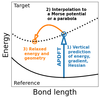
Figure 1: APDFT predictions of gradients and Hessians enable efficient geometry relaxation of target molecules. The predictive accuracy improves with Morse potential interpolation.

Alchemical forces are defined as the second-order mixed derivatives of the energy with respect to nuclear positions and nuclear charges ($\frac{\partial^{2}E}{\partial Z\partial R}$). Alchemical forces appear as non-diagonal terms in the generalized Hessian Fias, Chang, and von Lilienfeld (2019) ( the matrix that contains all the second derivatives of the energy with respect to nuclear charges, atoms’ positions, and electron number). Other off-diagonal terms correspond to nuclear Fukui functions De Proft, Liu, and Geerlings (1998); Baekelandt (1996); Balawender and Geerlings (2001); Laplaza et al. (2021) ($\frac{\partial^{2}E}{\partial N_{e}\partial R}$), alchemical Fukui functions Von Lilienfeld and Tuckerman (2006); Marcon, von Lilienfeld, and Andrienko (2007); Muñoz and Cárdenas (2017); Balawender et al. (2019); Gómez et al. (2021); Cárdenas, Heidar-Zadeh, and Ayers (2016) ($\frac{\partial^{2}E}{\partial N_{e}\partial Z}$)

Those functions have already been studied, while to the best of our knowledge no paper has yet carried out an in-depth analysis of alchemical forces. To study the predictive power and applications of alchemical predicted gradients and Hessians, we just consider the restricted Hartree Fock case. We think that an extension to UHF or DFT is possible, and some of the conclusions derived for RHF may also hold for other levels of theory.

In the first section of this paper, we will introduce the reader to the concept of APDFT, as well as to the Coupled Perturbed Hartree-Fock (CPHF) method used to calculate alchemical derivatives. We will derive an analytical formulation of RHF alchemical forces. In the second section we show that it is possible to compute higher-order derivatives through numerical differentiation and those derivatives can be used to predict geometrical gradients and Hessians for the target molecules, we also discuss how basis sets affect the accuracy of alchemical predictions of energy and geometry. In the results section, we give some examples of how to use the predicted gradients and Hessians to relax the geometry structures of the target molecules.

II Methods

II.1 Alchemical Perturbation Density Functional Theory

Within the Born Oppenheimer approximationBorn and Oppenheimer (1927), the non-degenerate electronic ground state wave function $\Psi_{0}(\mathbf{r};\mathbf{R},\mathbf{Z},N_{e})$ depends parametrically on the positions of the nuclei $\mathbf{R}$, the nuclear charges $\mathbf{Z}$, and the number of electrons $N_{e}$. The nuclear charge vector $\mathbf{Z}$ specifies the chemical composition of a given molecule, for real molecules $\mathbf{Z}$ can only have integer values, though from a theoretical point of view it is possible to extend the concept of atomic charge to any real number. It is thus possible to define a smooth path for $\mathbf{Z}$ coordinates that connects molecules of different chemical composition Von Lilienfeld and Tuckerman (2006). We call ”alchemical transmutation” the process of transforming one element into another for one or more atoms in a molecule. In order to connect a reference molecule R to a target molecule T we can define the alchemical coordinate $\lambda$ as a linear transformation of the nuclear charges from the reference $\mathbf{Z}^{\text{R}}=\mathbf{Z}(\lambda=0)$ to the target $\mathbf{Z}^{\text{T}}=\mathbf{Z}(\lambda=1)$.

$$\mathbf{Z}(\lambda) \equiv\mathbf{Z}^{\text{R}}+\lambda(\mathbf{Z}^{\text{T}}-\mathbf{Z}^{\text{R}})=\mathbf{Z}^{\text{R}}+\lambda\Delta\mathbf{Z}$$ (1)

The linear transformation of the nuclear charges corresponds also to a linear transformation of the electronic Hamiltonian and the nuclear-electron attraction operators $\hat{V}_{ne}$:

$$\hat{H}(\lambda) =\hat{H}^{R}+\lambda(\hat{H}^{T}-\hat{H}^{R})=\hat{H}^{R}+\lambda(\hat{V}_{ne}^{T}-\hat{V}_{ne}^{R})$$ (2)

$$\hat{H}(\lambda) =\hat{H}^{R}+\lambda\Delta\hat{V}_{ne}$$

For isoelectronic transmutations, the total electronic ground state energy of the molecule is continuous and differentiable in $\lambda$. von Lilienfeld (2009) From the energy of the reference molecule $E^{\text{R}}=E(\lambda=0)$ and its derivatives, we can express the energy of the target molecule $E^{\text{T}}=E(\lambda=1)$ through a Taylor series expansion, where $\Delta\lambda=1$ and where we assume convergence.

$$E^{\text{T}}=E^{\text{R}}+\sum_{n=1}^{\infty}{\frac{1}{n!}\left.\frac{\partial^{n}E(\lambda)}{\partial\lambda^{n}}\right|_{\lambda=0}}$$ (3)

Truncating the series in Eq.3 to a certain order will give an approximation of $E^{\text{T}}$. We call APDFTn prediction the approximation that includes all terms up to the n${}^{\textit{th}}$ order.

For a variational wave function, the first alchemical derivative of the electronic energy can be evaluated via the Hellmann-Feynman theorem Feynman (1939); von Lilienfeld (2009):

$$\left.\frac{\partial E}{\partial\lambda}\right|_{\lambda=0} =\bra{\psi_{\text{R}}}\hat{H}_{\text{T}}-\hat{H}_{\text{R}}\ket{\psi_{\text{R}}}$$ (4)

$$=\int_{\Omega}d\mathbf{r}\Delta V_{ne}(\mathbf{r})\rho_{\text{R}}(\mathbf{r})$$

For a monodeterminantal wave function (e.g. the solution of an Hartree Fock or a Kohn-Sham DFT calculation) the first alchemical derivative (Equation 4) can be rewritten as a contraction between the one electron density matrix $P$ of the reference molecule with the change in the nuclear-electron potential energy operator $\Delta V$:

$$\left.\frac{\partial E}{\partial\lambda}\right|_{\lambda=0} =\sum_{\mu\nu}P_{\mu\nu}\Delta V_{\mu\nu}$$ (5)

Higher order derivatives can be obtained via numerical differentiation or analytically using either Møller Plesset perturbation theory Chang et al. (2016) or a coupled perturbed approach (CPHF or CPKS-DFT) Lesiuk, Balawender, and Zachara (2012). The contribution of nuclear nuclear repulsion to the alchemical derivatives can be obtained analytically as the derivative of a classical charge distribution.

II.2 Coupled Perturbed Hartree Fock

Coupled perturbed methods are a powerful tool to calculate derivatives properties of a mono determinant wave function (HF,DFT). They represent the standard way to calculate polarization Cammi, Cossi, and Tomasi (1996); Caves and Karplus (1969); Dalgarno (1962) and can also be used for alchemical perturbations. Balawender et al. (2019, 2018a, 2013, 2018b)

The mathematical treatment to calculate the molecular response to an external electric field or to the electric field generated by the transmutation of one atom is indeed identical; here we would like to recall some theoretical aspects of the coupled perturbed Hartree Fock method.

In CPHF the first derivative of the coefficient’s matrix $C$ is written as a the product of $C$ and a unitary response matrix $U$:

$$\left(\frac{\partial C}{\partial\lambda}\right)=CU$$ (6)

From the orthogonality condition $C^{T}SC=I$ it is possible to show that $U$ must be skew symmetric.

$$\frac{\partial}{\partial\lambda}(C^{T}SC)=0$$ (7)

$$U^{T}(C^{T}SC)+(C^{T}SC)U=0$$

$$U=-U^{T}$$

Since $U$ acts as a rotation matrix, and since orbital rotations inside the occupied-occupied and the virtual-virtual blocks do not affect the total energy, we can choose the $o-o$ and the $v-v$ blocks of $U$ to be zero; keeping only the $o-v$ blocks of $U$ non zero. The derivative of the Roothaan equation $FC=SC\epsilon$ with respect to $\lambda$ becomes:

$$\frac{\partial F}{\partial\lambda}C+FCU=SCU\epsilon+SC\frac{\partial\epsilon}{\partial\lambda}\\$$ (8)

Multiplying from the left by $C^{T}$ and simplifying using the identities $C^{T}SC=I$ and $C^{T}FC=\epsilon$, leads to:

$$C^{T}\frac{\partial F}{\partial\lambda}C=U\epsilon-\epsilon U+\frac{\partial\epsilon}{\partial\lambda}$$ (9)

Since $\epsilon$ is a diagonal matrix and $U,U\epsilon,\epsilon U$ are zero on the diagonal blocks we can divide Equation 9 in two parts:

$$\left(C^{T}\frac{\partial F}{\partial\lambda}C\right)_{ia} =U_{ia}(\epsilon_{aa}-\epsilon_{ii})$$ (out of diagonal)

$$\left(C^{T}\frac{\partial F}{\partial\lambda}C\right)_{pq} =\frac{\partial\epsilon_{pq}}{\partial\lambda}$$ (on the diagonal)

We used the standard index notation for molecular orbitals, $i,j,k$ for occupied orbitals, $a,b,c$ for virtual orbitals, and $p,q,r$ for arbitrary orbitals. we will use Greek letters $\lambda,\mu,\nu,\sigma$ as indexes of atomic orbitals and capital letters $I,J,k$ as atoms’ indexes.

The partial derivative of the Fock matrix in Equation 9 contain the term $\partial V/\partial\lambda$, but also an implicit dependence on $U$ since $F$ depends on $C$. A detailed solution to the CPHF equations can be found in Refs.Pople et al. (1979); Cammi, Cossi, and Tomasi (1996); Lesiuk, Balawender, and Zachara (2012) After solving Eq. 9 derivatives of the one particle density matrix can be evaluated as:

$$\frac{\partial P_{\mu\nu}}{\partial\lambda} =\frac{\partial\left(C_{\mu i}C^{T}_{i\nu}\right)}{\partial\lambda}$$ (10)

$$=C_{\mu a}U_{ai}C_{i\nu}^{T}+C_{\mu i}U_{ia}^{T}C_{a\nu}^{T}$$

II.3 Second and third energy derivatives from atomic contributions

In APDFT any molecular property can be expressed as a function of the alchemical coordinate $\lambda$.
Explicating the dependence on the nuclear charges ($A(\lambda)=A\left(\mathbf{Z}(\lambda)\right)$), differentiation with respect to $\lambda$ can be performed using the chain rule:

$$\frac{\partial^{n}A}{\partial\lambda^{n}} =\left(\sum_{I}^{atoms}\frac{\partial Z_{I}}{\partial\lambda}\frac{\partial}{\partial Z_{I}}\right)^{n}A$$ (11)

$$\frac{\partial Z_{I}}{\partial\lambda} =Z_{I}^{T}-Z_{I}^{R}$$

The last equation comes directly from Eq.1 .

Solving the CPHF equation for any atom $I$ leads to the evaluation of a response matrix $U^{I}$ and of the first order derivatives ($\Delta V^{I},C^{I},F^{I},\epsilon^{I}$) of the operators with respect to the nuclear charge $Z_{I}$.

Consistently with the Wigner $2n+1$ rule, from these first order derivatives it is possible to evaluate the second and the third derivatives of the electronic energy:

$$\frac{\partial^{2}E}{\partial Z_{I}\partial Z_{J}}=4\sum_{a}\sum_{i}U^{I}_{ai}\Delta V^{J}_{ai}$$ (12)

$$\frac{\partial^{3}E}{\partial Z_{I}\partial Z_{J}\partial Z_{K}}=4[(IJK)+(JKI)+(KIJ)]$$ (13)

$$(IJK)=\sum_{i}^{occ.}\sum_{\mu\nu}F_{\mu\nu}^{I}C_{\mu i}^{J}C_{\nu i}^{K}-\sum_{ij}^{occ.}\sum_{\mu\nu}S_{\mu\nu}C_{\mu i}^{I}C_{\nu j}^{J}\epsilon^{K}_{ij}$$

This formulation is particularly convenient for highly symmetrical systems, where many of the derivatives ${\partial A}/{\partial Z_{I}}$ are symmetrically equivalent. Only few explicit CPHF calculations are needed, while the number of possible targets grows combinatorially with the size of the system.

II.4 Basis set energy correction

We pointed out in a previous paper Domenichini, von Rudorff, and von Lilienfeld (2020) that neglecting the derivatives of the basis set coefficients with respect to nuclear charges, i.e. calculating alchemical derivatives using the basis set of the reference molecule only, the alchemical series converges to the energy of the target molecule with the basis set of the reference ($E^{\text{T[R]}}$). The difference between this energy and the true target energy was named (alchemical) basis set error: $\Delta E_{\textrm{BS}}:=E^{\text{T[R]}}-E^{\text{T[T]}}$.
In the same paper we proposed a correction to the basis set error that can be added to any order APDFT energy prediction. The correction decomposes the total basis set error into a sum of individual atom contributions calculated from isolated atoms.

$$\Delta E_{\text{BS}}^{correction}:=\sum_{I}^{atoms}E^{\text{T[T]}}_{I}-E^{\text{T[R]}}_{I}$$ (14)

It is worth to mention the existence of the universal Gaussian basis set (UGBS)de Castro and Jorge (1998), an uncontracted basis set where all elements share the same basis sets exponents, thus there is no difference between reference and target basis sets.

II.5 Alchemical forces

Alchemical forces are the mixed derivatives of the energy with respect to both nuclear charges and nuclear positions Fias, Chang, and von Lilienfeld (2019). Alchemical forces can be computed analytically either by differentiating the alchemical potential with respect to the nuclear coordinates or differentiating the geometrical gradient with respect to the nuclear charges. In accordance with Schwarz’s theorem both methods are valid and will be presented below.

II.5.1 First formulation

Differentiating the first alchemical derivative of the electronic energy (Eq.5) with respect to the nuclear coordinates $\mathbf{R}_{I}$ of the atom $I$ leads to:

$$\frac{\partial}{\partial\mathbf{R}_{I}}\left(P\Delta V^{ne}\right)=\frac{\partial P}{\partial\mathbf{R}_{I}}\Delta V+P\frac{\partial\Delta V}{\partial\mathbf{R}_{I}}$$ (15)

where:

$$\frac{\partial\Delta V}{\partial\mathbf{R}_{I}}=\frac{\partial V}{\partial\mathbf{R}_{I}}\frac{\partial Z_{I}}{\partial\lambda}$$ (16)

The derivative of the one electron density matrix $\frac{\partial P}{\partial R}$ can be obtained through a CPHF calculation, independently for each molecular coordinate $R$, i.e. three times the number of atoms, for this reason we think is more convenient following the other approach.

II.5.2 Second formulation

Differentiating the geometrical gradient expression with respect to the nuclear charge of an atom ($Z_{I}$) requires only one density derivative $\frac{\partial P}{\partial Z_{I}}$, which is also needed for APDFT3 energy predictions.

The first derivative of the energy with respect to one nuclear Cartesian coordinate $R$ is: Pople et al. (1979)

$$\frac{\partial E}{\partial R} =\sum_{\mu\nu}P_{\mu\nu}\frac{\partial H_{\mu\nu}^{(1)}}{\partial R}$$ (17)

$$+\frac{1}{2}\sum_{\mu\nu\lambda\sigma}P_{\mu\nu}P_{\lambda\sigma}\frac{\partial}{\partial R}(\mu\lambda||\nu\sigma)$$

$$-\sum_{\mu\nu}W_{\mu\nu}\frac{\partial S_{\mu\nu}}{\partial R}$$

Where $H_{\mu\nu}^{(1)}$ is the mono electronic part of the Hamiltonian,$(\mu\lambda||\nu\sigma)$ is the sum of the bielectronic Coulomb and Exchange integrals, and $W$ is the energy weighted density matrix:

$$(\mu\lambda||\nu\sigma)\coloneqq \bra{\phi_{\mu}(\mathbf{r}_{1})\phi_{\lambda}(\mathbf{r}_{2})}\frac{1}{|\mathbf{r}_{1}-\mathbf{r}_{2}|}\ket{\phi_{\nu}(\mathbf{r}_{1})\phi_{\sigma}(\mathbf{r}_{2})}-$$ (18)

$$\frac{1}{2} \bra{\phi_{\mu}(\mathbf{r}_{1})\phi_{\lambda}(\mathbf{r}_{2})}\frac{1}{|\mathbf{r}_{1}-\mathbf{r}_{2}|}\ket{\phi_{\nu}(\mathbf{r}_{1})\phi_{\sigma}(\mathbf{r}_{2})}$$

$$W_{\mu\nu}\coloneqq \sum_{i}^{occ.}\epsilon_{i}C_{\mu i}C_{\nu i}^{T}$$

Eq.17 is composed of three terms, and we need to differentiate all of them with respect to the nuclear charge $Z_{I}$ of a given atom $I$.

For the first term of Eq.17:

$$\frac{\partial}{\partial Z_{I}}\left(P\frac{\partial H^{(1)}}{\partial R}\right)=\frac{\partial P}{\partial Z_{I}}\frac{\partial H^{(1)}}{\partial R}+P\frac{\partial^{2}H^{(1)}}{\partial Z_{I}\partial R}$$ (19)

The mono electronic Hamiltonian $H^{(1)}$ is composed of two parts: the kinetic energy operator $T$, which is independent of $Z_{I}$, and the nuclear electron potential $V$.

$$\frac{\partial^{2}H^{(1)}}{\partial Z_{I}\partial R} =\frac{\partial^{2}(T+V)}{\partial R\partial Z_{I}}=\frac{\partial}{\partial R}\frac{\partial V_{\mu\nu}}{\partial Z_{I}}$$ (20)

$$=\frac{\partial}{\partial R}\frac{\partial}{\partial Z_{I}}\sum_{J}^{atoms}\bra{\phi_{\mu}(\mathbf{r})}\frac{Z_{J}}{|\mathbf{R}_{J}-\mathbf{r}|}\ket{\phi_{\nu}(\mathbf{r})}$$

$$=\frac{\partial}{\partial R}\bra{\phi_{\mu}(\mathbf{r})}\frac{1}{|\mathbf{R}_{I}-\mathbf{r}|}\ket{\phi_{\nu}(\mathbf{r})}$$

The mixed derivative of the one electron Hamiltonian (Eq.20) is only non zero if the coordinate $R$ is referred to the position of atom $I$.

For the second term of Eq.17:

$$\frac{\partial}{\partial Z_{I}}(P_{\mu\nu}P_{\lambda\sigma}\frac{\partial}{\partial R}(\mu\lambda||\nu\sigma))=$$ (21)

$$P_{\mu\nu}\frac{\partial P_{\lambda\sigma}}{\partial Z_{I}}\frac{\partial}{\partial R}(\mu\lambda||\nu\sigma)+$$

$$\frac{\partial P_{\mu\nu}}{\partial Z_{I}}P_{\lambda\sigma}\frac{\partial}{\partial R}(\mu\lambda||\nu\sigma)$$

Differentiating the third term of Eq.17 yields:

$$\frac{\partial}{\partial Z_{I}}\left(W\frac{\partial S}{\partial R}\right)=\frac{\partial W}{\partial Z_{I}}\frac{\partial S}{\partial R}$$ (22)

The derivative of $W$ can be obtained from Equation 18 using the response matrix $U$ and the derivatives of the MO energies $\partial\epsilon/\partial Z_{I}$ from the solution of the CPHF equation (Eq.9):

$$\frac{\partial W}{\partial Z_{I}}=\sum_{i}^{occ.}\left(\epsilon_{i}(CU)_{\mu i}C_{\nu i}^{T}+\epsilon_{i}C_{\mu i}(CU)^{T}_{\nu i}+\frac{\partial\epsilon_{i}}{\partial Z_{I}}C_{\mu i}C_{\nu i}^{T}\right)$$ (23)

Collecting together all terms, the electronic part of the alchemical force at a RHF level of theory can than be expressed as follows:

$$\frac{\partial^{2}E}{\partial R\partial Z_{I}} =\frac{\partial P}{\partial Z_{I}}\frac{\partial H^{(1)}}{\partial R}+P\frac{\partial^{2}H^{(1)}}{\partial Z_{I}\partial R}$$ (24)

$$+\frac{\partial P_{\mu\nu}}{\partial Z_{I}}P_{\lambda\sigma}\frac{\partial}{\partial R}(\mu\lambda||\nu\sigma)$$

$$-\sum_{\mu\nu}\frac{\partial W_{\mu\nu}}{\partial Z_{I}}\frac{\partial S_{\mu\nu}}{\partial R}$$

II.5.3 Nuclear-nuclear contribution

The nuclear nuclear contribution to the alchemical force can be evaluated analytically as derivatives of an electrostatic charge distribution:

$$\frac{\partial^{2}E_{NN}}{\partial Z_{J}\partial\mathbf{R}_{I}}=\frac{Z_{I}(\mathbf{R}_{I}-\mathbf{R}_{J})}{|\mathbf{R}_{I}-\mathbf{R}_{J}|^{3}}(1-\delta_{IJ})+\sum_{Q}^{Q\neq I}\frac{Z_{Q}(\mathbf{R}_{I}-\mathbf{R}_{Q})}{|\mathbf{R}_{I}-\mathbf{R}_{Q}|^{3}}\ \delta_{IJ}$$ (25)

III Numerical Results

III.1 Computational details

All through our work we used a locally modified version of PySCF Sun et al. (2017) in which we implemented subroutines for the analytical alchemical derivatives (Eqs. 5, 12, 13), as well as the alchemical force (Eqs. 24,25). If not specified differently will be used the pcX-2 basis setAmbroise and Jensen (2019) for second row elements in conjunction with pc-2 basis set for hydrogen atoms. Basis sets’ coefficients and exponents were obtained from Basis Set Exchange Pritchard et al. (2019); Feller (1996); Schuchardt et al. (2007). Geometrical optimization in redundant internal coordinates was performed using a locally modified version of PyBerny Hermann (2020), where we included the transformation of the geometrical Hessian from Cartesian to internal coordinates. Root mean square deviations of atomic positions were evaluated using the program ”RMSD” Kromann (2021) implementing the Kabsch algorithm Kabsch (1976). Molecular sketch of benzene’s B-N mutants were plotted using RDKit. rdk (2013); Landrum (2013); Kim and Kim (2015) All Python code used in this work is made available, free of charge on a Zenodo repository. Domenichini (2021)

III.2 Convergence of gradients and Hessian series

Geometrical gradients and geometrical Hessians can be expanded as an alchemical series resulting into alchemical predictions of gradients and Hessians of the target molecules. The first alchemical prediction of the gradient is the alchemical force (Eqs.24,25).

Higher order derivatives of the gradient can be obtained through numerical differentiation of the alchemical force, while differentiation of the geometrical Hessian was only computed numerically. Derivatives were performed via a central finite difference stencil of 7 points equispaced by $\Delta\lambda=0.1$.

As a test case we choose to analyse the bond stretching of some diatomic molecules and the stretching of a C-H bond in a methane molecule, the results are plotted in Figure 2.

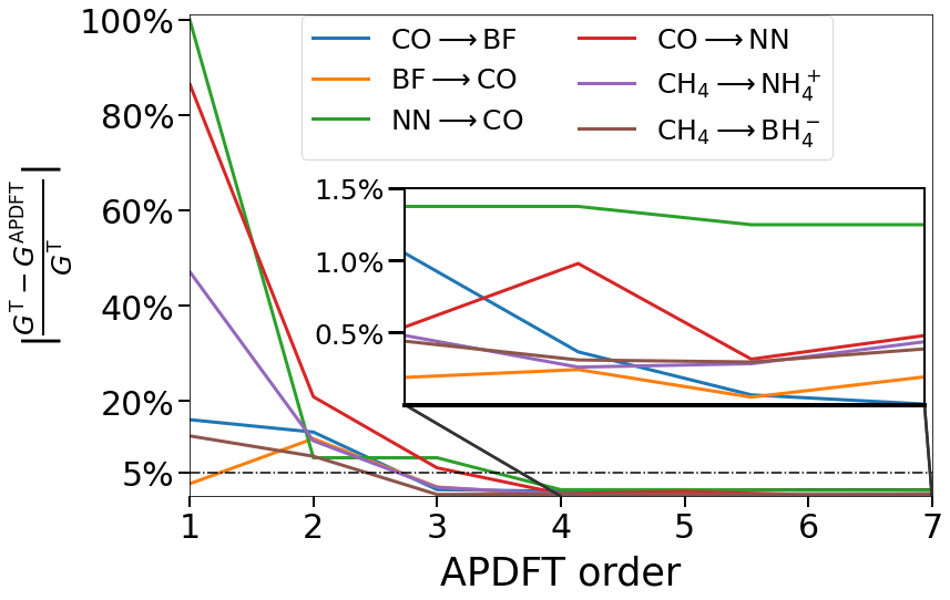
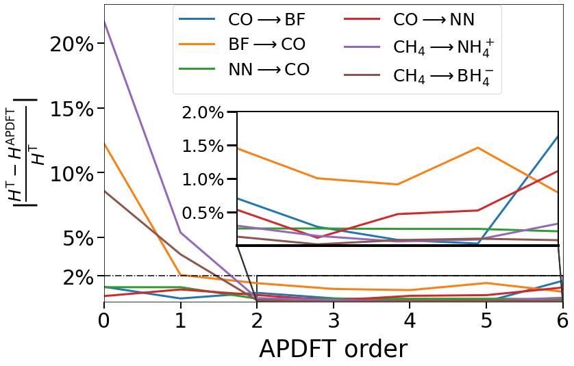
Figure 2: Decreasing error for APDFT predictions of geometrical gradients (TOP) and Hessians (BOTTOM) as perturbation order increases. Legends indicate respective colors for ”Ref. $\rightarrow$ Targ.” molecules. Inset shows convergence to less than 1.5%.

The zeroth order gradient prediction is just the gradient of the reference, which is zero in its geometrical minimum, this leads to a 100% prediction error for all molecules. Due to symmetry the alchemical force for the transmutation $\text{N}_{2}\rightarrow$CO is zero, therefore the first order term does not improve the prediction. The inverse transmutation CO$\rightarrow$N₂ has also an high first order error which can be justified by similar reasons.

The third order prediction leads to an error of about 5%, while predictions of orders higher than 4 lead to an error which is in any case below 1.50%. Going above 5${}^{\text{th}}$ order does not necessarily increase accuracy, because of numerical errors.

Furthermore if the derivatives of the atomic orbitals are neglected the Taylor series converges to the gradient of the target calculated with the basis set of the reference. We can see this effect in the prediction of N${}_{2}\rightarrow$CO where the green line has an offset of approximately 1.3%.

For Hessians the 0${}^{\text{th}}$ order prediction, i.e. approximating the target Hessian with the reference’s one, have still a certain degree of accuracy. Additional terms increase the precision and going above second order will lead to an error below 2%. The best predictions were obtained at the third and fourth and order, while after the fifth order term the series diverge due to numerical errors in the calculation of the Hessians.

III.3 Relaxed basis set errors

In a previous paper Domenichini, von Rudorff, and von Lilienfeld (2020) we stated that one of the major sources of error in APDFT vertical energy predictions is the alchemical basis set error, explained in section II.4.

For the sake of this paper is of great interest to analyse the alchemical basis set error error, not only for vertical energy predictions but also for the predictions of energies and geometries of the target in its energy minimum ”relaxed errors” ($\Delta E^{\text{BS}}_{eq},\Delta R^{\text{BS}}_{eq}$).

$$\Delta E^{\text{BS}}_{eq}:=E^{\text{T[R]}}_{eq}-E^{\text{T[T]}}_{eq}$$ (26)

$$\Delta R^{\text{BS}}_{eq}:=R^{\text{T[R]}}_{eq}-R^{\text{T[T]}}_{eq}$$

In the simple cases of diatomic molecules (BF$\leftrightarrow$CO, CO$\leftrightarrow$N₂) at the RHF level of theory, we tested performances of some of the most commonly used the triple and quadruple $\zeta$ basis set. We compared the family of Karlsruhe def2-nZ Schäfer, Huber, and Ahlrichs (1994); Weigend, Furche, and Ahlrichs (2003), the Dunning and coworker’s correlation consistent polarized valence cc-pVnZ Thorn H. Dunning (1989) and polarized core and valence cc-pCVnZ Woon and Dunning (1995), the Jensen’s polarization consistent pc-n Jensen (2001, 2002, 2007) and their uncontracted variant optimized for X-ray spectroscopy pcX-n Ambroise and Jensen (2019).

Figure 3: Alchemical basis-set errors (see Eqs. 26) for energy (TOP) and geometry (BOTTOM) as a function of number of atomic basis-functions. Values correspond to averages for BF, CO, and N₂ (which have been assessed as Ref. and Targ. molecules for APDFT predictions in Fig. 2, and Tables I and II).

Figure 3 shows that $\Delta E^{\text{BS}}_{eq}$ decrease with the increase in the basis set size, this trend is approximately linear in the logarithmic plot for def2, cc-pCVnZ and pc-n basis sets.
Core polarization is important for the alchemical invariance of basis sets; the cc-pVnZ basis functions which are only polarized on the valence shell have a higher $\Delta E^{\text{BS}}_{eq}$ compared to other basis of equal size.
As a proof of this concept we created a new basis set combining the core basis functions (the orbitals with $s$ symmetry) of the cc-pCVQZ basis set with the valence and polarization orbitals of the smaller cc-pCVTZ; the orthonormality of this basis set labeled cc-pCV(sQ)TZ is guaranteed by spherical symmetry.

In Figure 3 we can compare $\Delta E^{\text{BS}}_{eq}$ for cc-pCVTZ and cc-pCV(sQ)TZ basis sets: passing from 6 to 8 s type orbitals per atoms is enough to reduce the error by about one order of magnitude.

The cc-pVTZ basis set has a large geometry error, that’s because the systems, in order to compensate for the high energy error, increase the orbital overlap between the atoms shortening the bond lengths. The other basis sets of the cc-pVnZ family (cc-pVQZ and cc-pV5Z) don’t suffer as much from this problem. $\Delta R^{\text{BS}}_{eq}$ is similar for cc-pCV(sQ)TZ and cc-pCVTZ, both basis set share the same valence and polarization functions. We can conclude that a good description of core and valence atomic orbitals is needed for accurate APDFT energies, while a good description in valence orbitals and the presence of polarization functions is required for accurate geometry predictions.

Best results in terms of accuracy per basis sets number were achieved both for energy and geometry by the polarization consistent pcX-2 and pcX-3 basis sets. Those are uncontracted basis sets whose coefficients are optimized for X-Ray spectroscopy. To describe effectively a core-ionization of an atom, the basis functions used should provide a balanced representation of both the ground and core-excited state, where the effective nuclear charge changes by roughly $+1$. The same requirement is also true for alchemy, where the true nuclear charges change by $\pm 1$. This is a case where the computational solution to one specific problem (x-rays spectroscopy) can also be used effectively in a completely different application (APDFT). Acknowledged these conclusions on basis sets, we will use for the rest of the article the pCX-2 basis set, and since the pcX-2 basis sets are defined only for second and third row elements, for hydrogens we will use the pc-2 basis set.

IV Applications to geometry relaxation

In section III.2 we showed how alchemical perturbation can be used to predict geometrical gradients and Hessians. Those gradients and Hessians can be used to relax the geometry of the target molecule in several ways. We would like to show in this section that a geometrical relaxation using the alchemical predicted gradients and Hessians it is possible and can be accurate depending on the APDFT order.

IV.1 Relaxation techniques

The simplest relaxation technique is a single step in the Newton-Raphson optimization method. The potential energy surface is approximated with a paraboloid; given a a set of Cartesian coordinates $\mathbf{x}$, a gradient $\mathbf{g}$ and a Hessian $H$, the optimization step and the relaxation energy are:

$$\Delta\mathbf{x}=-H^{(-1)}\mathbf{g}$$ (27)

$$\Delta E=-\frac{1}{2}\Delta\mathbf{x}H\Delta\mathbf{x}$$ (28)

A better representation for the monodimensional potential of a bond stretching was given by Morse Morse (1929):

$$V_{Morse}(R;D_{e},R_{e},a,V_{e})=D_{e}(1-e^{-a(R-R_{e})})^{2}+V_{e}$$ (29)

Morse potentials depend on four parameters: the bond dissociation energy $D_{e}$, the equilibrium distance $R_{e}$, the parameter $a$ which controls the width of the potential well, and $V_{e}=V(r_{e})$ the value of the energy at the minimum.

Knowing the energy, the first and second derivatives at a given point of the curve, we can match the number of parameters with the number conditions using an empirical value for the dissociation energy. This is legit because the the interpolated curves do not depend sensibly on $D_{e}$, and analogously to what is done in the UFF Rappe et al. (1992) we will approximate $D_{e}$ with the value of 100kCal/mol times the total bond order (for UFF this parameter is 80kCal/mol).

For molecules bigger than diatomics is still possible to introduce the Morse potential interpolation as a correction to a Newton-Raphson step.

Using internal coordinates $\mathbf{q}$, we calculated the correction treating every bond if $b$ if it were an independent coordinate:

$$\Delta\mathbf{q}_{b}^{Corr.}=\Delta\mathbf{q}_{b}^{Morse}(\mathbf{q}_{b},\mathbf{g}_{b},H_{bb},D_{e(b)})-(-\mathbf{g}_{b}/H_{bb})$$ (30)

The mixed terms between different coordinates are still calculated in the paraboloid (Newton Raphson) approximation.

The Morse potential correction affect also the energy:

$$\Delta E^{Corr.}= -\frac{1}{2}\Delta\mathbf{q}^{T}H\Delta\mathbf{q}\$$ (31)

$$+\sum_{b}(\Delta E^{Morse}_{b}+\frac{1}{2}H_{bb}(\Delta\mathbf{q}_{b}^{Morse})^{2})$$

A more in detail discussion of the Morse potential interpolation is given in the supplementary materials of this paper.

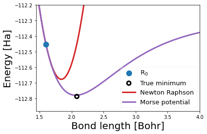
Figure 4: Morse interpolation improves geometry relaxation as exemplified for CO: Interpolating Hartree-Fock energies, gradients and Hessians at R₀ to Morse potential and parabola (Newton Raphson step) affords purple and red potentials, respectively.

Taking as an example the dissociation of CO, shown in figure 4, we can see that the quadratic approximation leads to a poor result when the starting point is far from the minimum. Since the geometries of reference and target are usually substantially different, this condition occurs quite often in alchemical relaxation.

At the Morse potential describes the whole energy curve of bond dissociations better, and this can lead to a more accurate relaxation, if the gradient and the Hessian are predicted accurately.

IV.2 Diatomics

In the simple case of diatomic molecules we can derive some considerations regarding the accuracy of the alchemical relaxation at different perturbation order, and compare the relaxations obtained using Newton Raphson step and the Morse potential interpolation.

Tab.1 shows the results obtained with a NR step. In the predictions CO$\rightarrow$BF and N${}_{2}\rightarrow$BF the error in bond lengths is consistent, and a higher alchemical order does not give better results.

Furthermore in this method is neglected the dependence of Hessian on the geometry, the different geometries of reference and target lead to a huge error in the prediction of harmonic vibrational frequencies.

Ref.	Targ.	APDFT	Req [Bohr]	$E$[Ha.]	$\omega_{0}$ [cm-1]
Newton Raphson optimization
N2	BF	2	2.290	-124.2586	2676
N2	BF	4	2.221	-124.1884	2678
CO	BF	2	2.285	-124.1862	2402
CO	BF	3	2.262	-124.1598	2407
CO	BF	4	2.258	-124.1634	2410
True	BF	-	2.353	-124.1624	1507
BF	CO	2	1.793	-112.7944	1415
BF	CO	3	1.846	-112.8141	1418
BF	CO	4	1.864	-112.8121	1431
N2	CO	2	2.080	-112.7909	2740
N2	CO	4	2.076	-112.7855	2740
True	CO	-	2.083	-112.7866	2430
BF	N2	2	0.813	-109.4238	1244
BF	N2	3	1.375	-109.1547	1274
BF	N2	4	1.761	-109.0494	1490
CO	N2	2	1.989	-108.9803	2416
CO	N2	3	2.009	-108.9977	2411
CO	N2	4	2.005	-108.9933	2415
True	N2	-	2.014	-108.9891	2730
MAE	$\Delta Z\pm 1$	2	0.097	0.0111	634
MAE	$\Delta Z\pm 1$	3	0.084	0.0108	635
MAE	$\Delta Z\pm 1$	4	0.083	0.0080	632
Morse optimization
N2	BF	2	2.543	-124.2904	1233
N2	BF	4	2.369	-124.2033	1440
CO	BF	2	2.412	-124.1965	1379
CO	BF	3	2.364	-124.1674	1453
CO	BF	4	2.354	-124.1704	1471
True	BF	-	2.353	-124.1624	1507
BF	CO	2	2.096	-112.7580	2744
BF	CO	3	2.101	-112.7867	2589
BF	CO	4	2.104	-112.7868	2572
N2	CO	2	2.090	-112.7913	2389
N2	CO	4	2.084	-112.7858	2408
True	CO	-	2.083	-112.7866	2430
BF	N2	2	2.133	-108.7587	5082
BF	N2	3	2.084	-109.0103	3510
BF	N2	4	2.110	-109.0010	3130
CO	N2	2	2.005	-108.9794	2910
CO	N2	3	2.019	-108.9973	2785
CO	N2	4	2.017	-108.9929	2812
True	N2	-	2.014	-108.9891	2730
MAE	$\Delta Z\pm 1$	2	0.022	0.0192	166
MAE	$\Delta Z\pm 1$	3	0.011	0.0045	77
MAE	$\Delta Z\pm 1$	4	0.007	0.0032	70

Table 1: APDFT based predictions of equilibrium distances and energies and frequencies using a single step of the parabola Newton Raphson (TOP) and Morse potential (BOTTOM) optimization. ’True’ corresponds to Hartree-Fock SCF results.

Tab.1 shows that the Morse method performs better than Newton Raphson’s. The biggest errors were made in the predictions N${}_{2}\leftrightarrow$CO where is involved an alchemical change of $\Delta Z=\pm 2$. All the other predictions which have $\Delta Z=\pm 1$ have an error in the bond length prediction on average of 0.011 Bohr at third order which decreases to 0.007 Bohr at fourth order. The error in the energy is also very low, 4.5 mHa and 3.2 mHa for APDFT3 and APDFT4 predictions respectively. The error in the harmonic frequencies prediction is about 70 cm^-1; is not accurate, but it is indicative of the value of the frequency.

IV.3 Alchemical protonation and deprotonation

Figure 5: Subsequent alchemical couplings connect the entire iso-electronic series of second period elements’ hydrides (CH₄,NH₃,BH₂,HF) through successive alchemical deprotonation (to the right) and protonation (to the left).

Deprotonation and protonation energies are important quantities, because describe the changes in enthalpy within an acid-base reactions, and are needed in the calculation of the equilibrium constants p$K_{a}$ and p$K_{b}$. Atkins and De Paula (2006); Carvalho et al. (2021); Casasnovas et al. (2009) In this section, we demonstrate how APDFT can be used to predict protonation and deprotonation energies accurately. APDFT3 error for vertical deprotonation energies can be as small as 1.4 kcal/mol von Rudorff and von Lilienfeld (2020b); Muñoz et al. (2020); Chang et al. (2016); Flores-Moreno et al. , we would like to go beyond the fixed geometry approximation including the geometrical relaxation energy. More specifically, we exemplify our approach for the alchemical navigation of the iso-electronic 10 electron series of second row hydrides CH${}_{4}\rightarrow$NH${}_{3}\rightarrow$H₂O$\rightarrow$ HF,(see figure 5 for illustration). Moving from one molecule to a neighbouring one, within alchemical deprotonation (protonation) a hydrogen nucleus is alchemically annihilated (created) while the nuclear charge of the heavy atom is simultaneously increased (decreased).

The initial guess of the protonation site was chose on the electrostatic potential minimum of the reference molecule; in that position we placed a basis set for the hydrogen created.

We implemented a three point finite difference stencil ($\Delta\lambda=0.1$), combining numerical and analytical differentiation we obtained second order Hessian predictions, third order gradient prediction and fifth order energy prediction.

Combining numerical differentiation from a three points finite difference scheme ($\Delta\lambda=0.1$) with analytical differentiation (Eqs.12, 13, 24), we calculated second order predictions for the Hessian, third order prediction for the gradient and fifth order prediction for the energy.

Geometry relaxation was performed using the Morse potential interpolation (Eqs. 30, 31).

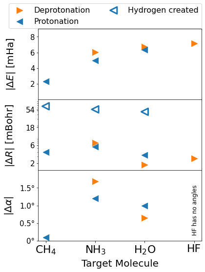
Figure 6: Absolute APDFT prediction errors of equilibrium energies (TOP), bond lengths (MID), and angle widths (BOTTOM) for the alchemical protonations and deprotonations (see Fig.5).

Figure 6 shows the errors in protonations and deprotonations. The average error on energy predictions is 7 mHa for deprotonation and 5 mHa for protonation; this error is already present in the vertical predictions, as such does not come from the geometrical relaxations.

Alchemical deprotonation can predict relaxed bond lengths accurately; results show a mean absolute error of 4 milli Bohr and in all cases, the error is lower than 10 milli Bohr, for protonations, the predicted bond length of the hydrogens that were already present in the reference molecule is different from the one of the alchemically created hydrogen.

The effect of alchemical perturbation is much higher on the created hydrogens, for this reason, the error in bond length predictions is 10 times higher than the error for hydrogens already present in the molecule, 56 and 4 milli Bohr respectively.

Angles are more flexible coordinates than bonds, therefore the prediction error of about 1^∘ is quite substantial, an exception is the prediction NH${}_{3}\rightarrow$ CH₄ where the smaller error might be due to a stiffer energy potential.

IV.4 B-N Doping of Benzene

Figure 7: A single APDFT3 reference calculation for benzene affords equilibrium energy predictions for all seventeen possible iso-electronic charge-neutral B-N doped mutants at Hartree-Fock level of theory.

APDFT is efficient in predicting properties for multiple targets from a few derivatives when symmetric systems are chosen as reference. An appealing application is the B-N doping of aromatic hydrocarbons such as coronenes, fullerenes, or graphene. Balawender et al. (2013); Fias, Chang, and von Lilienfeld (2019); Al-Hamdani, Michaelides, and von Lilienfeld (2017); Balawender et al. (2018a)

Here, we show that is possible to obtain approximate equilibrium energies and relaxed structures for all the 17 B-N doped mutants shown in Fig.7 through the explicit calculation of just one CPHF derivative for benzene. The CPHF response matrix $U$ can be obtained for all atoms via symmetry operations, in particular, we rotated the $U$ matrix around the symmetry axis of the molecule using the Wigner D-matrix Wigner (1931). Energy prediction up to third-order can be obtained using Eqs.5, 12, 13, the same CPHF derivatives can be reused to calculate the alchemical force in Eq.24. This is sufficient to give a first-order prediction of the geometrical gradient for all 17 target molecules. The targets’ Hessians were approximated at the zeroth order with the Hessian of the reference. As shown in Fig.2 this approximation has an error of approximately 20% for the isolectronic hydride series, which can still lead to qualitative improvements. In this case, the geometrical relaxation was performed using a Newton Raphson step and not Morse, because it is less sensible to errors in gradient and Hessian. We measure geometry prediction errors through the root mean square deviation from the true target molecules’ minima (RMSDKabsch (1976)). It is important to remark on the energy ordering of the mutants. Every B-N substitution corresponds to a decrease in energy of about 3 Hartree, therefore stoichiometry is the dominating dimension. Among constitutional isomers, energy ordering depends on the relative positions of B and N; for mono doped mutants, the least stable is the one with B and N in meta position, followed by the trans and the ortho isomers. This ordering is analogous to the reactivity in electrophilic-nucleophilic aromatic substitutions Bunnett and Zahler (1951). In fact, after a B-N doping of benzene, the electronic charge shifts from the boron atom to the nitrogen; in this context nitrogen atoms act as Lewis acids (electrophiles) and borons as Lewis bases (nucleophiles). Robles et al. (2018); Ayers, Anderson, and Bartolotti (2005) We note, however, that these trends change upon removal of the nuclear repulsion terms which do not affect the electronics. The predicted energy ordering is the same, both for the vertical and the relaxed energies, the relaxation calculated only with the first order alchemical force is in fact not able to discriminate alchemical enantiomers von Rudorff and von Lilienfeld (2021) and does not change the energy order.

Figure 8: Geometry (TOP) and equilibrium energy (BOTTOM) prediction errors from a single APDFT3 reference calculation for benzene for all seventeen possible iso-electronic charge-neutral B-N doped mutants (structures shown in Fig.7).

Relaxation reduces the average RMSD by a factor of 60% : from 0.31 Bohr to 0.12 Bohr. For singly doped mutants the RMSD is reduced from 0.23 Bohr to only 0.07 Bohr.

The highest deviation from benzene’s geometry was found for mutants with adjacent N-N atoms and adjacent B-B atoms (mutants 4,5 7,15), the lowest for the mutants with alternating B-N (mutants 3,14,17). This is a consequence of alchemical symmetry von Rudorff and von Lilienfeld (2021): at first order, the alchemical force on a B-N bond is zero, and consecutively there will be no stretching.

The mean absolute error in energy predictions is reduced by 70% after geometrical relaxation, passing from 89 mHa to 27 mHa. In particular, for singly B-N doped mutants it is reduced from 42 mHa to just 2 mHa.

V Conclusion

In this work, we have shown that alchemical perturbation can successfully be applied to geometry relaxation and the prediction of equilibrium energies. A key step is the computation of the alchemical force ($\frac{\partial^{2}E}{\partial Z\partial R}$), for which we gave an analytical formulation in the Restricted Hartree Fock case, an extension of the formula to other self consistent field methods such as UHF and DFT should be possible. As we reported previously for vertical APDFT predictions Domenichini, von Rudorff, and von Lilienfeld (2020), the basis set choice is crucial for accuracy. We confirm this conclusion also for the APDFT based geometry relaxation and equilibrium energies studied in this work. More specifically, using the pcX-2 basis set, gradients, and Hessian can be predicted with a 4${}^{\text{th}}$ order error smaller than 2%. The consecutive geometrical relaxation using the employed Morse potential interpolation can predict equilibrium energies and bond lengths with a respective accuracy of $\sim$10 mHa and $\sim$0.01 Bohr for small molecules (BF, CO, N₂, and CH₄, NH₃, H₂O, and HF), and $\sim$27 mHa and $\sim$0.12 Bohr for all the BN doped benzene mutants.

In comparison to vertical APDFT predictions, we have confirmed the expectation that the inclusion of gradient and Hessian information results in a considerable increase in accuracy. The computational overhead is modest since first order APDFT predictions of gradients do not require more CPHF calculations than the one required for APDFT3. As for all alchemical methods, APDFT based geometry relaxations become particularly attractive when symmetry reduces number derivatives and simultaneously increases number of target molecules. In particular, we demonstrated reasonable equilibrium energy and geometry predictions for all the seventeen BN doped mutant systems based on a single APDFT3 reference calculation for benzene. As an outlook, we believe that our findings and discussion would suggest that APDFT based geometry relaxation can be meaningful for many compounds on regular lattices, e.g. doped fullerenes or graphitic systems.

VI Acknowledgement

We acknowledge support from the European Research Council (ERC-CoG grant QML and H2020 project BIG-MAP). This project has received funding from the European Union’s Horizon 2020 research and innovation program under Grant Agreement #772834 and #957189. All results only reflect the authors’ view and the EU is not responsible for any use that may be made of the information. This work was partly supported by the NCCR MARVEL, funded by the Swiss National Science Foundation. The computational results presented have been achieved using the Vienna Scientific Cluster (VSC). The authors would also like to thank Dr. Max Schwilk for the helpful discussions about the formulation of analytic derivatives and Prof. Frank Jensen from Aarhus University for the suggestion of using the pc-X basis set in the context of quantum alchemy.

VII References

References

- Kirkpatrick and Ellis (2004) P. Kirkpatrick and C. Ellis, “Chemical space,” Nature 432, 823 (2004).
- Mullard (2017) A. Mullard, “The drug-maker’s guide to the galaxy,” Nature 549, 445–447 (2017).
- von Lilienfeld (2013) O. A. von Lilienfeld, “First principles view on chemical compound space: Gaining rigorous atomistic control of molecular properties,” International Journal of Quantum Chemistry 113, 1676–1689 (2013), https://onlinelibrary.wiley.com/doi/pdf/10.1002/qua.24375 .
- Freeze, Kelly, and Batista (2019) J. G. Freeze, H. R. Kelly, and V. S. Batista, “Search for catalysts by inverse design: artificial intelligence, mountain climbers, and alchemists,” Chemical reviews 119, 6595–6612 (2019).
- Von Lilienfeld (2018) O. A. Von Lilienfeld, “Quantum machine learning in chemical compound space,” Angewandte Chemie International Edition 57, 4164–4169 (2018).
- Rupp (2015) M. Rupp, “Machine learning for quantum mechanics in a nutshell,” International Journal of Quantum Chemistry 115, 1058–1073 (2015).
- von Lilienfeld, Müller, and Tkatchenko (2020) O. A. von Lilienfeld, K.-R. Müller, and A. Tkatchenko, “Exploring chemical compound space with quantum-based machine learning,” Nature Reviews Chemistry 4, 347–358 (2020).
- Rupp et al. (2012) M. Rupp, A. Tkatchenko, K.-R. Müller, and O. A. Von Lilienfeld, “Fast and accurate modeling of molecular atomization energies with machine learning,” Phys. Rev. Lett. 108, 058301 (2012).
- Faber et al. (2017) F. A. Faber, L. Hutchison, B. Huang, J. Gilmer, S. S. Schoenholz, G. E. Dahl, O. Vinyals, S. Kearnes, P. F. Riley, and O. A. Von Lilienfeld, “Prediction errors of molecular machine learning models lower than hybrid dft error,” J. Chem. Theory Comput. 13, 5255–5264 (2017).
- Christensen, Faber, and von Lilienfeld (2019) A. S. Christensen, F. A. Faber, and O. A. von Lilienfeld, “Operators in quantum machine learning: Response properties in chemical space,” The Journal of chemical physics 150, 064105 (2019).
- Weinreich, Browning, and von Lilienfeld (2021) J. Weinreich, N. J. Browning, and O. A. von Lilienfeld, “Machine learning of free energies in chemical compound space using ensemble representations: Reaching experimental uncertainty for solvation,” The Journal of Chemical Physics 154, 134113 (2021).
- Pilania et al. (2013) G. Pilania, C. Wang, X. Jiang, S. Rajasekaran, and R. Ramprasad, “Accelerating materials property predictions using machine learning,” Scientific Reports 3, 1–6 (2013).
- Bisbo and Hammer (2020) M. K. Bisbo and B. Hammer, “Global optimization of atomistic structure enhanced by machine learning,” arXiv preprint arXiv:2012.15222 (2020).
- Lemm, von Rudorff, and von Lilienfeld (2021) D. Lemm, G. F. von Rudorff, and O. A. von Lilienfeld, “Machine learning based energy-free structure predictions of molecules, transition states, and solids,” Nature Communications 12, 1–10 (2021).
- Keith et al. (2021) J. A. Keith, V. Vassilev-Galindo, B. Cheng, S. Chmiela, M. Gastegger, K.-R. Müller, and A. Tkatchenko, “Combining machine learning and computational chemistry for predictive insights into chemical systems,” Chemical Reviews 121, 9816–9872 (2021), pMID: 34232033, https://doi.org/10.1021/acs.chemrev.1c00107 .
- von Rudorff and von Lilienfeld (2020a) G. F. von Rudorff and O. A. von Lilienfeld, “Alchemical perturbation density functional theory,” Phys. Rev. Research 2 (2020a), 10.1103/physrevresearch.2.023220.
- Domenichini, von Rudorff, and von Lilienfeld (2020) G. Domenichini, G. F. von Rudorff, and O. A. von Lilienfeld, “Effects of perturbation order and basis set on alchemical predictions,” The Journal of Chemical Physics 153, 144118 (2020), https://doi.org/10.1063/5.0023590 .
- Wilson (1962) E. B. Wilson, “Four‐dimensional electron density function,” J. Chem. Phys. 36, 2232–2233 (1962), https://doi.org/10.1063/1.1732864 .
- Politzer and Parr (1974) P. Politzer and R. G. Parr, “Some new energy formulas for atoms and molecules,” The Journal of Chemical Physics 61, 4258–4262 (1974).
- Levy (1978) M. Levy, “An energy‐density equation for isoelectronic changes in atoms,” J. Chem. Phys. 68, 5298–5299 (1978), https://doi.org/10.1063/1.435604 .
- Von Lilienfeld and Tuckerman (2006) O. A. Von Lilienfeld and M. E. Tuckerman, “Molecular grand-canonical ensemble density functional theory and exploration of chemical space,” J.Chem.Phys. 125, 154104 (2006).
- Marcon, von Lilienfeld, and Andrienko (2007) V. Marcon, O. A. von Lilienfeld, and D. Andrienko, “Tuning electronic eigenvalues of benzene via doping,” J.Chem.Phys. 127, 064305 (2007).
- von Lilienfeld (2009) O. A. von Lilienfeld, “Accurate ab initio energy gradients in chemical compound space,” J. Chem. Phys. 131, 164102 (2009).
- Chang and von Lilienfeld (2018) K. Y. S. Chang and O. A. von Lilienfeld, “ crystals with direct 2 ev band gaps from computational alchemy,” Phys. Rev. Materials 2 (2018), 10.1103/PhysRevMaterials.2.073802.
- von Rudorff and von Lilienfeld (2020b) G. F. von Rudorff and O. A. von Lilienfeld, “Rapid and accurate molecular deprotonation energies from quantum alchemy,” Phys. Chem. Chem. Phys. (2020b), 10.1039/c9cp06471k.
- Muñoz et al. (2020) M. Muñoz, A. Robles-Navarro, P. Fuentealba, and C. Cárdenas, “Predicting deprotonation sites using alchemical derivatives,” J. Phys. Chem. A 124, 3754–3760 (2020).
- Balawender et al. (2013) R. Balawender, M. A. Welearegay, M. Lesiuk, F. De Proft, and P. Geerlings, “Exploring chemical space with the alchemical derivatives,” J. Chem. Theory Comput. 9, 5327–5340 (2013), pMID: 26592270, https://doi.org/10.1021/ct400706g .
- Al-Hamdani, Michaelides, and von Lilienfeld (2017) Y. S. Al-Hamdani, A. Michaelides, and O. A. von Lilienfeld, “Exploring dissociative water adsorption on isoelectronically bn doped graphene using alchemical derivatives,” J. Chem. Phys. 147, 164113 (2017), https://doi.org/10.1063/1.4986314 .
- Balawender et al. (2018a) R. Balawender, M. Lesiuk, F. De Proft, and P. Geerlings, “Exploring chemical space with alchemical derivatives: Bn-simultaneous substitution patterns in c60,” J. Chem. Theory Comput. 14, 1154–1168 (2018a), pMID: 29300479, https://doi.org/10.1021/acs.jctc.7b01114 .
- Marzari, de Gironcoli, and Baroni (1994) N. Marzari, S. de Gironcoli, and S. Baroni, “Structure and phase stability of P solid solutions from computational alchemy,” Phys. Rev. Lett. 72, 4001–4004 (1994).
- Saitta, De Gironcoli, and Baroni (1998) A. Saitta, S. De Gironcoli, and S. Baroni, “Structural and electronic properties of a wide-gap quaternary solid solution:(zn, mg)(s, se),” Physical review letters 80, 4939 (1998).
- Bellaiche, García, and Vanderbilt (2002) L. Bellaiche, A. García, and D. Vanderbilt, “Low-temperature properties of pb (zr 1- x ti x) o 3 solid solutions near the morphotropic phase boundary,” Ferroelectrics 266, 41–56 (2002).
- Sheppard, Henkelman, and von Lilienfeld (2010) D. Sheppard, G. Henkelman, and O. A. von Lilienfeld, “Alchemical derivatives of reaction energetics,” J. Chem. Phys. 133, 084104 (2010), https://doi.org/10.1063/1.3474502 .
- Solovyeva and von Lilienfeld (2016) A. Solovyeva and O. A. von Lilienfeld, “Alchemical screening of ionic crystals,” Phys. Chem. Chem. Phys. 18, 31078–31091 (2016).
- Griego et al. (2020) C. D. Griego, L. Zhao, K. Saravanan, and J. A. Keith, “Machine learning corrected alchemical perturbation density functional theory for catalysis applications,” AIChE Journal 66, e17041 (2020), https://aiche.onlinelibrary.wiley.com/doi/pdf/10.1002/aic.17041 .
- Saravanan et al. (2017) K. Saravanan, J. R. Kitchin, O. A. Von Lilienfeld, and J. A. Keith, “Alchemical predictions for computational catalysis: potential and limitations,” J. Phys. Chem. Lett. 8, 5002–5007 (2017).
- Griego, Saravanan, and Keith (2019) C. D. Griego, K. Saravanan, and J. A. Keith, “Benchmarking computational alchemy for carbide, nitride, and oxide catalysts,” Advanced Theory and Simulations 2, 1800142 (2019).
- Griego, Kitchin, and Keith (2021) C. D. Griego, J. R. Kitchin, and J. A. Keith, “Acceleration of catalyst discovery with easy, fast, and reproducible computational alchemy,” International Journal of Quantum Chemistry 121, e26380 (2021).
- Griego et al. (2021) C. D. Griego, A. M. Maldonado, L. Zhao, B. Zulueta, B. M. Gentry, E. Lipsman, T. H. Choi, and J. A. Keith, “Computationally guided searches for efficient catalysts through chemical/materials space: Progress and outlook,” The Journal of Physical Chemistry C 125, 6495–6507 (2021), https://doi.org/10.1021/acs.jpcc.0c11345 .
- Chang et al. (2016) K. Y. S. Chang, S. Fias, R. Ramakrishnan, and O. A. von Lilienfeld, “Fast and accurate predictions of covalent bonds in chemical space,” J. Chem. Phys. 144, 174110 (2016), https://doi.org/10.1063/1.4947217 .
- Fias, Chang, and von Lilienfeld (2019) S. Fias, K. Y. S. Chang, and O. A. von Lilienfeld, “Alchemical normal modes unify chemical space,” J. Phys. Chem. Lett. 10, 30–39 (2019).
- De Proft, Liu, and Geerlings (1998) F. De Proft, S. Liu, and P. Geerlings, “Calculation of the nuclear fukui function and new relations for nuclear softness and hardness kernels,” The Journal of chemical physics 108, 7549–7554 (1998).
- Baekelandt (1996) B. G. Baekelandt, “The nuclear fukui function and berlin’s binding function in density functional theory,” The Journal of chemical physics 105, 4664–4667 (1996).
- Balawender and Geerlings (2001) R. Balawender and P. Geerlings, “Nuclear fukui function from coupled perturbed hartree–fock equations,” The Journal of Chemical Physics 114, 682–691 (2001), https://aip.scitation.org/doi/pdf/10.1063/1.1331359 .
- Laplaza et al. (2021) R. Laplaza, C. Cárdenas, P. Chaquin, J. Contreras-García, and P. W. Ayers, “Orbital energies and nuclear forces in dft: Interpretation and validation,” Journal of Computational Chemistry 42, 334–343 (2021), https://onlinelibrary.wiley.com/doi/pdf/10.1002/jcc.26459 .
- Muñoz and Cárdenas (2017) M. Muñoz and C. Cárdenas, “How predictive could alchemical derivatives be?” Phys. Chem. Chem. Phys. 19, 16003–16012 (2017).
- Balawender et al. (2019) R. Balawender, M. Lesiuk, F. De Proft, C. Van Alsenoy, and P. Geerlings, “Exploring chemical space with alchemical derivatives: alchemical transformations of h through ar and their ions as a proof of concept,” Phys. Chem. Chem. Phys. 21, 23865–23879 (2019).
- Gómez et al. (2021) T. Gómez, P. Fuentealba, A. Robles-Navarro, and C. Cárdenas, “Links among the fukui potential, the alchemical hardness and the local hardness of an atom in a molecule,” Journal of Computational Chemistry 42, 1681–1688 (2021), https://onlinelibrary.wiley.com/doi/pdf/10.1002/jcc.26705 .
- Cárdenas, Heidar-Zadeh, and Ayers (2016) C. Cárdenas, F. Heidar-Zadeh, and P. W. Ayers, “Benchmark values of chemical potential and chemical hardness for atoms and atomic ions (including unstable anions) from the energies of isoelectronic series,” Phys. Chem. Chem. Phys. 18, 25721–25734 (2016).
- Born and Oppenheimer (1927) M. Born and R. Oppenheimer, “Zur quantentheorie der molekeln,” Annalen der Physik 389, 457–484 (1927), https://onlinelibrary.wiley.com/doi/pdf/10.1002/andp.19273892002 .
- Feynman (1939) R. P. Feynman, “Forces in molecules,” Phys. Rev. 56, 340–343 (1939).
- Lesiuk, Balawender, and Zachara (2012) M. Lesiuk, R. Balawender, and J. Zachara, “Higher order alchemical derivatives from coupled perturbed self-consistent field theory,” J. Chem. Phys. 136, 034104 (2012), https://doi.org/10.1063/1.3674163 .
- Cammi, Cossi, and Tomasi (1996) R. Cammi, M. Cossi, and J. Tomasi, “Analytical derivatives for molecular solutes. iii. hartree–fock static polarizability and hyperpolarizabilities in the polarizable continuum model,” The Journal of Chemical Physics 104, 4611–4620 (1996), https://doi.org/10.1063/1.471208 .
- Caves and Karplus (1969) T. C. Caves and M. Karplus, “Perturbed hartree–fock theory. i. diagrammatic double‐perturbation analysis,” The Journal of Chemical Physics 50, 3649–3661 (1969), https://doi.org/10.1063/1.1671609 .
- Dalgarno (1962) A. Dalgarno, “Atomic polarizabilities and shielding factors,” Advances in Physics 11, 281–315 (1962), https://doi.org/10.1080/00018736200101302 .
- Balawender et al. (2018b) R. Balawender, A. Holas, F. De Proft, C. Van Alsenoy, and P. Geerlings, “Alchemical derivatives of atoms: A walk through the periodic table,” in Many-body Approaches at Different Scales: A Tribute to Norman H. March on the Occasion of his 90th Birthday, edited by G. Angilella and C. Amovilli (Springer International Publishing, Cham, 2018) pp. 227–251.
- Pople et al. (1979) J. Pople, R. Krishnan, H. Schlegel, and J. S. Binkley, “Derivative studies in hartree-fock and møller-plesset theories,” International Journal of Quantum Chemistry 16, 225–241 (1979).
- de Castro and Jorge (1998) E. V. R. de Castro and F. E. Jorge, “Accurate universal gaussian basis set for all atoms of the periodic table,” J. Chem. Phys. 108, 5225–5229 (1998), https://doi.org/10.1063/1.475959 .
- Sun et al. (2017) Q. Sun, T. C. Berkelbach, N. S. Blunt, G. H. Booth, S. Guo, Z. Li, J. Liu, J. D. McClain, E. R. Sayfutyarova, S. Sharma, S. Wouters, and G. K. Chan, “Pyscf: the python‐based simulations of chemistry framework,” (2017), https://onlinelibrary.wiley.com/doi/pdf/10.1002/wcms.1340 .
- Ambroise and Jensen (2019) M. A. Ambroise and F. Jensen, “Probing basis set requirements for calculating core ionization and core excitation spectroscopy by the self-consistent-field approach,” Journal of Chemical Theory and Computation 15, 325–337 (2019), https://doi.org/10.1021/acs.jctc.8b01071 .
- Pritchard et al. (2019) B. P. Pritchard, D. Altarawy, B. Didier, T. D. Gibson, and T. L. Windus, “New basis set exchange: An open, up-to-date resource for the molecular sciences community,” Journal of Chemical Information and Modeling 59, 4814–4820 (2019), pMID: 31600445, https://doi.org/10.1021/acs.jcim.9b00725 .
- Feller (1996) D. Feller, “The role of databases in support of computational chemistry calculations,” Journal of computational chemistry 17, 1571–1586 (1996).
- Schuchardt et al. (2007) K. L. Schuchardt, B. T. Didier, T. Elsethagen, L. Sun, V. Gurumoorthi, J. Chase, J. Li, and T. L. Windus, “Basis set exchange: a community database for computational sciences,” Journal of chemical information and modeling 47, 1045–1052 (2007).
- Hermann (2020) J. Hermann, “Pyberny is an optimizer of molecular geometries with respect to the total energy, using nuclear gradient information.” (accessed in November 2020), Github project: https://github.com/jhrmnn/pyberny, Zenodo database: https://doi.org/10.5281/zenodo.3695038 .
- Kromann (2021) J. C. Kromann, “Calculate root-mean-square deviation (rmsd) of two molecules using rotation.” (accessed in February 2021), Github project: http://github.com/charnley/rmsd .
- Kabsch (1976) W. Kabsch, “A solution for the best rotation to relate two sets of vectors,” Acta Crystallographica Section A 32, 922–923 (1976).
- rdk (2013) “Rdkit: Open-source cheminformatics software,” (2013), www.rdkit.org .
- Landrum (2013) G. Landrum, “Rdkit: A software suite for cheminformatics, computational chemistry, and predictive modeling,” (2013).
- Kim and Kim (2015) Y. Kim and W. Y. Kim, “Universal structure conversion method for organic molecules: From atomic connectivity to three-dimensional geometry,” Bulletin of the Korean Chemical Society 36, 1769–1777 (2015), https://onlinelibrary.wiley.com/doi/pdf/10.1002/bkcs.10334 .
- Domenichini (2021) G. Domenichini, “Alchemical cphf perturbator,” https://zenodo.org/ (2021), 10.5281/zenodo.5606918, https://doi.org/10.5281/zenodo.5606918 .
- Schäfer, Huber, and Ahlrichs (1994) A. Schäfer, C. Huber, and R. Ahlrichs, “Fully optimized contracted gaussian basis sets of triple zeta valence quality for atoms Li to Kr,” J. Chem. Phys. 100, 5829–5835 (1994).
- Weigend, Furche, and Ahlrichs (2003) F. Weigend, F. Furche, and R. Ahlrichs, “Gaussian basis sets of quadruple zeta valence quality for atoms H–-Kr,” J. Chem. Phys. 119, 12753–12762 (2003).
- Thorn H. Dunning (1989) J. Thorn H. Dunning, “Gaussian basis sets for use in correlated molecular calculations I. The atoms boron through neon and hydrogen,” J. Chem. Phys. 90, 1007–1023 (1989).
- Woon and Dunning (1995) D. E. Woon and T. H. Dunning, “Gaussian basis sets for use in correlated molecular calculations. v. core-valence basis sets for boron through neon,” J. Chem. Phys. , 4572–4585 (1995).
- Jensen (2001) F. Jensen, “Polarization consistent basis sets: Principles,” J. Chem. Phys. , 9113–9125 (2001).
- Jensen (2002) F. Jensen, “Polarization consistent basis sets. ii. estimating the kohn-sham basis set limit,” J. Chem. Phys. , 7372–7379 (2002).
- Jensen (2007) F. Jensen, “Polarization consistent basis sets. 4: The elements he, li, be, b, ne, na, mg, al, and ar,” J. Phys. Chem. A , 11198–11204 (2007).
- Morse (1929) P. M. Morse, “Diatomic molecules according to the wave mechanics. ii. vibrational levels,” Phys. Rev. 34, 57–64 (1929).
- Rappe et al. (1992) A. K. Rappe, C. J. Casewit, K. S. Colwell, W. A. Goddard, and W. M. Skiff, “Uff, a full periodic table force field for molecular mechanics and molecular dynamics simulations,” Journal of the American Chemical Society 114, 10024–10035 (1992), https://doi.org/10.1021/ja00051a040 .
- Atkins and De Paula (2006) P. Atkins and J. De Paula, “The response of equilibria to temperature,” Physical Chemistry (2006).
- Carvalho et al. (2021) F. M. Carvalho, Y. A. d. O. Só, A. S. K. Wernik, M. d. A. Silva, and R. Gargano, “Accurate acid dissociation constant (pka) calculation for the sulfachloropyridazine and similar molecules,” Journal of Molecular Modeling 27, 1–9 (2021).
- Casasnovas et al. (2009) R. Casasnovas, J. Frau, J. Ortega-Castro, A. Salvà, J. Donoso, and F. Muñoz, “Absolute and relative pka calculations of mono and diprotic pyridines by quantum methods,” Journal of Molecular Structure: THEOCHEM 912, 5–12 (2009), the 6th Congress on Electronic Structure: Principles and Applications (ESPA 2008).
- Flores-Moreno et al. (0) R. Flores-Moreno, S. A. Cortes-Llamas, K. Pineda-Urbina, V. M. Medel, and G. K. Jayaprakash, “Analytic alchemical derivatives for the analysis of differential acidity assisted by the h function,” The Journal of Physical Chemistry A 0, null (0), pMID: 34812636, https://doi.org/10.1021/acs.jpca.1c07364 .
- Wigner (1931) E. P. Wigner, Gruppentheorie und ihre Anwendung auf die Quantenmechanik der Atomspektren (Springer, 1931).
- Bunnett and Zahler (1951) J. F. Bunnett and R. E. Zahler, “Aromatic nucleophilic substitution reactions.” Chemical Reviews 49, 273–412 (1951), https://doi.org/10.1021/cr60153a002 .
- Robles et al. (2018) A. Robles, M. Franco-Pérez, J. L. Gázquez, C. Cárdenas, and P. Fuentealba, “Local electrophilicity,” Journal of Molecular Modeling 24, 245 (2018).
- Ayers, Anderson, and Bartolotti (2005) P. W. Ayers, J. S. M. Anderson, and L. J. Bartolotti, “Perturbative perspectives on the chemical reaction prediction problem,” International Journal of Quantum Chemistry 101, 520–534 (2005), https://onlinelibrary.wiley.com/doi/pdf/10.1002/qua.20307 .
- von Rudorff and von Lilienfeld (2021) G. F. von Rudorff and O. A. von Lilienfeld, “Simplifying inverse materials design problems for fixed lattices with alchemical chirality,” Science Advances 7, eabf1173 (2021).