A trace formula for metric graphs with piecewise constant potentials and multi-mode graphs

Abstract

We generalize the scattering approach to quantum graphs to quantum graphs with with piecewise constant potentials and multiple excitation modes. The free single-mode case is well-known and leads to the trace formulas of Roth roth , Kottos and Smilansky KS_traceformula . By introducing an effective reduced scattering picture we are able to introduce new exact trace formulas in the more general setting. The latter are derived and discussed in details with some numerical examples for illustration.
Our generalization is motivated by both experimental applications and fundamental theoretical considerations. The free single-mode quantum graphs are an extreme idealization of reality that, due to the simplicity of the model allows to understand a large number of generic or universal phenomena. We lift some of this idealization by considering the influence of evanescent modes that only open above threshold energies. How to do this theoretically in a closed model in general is a challenging question of fundamental theoretical interest and we achieve this here for quantum graphs.

Dedication

This article is dedicated to the memories of Fritz Haake and Petr Braun.

Fritz has been an outstanding personality. For me (Sven) he was my teacher, Doktorvater, mentor and friend. A role model in science and in life. For me (Uzy) he was a friend, a colleague and a companion in many events and inspiring discussions.
          Sven Gnutzmann and Uzy Smilansky

I Introduction

Metric graphs with a self-adjoint wave operator, known as quantum graphs, turned out to be a paradigmatic model in the physics of complex wave systems (quantum chaos KS_traceformula ; review ) and in mathematical spectral theory grisha_book . At the same time the model was applied to wave properties of actual physical networks such as e.g., optical fibers, microwave cables or waveguides exp_hul ; exp_allgaier ; exp_rehemanjiang ; exp_dietz ; exp_fu ; johnson ; exp_lawniczak . For most of these applications the quantum graph model suffices, in spite of its being a drastic idealization of the complete physical system: It is limited to complex-valued scalar wave functions that propagate freely along the edges and their scattering in the junctions (vertices) are provided by appropriate boundary conditions. In spite of this idealization the quantum graph models grasp the essential characteristics of the systems under study, and has the attractive feature that it is simple in structure, and enables numerical simulations of a scale which is prohibitive for more ‘realistic’ models. One of the most prominent successes of quantum graphs is in providing a rich, versatile and non-trivial spectral theory. The main tool in this direction was the use of a scattering approach KS_traceformula to derive a secular function whose zeros coincide with the wave operator spectrum. Moreover, this secular function provides the basis for deriving a trace formula KS_traceformula ; review for the spectral counting function $N(E)=\#\{E_{n}\in\sigma(G):E_{n}<E\}$, where $\sigma(G)$ is the spectrum of the wave operator on the metric graph $G$ arranged in a non-decreasing order. This trace formula describes the spectral counting function as a sum of two terms: i. A smooth one which accounts for the mean increase of $N(E)$, known as the Weyl-term. For a graph of total length $L_{\mathrm{tot}}$ reads $\overline{N}(E)=\sqrt{E}L_{\mathrm{tot}}/\pi+\mathcal{O}(1)$. ii. An oscillatory term $N_{\mathrm{osc}}(E)$ which can be written as a sum of amplitudes computed for all the periodic orbits in the graph. Each amplitude here is an oscillating function of the wave number $k=\sqrt{E}$.

The purpose of the present work is to generalize the simple quantum graph model so as to enable the study of realistic networks and at the same time to retain as much as possible the simplicity of the quantum graph model. The main focus will be on providing a scattering approach and an extended trace formula which surmounts the conceptual and technical difficulties posed by the physical problem.

A realistic network is composed of waveguides and junctions where several waveguides are connected. The waveguides are assumed to be straight, with a constant transversal cross section (exner_book ; olaf_book are recommended for a detailed study of waveguides and networks). The longitudinal and transversal degrees of freedom are separated and therefore, the wave functions in the edges are super-positions of product functions

$$\Psi_{E}(x,y)=\sum_{n=0}^{\infty}\left[a^{+}_{n}f_{n}(y)\exp\left(ik_{n}(E)x\right)+a^{-}_{n}f_{n}(y)\exp\left(-ik_{n}(E)x\right)\right]$$ (1)

where $E$ is the total energy, $x$ stands for the longitudinal degree of freedom, and $y$ stands for the collections of transversal degrees of freedom. $f_{n}(y)$ are the transversal mode eigenfunctions corresponding to energies $\epsilon_{n}$. $k_{n}(E)=\sqrt{E-\epsilon_{n}}$ is the wave number in the longitudinal direction if $E>\epsilon_{n}$ and the rate of exponential decay or increase if $E<\epsilon_{n}$. The complex coefficients $a^{\pm}_{n}$ are the amplitudes of the waves counter propagating (or decaying/increasing) in the longitudinal direction. The main complication in this multi-mode approach is due to the fact that the number of propagating modes (for which $E>\epsilon_{n}$) increases by one whenever $E$ crosses the “threshold” $\epsilon_{n}$. As a result, the analytic structure of the wave functions is complicated in a drastic way. The quantum graph model is constructed by reducing the transversal size to zero, thus pushing $\epsilon_{1}$ far away so that the range $\epsilon_{0}<E<\epsilon_{1}$ becomes large, and one can ignore all but the ground state mode. The approximation taken here is to truncate the infinite sum in (1) at a finite number of modes $N_{m}$. Thus, one has to face the treatment of the singularities at threshold – a challenge that is addressed in the present paper. Note that the transversal dynamics may differ between different waveguides in the network so that the mode spectra can induce a rich plethora of thresholds and singularities.

The other elements in the network are the junctions. They can be considered as cavities which couple to the waveguides in a known way. The full computation of the spectrum for a general network involves the spectrum in the entire enclosed volume which is practical only for very simple networks. The engineering approach is to measure the scattering matrix of the relevant junctions, and they are used in the further computation. This is also quite cumbersome. The reduction of a network to a quantum graph solves this problem by reducing the size of the junction cavity together with the reduction of the transversal size olaf_book , which result in deriving effective boundary conditions at the junctions (now vertices). The approximation chosen here is to generalize the boundary conditions in an appropriate way – which ensures the conservation of flux in the systems or expressing this in more mathematical terms ensures the self adjoint nature of the wave operator.

The model which results from the two approximations – truncation of the number of modes, and replacing the junction by boundary conditions at the vertices, is the multi-mode graphs which appears in the title of the present article. This model will be denoted by MM (for Multi-Mode) in the sequel.

As it stands, the MM model can be further reduced to the solution of quantum graphs in which the edges $e$ are endowed with constant potentials $V(e)$ . Then, an edge $e$ allows free propagation if $E>V(e)$ and becomes evanescent otherwise. This model (to be denoted by PCP for Piecewise Constant Potentials) needs to include the proper treatment of thresholds as the MM model. The PCP model retains however only a single degree of freedom as is the case for a quantum graph. The interaction between waves comes to play by taking advantage of the freedom in the vertex boundary conditions in this quantum graphs. Thus, for any MM quantum graph, one can construct a PCP quantum graph which has the same spectrum as the MM graph and equivalent eigenfunctions. This is done by replacing each edge in the MM model by $N_{m}(e)$ parallel edges with potentials $V_{m}(e)=\epsilon_{m}(e)$. Due to this property, we shall focus on the solutions of the PCP models, and indicate how to connect it to the desired MM model using the wealth of allowed boundary conditions.

The study of the role of thresholds and evanescent modes was carried out in the literature for a few systems weidenmueller ; schanz ; rouvinez . While we are not aware of such a study for quantum graphs, our derivation of a trace formula is based on an approach by Brewer, Creagh and Tanner brewer who considered analogous generalizations in the context of an elastic network of plates which has many features in common with quantum graphs.

This manuscript is organized as follows: In Section II we discuss an interval with a potential step as an introductory example that contains most of the essential ingredients of the more general theory in a simple setting. In Section III we define Schrödinger operators on PCP quantum graphs. We then introduce the Schrödinger operator for MM quantum graphs, and show that MM graphs can equivalently be described as PCP graphs on an enlarged metric graph. In Section IV we develop the scattering approach for PCP (and hence MM) graphs which generally leads to non-unitary scattering matrices and quantum maps due to the presence of evanescent modes. Unitarity is replaced by a different set of symmetries that we derive from first principles. In Section V we derive a trace formula for the spectral counting function for PCP graphs using the scattering approach and illustrate our results with some numerical examples. We conclude the paper in Section VI with an outlook on experimental and theoretical applications and open questions.

II Introductory example: an interval with a potential step

Before going into the full-blown theory we discuss a simple example that already contains some of the main ideas: a quantum particle confined to an interval with a potential step described by the stationary Schrödinger equation

$$-\phi^{\prime\prime}(x)+V(x)\phi(x)=E\phi(x)$$ (2)

on the interval $x\in[0,L]$ of length $L>0$. Here, $V(x)$ is a piecewise constant potential with one potential step. Writing $L=L_{1}+L_{2}$ with $L_{1}>0$ and $L_{2}>0$ we write this potential step as

$$V(x)=\begin{cases}0&\text{for $x\in[0,L_{1})$,}\\ V&\text{for $x\in(L_{1},L]$}\end{cases}$$ (3)

with $V>0$. See weidenmueller where, among other, the open variant of this model was discussed from a pure scattering point of view. At the ends of the interval we require Dirichlet conditions $\phi(0)=\phi(L)=0$ and at $x=L_{1}$ we require that the wave function and its derivative are continuous, $\phi(L_{1}^{-})=\phi(L_{1}^{+})$ and $\phi^{\prime}(L_{1}^{-})=\phi^{\prime}(L_{1}^{+})$ where the notation $L_{1}^{\pm}$ indicates the limits from above and below. Our conditions imply that the stationary Schrödinger equation describes a self-adjoint eigenvalue problem with a purely positive spectrum. We thus assume $E>0$ in the following. One may view this setting as a quantum star graph with two edges of lengths $L_{1}$ and $L_{2}$ and edgewise constant potentials. Accordingly we will refer to the subintervals $[0,L_{1})$ and $(L_{1},L]$ as edges and the position $x=L_{1}$ as the central vertex. Let us introduce the wavenumbers

$$k_{1}=\sqrt{E}=k\quad\text{and}\quad k_{2}=\sqrt{E-V}$$ (4)

and note that $k_{2}$ is real only if $E\geq V$ while it is purely imaginary for small energies $E<V$. In the latter case we choose to have a positive imaginary part $k_{2}=i|k_{2}|$. We may construct solutions starting from a superposition of plane waves with unit fluxes

$$\phi(x)=\begin{cases}\frac{1}{\sqrt{k_{1}}}\left(b_{1}^{\textrm{in}}e^{ik_{1}(x-L_{1})}+b_{1}^{\textrm{out}}e^{-ik_{1}(x-L_{1})}\right)&\text{for $x\in[0,L_{1})$,}\\ \frac{1}{\sqrt{k_{2}}}\left(b_{2}^{\textrm{in}}e^{-ik_{2}(x-L_{1})}+b_{2}^{\textrm{out}}e^{ik_{2}(x-L_{1})}\right)&\text{for $x\in(L_{1},L]$}\end{cases}$$ (5)

where $b_{1/2}^{\mathrm{in/out}}$ are the (complex) amplitudes of in-/outgoing plane waves at the potential step $x=L_{1}$. Note that for $E<V$ on the edge $(L_{1},L]$ one has real exponents that describe exponential decay or increase – in this case we have implicitly defined the direction of propagation as the direction of decay. The conditions at the central vertex $x=L_{1}$ may be now be written as

$$\begin{pmatrix}b_{1}^{\textrm{out}}\\ b_{2}^{\textrm{out}}\end{pmatrix}=\sigma(E)\begin{pmatrix}b_{1}^{\textrm{in}}\\ b_{2}^{\textrm{in}}\end{pmatrix}$$ (6)

with the energy dependent central vertex scattering matrix

$$\sigma(E)=\begin{pmatrix}\frac{k_{1}-k_{2}}{k_{1}+k_{2}}&\frac{2\sqrt{k_{1}k_{2}}}{k_{1}+k_{2}}\\ \frac{2\sqrt{k_{1}k_{2}}}{k_{1}+k_{2}}&-\frac{k_{1}-k_{2}}{k_{1}+k_{2}}\end{pmatrix}.$$ (7)

Furthermore the Dirichlet conditions at the outer vertices imply

$$\begin{pmatrix}b_{1}^{\textrm{in}}\\ b_{2}^{\textrm{in}}\end{pmatrix}=\tau(E)\begin{pmatrix}b_{1}^{\textrm{out}}\\ b_{2}^{\textrm{out}}\end{pmatrix}$$ (8)

where the diagonal matrix

$$\tau(E)=\begin{pmatrix}-e^{2ik_{1}L_{1}}&0\\ 0&-e^{2ik_{2}L_{2}}\end{pmatrix}$$ (9)

contains the phases that are acquired by going along the edge, being reflected and then coming back to the center. It is straight forward to check that $\sigma(E)$ and $\tau(E)$ are unitary for $E>V$.

Altogether the energy $E\neq V$ is an eigenvalue if and only if the consistency condition

$$\begin{pmatrix}b_{1}^{\textrm{in}}\\ b_{2}^{\textrm{in}}\end{pmatrix}=U(E)\begin{pmatrix}b_{1}^{\textrm{in}}\\ b_{2}^{\textrm{in}}\end{pmatrix}$$ (10)

with the quantum map

$$U(E)=\tau(E)\sigma(E)=\begin{pmatrix}-\frac{k_{1}-k_{2}}{k_{1}+k_{2}}e^{2iL_{1}k_{1}}&-\frac{2\sqrt{k_{1}k_{2}}}{k_{1}+k_{2}}e^{2iL_{1}k_{1}}\\ -\frac{2\sqrt{k_{1}k_{2}}}{k_{1}+k_{2}}e^{2iL_{2}k_{2}}&\frac{k_{1}-k_{2}}{k_{1}+k_{2}}e^{2iL_{2}k_{2}}\end{pmatrix}=\begin{pmatrix}U_{11}&U_{12}\\ U_{21}&U_{22}\end{pmatrix}$$ (11)

is satisfied in a non-trivial way. This is equivalent to the condition that the secular function $\xi(E)$ vanishes, where

$$\xi(E)=\det\left(\mathbb{I}-U(E)\right)\ .$$ (12)

The correspondence between energy eigenvalues and zeros of the secular function is one-to-one for all real energies apart from the threshold energy $E=V$. At threshold one has $U_{12}=U_{21}=0$ and $U_{22}=1$ so $\xi(V)=0$ but there is no corresponding eigenfunction. Indeed at this energy the expression for the wavefunction at $x>L_{1}$ contains a division by zero (one may avoid this by normalizing in a different way but that will destroy unitarity of $U$ above threshold which is essential for our approach).
Above the critical energy $E>V$ this quantum map is manifestly unitary which describes the flux conservation at the central vertex. Below the critical value $E<V$ the quantum map is not unitary, one may observe however that $|U_{11}|=1$ is unimodular as $k_{2}=i|k_{2}|$ in this case. At the critical value $E=V$ one has $|U_{11}|=|U_{22}|=1$.

Using Cauchy’s argument principle above threshold $E>V$ where $U(k)$ is unitary one may then write the spectral counting function in the standard way as a trace formula

$$N_{\mathrm{at}}(E)= {\overline{N}}_{\mathrm{at}}(E)+N_{\mathrm{at},\mathrm{osc}}(E)$$ (13a)

$${\overline{N}}_{\mathrm{at}}(E)= \frac{1}{2\pi}\mathrm{Im}\log\det\left(U(E)\right)+c_{\mathrm{at}}$$

$$= \frac{L_{1}\sqrt{E}}{\pi}+\theta\left(E-V\right)\frac{L_{2}\sqrt{E-V}}{\pi}-\frac{1}{2}+c_{\mathrm{at}}$$ (13b)

$$N_{\mathrm{at},\mathrm{osc}}(E)= -\frac{1}{\pi}\mathrm{Im}\log\det\left(1-U(E+i\epsilon)\right)$$

$$= \sum_{n=1}^{\infty}\frac{1}{n\pi}\mathrm{Im}\ \mathrm{tr}\ U(E+i\epsilon)^{n}$$ (13c)

where the limit $\epsilon\to 0$ from above is implied and the suffix ‘$\mathrm{at}$’ refers to ‘above threshold’. To facilitate the notation we shall from here on often omit the reference to the energy dependence and the limit $\epsilon\to 0$ of various quantities in the sequel (writing, for instance, $U_{11}$ instead of $U_{11}(E+i\epsilon)$). Note that the traces $\mathrm{tr}\ U^{n}$ may be rewritten as sum over periodic orbits $p$ that visits $n$ edges

$$\mathrm{tr}\ U^{n}=\sum_{p}\frac{n}{r_{p}}A_{p}e^{iW_{p}}\ `$$ (14)

where the following notation has been used: a periodic orbit is an equivalence class (with respect to cyclic permutation) of a sequence $p\equiv\overline{\tau_{1}\dots\tau_{n}}$ where each $\tau_{l}\in\{1,2\}$ corresponds to a section of the orbit which involves the transversal from the center to the outside vertex and back. Its length is $2L_{\tau_{l}}$. The periodic orbit $p$ is called primitive if the sequence $p$ is not a repetition of a shorter sequence. If $p$ is not primitive it is the repetition of a shorter primitive orbit $\tilde{p}$ with repetition number $r_{p}$. The scattering amplitude of the periodic orbit is given by the product of all scattering amplitudes collected along the orbit

$$A_{p}=(-1)^{n}\prod_{l=1}^{n}\sigma_{\tau_{l+1}\tau_{l}}$$ (15)

(with the obvious understanding that $\tau_{n+1}=\tau_{1}$ as required by periodicity). If $p$ is not primitive then $A_{p}=A_{\tilde{p}}^{r_{p}}$. Finally the phase of the periodic orbit is given by

$$W_{p}=2n_{1}k_{1}L_{1}+2n_{2}k_{2}L_{2}$$ (16)

where $n_{1}$ and $n_{2}=n-n_{2}$ are the integer numbers of times $p$ visits the corresponding interval (that is the number of occurrences of the numbers 1 and 2 in the sequence). Altogether we may then write

$$N_{\mathrm{at},\mathrm{osc}}(E)=\sum_{\tilde{p}}\sum_{r=1}^{\infty}\frac{1}{\pi r}\mathrm{Im}\ A_{\tilde{p}}^{r}e^{irW_{\tilde{p}}}$$ (17)

as a sum over primitive periodic orbits $\tilde{p}$ of arbitrary length and their repetitions $r$. In the division of the spectral counting function $N_{\mathrm{at}}(E)={\overline{N}}_{\mathrm{at}}(E)+N_{\mathrm{at},\mathrm{osc}}(E)$ the mean part ${\overline{N}}_{\mathrm{at}}(E)$ is a continuous increasing function of $E$ while $N_{\mathrm{at},\mathrm{osc}}(E)$ is not continuous (for $\epsilon=0$) and oscillating. Note that all phases $S_{\tilde{p}}$ are real increasing functions of $E$ above threshold.

The identity $N(E)=N_{\mathrm{at}}(E)$ is valid above threshold $E>V$ for an appropriate choice of the constant $c_{\mathrm{at}}$ that may be found if one knows $N(E)$ at some value $E>V$. We will show later that the appropriate choice is $c_{\mathrm{at}}=0$. The expression $N_{\mathrm{at}}(E)$ as a function of $E$ may be evaluated also below the critical value $E<V$ but it is not applicable because the derivation assumes that $U$ is unitary. Indeed we will show that below threshold $N_{\mathrm{at}}(E)\neq N(E)$ and additional terms appear that vanish above threshold.

So let us now derive a trace formula with an alternative approach. This approach will be valid for all $E>0$. It is easy to show that the spectrum is strictly positive, so the whole spectrum is covered. This approach starts by eliminating the modes in the interval $x\in[L_{1},L]$ and thus rewriting the quantization condition (10) as

$$u_{\mathrm{red}}b_{1}=b_{1}$$ (18)

where

$$u_{\mathrm{red}}=U_{11}+U_{12}\frac{1}{1-U_{22}}U_{21}=\frac{e^{2i(k_{1}L_{1}+k_{2}L_{2})}-\frac{k_{1}-k_{2}}{k_{1}+k_{2}}e^{2ik_{1}L_{1}}}{1-\frac{k_{1}-k_{2}}{k_{1}+k_{2}}e^{2ik_{2}L_{2}}}\ .$$ (19)

The corresponding reduced secular function is just

$$\xi_{\mathrm{red}}(E)=1-u_{\mathrm{red}}$$ (20)

and the energy eigenvalues may be obtained one-to-one from the condition $\xi_{\mathrm{red}}(E)=0$ for the entire range of $E$. It is straight forward computation to prove that $u_{\mathrm{red}}$ is unitary (unimodular) for any real and positive $E$. Below threshold $0<E<V$ one has $k_{2}=i|k_{2}|$ while $k_{1}$ is real. In this case one may write $u_{\mathrm{red}}=-\frac{k_{1}-i|k_{2}|}{k_{1}+i|k_{2}|}e^{2ik_{1}L_{1}}\frac{1-z^{*}}{1-z}$ with $z=\frac{k_{1}-i|k_{2}|}{k_{1}+i|k_{2}|}e^{-2|k_{2}|L_{2}}$ in terms of three unimodular factors. For $E>V$ both $k_{1}$ and $k_{2}$ are real and one may write $u_{\mathrm{red}}=e^{2i(k_{1}L_{1}+k_{2}L_{2})}\frac{1-\tilde{z}^{*}}{1-\tilde{z}}$ with $\tilde{z}=\frac{k_{1}-k_{2}}{k_{1}+k_{2}}e^{2ik_{2}L_{2}}$ in terms of two unimodular factors. In either case $u_{\mathrm{red}}$ is a product of unimodular factors and thus unimodular itself. At the threshold $E=V$ the reduced quantum map is continuous and unimodular with $u_{\mathrm{red}}(V)=\frac{1+ik_{1}L_{2}}{1-ik_{1}L_{2}}e^{2ik_{1}L_{1}}$. Therefore one can use Cauchy’s argument principle to express the number counting function as the trace formula

$$N_{\mathrm{red}}(E)= {\overline{N}}_{\mathrm{red}}(E)+N_{\mathrm{red},\mathrm{osc}}(E)$$ (21a)

$${\overline{N}}_{\mathrm{red}}(E)= \frac{1}{2\pi}\mathrm{Im}\log u_{\mathrm{red}}+c_{\mathrm{red}}$$

$$= \frac{L_{1}\sqrt{E}}{\pi}+\theta\left(E-V\right)\frac{L_{2}\sqrt{E-V}}{\pi}-\frac{1}{2}$$

$$-\frac{1}{2\pi}\mathrm{Im}\log(1-U_{22})+\frac{1}{2\pi}\mathrm{Im}\log\left(1-[U^{-1}]_{22}\right)$$ (21b)

$$N_{\mathrm{red},\mathrm{osc}}(E)= -\frac{1}{\pi}\mathrm{Im}\ \log\left(1-u_{\mathrm{red}}\right)$$

$$= -\frac{1}{\pi}\mathrm{Im}\log\det\left(1-U\right)+\frac{1}{\pi}\mathrm{Im}\log\left(1-U_{22}\right)\ .$$ (21c)

In the second line of the mean part we have set the constant $c_{\mathrm{red}}=-\frac{1}{2}$ by requiring that $N_{\mathrm{red}}(E)\to 0$ as $E\to 0$. This expression is valid above and below threshold. However, it will be shown that the division into oscillating and mean part seems more natural below threshold. Let us discuss the expression first above threshold where we will show that it is consistent with the first approach. Indeed above threshold the $U$ is unitary such that the inverse matrix element is $[U^{-1}]_{22}=U_{22}^{*}$ and this implies $\frac{1}{2\pi}\mathrm{Im}\log\left(1-[U^{-1}]_{22}\right)=-\frac{1}{2\pi}\mathrm{Im}\log\left(1-U_{22}\right)$ in the mean part ${\overline{N}}_{\mathrm{red}}(E)$. Then $\overline{N}_{\mathrm{red}}(E)=\overline{N}_{\mathrm{at}}(E)-\frac{1}{\pi}\mathrm{Im}\log\left(1-U_{22}\right)-c_{\mathrm{at}}$ and $N_{\mathrm{red,osc}}(E)=N_{\mathrm{at,osc}}(E)+\frac{1}{\pi}\mathrm{Im}\log\left(1-U_{22}\right)$ and the total expressions for the number counting function coincide $N_{\mathrm{red}}(E)=N_{\mathrm{at}}(E)$ with the choice $c_{\mathrm{at}}=0$. However the ’mean’ and ’oscillating’ parts come out differently as the term $-\frac{1}{\pi}\mathrm{Im}\log(1-U_{22})$ has moved from the oscillating part to the mean part in the decomposition of $N_{\mathrm{red}}(E)$. In terms of periodic orbits this corresponds to the contribution of the primitive orbit $\tilde{p}=\overline{2}$ and all its repetitions. For $E>V$ these contributions are oscillating functions of $E$, so the decomposition $N_{\mathrm{at}}(E)$ of the first approach seems more natural. Below threshold $E<V$ these contributions are no longer oscillating as the phase $rW_{\overline{2}}=2irL_{2}\sqrt{V-E}$ is purely imaginary leading to an exponential suppression $\propto e^{-2rL_{2}\sqrt{V-E}}$ of these contributions below threshold. So, below threshold it is indeed natural that these periodic orbit contributions are considered as part of the mean counting function ${\overline{N}}_{\mathrm{red}}(E)$. The additional terms in the mean part account for the fact that the matrix $U(E)$ is not unitary below threshold. Note that below threshold the inverse matrix element

$$[U^{-1}]_{22}=\frac{k_{1}-k_{2}}{k_{1}+k_{2}}e^{-2ik_{2}L_{2}}\equiv\frac{k_{1}-i|k_{2}|}{k_{1}+i|k_{2}|}e^{2|k_{2}|L_{2}}$$ (22)

becomes exponentially large in modulus. The logarithms in the mean counting function may then be expanded with respect to exponentially small terms

$$-\frac{1}{2\pi}\mathrm{Im}\log(1-U_{22})+\frac{1}{2\pi}\mathrm{Im}\log\left(1-[U^{-1}]_{22}\right)=\frac{1}{2\pi}\mathrm{Im}\log\left(-[U^{-1}]_{22}\right)+\sum_{r=1}^{\infty}\frac{1}{2\pi r}\left(U_{22}^{\ r}-[U^{-1}]_{22}^{-r}\right)\ .$$ (23)

One may interprete the terms in the sum $\sum_{r=1}^{\infty}$ as the contributions from repetitions of the orbit $p=\overline{2}$ where the $r$-th repetition contributes a difference between the ‘standard forward’ amplitude $U_{22}^{r}$ of the $r$-th repetition using the $r$-th power of the corresponding matrix element of the quantum map and a ‘reversed’ amplitude $[U^{-1}]_{22}^{-r}$ that uses the corresponding matrix element of the inverse quantum map (raised to an inverse power).

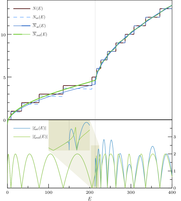
Figure 1: Spectrum for an interval with a potential step in the range $0\leq E\leq 400$. The lengths were chosen as $L_{1}=1$ and $L_{2}=\sqrt{3}$ and the potential step size as $V=213$. The threshold energy $E=V$ is indicated by a dashed vertical line.
Upper panel: Exact counting function $N(E$ (brown staircase) and expression $N_{\mathrm{at}}(E)$ (dashed blue line) and mean counting functions (full blue and green lines).
Lower panel: Secular functions.

Finally let us discuss the behavior far below threshold by considering $E\ll V$ in the asymptotic limit $V\to\infty$. In this limit any periodic orbit that visits the interval $x\in[L_{1},L]$ is suppressed exponentially leaving only contributions from the primitive orbit $\tilde{p}=\overline{1}$ and its repetitions

$${\overline{N}}_{\mathrm{red}}(E)\sim \frac{L_{1}\sqrt{E}}{\pi}-\frac{1}{2}+\frac{1}{2\pi}\mathrm{Im}\log\left(\frac{\sqrt{V-E}+i\sqrt{E}}{\sqrt{V-E}-i\sqrt{E}}\right)$$ (24)

$$N_{\mathrm{red},\mathrm{osc}}(E)\sim -\frac{1}{\pi}\mathrm{Im}\ \log\left(1-U_{11}\right)\ .$$ (25)

Note that $U_{11}=-\frac{\sqrt{E}-i\sqrt{V-E}}{\sqrt{E}+i\sqrt{V-E}}e^{2iL_{1}\sqrt{E}}$ is unimodular for $E<V$ and we have only neglected exponentially small terms while keeping any corrections of order $\mathcal{O}\left((E/V)^{n}\right)$ for arbitrary large $n$. Moreover, we have used $\frac{1}{2\pi}\mathrm{Im}\log\left(-[U^{-1}]_{22}\right)=\frac{1}{2\pi}\mathrm{Im}\log\left(\frac{\sqrt{V-E}+i\sqrt{E}}{\sqrt{V-E}-i\sqrt{E}}\right)$ in the mean counting function. This contribution shifts the counting function by values

$$0\leq\frac{1}{2\pi}\mathrm{Im}\log\left(\frac{\sqrt{V-E}+i\sqrt{E}}{\sqrt{V-E}-i\sqrt{E}}\right)\leq\frac{1}{2},$$ (26)

and increases from the lower bound to the upper bound as $E$ increases from zero to $V$.

Let us illustrate this with a numerical example. In Figure 1 we plot counting functions in the upper and the absolute value of the secular function in the lower panel for a specific (arbitrary) choice of parameters (see figure caption). The exact counting function $N(E)$ (fat brown staircase line) and the expression $N_{\mathrm{at}}(E)$ (dashed blue line) given by (13a) only coincide above threshold $E>V$. Below threshold $N_{\mathrm{at}}(E)$ shows steps at the energy eigenvalues but the plateau between steps is not constant. It has an additional step of half size at the threshold $E=V$ This may all be expected from the fact that the secular function has a spurious zero at threshold and is defined in terms of a unitary matrix only above threshold.
The upper panel also contains plots of the mean counting functions $\overline{N}_{\mathrm{red}}(E)$ (green line) and $\overline{N}_{\mathrm{at}}(E)$ (blue line) as given by the trace formulas (21b) and (13b). Above threshold both trace formulas coincide for the full counting function but give different divisions into a ‘mean’ and ‘oscillating’ part. Comparing the two ‘mean’ parts above threshold it is apparent that $\overline{N}_{\mathrm{red}}(E)$ oscillates around $\overline{N}_{\mathrm{at}}(E)$. Indeed the difference of the two corresponds to periodic orbits that remain inside the edge $x>L_{1}$ which are oscillatory functions of the energy for $E>V$ with an amplitude that decays with $E\to\infty$ (when the potential step becomes more and more transparent). So one may view $\overline{N}_{\mathrm{at}}(E)$ as the more natural candidate for the mean part above threshold. We have therefore plotted $\overline{N}_{\mathrm{at}}(E)$ with a fatter line in this region. Below threshold $E<V$ both $\overline{N}_{\mathrm{at}}(E)$ and $\overline{N}_{\mathrm{red}}(E)$ are smooth increasing functions. However only $\overline{N}_{\mathrm{red}}(E)$ is related to an exact trace formula for the counting function. One can see that the mismatch between the exact counting function $N(E)$ and the trace formula $N_{\mathrm{at}}(E)$ is due to the fact that the corresponding ‘mean’ part $\overline{N}_{\mathrm{at}}(E)$ is too low by the same amount. The more natural choice for the mean part below threshold is clearly $\overline{N}_{\mathrm{red}}(E)$ which is therefore drawn with a fat line for $E<V$. But this means that the natural choice for the mean part of the counting function switches from the expression (21b) for $\overline{N}_{\mathrm{red}}(E)$ to (13b) for $\overline{N}_{\mathrm{at}}(E)$ at $E=V$. The two expressions do not fit together continuously at threshold however.

The lower panel in Figure 1 shows the absolute value of the secular functions $\xi(E)$ and $\xi_{\mathrm{red}}(E)$ (equations (12) and (20)). Away from the threshold their zeros coincide and clearly correspond to the increases of the counting function. The ratio of the two satisfies

$$\frac{\xi(E)}{\xi_{\mathrm{red}}(E)}=1-U_{22}=1-\frac{k_{1}-k_{2}}{k_{1}+k_{2}}e^{i2L_{2}k_{2}}\ .$$ (27)

At threshold $U_{22}=1$ and this is the reason for the different behavior of the two secular functions at this energy (see magnified region of the plot). Below threshold $|U_{22}|=e^{-2\sqrt{V-E}L_{2}}$ and (27) approaches unity exponentially when $E$ is decreased and this can clearly be seen in the plots which lie on top of each other until one gets close to threshold from below. Above threshold $|U_{22}|=\frac{\sqrt{E}-\sqrt{E-V}}{\sqrt{E}+\sqrt{E-V}}\sim\frac{V}{E}$ (when $E\gg V$). So the ratio also tends to unity when moving away from threshold but only with a slow $V/E$ decay and this is consistent with the plot.

III Schrödinger operators on quantum graphs for the piecewise constant potentials and multi-mode models

The main aim of the remainder of this manuscript is to derive a generalization of the trace formulas which were presented in the previous section to quantum graphs with piecewise constant potentials or multiple modes. The details will be given in Sections IV and V. Before doing so we shall summarize in this section the standard description of PCP quantum graphs as self-adjoint metric Schrödinger operators on metric graphs with appropriate matching conditions following schrader ; grisha_book ; kuchment . In most applications of quantum graphs one assumes a zero potential on the edges. The addition of piecewise constant potentials is straight forward and therefore readers that are familiar with quantum graphs may skip most of this – or just pick up the notation. We shall then proceed to describe the relation between the differential operators in the PCP an MM models.

A quantum graph consists of a metric graph $\mathcal{G}$ and a self-adjoint Schrödinger operator $\hat{H}$ in the Hilbert space $L^{2}(\mathcal{G})$ of square-integrable functions on $\mathcal{G}$ grisha_book ; schrader ; kuchment . Without loss of generality we assume that the graph is connected. We allow the graph to have parallel edges and loops but we will assume here that the metric graph is compact. In that case the graph has a finite number $N_{V}$ of vertices and a finite number $N_{E}$ of edges. Each edge $e$ has a (finite) length $L_{e}>0$ and a coordinate $x_{e}\in[0,L_{e}]$ that describes individual points on the edge such that $x_{e}=0$ and $x_{e}=L_{e}$ are the vertices to which the edge is attached. The explicit choice of direction is arbitrary: $L_{e}-x_{e}$ is as good a coordinate on $e$ as $x_{e}$.
The Schrödinger operator $\hat{H}$ is defined on a dense subspace of $L^{2}(\mathcal{G})\equiv\oplus_{e\in\mathcal{G}}L^{2}\left([0,L_{e}]\right)$ (to be discussed below). Any wavefunction $\boldsymbol{\Phi}$, (that is, any element of this subspace) is a collection of $N_{E}$ complex scalar functions $\boldsymbol{\Phi}_{e}\equiv\phi_{e}(x_{e})\in L^{2}([0,L_{e}])$ and the Schrödinger operator acts as

$$\left(\hat{H}\boldsymbol{\Phi}\right)_{e}=-\frac{d^{2}\phi_{e}}{dx_{e}^{2}}(x_{e})+V_{e}\phi_{e}(x_{e})\ .$$ (28)

Here $V_{e}\in\mathbb{R}$ is a potential that is constant on each edge. Piecewise constant potentials can be accommodated by adding vertices at the positions where the value of the potential changes. In order for the Schrödinger operator to be well-defined one needs to make sense of the second derivative in a weak way grisha_book . For this one needs $\phi_{e}(x_{e})$ to be a continuous square-integrable function which is piecewise differentiable. For the stronger requirement that $\hat{H}$ defines a self-adjoint operator one needs additional matching conditions at the vertices. There is no unique choice of matching conditions and the most general set of matching conditions can be described in several equivalent ways. We follow the description of Schrader and Kostrykin schrader . Let us consider one vertex $v$ and denote its degree by $d_{v}$. Let $\mathbf{S}(v)$ be the star of $v$. By definition this is set of edges connected to $v$ (where any loops are considered as two independent edges by adding an auxiliary vertex). Clearly $\left|\mathbf{S}(v)\right|=d_{v}$. For any edge $e\in\mathbf{S}(v)$ we may assume without loss of generality that $x_{e}=0$ corresponds to the vertex $v$ on which we focus. The matching conditions are a set of $d_{v}$ simultaneous linear relations between the wavefunction and their derivatives at $x_{e}=0$ for all $e\in\mathbf{S}(v)$

$$\sum_{e^{\prime}\in\mathbf{S}(v)}\left(A_{ee^{\prime}}\phi_{e^{\prime}}(0)+B_{ee^{\prime}}\frac{d\phi_{e^{\prime}}}{dx_{e^{\prime}}}(0)\right)=0\ .$$ (29)

There are $d_{v}$ equations, one for each edge $e\in\mathbf{S}(v)$. The coefficients $A_{ee^{\prime}}$ and $B_{ee^{\prime}}$ form two complex $d_{v}\times d_{v}$ matrices $A$ and $B$ for which one requires that $AB^{\dagger}=BA^{\dagger}$ is a hermitian matrix and that the $d_{v}\times 2d_{v}$ matrix $(A,B)$ has maximal rank $d_{v}$. Note that $A\mapsto CA$ and $B\mapsto CB$ for an invertible matrix $C$ gives equivalent matching conditions.

If one chooses matrices $A$ and $B$ with the above conditions for each vertex $v$ in $\mathcal{G}$ then the self-adjoint Schrödinger operator $\hat{H}$ is defined on the dense subspace of $L^{2}(\mathcal{G})$ of piecewise differentiable wavefunctions that satisfy the corresponding matching conditions at all vertices.

In sections IV and V we will consider the eigenproblem

$$\hat{H}\boldsymbol{\Phi}=E\boldsymbol{\Phi}\ ,$$ (30)

that is the stationary Schrödinger equation on the graph.

In a MM quantum graph the scalar wave function on a given edge is replaced by a multi-component wavefunction. The various components describe the transversal modes that may be excited above a threshold energy. In the present setting we always assume a finite number of modes. This is essential to ensure a discrete energy spectrum. Quantum graphs with infinitely many modes and spectra that contain continuous bands have been considered smilansky_model .

One arrives at a Schrödinger operator on a MM graph by generalizing on one side (28) to the MM setting by adding a diagonal matrix that includes excitation energies for each transversal mode. On the other side one generalizes the matching conditions (29) by replacing the matrices $A_{e,e^{\prime}}$ and $B_{e,e^{\prime}}$ by matrices with elements which carry a double index : $A_{(e,m),(e^{\prime},m^{\prime})}$ and $B_{(e,m),(e^{\prime},m^{\prime})}$ where $e,e^{\prime}\in\mathcal{S}(v)$ identify the interacting edges and the $m,m^{\prime}$ identify the interacting modes. We give the details of this description in Appendix A.

A formally equivalent PCP quantum graph can be constructed by replacing each edge of a MM graph by parallel single-mode edges of the same length. The details of this construction can also be found in Appendix A. The main difference between the PCP and MM models is in different physical choices of matching conditions at the vertices.

IV The scattering approach

The scattering approach to a quantum graph with $N_{V}$ vertices and $N_{E}$ edges has been a very useful tool for spectral analysis in the single-mode case without potentials KS_traceformula ; review . There, it leads to an explicit quantization condition in terms of the zeros of a spectral determinant $\xi(E)=\det\left(\mathbb{I}-U(E)\right)=0$ where $U(E)$ is a unitary matrix of dimension $2N_{E}\times 2N_{E}$ known as the quantum map. The quantum map is built up as a product of matrices that describe scattering at each vertex followed by transport along the edges. In this section we will generalize the scattering approach to MM and PCP quantum graphs. The explicit formulation will follow the PCP model which includes the MM model via the formal equivalence as was discussed in the previous section and Appendix A.

In the presence of edge potentials the scattering matrix need not be unitary as some edges may support evanescent modes. Conservation of probability currents in this case follows from a well-known symmetry of scattering matrices in the presence of evanescent modes weidenmueller that we will derive explicitly from the general matching conditions.

IV.1 The vertex scattering matrices and its properties

Let us consider one vertex $v$ of degree $d$. Without loss of generality we choose the coordinates $x_{e}$ on the adjacent edges such that $x_{e}=0$ is the location of the vertex $v$ and we enumerate the edges of the graph such that $e=1,\dots,d$ correspond to the adjacent edges. Collecting the wavefunctions on the adjacent edges in a column vector $\boldsymbol{\phi}(\boldsymbol{x})=(\phi_{1}(x_{1}),\dots,\phi_{d}(x_{d}))^{T}$ where $\boldsymbol{x}=(x_{1},x_{2},\dots,x_{d})$ is the collection of coordinates we may rewrite the matching conditions (29) in matrix form as

$$A\boldsymbol{\phi}(0)+B\boldsymbol{\phi}^{\prime}(0)=0\ .$$ (31)

At a given energy $E$ the solution of the differential equation (28) can be expressed in terms of plane wave propagating in opposite directions. Combining these we may write a wavefunction that solves the differential equation on all adjacent edges as

$$\boldsymbol{\phi}(\boldsymbol{x})=\frac{1}{\sqrt{K}}e^{iKX}\boldsymbol{b}_{\mathrm{out}}+\frac{1}{\sqrt{K}}e^{-iKX}\boldsymbol{b}_{\mathrm{in}}$$ (32)

where $X$ is a diagonal matrix with diagonal $\boldsymbol{x}$ and $K$ is a diagonal matrix $K_{ee^{\prime}}=\delta_{e^{\prime}}K_{e}$ with the wavenumbers

$$K_{e}=\sqrt{E-V_{e}}$$ (33)

for each adjacent edge. Note that $K_{e}\geq 0$ for $E\geq V_{e}$. For $E<V_{e}$ the wavenumber is imaginary and we choose the convention $K_{e}=i|K_{e}|$ in this case (positive imaginary part). This choice is consistent with implicit limits $\epsilon\to 0^{+}$ in the energy $E\mapsto E+i\epsilon$ that will appear in the next section. In this case the two solutions are increasing or decreasing exponential functions. The factors $\frac{1}{\sqrt{K}}$ in (32) normalize the plane wave solutions $\frac{1}{\sqrt{K_{e}}}e^{iK_{e}x_{e}}$ to unit probability flux (for $E>V_{e}$). As $K_{e}=0$ at $E=V_{e}$ we have to assume that the energy is not equal to any of the potentials on adjacent edges. Finally $\boldsymbol{b}_{\mathrm{in/out}}$ denotes $d$-dimensional column vectors that contain the amplitudes of the incoming and outgoing waves. Note that the direction of a plane wave implied here is the direction of the corresponding flow for $E>V_{e}$ and the direction of exponential decay for $E<V_{e}$. The matching conditions (31) allow us to express the outgoing amplitudes in terms of the incoming amplitudes as

$$\boldsymbol{b}_{\mathrm{out}}=\sigma(K)\boldsymbol{b}_{\mathrm{in}}$$ (34)

with the $d\times d$ vertex scattering matrix

$$\sigma(K)=-K^{1/2}\frac{\mathbb{I}}{A+iBK}\left(A-iBK\right)K^{-1/2}=-\mathbb{I}+2iK^{1/2}\frac{\mathbb{I}}{A+iBK}BK^{1/2}\ .$$ (35)

If all potentials $V_{e}$ vanish, one may replace the matrix $K$ by the real positive wavenumber $k=\sqrt{E}$ and the expression reduces to the well-known formula for the energy-dependent unitary vertex scattering matrix schrader for standard quantum graphs (with vanishing edge potentials). If the potentials do not vanish then the vertex scattering matrix is in general not unitary. One may however express it in terms of the unitary matrix

$$\mathcal{S}\equiv\sigma(\mathbb{I})=-\frac{\mathbb{I}}{A+iB}\left(A-iB\right)=-\mathbb{I}+2i\frac{\mathbb{I}}{A+iB}B\ .$$ (36)

Unitarity of $\mathcal{S}$ follows straight forwardly from the conditions that $(A,B)$ has full rank and that $A^{\dagger}B=B^{\dagger}A$ is Hermitian. Indeed this is just the scattering matrix without potentials at energy $E=1$ (or equivalently if all potentials have the same value and we take the energy to be one unit above the potential). The relation between $\sigma(K)$ and $\mathcal{S}$ may be written as

$$\sigma(K)=\mathcal{R}+\mathcal{T}\frac{\mathbb{I}}{\mathbb{I}+\mathcal{S}\mathcal{R}}\mathcal{S}\mathcal{T}$$ (37)

where

$$\mathcal{R}=\frac{K-\mathbb{I}}{K+\mathbb{I}}\qquad\text{and}\qquad\mathcal{T}=\frac{2K^{1/2}}{K+\mathbb{I}}\ .$$ (38)

The relation (37) is easily checked algebraically and has a straight forward physical interpretation in terms of potential barriers on each edge which may be taken from the following sketch:

(39)

For this one imagines a small region of size $\delta>0$ around the vertex in which the potential has a constant value $V_{0}\equiv E-1$ and potential barriers at the distance $\delta$. Behind the barrier the potential is equal to the given edge potential. The positions of barriers form a set of $d$ additional vertices. One then obtains $\sigma(K)$ as the effective scattering matrix of the combined barriers and central vertex with scattering matrix $\mathcal{S}$ in the limit $\delta\to 0$ by observing that $\mathcal{R}$ is the diagonal matrix of reflection coefficients for direct reflection at the barrier without entering the vertex, $\mathcal{T}$ is the diagonal matrix of transmission coefficients across the barrier in either direction, and $-\mathcal{R}$ gives the reflection at the barrier from the vertex back into the vertex. Clearly, (37) just describes the sum of a direct reflection from the barrier plus a term that describes the transmission through the barrier followed by scattering at the vertex and multiple back-reflection into the vertex before the final transmission back into the edge. This is consistent with the scattering matrix (7) at a potential step (considered as a vertex of degree two) in two ways. On one side the reflection and transmission coefficients on the diagonal of $\mathcal{R}$ and $\mathcal{T}$ are obtained from (7) at unit energy. On the other side one obtains back (7) at arbitrary energy by using (37) with $\mathcal{S}$ as a pure transmission matrix describing continuity of the wavefunction and its derivative.

For $E>V_{e}$ on all adjacent edges $K$ is a real diagonal matrix and one finds that $\sigma(K)$ is unitary. This can be shown starting from (37) and using the unitary of $\mathcal{S}$. In general there will be some edges where $E<V_{e}$ and the solutions are evanescent (exponential). To discuss the structure of the scattering matrix in this case let us assume that the edges are enumerated such that $V_{1}\leq V_{2}\leq\dots V_{d}$ and consider an energy $E\in(V_{e_{0}},V_{e_{0}+1}$ for some edge $e_{0}\in\{1,\dots,d-1\}$ (the cases $E<V_{1}$ and $E>V_{d}$ follow straight forwardly from the following discussion). Then one has oscillatory solutions on the edges on the edges $e=1,2,\dots,e_{0}$ and evanescent solutions on the remaining edges $e=e_{0}+1,\dots,d$. Let us write all matrices as block matrices. For the vertex scattering matrix one then has

$$\sigma(K)=\begin{pmatrix}\sigma(K)_{\mathrm{osc},\mathrm{osc}}&\sigma(K)_{\mathrm{osc},\mathrm{ev}}\\ \sigma(K)_{\mathrm{ev},\mathrm{osc}}&\sigma(K)_{\mathrm{ev},\mathrm{ev}}\end{pmatrix}$$ (40)

where the index $\mathrm{osc}$ stands for oscillatory and $\mathrm{ev}$ for evanescent. The diagonal blocks $\sigma(K)_{\mathrm{osc},\mathrm{osc}}$ and $\sigma(K)_{\mathrm{ev},\mathrm{ev}}$ are square matrices of dimension $e_{0}\times e_{0}$ and $(d-e_{0})\times(d-e_{0})$. The other off-diagonal blocks $\sigma(K)_{\mathrm{osc},\mathrm{ev}}$ and $\sigma(K)_{\mathrm{ev},\mathrm{osc}}$ are in general rectangular of dimension $e_{0}\times(d-e_{0})$ and $(d-e_{0})\times e_{0}$. The diagonal matrix $K$ has real positive elements on the diagonal in the $\mathrm{osc}-\mathrm{osc}$ block and positive imaginary entries in the $\mathrm{ev}-\mathrm{ev}$ block. Unitarity of $\mathcal{S}$ and the properties of the matrix $K$ lead to the following symmetry properties for the blocks of the vertex scattering matrix

$$\left(\sigma(K)_{\mathrm{osc},\mathrm{osc}}\right)^{\dagger}\sigma(K)_{\mathrm{osc},\mathrm{osc}}= \mathbb{I},$$ (41a)

$$i\left(\sigma(K)_{\mathrm{osc},\mathrm{ev}}\right)^{\dagger}\sigma(K)_{\mathrm{osc},\mathrm{osc}}= \sigma(K)_{\mathrm{ev},\mathrm{osc}},$$ (41b)

$$i\sigma(K)_{\mathrm{osc},\mathrm{osc}}\left(\sigma(K)_{\mathrm{ev},\mathrm{osc}}\right)^{\dagger}= \sigma(K)_{\mathrm{osc},\mathrm{ev}},$$ (41c)

$$i\left(\sigma(K)_{\mathrm{osc},\mathrm{ev}}\right)^{\dagger}\sigma(K)_{\mathrm{osc},\mathrm{ev}}= \sigma(K)_{\mathrm{ev},\mathrm{ev}}-\left(\sigma(K)_{\mathrm{ev},\mathrm{ev}}^{\dagger}\right)\ .$$ (41d)

Here the third equation follows directly from the first two equations. The rest can be found by direct calculation. These symmetries are well-known in the general context of scattering when evanescent modes are present weidenmueller ; schanz ; rouvinez . Each of the four equations can be related to flux conversation brewer . Observing that the outgoing flux on an adjacent edge is given by

$$I_{e}=\begin{cases}|b_{\mathrm{out},e}|^{2}-|b_{\mathrm{in},e}|^{2}&\text{for $e\leq e_{0}$;}\\ 2\ \mathrm{Im}\ b_{\mathrm{in},e}^{*}b_{\mathrm{out},e}&\text{for $e>e_{0}$.}\end{cases}$$ (42)

then the conditions (41) ensure

$$\sum_{e=1}^{d}I_{e}=0$$ (43)

for arbitrary choice of the incoming amplitudes $\boldsymbol{a}_{\mathrm{in}}$.

IV.2 The quantum map and the quantization condition

Let us now look at the collection of all vertex scattering matrices $\sigma^{(v)}(K)$ for $v=1,\dots,N_{V}$ at a given energy $E$. We will assume throughout that $E$ is not equal to any of the constant potentials on one of the edges. Each of these matrices acts on the incoming amplitudes $\boldsymbol{b}^{(v),\mathrm{in}}$ of plane waves at the given vertex and results in the outgoing amplitudes at the same vertex $\boldsymbol{b}^{(v),\mathrm{out}}=\sigma^{(v)}(K)\boldsymbol{b}^{(v),\mathrm{in}}$. We may collect all incoming an outgoing amplitudes at all vertices in two $2N_{E}$ dimensional vectors $\boldsymbol{b}^{\mathrm{in}}$ and $\boldsymbol{b}^{\mathrm{out}}$ such that each component corresponds to one directed edge. One may the introduce the $2N_{E}\times 2N_{E}$ graph scattering matrix $S(E)$ such that

$$\boldsymbol{b}^{\mathrm{out}}=S(E)\boldsymbol{b}^{\mathrm{in}}\ .$$ (44)

One can then order the incoming amplitudes in such a way that the graph scattering matrix is a product of two matrices

$$S(E)=P\Sigma(K)$$ (45)

with the block-diagonal matrix

$$\Sigma(K)=\begin{pmatrix}\sigma^{(1)}(K)&0&\dots&0\\ 0&\sigma^{(2)}(K)&\dots&0\\ \dots&\dots&\dots&\dots\\ 0&0&\dots&\sigma^{(N_{V})}(K)\end{pmatrix}$$ (46)

that contains the vertex scattering matrices on the diagonal and a permutation matrix $P$. With the convention that we order both amplitude vectors in the same order with respect to directed edges (where ‘in’ and ‘out’ give the sense of direction) the permutation matrix $P$ just interchanges the two directions on the same edge. Note that equation (37) remains valid when replacing $\sigma(K)\mapsto\Sigma(K)$ if the matrices $\mathcal{S}$, $K$, $\mathcal{R}$ and $\mathcal{T}$ are extended to $2N_{E}\times 2N_{E}$ matrices. Note that the permutation matrix $P$ commutes with $K$, $\mathcal{R}$ and $\mathcal{T}$, as these are diagonal matrices with the same entries for either direction on a given edge. Reordering the matrix $\Sigma(K)$ with respect to oscillating and evanescent modes on the edges for a given energy $E$ the symmetries (41) also hold for $\sigma(K)\mapsto\Sigma(K)$.

Next, the local plane wave solutions directly connect the outgoing amplitude from the start vertex to the incoming amplitude at the end vertex of a directed edge. This gives the relation

$$\boldsymbol{b}^{\mathrm{in}}=T(E)\boldsymbol{b}^{\mathrm{out}}\ .$$ (47)

with the diagonal matrix

$$T(E)=e^{iKL}$$ (48)

in terms of the two diagonal matrices $K$ (wavenumbers) and $L$ (edge lengths). The two equations (44) and (48) result in the condition

$$\boldsymbol{b}^{\mathrm{in}}=U(E)\boldsymbol{b}^{\mathrm{in}}$$ (49)

with the so-called quantum map

$$U(E)=T(E)S(E)=T(E)P\Sigma(K)=PT(E)\Sigma(K)\ .$$ (50)

In the following the explicit dependence on the energy $E$ or the wavenumber matrix $K$ will often be dropped for better readability. The quantization condition may also be written in terms of the secular equation

$$\xi(E)\equiv\mathrm{det}\left(\mathbb{I}-U(E)\right)=0$$ (51)

with the secular function $\xi(E)$.
Let us now fix an energy $E>\mathrm{min}_{e}(V_{e})$ and order the directed edges according to increasing potentials. The corresponding permutation matrix is unitary and thus does not change the structure of the quantum map (50). We introduce the oscillatory and evanescent blocks in the same way as in the discussion of the vertex scattering matrix above: The directed edges $e$ where $E>V_{e}$ have oscillatory solutions (superpositions of plane waves) and form the oscillatory subspace where the remaining edges with $E<V_{e}$ form the evanescent subspace (which may be empty if $E>\mathrm{max}_{e}(V_{e})$). Writing all matrices in block form the quantum map becomes

$$U\equiv\begin{pmatrix}U_{\mathrm{osc},\mathrm{osc}}&U_{\mathrm{osc},\mathrm{ev}}\\ U_{\mathrm{ev},\mathrm{osc}}&U_{\mathrm{ev},\mathrm{ev}}\end{pmatrix}\ .$$ (52)

Then $U$ inherits from (41) the symmetries

$$U_{\mathrm{osc},\mathrm{osc}}^{\dagger}U_{\mathrm{osc},\mathrm{osc}}= \mathbb{I}$$ (53a)

$$i\left(U_{\mathrm{osc},\mathrm{ev}}\right)^{\dagger}U_{\mathrm{osc},\mathrm{osc}}= P_{\mathrm{ev},\mathrm{ev}}T_{\mathrm{ev},\mathrm{ev}}^{-1}U_{\mathrm{ev},\mathrm{osc}}$$ (53b)

$$iU_{\mathrm{osc},\mathrm{osc}}\left(U_{\mathrm{ev},\mathrm{osc}}\right)^{\dagger}= U_{\mathrm{osc},\mathrm{ev}}P_{\mathrm{ev},\mathrm{ev}}T_{\mathrm{ev},\mathrm{ev}}$$ (53c)

$$i\left(U_{\mathrm{osc},\mathrm{ev}}\right)^{\dagger}U_{\mathrm{osc},\mathrm{ev}}= P_{\mathrm{ev},\mathrm{ev}}T_{\mathrm{ev},\mathrm{ev}}^{-1}U_{\mathrm{ev},\mathrm{ev}}-U_{\mathrm{ev},\mathrm{ev}}^{\dagger}P_{\mathrm{ev},\mathrm{ev}}T_{\mathrm{ev},\mathrm{ev}}^{-1}$$ (53d)

where we have used that the permutation matrix $P=P^{-1}=P^{\dagger}$ is block-diagonal (as it transposes directions on the same edge) and the $\mathrm{ev}-\mathrm{ev}$ block of the transport matrix is real diagonal.
If $E>\mathrm{max}_{e}(V_{e})$ the quantum map is unitary. In that case it is straight forward to derive a trace formula that counts the number of states below a given energy $E$ using standard methods. If $E<\mathrm{max}_{e}(V_{e})$ then the quantum map is not unitary and deriving a trace formula is not as straight forward and it is the topic of the following section.

V The trace formula and its application

In the remainder of the manuscript we will focus on developing a trace formula that counts the number of states below a given energy $E$. For $E<\mathrm{max}_{e}(V_{e})$ we will first develop a reduced unitary description following ideas from brewer where analogous considerations have been used to deal with evanescent modes in graph-like structures of mechanical beams. Once a unitary description is in place we can use standard methods. We will assume throughout this chapter that the potentials are ordered $V_{e}<V_{e+1}$ and $E>V_{1}=\mathrm{min}_{e}(V_{e})$. Our trace formula will count the number of eigenenergies above this threshold. This is analogous to the situation in quantum graphs where the trace formula for the spectral counting function for a quantum graph with general self-adjoint matching conditions bolte only counts the number of states with positive energies while the number of negative energy states is finite and needs to be determined separately to obtain the full spectral counting function.

V.1 The reduced quantum map

For the given energy $E$ we use the corresponding division of the amplitudes $\mathbf{b}^{\mathrm{in}}$ in oscillatory and evanescent subspaces. Equivalently, we can refer to the evanescent and oscillatory subgraph. Writing the quantization condition in block-forms

$$U_{\mathrm{osc},\mathrm{osc}}\mathbf{b}^{\mathrm{in}}_{\mathrm{osc}}+U_{\mathrm{osc},\mathrm{ev}}\mathbf{b}^{\mathrm{in}}_{\mathrm{ev}}= \mathbf{b}^{\mathrm{in}}_{\mathrm{osc}}$$ (54a)

$$U_{\mathrm{ev},\mathrm{osc}}\mathbf{b}^{\mathrm{in}}_{\mathrm{osc}}+U_{\mathrm{ev},\mathrm{ev}}\mathbf{b}^{\mathrm{in}}_{\mathrm{ev}}= \mathbf{b}^{\mathrm{in}}_{\mathrm{ev}}\ .$$ (54b)

Assuming that $U_{\mathrm{ev},\mathrm{ev}}$ has no unit eigenvalue (see discussion below) we may rewrite the second equation as $\mathbf{b}^{\mathrm{in}}_{\mathrm{ev}}=\left(\mathbb{I}-U_{\mathrm{ev},\mathrm{ev}}\right)^{-1}U_{\mathrm{ev},\mathrm{osc}}\mathbf{b}^{\mathrm{in}}_{\mathrm{osc}}$ which allows us to reduce the quantization condition to a condition on the oscillatory part only

$$U_{\mathrm{red}}\mathbf{b}^{\mathrm{in}}_{\mathrm{osc}}=\mathbf{b}^{\mathrm{in}}_{\mathrm{osc}}$$ (55)

with the reduced quantum map

$$U_{\mathrm{red}}=U_{\mathrm{osc},\mathrm{osc}}+U_{\mathrm{osc},\mathrm{ev}}\frac{\mathbb{I}}{\mathbb{I}-U_{\mathrm{ev},\mathrm{ev}}}U_{\mathrm{ev},\mathrm{osc}}\ .$$ (56)

Physically, flux conservation now requires that the reduced map be unitary

$$U_{\mathrm{red}}^{\dagger}U_{\mathrm{red}}=\mathbb{I}.$$ (57)

Indeed this follows directly from the symmetries (53) between the blocks of the full quantum map.

The determinants of the full quantum map and the reduced quantum map obey the identities

$$\frac{\mathrm{det}\ U_{\mathrm{red}}}{\mathrm{det}\ U}=\frac{\det\left(\mathbb{I}-\left(U^{-1}\right)_{\mathrm{ev},\mathrm{ev}}\right)}{\det\left(\mathbb{I}-U_{\mathrm{ev},\mathrm{ev}}\right)}$$ (58)

and

$$\mathrm{det}\left(\mathbb{I}-U\right)=\mathrm{det}\left(\mathbb{I}-U_{\mathrm{ev},\mathrm{ev}}\right)\ \mathrm{det}\left(\mathbb{I}-U_{\mathrm{red}}\right)$$ (59)

where $\left(U^{-1}\right)_{\mathrm{ev},\mathrm{ev}}=\frac{\mathbb{I}}{U_{\mathrm{ev},\mathrm{ev}}-U_{\mathrm{ev},\mathrm{osc}}U_{\mathrm{osc},\mathrm{osc}}^{-1}U_{\mathrm{osc},\mathrm{ev}}}$ is the $\mathrm{ev}-\mathrm{ev}$ block of the inverse map $U^{-1}$. These identities may be derived straight forwardly purely from the definition of the reduced matrix from the full matrix (under the assumption that all involved matrices exist). We will use both identities later to write the trace formula in a precise yet intuitively appealing way.

Before turning to the trace formula let us comment on the implicit assumption that $\frac{\mathbb{I}}{\mathbb{I}-U_{\mathrm{ev},\mathrm{ev}}}$ exists in order to define the reduced map. Let us consider in more detail the situation when this assumption fails and assume that for some energy $E$ this inverse does not exist. Identity (59) suggests that the energy $E$ is in the spectrum as one of the factors in the secular equation vanishes. However, the reduced matrix is not defined and one may question whether the second factor remains finite. So let us demonstrate more carefully that indeed the energy is in the spectrum. As $U_{\mathrm{ev},\mathrm{ev}}$ has (at least one) unit eigenvalue we may denote the corresponding eigenvector as $\boldsymbol{\hat{b}}_{\mathrm{ev}}$. We claim that this eigenvector can be extended to an eigenvector with unit eigenvalue of the full quantum map

$$\begin{pmatrix}U_{\mathrm{osc},\mathrm{osc}}&U_{\mathrm{osc},\mathrm{ev}}\\ U_{\mathrm{ev},\mathrm{osc}}&U_{\mathrm{ev},\mathrm{ev}}\end{pmatrix}\begin{pmatrix}0\\ \boldsymbol{\hat{b}}_{\mathrm{ev}}\end{pmatrix}=\begin{pmatrix}0\\ \boldsymbol{\hat{b}}_{\mathrm{ev}}\end{pmatrix}\ .$$ (60)

To prove this one needs to show $U_{\mathrm{osc},\mathrm{ev}}\boldsymbol{\hat{b}}_{\mathrm{ev}}=0$. We do this by considering the squared norm $\left\|U_{\mathrm{osc},\mathrm{ev}}\boldsymbol{\hat{b}}_{\mathrm{ev}}\right\|^{2}=\left(\boldsymbol{\hat{b}}_{\mathrm{ev}}\right)^{\dagger}U_{\mathrm{osc},\mathrm{ev}}^{\dagger}U_{\mathrm{osc},\mathrm{ev}}\boldsymbol{\hat{b}}_{\mathrm{ev}}=0$ where the last equality follows from the symmetry property (53d) and using that $\boldsymbol{\hat{b}}_{\mathrm{ev}}$ is a unit eigenvector of $U_{\mathrm{ev},\mathrm{ev}}$. The extended eigenvector corresponds to a wave function on the graph that is completely confined to the evanescent subgraph. While this is possible (e.g. when there are vertices inside the evanescent part with attracting $\delta$-type matching conditions) it requires fine-tuning – a small change of edge lengths or matching conditions will deform this eigenstate to a new one at a shifted energy such that it leaks out into the full graph. By using the spectral decomposition of $U_{\mathrm{ev},\mathrm{ev}}$ near the energy where it is not invertible one can then define the reduced map $U_{\mathrm{red}}$ continuously in a neighborhood. However the identity (59) shows that the reduced secular function

$$\xi_{\mathrm{red}}(E)=\det\left(\mathbb{I}-U_{\mathrm{red}}(E)\right)$$ (61)

is generally not zero at an energy $E$ where $U_{\mathrm{ev},\mathrm{ev}}$ has a unit eigenvalue though we have just shown that it is in the spectrum. A trace formula based on the quantization condition $\xi_{\mathrm{red}}(E)=0$ may thus miss some states. For the remainder we will assume that $U_{\mathrm{ev},\mathrm{ev}}$ has no unit eigenvalues for any (relevant) energy. This is indeed generic as a small change of parameters (lengths, potentials) will immediately lead to some leakage into the oscillatory part of the graph. In Section V.3 we construct this situation explicitly for some example graphs and investigate this numerically.

V.2 The trace formula

With a unitary reduced map $U_{\mathrm{red}}(E)$ and a quantization condition $\mathrm{det}\left(\mathbb{I}-U_{\mathrm{red}}(E)\right)=0$ Cauchy’s argument principle allows us to write the spectral counting function (or staircase function) as the trace formula

$$N(E)= \overline{N}(E)+N_{\mathrm{osc}}(E)$$ (62a)

$$\overline{N}(E)= \frac{1}{2\pi}\mathrm{Im}\ \log\mathrm{det}\left(U_{red}(E+i\epsilon)\right)+c$$

$$= \sum_{e=1}^{N_{E}}\theta(E-V_{e})\frac{L_{e}\sqrt{E-V_{e}}}{\pi}+\frac{1}{2\pi}\mathrm{Im}\ \log\mathrm{det}\left(S(E+i\epsilon)\right)+c$$

$$+\frac{1}{2\pi}\mathrm{Im}\ \log\mathrm{det}\left(\mathbb{I}-\left(U(E+i\epsilon)^{-1}\right)_{\mathrm{ev},\mathrm{ev}}\right)-\frac{1}{2\pi}\mathrm{Im}\ \log\mathrm{det}\left(\mathbb{I}-U_{\mathrm{ev},\mathrm{ev}}(E+i\epsilon)\right)$$ (62b)

$$N_{\mathrm{osc}}(E)= -\frac{1}{\pi}\mathrm{Im}\ \log\mathrm{det}\left(\mathbb{I}-U_{\mathrm{red}}(E+i\epsilon)\right)$$

$$= -\frac{1}{\pi}\mathrm{Im}\ \log\mathrm{det}\left(\mathbb{I}-U(E+i\epsilon)\right)+\frac{1}{\pi}\mathrm{Im}\ \log\mathrm{det}\left(\mathbb{I}-U_{\mathrm{ev},\mathrm{ev}}(E+i\epsilon)\right)$$

$$= \sum_{n=1}^{\infty}\frac{1}{n}\left(\mathrm{tr}\ U^{n}-\mathrm{tr}\ U_{\mathrm{ev},\mathrm{ev}}^{n}\right)={\sum_{p}}^{\prime}\sum_{r=1}^{\infty}\frac{1}{r}A_{p}^{r}e^{irW_{p}}$$ (62c)

which is valid for all energies $E>V_{1}=\mathrm{min}_{e}(V_{e})$. We have used the identities (58) and (59). Note that the individual expressions are not continuous at energies that equal to any potential $E=V_{e}$ as the dimension of the blocks and the reduced map change at these energies. The constant $c$ may be evaluated from requiring that $\lim_{E\to V_{1}^{+}}N(E)$ is equal to the number of eigenenergies smaller or equal to $V_{1}$. In the oscillatory part we have used $\log\mathrm{det}\ (\mathbb{I}-U)=\mathrm{tr}\ \log(\mathbb{I}-U)=-\sum_{n=1}^{\infty}\frac{1}{n}\mathrm{tr}\ U^{n}$ and wrote the traces as a sum over primitive periodic orbits $p$ on the graph. Let us denote a directed edge $\mathbf{e}$ as a pair $\mathbf{e}\equiv(e,d)$ where $e$ is an edge and $d=\pm$ is the direction (for some given choice of ‘positive’ and ‘negative’ direction). A periodic orbit of length $n$ is a cyclic sequence $\overline{\mathbf{e}_{1}\mathbf{e}_{2}\dots\mathbf{e}_{n}}\equiv\overline{\mathbf{e}_{2}\dots\mathbf{e}_{n}\mathbf{e}_{1}}$ of $n$ directed edges such the vertex at the end of $\mathbf{e}_{j}$ coincides with the vertex of the start of $\mathbf{e}_{j+1}$. Cyclic means $\mathbf{e}_{n+j}\equiv\mathbf{e}_{j}$ (the the start of $\mathbf{e}_{1}$ is the end of $\mathbf{e}_{n}$) and considering an equivalence class with respect to the starting edge. The periodic orbit is primitive if it is not the repetition of a shorter orbit. The sum on the right of (62c) expresses the oscillatory part of the counting function as a sum of contributions from primitive periodic orbits $p=\overline{\hat{e}_{1},\hat{e}_{2}\dots\hat{e}_{n_{p}}}$ of length $n_{p}$ and their repetitions $r$. To each primitive orbit one associates an amplitude $\prod_{j=1}^{n_{p}}U_{\hat{e}_{j+1}\hat{e}_{j}}\equiv A_{p}e^{iW_{p}}$ where $W_{p}=\sum_{j=1}^{n_{p}}K_{e_{j}}L_{e_{j}}$ and $A_{p}=\prod_{j=1}^{n_{p}}S_{\hat{e}_{j+1}\hat{e}_{j}}$ is the product of scattering matrix elements. The prime in the summation indicates that only primitive orbits that have at least one directed edge in the oscillatory subgraph contribute, that is the subgraph that consists of all edges with $V_{e}<E$. These are characterized by $\mathrm{Re}\ W_{p}\neq 0$. The contributions from these orbits are oscillatory because of the factor $e^{i\mathrm{Re}\ W_{p}}$ which is an oscillatory function of the energy. The imaginary part of $W_{p}$ corresponds to the evanescent edges that are visited and leads to an exponential suppression of these orbits due to a factor $e^{-\mathrm{Im}\ W_{p}}$. At a given energy one may distinguish three types of orbits $p$: either all edges of $p$ are in the evanescent part (for these orbits $\mathrm{Re}\ W_{p}=0$), or all edges of $p$ are in the oscillatory part (in this case $\mathrm{Im}\ W_{p}=0$) or $p$ visits both the evanescent and the oscillatory subgraphs. Only the latter two types have are contained in the oscillatory part of the counting function, and far below the next critical energy the orbits that are purely oscillatory orbits are dominant. We will show below that one part of the mean counting function (62b) contains contributions from purely evanescent periodic orbits.

One may wonder why the constant $c$ has the same value when the individual parts of the expression are not continuous at $E=V_{e}$. Should one not choose different constants in each interval such that the counting function remains continuous at these energies (or jumps by an integer if they happen to be in the spectrum). The reason for this lies in the fact that there is an element of choice in the formula that we have given. E.g. the reduced map as we have defined it has dimension two for energies $V_{1}<E<V_{2}$ and then changes to dimension four in the interval $V_{2}<V_{3}$ and so forth. Alternatively one may stick to a reduced map of dimension two for all energies $E>V_{1}$ without the restriction $E<V_{2}$. When crossing $E=V_{2}$ the two-dimensional reduced map remains unitary and the trace formula remains valid. Just the designation of the blocks as oscillatory and evanescent becomes blurred as the $\mathrm{ev}-\mathrm{ev}$ block now acts on a subgraph that has one oscillatory edge. The unitarity of this matrix across such a crossing can be shown explicitly and follows directly from the fact that one may reduce the matrix in steps and reducing an already unitary further will always lead to a smaller unitary matrix. Analogously the formula with a reduced matrix of given size $2e\times 2e$ is valid for all energies $E>V_{e}$. Eventually for $E>V_{N_{E}}$ one may use any of the $N_{E}-1$ reduced matrices, or the full matrix $U$. This does not imply that the individual terms $\overline{N}(E)$ and $N_{\mathrm{osc}}(E)$ are the same for all these choices – only their sum is not affected by this choice. This can be seen directly if we fix the dimension of the reduced matrix but consider the expression at energy $E>V_{N_{E}}$. At this energy the full matrix has become unitary $U^{-1}=U^{\dagger}$ such that $(U^{-1})_{\mathrm{ev},\mathrm{ev}}=(U^{\dagger})_{\mathrm{ev},\mathrm{ev}}=U_{\mathrm{ev},\mathrm{ev}}^{\dagger}$. In that case the third term in the expression for $\overline{N}(E)$ obeys $\mathrm{det}\left(\mathbb{I}-\left(U^{-1}\right)_{\mathrm{ev},\mathrm{ev}}\right)=\mathrm{det}\left(\mathbb{I}-U^{\dagger}_{\mathrm{ev},\mathrm{ev}}\right)=\mathrm{det}\left(\mathbb{I}-U_{\mathrm{ev},\mathrm{ev}}\right)^{*}$ which implies that the third and forth term can be combined to $\frac{1}{\pi}\mathrm{Im}\ \log\mathrm{det}\left(\mathbb{I}-U_{\mathrm{ev},\mathrm{ev}}\right)$ which appears with the opposite sign in $N_{\mathrm{osc}}(E)$. When looking at the complete counting function these terms then cancel and what remains is just the expression one would have obtained directly from full matrix. This identity however works only if the constant term $c$ is also the same in both the expressions.

The main reason why it seems more natural to let the dimension of the reduced map increase by two at each energy $E=V_{e}$ rather than just use the trace formula with a reduced map of dimension two throughout all energies $E>V_{1}$ (or another fixed even dimension above a corresponding threshold energy) is that in the latter case the division between oscillatory and evanescent subgraph does not correspond to the periodic orbits that contribute in the oscillatory part of the counting functions. So let us assume again that the energy is in one interval $V_{e}<E<V_{e+1}$. Above we have already shown that the oscillatory part of the counting function can be written as a sum over periodic orbits that are either purely oscillatory or visit both the oscillatory and the evanescent subgraphs. These are the orbits whose contributions show strongly oscillatory behavior as functions of energy because $\mathrm{Re}\ W_{p}$ is an increasing function of the energy. Let us now come back, as promised above, to the fate of the purely evanescent orbits. In the expression for the oscillatory part of 62c they are explicitly subtracted via the term

$$\frac{1}{\pi}\mathrm{Im}\ \log\mathrm{det}\left(\mathbb{I}-U_{\mathrm{ev},\mathrm{ev}}\right)=-\sum_{n=1}^{\infty}\frac{1}{n\pi}\mathrm{tr}\ U_{\mathrm{ev},\mathrm{ev}}^{n}$$ (63)

One half of this term reappears with the opposite sign in the mean part. The missing half appears in a different form as $\frac{1}{2\pi}\ \mathrm{Im}\ \log\mathrm{det}\left(\mathbb{I}-\left(U^{-1}\right)_{\mathrm{ev},\mathrm{ev}}\right)$. The latter cannot be expanded directly into traces of powers of $\left(U^{-1}\right)_{\mathrm{ev},\mathrm{ev}}$ because this matrix contains exponentially large entries $\propto T^{-1}_{\mathrm{ev},\mathrm{ev}}$. Factoring out the matrix one may expand the two logarithmic determinants in the mean part as

$$\begin{split}\frac{1}{2\pi}\mathrm{Im}\ \log\mathrm{det}\left(\mathbb{I}-\left(U^{-1}\right)_{\mathrm{ev},\mathrm{ev}}\right)-\frac{1}{2\pi}\mathrm{Im}\ \log\mathrm{det}\left(\mathbb{I}-U_{\mathrm{ev},\mathrm{ev}}\right)=\\ \frac{1}{2\pi}\log\det\left(-\left(U^{-1}\right)_{\mathrm{ev},\mathrm{ev}}\right)+\sum_{n=1}^{\infty}\frac{1}{2\pi n}\left(\mathrm{tr}\ U_{\mathrm{ev},\mathrm{ev}}^{n}-\mathrm{tr}\ \left(U^{-1}\right)_{\mathrm{ev},\mathrm{ev}}^{-n}\right)\end{split}$$ (64)

where the terms sum over traces may be expanded further into contributions over purely evanescent periodic orbits such that each orbit has two amplitudes one standard contribution where amplitudes are products of matrix elements of the quantum map and a second ‘reversed’ contribution from the negative powers of the $\mathrm{ev}-\mathrm{ev}$-block of the inverse quantum map. Both contributions are exponentially suppressed when one is well below the next energy threshold $E\ll V_{e+1}$. The first term $\frac{1}{2\pi}\mathrm{Im}\ \log\mathrm{det}\left(\mathbb{I}-U_{\mathrm{ev},\mathrm{ev}}\right)$ contributes a term of order unity in the whole interval $V_{e}<E<V_{e+1}$.

V.3 Example: the star graph with Robin-conditions

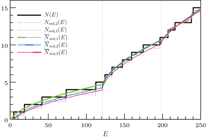
Figure 2: Counting function for a 3-star with $L_{1}=\sqrt{2}$, $L_{2}=\sqrt{3}$, $L_{3}=1$, $V_{1}=0$, $V_{2}=121$, $V_{3}=198$ and Dirichlet conditions at all vertices of degree one. The exact counting function $N(E)$ (fat brown line) is obtained from finding zeros of the secular function. $N(E)_{\mathrm{red},n}$ (dashed lines) gives the trace formula based on a reduced quantum map of dimension $2n$ (for $n=3$ this is the full map, $n=1$ coincides with the exact stair case), and $\overline{N}(E)_{\mathrm{red},n}$ (full lines) gives the ‘mean’ parts of these trace formulas. The latter are plotted fat in the intervals $V_{n-1}<E<V_{n}$ where the corresponding full trace formula is valid and the split into mean part and oscillating part is most natural.

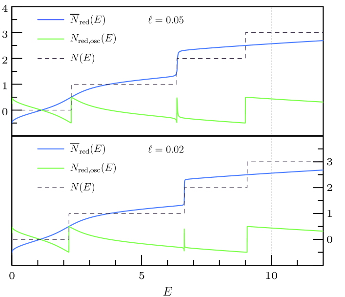
Figure 3: Counting function (mean part $\overline{N}(E)$, oscillating part $N_{\mathrm{osc}}(E)$, and their sum $N(E)$ for a 3-star graph with lengths $L_{1}=1$, $L_{2}=0.5$, $L_{3}=L_{2}+\ell$, $V_{1}=0$, $V_{2}=V_{3}=10$ with Kirchhoff matching conditions at the center, Dirichlet conditions at the end of edge $e=1$ and (attractive) Robin conditions with coupling parameters $\lambda_{2}=\lambda_{3}=-2.5$. All expressions use the reduced approach appropriate for $E<V_{2/3}$. The length mismatch is $\ell=0.05$ in the upper panel and $\ell=0.02$ in the lower panel.

A star graph has one central vertex and $N_{E}=N_{V}-1$ edges that connect the central vertex to dangling vertices of degree one. The above description results in a quantum map $U(E)$ of dimension $2N_{E}\times 2N_{E}$ where each dimension of the map correspond to a directed edge. The simple topology of star graphs implies that a plane wave that moves out from the center is reflected back on the same edge in the opposite direction. As a consequence one often uses an equivalent description using a smaller quantum map $\tilde{U}(E)$ that has dimension $N_{E}\times N_{E}$ where each dimension corresponds to an undirected edge. In this case one may write

$$T=\begin{pmatrix}\tilde{T}&0\\ 0&\tilde{T}\end{pmatrix}$$ (65)

and

$$S=\begin{pmatrix}0&\tilde{\sigma}\\ \sigma^{(N_{E}+1)}&0\end{pmatrix}$$ (66)

where $\sigma^{(N_{E}+1)}$ is the vertex scattering matrix at the center, $\tilde{\sigma}=\mathrm{diag}(\sigma^{(1)},\dots,\sigma^{(N_{E})})$ contains the scalar scattering coefficients at the dangling vertices, and $\tilde{T}=\mathrm{diag}(e^{iK_{1}L_{1}},\dots,e^{iK_{N_{E}}L_{N_{E}}})$ is the diagonal $N_{E}\times N_{E}$ matrix that contains phase factors for traveling along one end to the other on each edge. As the quantum map $U$ has a block form that vanishes on the diagonal one then finds that the secular function may be written as

$$\det\left(\mathbb{I}-U\right)=\det\left(\mathbb{I}-\tilde{U}\right)$$ (67)

with

$$\tilde{U}=\tilde{T}\tilde{\sigma}\tilde{T}\sigma^{(N+1)}=\tilde{\sigma}\tilde{T}^{2}\sigma^{(N+1)}\ .$$ (68)

The matrix $\tilde{U}$ is a quantum map defined on edges rather than directed edges and it describes the scattering on incoming plane waves at the center using $\sigma^{(N+1)}$ followed by propagation along the edges from the center out using $\tilde{T}$, the reflection at the dangling vertices using $\tilde{\sigma}$ and propagation back to the center using $\tilde{T}$. Note that $U$ is unitary if and only if $\tilde{U}$ is unitary.

Our introductory example in Section II can be considered as the simplest incarnation of a star with $N_{E}=2$ edges corresponding to the two sub-intervals and Dirichlet conditions. There we have used the smaller $2\times 2$ description which is more compact but wrote $U$ rather than $\tilde{U}$. For general graph topologies the description has to be based on directed edges and that is what we have sticked to in the rest of the description. For star graphs is is straight forward to translate all results obtained using $U$ in terms of $\tilde{U}$.

To illustrate the theory and, especially, how the trace formula can be applied in practice let us consider a star graph with $N_{E}$ edges and assume Kirchhoff matching conditions at the center (continuity of the wavefunction through the vertex and a vanishing sum over all edges of the outward derivative of the wavefunction at the center). On the dangling vertices of degree one we will put $\delta$-type conditions with coupling parameter $\{\lambda_{e}\}_{e=1}^{N_{E}}$. The latter are also known as Robin-conditions and are defined by $\phi_{e}^{\prime}(L_{e})=\lambda_{e}\phi_{e}(L_{e})$. With $\lambda_{e}\to\infty$ or $\lambda_{e}=0$ this includes Dirichlet or Neumann conditions as special cases. With our introductory example in Section II we have already considered star with $N_{E}=2$ edges corresponding to the two sub-intervals and Dirichlet conditions. For a three-star, $N_{E}=3$ with Dirichlet conditions at all degree one vertices and some arbitrary choice of lengths and potentials one finds similar behavior as for the introductory two-star example, see Figure 2. Apart from having two threshold energies instead of one, we may refer to the discussion in Section II of Figure 1.

One may wonder how the trace formula works when there are eigenstates that vanish exactly on a subgraph with low edge potentials. How can the reduced scattering approach ‘see’ these states? Or are they missed out? For special choices of the parameters and using Robin conditions with negative (attracting) coupling parameters one may consider these questions for a star graph with $N_{E}=3$ edges. To construct such a case, let us choose $V_{1}=0$, $V_{2}=V_{3}>0$, $L_{2}=L_{3}$, $\lambda_{1}\to\infty$ and $\lambda_{2}=\lambda_{3}$ such that the edges $e=2$ and $e=3$ are identical. In that case the eigenstates will either be odd or even under exchange of the two edges and all odd eigenstates will vanish on the edge $e=1$. Choosing Dirichlet conditions everywhere (that is sending $\lambda_{2}=\lambda_{3}$ to infinity) the odd eigenstates can be constructed explicitly as $\phi_{1}(x_{1})=0$, $\phi_{2}(x_{2})=A\sin(n\pi x_{2}/L_{2})$ and $\phi_{3}(x_{3})=-A\sin(n\pi x_{3}/L_{3})$ for some amplitude $A\neq 0$ and positive integer $n$. The corresponding eigenenergies are $E=\frac{n^{2}\pi^{2}}{L_{2}^{2}}+V_{2}>V_{2}$. For finite (positive or negative) values of $\lambda_{2}=\lambda_{3}$ these energies decrease as the coupling parameters are lowered. For Neumann conditions $\lambda_{2}=\lambda_{3}=0$ they have decreased to $E=\frac{(n-1/2)^{2}\pi^{2}}{L_{2}^{2}}+V_{2}>V_{2}$. For negative coupling parameter one may drive the lowest of these energies below the threshold $V_{2}$. As long as the graph is completely symmetric the wavefunction does not leak into the edge $e=1$. Let us consider how this situation may be approached numerically by introducing a small mismatch of the lengths $L_{3}=L_{2}+\ell$. This is the regime shown in Figure 3 where we plot the counting function below the lowest threshold. With the given choice of parameters there are three eigenvalues below threshold. By construction the wavefunction of the central one becomes completely localized on edges $e_{2}$ and $e_{3}$ as $\ell\to 0$. Plotting the mean and oscillating parts as defined by the reduced quantum map of dimension $2\times 2$ one can see that the mean part remains smooth at the lower and upper eigenenergy as $\ell\to 0$ while it develops a discontinuous step at the central energy. At the same time the step in the oscillating part narrows to a tiny resonance at this position (while the steps remain clear for the other two eigenenergies). If one sets $\ell=0$ from the start then the trace formula misses the central eigenenergy: the expressions for smooth and oscillating part are just continuous here. The limit $\ell\to 0$ however creates a step – this is possible due to the multi-valuedness of the complex logarithm. While we have excluded this case by assumption in our derivation, this numerical analysis gives an indication that one may define a trace formula with the reduced quantum map that does not miss out any states that localize in the evanescent part by using continuity with respect to some parameters (lengths, potentials, matching conditions).

VI Outlook

We have expanded the spectral theory of quantum graphs by constructing a scattering approach for quantum graphs with piecewise constant potentials and a multi-mode wave function with a finite number of modes on each edge. In this finite case it is formally sufficient to just consider single-mode quantum graphs with edge-wise constant potentials as one can always map the multi-mode graph to an equivalent larger graph with parallel edges, single-mode wavefunctions and inferred matching conditions. The presence of evanescent modes involves non-unitary scattering matrices as a direct consequence. This is a challenge for the construction of a trace formula for the spectral counting function and we have overcome this challenge by introducing a reduced unitary approach.
The scattering approach for quantum graphs may be used in other settings straight forwardly, e.g. for scattering from a finite (compact) graph with a finite number of leads attached. Many of our constructions are valid beyond quantum graph theory as they build on the generic symmetries of scattering matrices in the presence of evanescent modes – e.g. in the semiclassical scattering approach to quantum billiards where evanescent modes are always present and there is an infinite series of energy thresholds where single evanescent modes become oscillatory.
Finally, in a way the trace formula we have presented is not quite complete. We have assumed that the energy is always larger than the lowest edge potential. But how do we count the number of states below the lowest potential. The reduced scattering matrix has zero dimension, so the approach does not seem to make immediate sense. We leave this open for further investigation.

Appendix A Multi-mode quantum graphs and their formal equivalence to a single-mode quantum graph

Let us consider the MM setting on a connected metric graph with $N_{V}$ vertices and $N_{E}$ edges. In this setting the scalar wavefunction $\phi_{e}(x_{e})$ on the edge $e$ is replaced by a multi-component wavefunction

$$\boldsymbol{\phi_{e}}(x_{e})=\begin{pmatrix}\phi_{e,1}(x_{e})\\ \dots\\ \phi_{e,\mu_{e}}(x_{e})\end{pmatrix}$$ (69)

with $\mu_{e}$ components and a Schrödinger operator $\hat{H}$ acts on a given edge as

$$\left(\hat{H}\boldsymbol{\Phi}\right)_{e}=-\frac{d^{2}\boldsymbol{\phi_{e}}}{dx_{e}^{2}}(x_{e})+\boldsymbol{V}_{e}\boldsymbol{\phi_{e}}(x_{e})$$ (70)

where diagonal (constant) matrix $\boldsymbol{V}_{e}=\mathrm{diag}\left(V_{e,1},\dots,V_{e,\mu_{e}}\right)$ replaces the scalar potential. We will always assume that the number of modes $\mu_{e}$ is finite on each edge but we do allow $\mu_{e}<\infty$ to vary from one edge to another. By straight forward extension of schrader matching conditions that render the corresponding Schrödinger operator $\hat{H}$ self-adjoint follow the same pattern as in the single-mode case. At a given vertex $v$of degree $d_{v}$ one may write the matching conditions as linear relations between the adjacent multi-component wavefunctions and their derivatives

$$\sum_{e^{\prime}}\left(A_{ee^{\prime}}\boldsymbol{\phi}_{e^{\prime}}(0)+B_{ee^{\prime}}\frac{d\boldsymbol{\phi}_{e^{\prime}}}{dx_{e^{\prime}}}(0)\right)=0$$ (71)

where the sum is over all edges $e^{\prime}$ adjacent to $v$ and there are $d_{v}$ – one for each adjacent edge $e$. The coefficients $A_{ee^{\prime}}$ and $B_{ee^{\prime}}$ are now matrices of size $\mu_{e}\times\mu_{e^{\prime}}$. Let $\tilde{d}_{v}=\sum_{e=1}^{d_{v}}\mu_{e}$ (the number of all modes on adjacent edges) then we can combine the coefficient matrices to a large matrix of size $\tilde{d}_{v}\times\tilde{d}_{v}$ and the linear relations define a self-adjoint problem if and only if $AB^{\dagger}=BA^{\dagger}$ is a hermitian matrix and that the $\tilde{d}_{v}\times 2\tilde{d}_{v}$ matrix $(A,B)$ has maximal rank $\tilde{d}_{v}$. If $\mu_{e}=1$ on all edges our description of a multi-mode graph reduces to a single-mode quantum graph with constant potentials as a special case. However we may also view a multi-mode graph with $N_{V}$ vertices with degrees $\{d_{v}\}_{v=1}^{N_{V}}$ and $N_{E}=\frac{1}{2}\sum_{v=1}^{N_{V}}d_{v}$ edges with $\{\mu_{e}\}_{e=1}^{N_{E}}$ modes as a single-mode PCP quantum graph with the same number of vertices $N_{V}$ and $\tilde{N}_{E}=\sum_{e=1}^{N_{E}}\mu_{e}=\frac{1}{2}\sum_{v=1}^{N_{V}}\tilde{d}_{v}$ single-mode edges by replacing each edge $e$ in the original multi-mode graph by $\mu_{e}$ parallel edges of the same length $L_{e}$ with single-mode wave functions $\phi_{e,m}(x_{e})\mapsto\phi_{e,m}(x_{e.m})$ (where $x_{e,m}$ with $1\leq m\leq\mu_{e}$ is the coordinate on the $m$-th parallel edge). The excitation energies $V_{e,m}$ ($1\leq m\leq\mu_{e}$) then become constant potentials on the $m$-th parallel edge and the description of self-adjoint matching conditions carries over in a natural way. In the rest of the paper we will use the formal language of single-mode PCP quantum graphs and think of MM quantum graphs as a special case with parallel edges of the same length. While this equivalence between the MM and PCP picture on an enlarged graph is formal it is straight forward to adapt in a theoretical setting as well as practically in an experiment. In the former one may prescribe matching conditions and excitation energies as required and in the latter the relevant parameters can be measured (or chosen consistently with available measurements).

References

- (1) J.-P. Roth, Spectre du laplacien sur un graphe, C.R.Acad.Sci. Paris Sér. I Math. 296, 793–795 (1983).
- (2) T. Kottos, U. Smilansky, Quantum Chaos on Graphs, Phys. Rev. Lett. 79, 4794 (1997).
- (3) S. Gnutzmann, U. Smilansky, Quantum graphs: Applications to quantum chaos and universal spectral statistics, Advances in Physics 55,527 (2006).
- (4) G. Berkolaiko, P. Kuchment, Introduction to Quantum Graphs (AMS, Providence, 2013).
- (5) O. Hul, S. Bauch, P. Pakoński, N. Savytskyy, K. Życzkowski, L. Sirko, Experimental simulation of quantum graphs by microwave networks, Phys. Rev. E 69, 056205 (2004).
- (6) M. Allgaier, S. Gehler, S. Barkhofen, H.-J. Stöckmann, U. Kuhl, Spectral properties of microwave graphs with local absorption, Phys. Rev. E 89, 022925 (2014).
- (7) A. Rehemanjiang, M. Allgaier, C.H. Joyner, S. Müller, M. Sieber, U. Kuhl, H.-J. Stöckmann, Microwave realization of the gaussian symplectic ensemble, Phys. Rev. Lett. 117, 064101 (2016).
- (8) B. Dietz, V. Yunko, M. Białous, S. Bauch, M. Ławniczak, L. Sirko, Nonuniversality in the spectral properties of time-reversal-invariant microwave networks and quantum graphs, Phys. Rev. E 95, 052202 (2017).
- (9) Z. Fu, T. Koch, T.M. Antonsen, E. Ott, S.M. Anlage, Experimental Study of Quantum Graphs with Simple Microwave Networks: Non-Universal Features, Acta Physica Polonica A, 132, 1655 (2017).
- (10) A. Johnson, M. Blaha, A.E. Ulanov, A. Rauschenbeutel, P. Schneeweiss, J. Volz, Observation of Collective Superstrong Coupling of Cold Atoms to a 30-m Long Optical Resonator Phys. Rev. Lett. 123, 243602 (2019).
- (11) M. Ławniczak, P. Kurasov, S. Bauch, M. Białous, V. Yunko, L. Sirko, Hearing Euler characteristic of graphs, Phys. Rev. E 101, 052320 (2020).
- (12) P. Exner, H. Kovarik, Quantum Waveguides, (Springer, Chams, 2015).
- (13) O. Post, Spectral Analysis on Graph-like Spaces (Springer, Berlin, 2012).
- (14) H.A. Weidenmüller, Studies of Many-Channel Scattering, Annals of Physics 28, 60-115 (1964).
- (15) H. Schanz, U. Smilansky, Quantization of Sinai’s billiard – a scattering approach, Chaos, Solitons & Fractals 5, 1289-3009 (1995)
- (16) C. Rouvinez, U. Smilansky, A scattering approach to the quantization of Hamiltonians in two dimensions – application to the wedge billiard, J. Phys. A 98, 77-104 (1995).
- (17) C. Brewer, S.C. Creagh, G. Tanner, Elastodynamics on graphs – wave propagation on networks of plates, J. Phys. A 51, 445101 (2018).
- (18) V. Kostrykin and R. Schrader, Kirchhoff’s Rule for Quantum Wires, J. Phys. A 32, 595 (1999).
- (19) P. Kuchment, Quantum Graphs I. Some basic structures, Waves in Random media 14, S107 (2004).
- (20) U. Smilansky, Irreversible quantum graphs, Waves in Random Media 14, S143 – S153 (2004); M. Solomyak, On a differential operator appearing in the theory of irreversible quantum graphs, Waves in Random Media 14, S173-S185 (2004); U. Smilansky, M. Solomyak, The quantum graph as a limit of a network of physical wires, Contemporary Mathematics 415, 283-292 (2006).
- (21) J. Bolte, S. Endres, The Trace Formula for Quantum Graphs with General Self Adjoint Boundary Conditions, Ann. H. Poincaré 10, 189 (2009).