A Scalable Solution for Running Ensemble Simulations for Photovoltaic Energy

Abstract

This chapter proposes and provides an in-depth discussion of a scalable solution for running ensemble simulation for solar energy production. Generating a forecast ensemble is computationally expensive. But with the help of Analog Ensemble, forecast ensembles can be generated with a single deterministic run of a weather forecast model. Weather ensembles are then used to simulate 11 10 KW photovoltaic solar power systems to study the simulation uncertainty under a wide range of panel configuration and weather conditions. This computational workflow has been deployed onto the NCAR supercomputer, Cheyenne, with more than 7,000 cores.

Results show that, spring and summer are typically associated with a larger simulation uncertainty. Optimizing the panel configuration based on their individual performance under changing weather conditions can improve the simulation accuracy by more than 12%. This work also shows how panel configuration can be optimized based on geographic locations.

1 Introduction

The reliance on fossil fuels for power generation is not sustainable for meeting the increasing demand of a growing global economy and population. Building a sustainable society requires alternative sources for power production that can last for generations to come [1]. Thanks to new incentives, regulations, improvements in technology, development of a competent workforce, paired with a general shift in sentiment against pollution and greenhouse emissions, renewable sources account for a significant portion of the overall energy production portfolio.

In 2019, for the first time in history, more energy in the U.S. was produced from renewable sources than from coal [2]. Since early 2000s, the general trend of energy production in the U.S. showed a steady decline in coal, offset by an increase in natural gas, and renewable sources. Predictions by the U.S. Energy Information Administration (EIA) for 2050 suggest that 36% of energy will be generated using natural gas (37% in 2019), 38% from renewables (19% in 2019), 12% nuclear (19% in 2019), and only 13% from coal (24% in 2019) [3]. Therefore, while natural gas is predicted to remain almost constant over the next 30 years, renewable will double to offset coal and nuclear power. Specifically, it is projected that solar generation will account for almost 80% of the increase in renewable generation through 2050 [4].

Relying on solar power, however, can be challenging, despite the massive progress in utility-scale installation and the prevalence of residential Photovoltaic (PV) systems among communities. The sheer amount of available solar power does not necessarily guarantee its full utilization and integration into our electricity grid. This is due to rapidly changing weather conditions, astronomical factors, and other events that alter the amount of power produced. In general, it can be said that there is a greater uncertainty associated with generating power using PV because external weather conditions play a dominant effect.

The key challenging problem is to match power production with demand, both of which are dynamic and variable. Furthermore, this must occur at different time-scales, ranging from day-ahead to seconds.

In the U.S. and most other countries, the energy production planning occurs in what is referred to as a day-ahead market [5]. Each day, a portfolio of energy sources is created to meet a predicted demand. A bidding process sets the price of electricity, where the different producers offer to sell electricity at a specific price. Generally speaking, if a producer offers to sell a certain amount of energy at a price, not meeting the specific amount incurs in a penalty, and generating more energy leads to an opportunity loss [6, 7]. This process favors energy sources with smaller day-ahead uncertainty.

Traditional fossil fuel power sources, and some types of renewables such as hydroelectric power, have little day-ahead uncertainly, because the amount of potential power generation is directly proportional to the fuel available, may this be stored natural gas or volume of water in a reservoir. On the other hand, PV solar energy has larger uncertainty due changing weather conditions, astronomical factors, technological constraints, operational practices.

Weather: Numerical Weather Prediction (NWP) are used to forecast day-ahead irradiance, which depends on general weather conditions [8]. While they are effective, they are also error prone, especially in case of rare or extreme events. For example, clouds [9, 10] and precipitation are an important factor that changes the amount of solar irradiance reaching solar panels, but their day-ahead modeling is difficult, and often requires multiple parameterization schemes. Similarly, aerosols interact with the incoming solar irradiance [11, 12] by increasing the diffused component of insolation. Any changes in irradiance, which can either decrease or sometimes increase, leads to an additional uncertainty in power production. Aerosols are present in larger quantities and thus have stronger impact in areas with heavy air pollution, and transient events like desert storms or volcanic eruptions. Because of the uncertainty in weather forecasts, it is currently not possible to always and consistently forecast day-ahead PV solar energy production.

Astronomical: Additionally, PV solar energy is not available during the night, and daytime production changes throughout the year depending on sunrise and sunset times, and solar elevation. While this variability can be easily forecasted and accounted for, it still requires a daily optimization to properly estimate future energy production.

Technological: Another source of uncertainly is intrinsically related with the electro-chemical processes that PV panels rely upon to generate electricity. The efficiency of power generation varies based, in addition to irradiance, also on cell temperature [13, 14], which itself is related to ambient temperature. Wind speed affects air temperature, and thus must be taken into account to make accurate predictions [15, 16]. Once irradiance and temperature are forecasted, the conversion to power generation can be made through a PV panel simulator. However, the nominal panel power capacity is evaluated under Standard Test Condition (STC), which might be different than real-world performance. For example, the STC specifies a cell temperature of 25°C and an irradiance of 1000 $W/m^{2}$ with an air mass 1.5 spectrum. These conditions are only rarely if ever met.

Operational: Finally, panels must be maintained clean and they generally degrade with time, leading to their efficiency changing constantly. Given two identical weather conditions, the same panel might generate a different amount of electricity at different times.

1.1 Solar Power Forecasting

Solar power forecasting can be viewed as a two-step problem: characterizing the weather and the PV panels. There are many different methods to solve these two problems, sequentially or concurrently, and they depend on factors such as the temporal and spatial scale of the results, the temporal resolution, if a measurable level of uncertainty is required, and the computational resources available.

Solar power forecasting is usually divided based on the temporal forecasting horizon [17]. Forecasting up to six hours is referred to as short-term, and it is where extrapolation and persistence methods excel due to their computational efficiency and good accuracy [18]. Following, is mid-term forecasting, spanning from six to 72 hours, where physical and/or statistical numerical modeling is considered the most effective technique. Because of the rapidly changing environmental conditions, the immediate ambient history of is not a good predictor for future outcomes.

For day-ahead mid-term forecasts which are the focus of this research, the weather part is solved using NWP models, that resolve weather features and forecast future conditions (e.g., cloud cover, wind speed, temperature). They are run at different temporal and spatial scale, and can be optimized for specific locations and weather patterns. However, weather forecasts do not directly translate into amount of power generated, and specific characteristics of the PV array and its installation, as well as operational status, must be taken into account.

The second step can be solved using solar panel numerical simulators or simple empirical functions; or using statistical and computational methods based on past measurements. Which method to use is dictated by the specific needs and the level of accuracy required, but in general it can be said that simulators are less effective at accounting for the specific aspects of installation and location, while statistical and computational solutions are limited to historical patterns which might under-represent conditions, most importantly, rare or extreme events. The latter methods can also only be used in the presence of a robust history of measurements, and thus are generally unsuitable for feasibility studies. The results are also very location dependent, and while they might be optimal at predicting a specific panel configuration and installation, their results are likely to be so specific that cannot be generalized to other locations or installations. Finally, because panels degrade over time, a statistical correction is also needed to capture this decrease in efficiency.

Among the statistical and computational methods, Artificial Neural Network (ANN) have been used to predict both the behavior of panels, and in some cases also the weather conditions. A plethora of literature [16, 18, 19, 20, 21, 22, 23, 24, 25, 26] have emerged to study the application of ANN on solar power forecasting because they can be trained to focus on a geographically confined region and optimize local solar power forecasting. The general idea is to train an ANN to learn the statistical pattern between weather variables and the observed power production. This technique usually requires a historical archive of weather observations together with the associated power production records. A properly trained ANN is able to model the condition of solar panels and the surrounding environment like shadowing.

1.2 Quantification of Uncertainty

The simulation of a power production system is a highly complex and volatile process. Uncertainty arises when a complete and exact information on a process is lacking.

To simulate the amount of power generated, information regarding the weather (solar irradiance and temperature) and the panel (installation and condition) are needed. However, both are subject to a lack of information, and therefore, uncertainty. The atmosphere is a chaotic system that cannot be precisely observed and as a result, “the prediction of the sufficiently distant future is impossible by any means” [27]. Observations often have limited spatio-temporal resolution and NWP models only approximate the true physical processes and atmospheric interactions.

With regards to the simulation of panel performance, uncertainty can originate from an imprecise representation of the surrounding environment, e.g. shadowing, and from an incomplete characterization of real world performance under a wide range of possible weather conditions, since the panels are typically tested under the STC.

Simulation ensembles are particular helpful in quantifying uncertainty in the forecasts. In weather forecasting, NWP models can be run many times to generate a range of possible deterministic realizations of the future state of the atmosphere. This ensemble of possible future states provides a quantifiable representation of the uncertainty for a given forecast. If ensemble members are very different, referred to as ensemble spread, the specific uncertainty for the forecast is high.

There are many approaches for constructing a forecast ensemble, for example, applying varying perturbations applied to initial state variables (i.e. wind speed, temperature), changing dynamics schemes or parameterizations of an NWP model, or using stochastic means for perturbing physical parameterizations [28, 29]. A hybrid approach can also be devised by combining one or more of the aforementioned methods. However, these approaches involve running NWP models multiple times, which is computationally expensive.

The analog-based approach, Analog Ensemble (AnEn), has been proposed [30] to construct forecast ensemble without extra runs of NWP models. The AnEn is a technique to generate forecast ensembles with a deterministic NWP model and the corresponding historical observations. It does not require extra runs of the deterministic model which already offers a great reduction in the computational cost of ensemble generation. It has been successfully applied to a series of forecasting problems, including surface variables [30, 31, 32, 33] and renewable energy production [34, 8, 35, 23, 36]. An in-depth introduction on the AnEn is provided in Section 3.1.

1.3 Scope and Organization

This chapter introduces a scalable workflow that focuses on evaluating solar power production and its predictability from geographically diverse regions. Instead of relying on ground observations, a NWP model is coupled with a PV solar power simulation system which tests the predictability of 11 different PV modules. These PV modules vary in many aspects including material, size, and efficiency.

Power forecasts are generated by using an AnEn ensemble of NWP forecasts that characterize future weather conditions, where each member of the ensemble is used as input for the panel simulator. Therefore, for any given day 21 weather conditions are each used to generate 11 power predictions, where 21 is the size of the weather ensemble and 11 is the number of the panel configurations. This is repeated for every grid over Continental United States (CONUS) ( 60,000) every hour for the daylight time of the day for 2019, leading to over 60 trillion computations. The system is verified by using the analysis fields of the weather model, which is the closest complete and high resolution geographical estimation of real-world weather conditions.

Results show that PV modules have various levels of predictability and they should be chosen based on optimizing both the power production and the predictability to support solar energy penetration. This workflow is designed to be scalable because of the very large number of computations required, which can scale significantly if testing more panel configurations, or increasing further the spatial and temporal scope or their resolutions.

The rest of the chapter is organized as follows: Section 2 introduces the research data used in this project; Section 3 describes the main methodology of generate ensemble forecasts with the Parallel Analog Ensemble (PAnEn) implementation [37] and its integration with a power simulation system implemented with PV_LIB [38]; Section 4 shows results for solar power simulation with a total of 11 PV modules; Section 5 specifically discusses the design of the scalable workflow with the RADICAL Ensemble Toolkit (EnTK) [40]; and finally, Section 6 summarizes the chapter.

2 Research Data

2.1 The North American Mesoscale Forecast System

The North American Mesoscale Model (NAM) is a weather forecast model operated by the National Centers for Environmental Prediction (NCEP). It aims to provide short-term deterministic forecasts for weather variable at a variety of vertical levels and on multiple nested domains. Currently, the Weather Research and Forecasting (WRF) Nonhydrostatic Mesoscale Model (NMM) is run as the core of NAM after its replace of the Eta model in 2006, and since then, the three names are interchangeable, NAM, WRF, and NMM, typically referring to the same model output.

NAM is initialized four times per day at 00, 06, 12, and 18 UTC. It is run with multiple nested domains with differences in the geographic coverage and the spatio-temporal resolution. In this study, the parent domain (NAM-NMM) with a 12 km spatial resolution is used. This domain covers North America. The production run provides forecasts up to 84 hours into the future, namely an 84-hour Forecast Lead Time (FLT), with the first 36 hours being hourly and the rest of the lead times being every 3 hours. The parent domain run is initialized with a 6-hour Deep Analog (DA) cycle and it is updated hourly using the hybrid variational ensemble Gridpoint Statistical Interpolation (GSI) and the NCEP Global Ensemble Kalman Filter method. The analysis production is usually referred to as NAM-ANL. There are other one-way nested domains within the parent 12 km domain, e.g., CONUS, Alaska, Hawaii, and Puerto Rico. These nested domains have a fixed 3 km spatial resolution and a 60-hour FLT. However, only the parent grid products have a historical data archive since 2006 available from NCEP.

In this study, NAM-NMM initialized at 00Z and NAM-ANL initialized at 00, 06, 12, and 18 UTC, are collected between 2017 and 2019. Since the day-ahead PV energy market is of particular interest and CONUS covers four time zones, the FLT s from 06Z to 32Z from NAM-NMM are focused on throughout the study. This lead time period covers from 01:00 (the day of initialization) to 03:00 (the next day) in the Easter time zone, and from 22:00 (the day prior to initialization date) to 00:00 (the next day) in the Pacific time zone. There is no compensation for day-light saving when calculating the local time to simplify the computation and analysis. NAM provides a few hundred variables. Table 1 summaries the variables used in this study.

Table 1: Variables from NAM-NMM and NAM-ANL used in this study

Variable Short name Unit Vertical level Downward short-wave radiation flux dswrf $W/m^{2}$ Surface Albedo al $\%$ Surface Pressure sp $Pa$ Surface Orography orog $m$ Surface Temperature 2t $K$ 2 m above ground U wind component 10u $m/s$ 10 m above ground V wind component 10v $m/s$ 10 m above ground Total Cloud Cover tcc $\%$ Atmosphere as a single layer

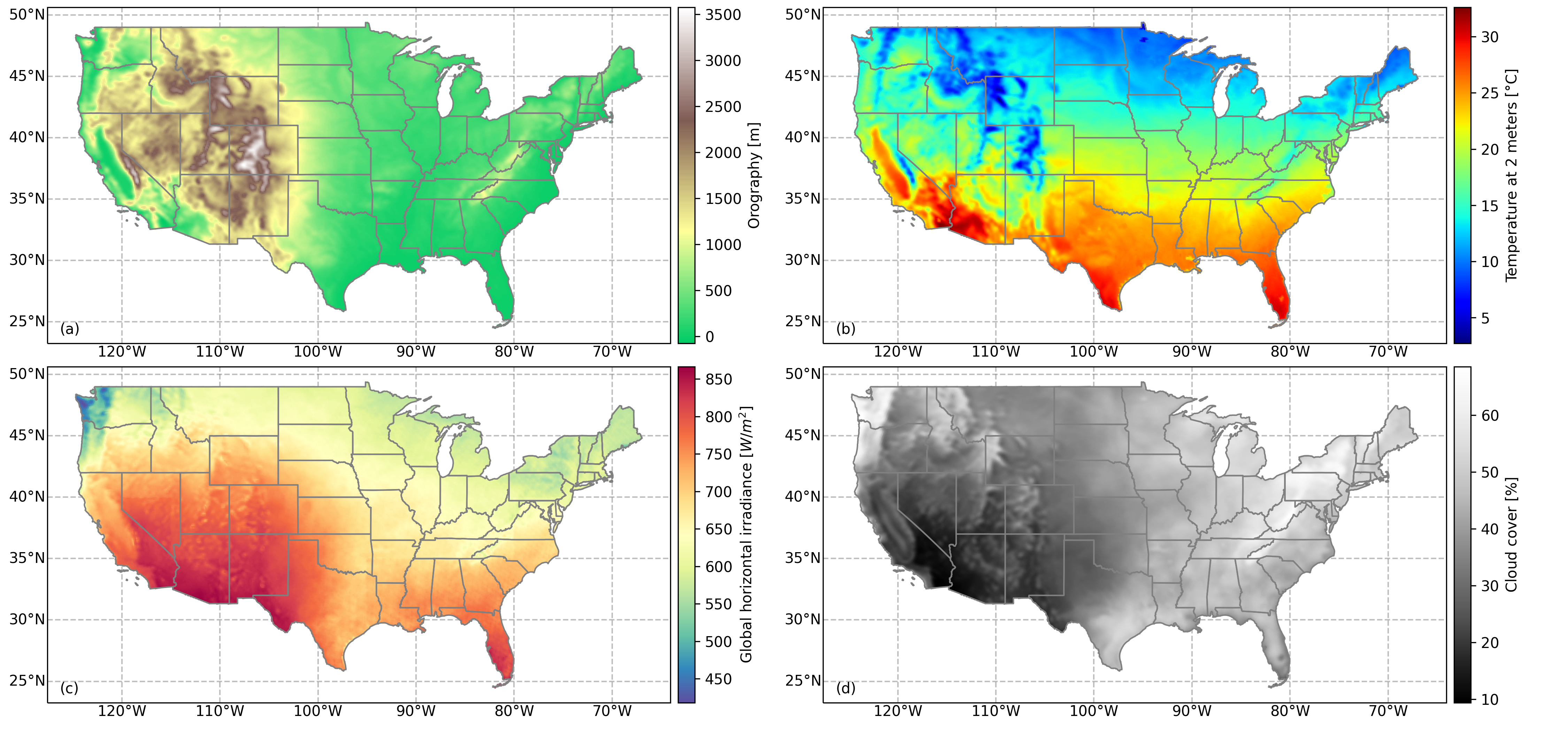
Figure 1: NAM-ANL over CONUS for 2018: model orography (a), average daily maximum temperature at 2 meters (b), average daily maximum GHI (c), and average cloud cover (d). State boundaries are shown in solid lines.

Figure 1 shows the NAM orography in (a) and the annual average of daily maximum temperature, daily maximum GHI, and cloud cover respectively in (b, c, d) for 2018. The terrain representation of NAM is aggregated from a high resolution U.S. Geological Survey (USGS) 30’ elevation dataset. The horizontal resolution of the USGS 30’ dataset is about 0.6 km at 40°N. The elevation of the center of each individual NAM grid cell is set to the average elevation of the area in the USGS dataset. A smoothing operation has been originally carried out to reduce the level of noise in the high resolution elevation dataset. As shown in Figure 1a, the model orography reflects well the elevation variation at and west to Rocky Mountains and at Appalachian Mountains. The spatial features of Coastal Ranges are also legible from the map. CONUS has complex terrain features with elevation ranging from -74 m to 3577 m. Figures 1b, c show the annual average of daily maximum temperature and GHI respectively. Daily maximum, instead of average, are calculated from the hourly analysis field. This is to avoid skewing the statistics by including night times of which are not of particular focus. Surface temperature exhibits typical longitudinal patterns with exceptions to region regions with drastic topographic changes. GHI has a strong correlation with temperature, exhibiting higher levels at Rocky Mountains, the Great Basin, and Coastal Plains near Florida, compared to the other regions. Adversely, Coast Ranges at west Washington and west Oregon has a low level of annual GHI. This can be explained by the annual average of cloud cover, as shown in Figure 1. Significant cloud cover is observed near these regions, blocking the incoming solar radiation. Cloud cover is one of the governing parameter for GHI, and therefore, they are highly correlated. In terms of PV power production, however, ambient temperature also plays an important factor because it affects the temperature of PV panel module cells which, in turn, affects the efficiency of power generation.

2.2 IECC Climate Zones

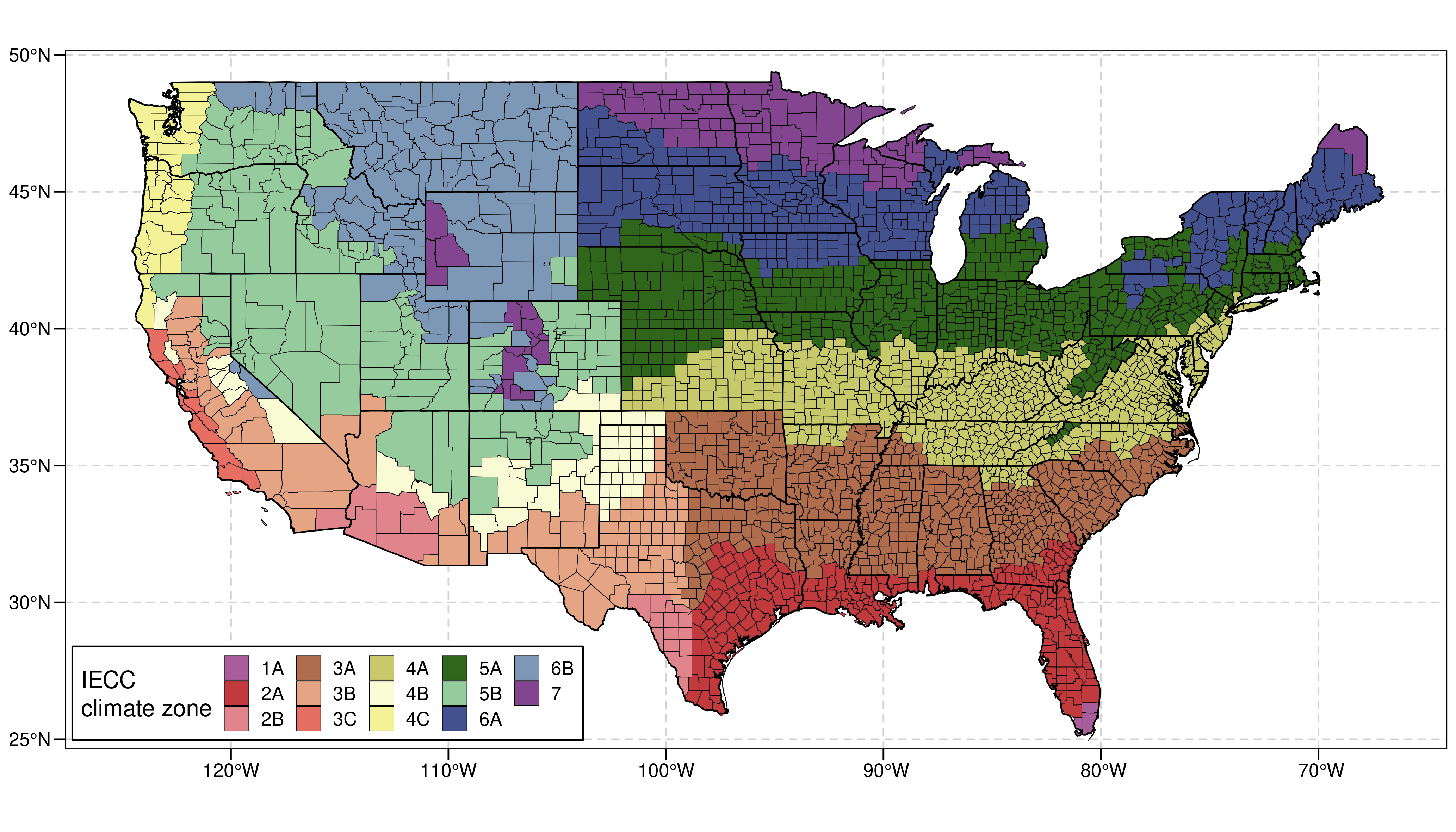
Figure 2: Geographic distribution of climate zones. State and county boundaries are outlined by solid black lines. The letters A, B, and C stand for moist, dry, and marine regions. The numerical numbers from 1 to 8 generally correspond to areas in need of more cooling (being hot) to more heating (being cold).

It is important to evaluate and compare power production and the predictability under different climatological conditions. This study adopts the climate zones defined in the International Energy Conservation Code (IECC) as the criterion to determine clusters within CONUS. IECC is a set of building codes define by the International Code Council, funded by the U.S. Department of Energy. It’s main purpose is to establish the minimum design and construction requirements for energy efficiency. It assigns codes at a county level, and the code typically consists of two part, a numeric digit and a letter. The number is determined based on the thermal criteria which is the accumulated daily temperature anomaly from a predefined temperature threshold. Codes from 1 to 8 typically correspond to places from being very hot (in need of cooling) to being very cold (in need of heating). The other part of the code consists of either A, B, or C, corresponding the major climate types of moist, dry, and marine types. These classification considers both the temperature and precipitation. In the case of CONUS U.S., thermal conditions changes longitudinal while climate types generally change latitudinally.

3 Methodology

PV energy production is closely coupled with meteorological conditions (in particular GHI and temperature) and solar panel configuration (panel type, location, health and installation). A complete predictability assessment of the PV energy production essentially needs to examine both the meteorological factors from weather forecasting and the engineering factors from solar panel performance. This section introduces the framework designed for assessing the large scale predictability of PV energy production with the multivariate AnEn and a simulated performance system.

3.1 Analog Ensemble and the Extension to Multivariate Forecasts

Ensemble simulation is an effective approach to assess the predictability of a weather process. However, generating a forecasting ensemble is computationally expensive. It usually involves multiple model runs, each of which can already take up significant computational resources. The AnEn is a technique to generate forecast ensembles relying on a single run of a deterministic model and the historical observations. It is an efficient solution to ensemble generation because it saves extra simulations required by multi-initialization or multiple models. It is parallelizable and scalable because of the independent ensemble generation at an individual time and place. An in-depth description of how AnEn works in provided below.

The AnEn generates forecast ensembles based on the assumption that similar weather forecasts exhibit similar biases, and by using the observation, these biases can be corrected within an ensemble. The most important component of the AnEn is a forecast similarity metric [30], defined using the following equation,

$$\left\|F_{t},A_{t^{\prime}}\right\|=\sum_{i=1}^{N}\frac{\omega_{i}}{\sigma_{i}}\sqrt{\sum_{j=-\tilde{t}}^{\tilde{t}}\left(F_{i,t+j}-A_{i,t^{\prime}+j}\right)^{2}},$$ (1)

where $\left\|F_{t},A_{t^{\prime}}\right\|$ represents the distance, or the dissimilarity, between a multivariate deterministic target forecast, $F_{t}$, at time $t$, and an analog forecast, $A_{t^{\prime}}$, at a historical time $t^{\prime}$. The right side of the equation is a weighted normalized average of the differences from each predictor variable. $N$ is the number of predictor variables; $\omega_{i}$ is the weight associated with the predictor $i$; and $\sigma_{i}$ is the standard deviation, as a normalizing factor, for the predictor $i$. $F_{i,t+j}$ is the target forecast at time $t+j$ for the predictor $i$ and similarly, $A_{i,t^{\prime}+j}$ is the historical analog forecast at time $t^{\prime}+j$ for the predictor $i$. Finally, $\tilde{t}$ is the half size of the temporal window for trend comparison. This parameter is devised to consider the forecast similarity within a small time window, rather than just at a particular time point, to improve the quality of identified weather analogs. In practice, the half size of the time window is usually set to 1 hour, meaning values from the previous, the current, and the next hours will be compared during the calculation of dissimilarity at the a current time point.

For AnEn to work properly, a set of forecasts and the corresponding observations are required to start with. The time period of the data is usually two years or longer, with at least one year as the historical period, namely the search repository, and the rest of the time as the forecast period, namely the test period. At least one year of data in the search repository is needed to account for seasonal and annual variations and to ensure good weather analogs can be found. This requirement of the length of the historical archive is much shorter than other analog-based forecasting techniques [41, 42] because, with the AnEn, weather analogs are identified within a highly restricted spatial location, independently at each grid point, and a short period of time, usually a few hours. As a result, the degree of freedom of how forecasts can differ from each other is largely constricted both in space and time, making it easier for to identify weather analogs. But the generality still holds true where better weather analogs can be found given a longer search repository.

A slightly different setting of the search and test datasets for AnEn is called the operational AnEn. In this setting, the size of the search repository is not fixed. Rather, it is growing by incorporating forecasts from the test dataset as soon as the target forecast becomes historical. In other words, each target forecast in the test dataset has a different length of search history that incorporates all immediate historical forecasts. This alternative setup helps in cases where only a limited length of search history is available.

After forecast analogs have been identified for a particular target forecasts, the AnEn constructs the final ensemble by directly using the observations associated with the forecast analogs since the forecast analogs are identified from the historical archive. The historical observations compose the AnEn forecast ensemble. This process is repeated for all geographic locations, all target forecasts in the test dataset, and all forecast lead times to generate the complete set of forecast ensembles. In fact, this process is highly parallelizable and scalable because the ensemble generation of forecasts is independent in space and time. The workload can, thus, be “embarrassingly” parallelized with low communication overhead [23, 37].

While the spatial and temporal independence brings great advantages in computation, however, it leads to inconsistent and sometimes unrealistic predictions when ensemble members are analyzed individually [43, 36]. This is because the first member in the forecast ensemble at location $i$ might not necessarily be related to the first member in the forecast ensemble at a nearby location, say $i+1$. The generation of these two ensembles are independent. The member rank follows a pure statistical process of determining the distance between the target and the analog forecasts, rather than any physical linkages or processes. As a result, plotting a geographic map using the first member from ensembles at a particular day leads to patchy and unrealistic features. This problem can be well addressed by using a form of summarization of ensemble members, e.g., the mean or the median. If the ability to analyze each ensemble member is truly desired, the AnEn members need to be shuffled with the Schaake Shuffle (SS) technique [44, 45, 43, 46]. Ensemble spread and standard deviation can be calculated if the uncertainty of ensembles are to be evaluated. A kernel function can also be applied to the AnEn members to construct the Probability Distribution Function (PDF) for probabilistic forecasts. In practice, AnEn forecast ensembles are usually analyzed in its deterministic or the probabilistic forms, rather than on the individual member in space and time.

The AnEn technique for predicting a univariate target has been well studied under the presumption that observations of the variable are available. This scheme does not apply when using the AnEn to generate forecasts for initializing the PV power simulation because the power simulation depends on multiple variables, including GHI, temperature, wind speed, and albedo. Simplistically, one would argue that multivariate forecasts can be generated by running the AnEn multiple times with each generation focusing on one variable at a time. However, this argument does not stand because each AnEn generation is independent and thus, the multivariate forecasts will again suffer from having inconsistent and unrealistic predictions in space and time. In this case, the SS does not help because it is developed for single run of AnEn.

In this study, we propose the multivariate AnEn and extend the application of AnEn to multivariate forecasts with a single pass of the AnEn technique. The multivariate AnEn still relies on the same similarity metric, as defined in Equation (1), to identify analog forecasts for target forecasts. After analog forecasts have been selected, the multivariate ensemble generation shares the same set of analog forecasts. This constrains the degree of freedom when generating multivariate AnEn forecasts in a way that the multivariate AnEn forecasts are only possible if they have been observed as a whole in the past.

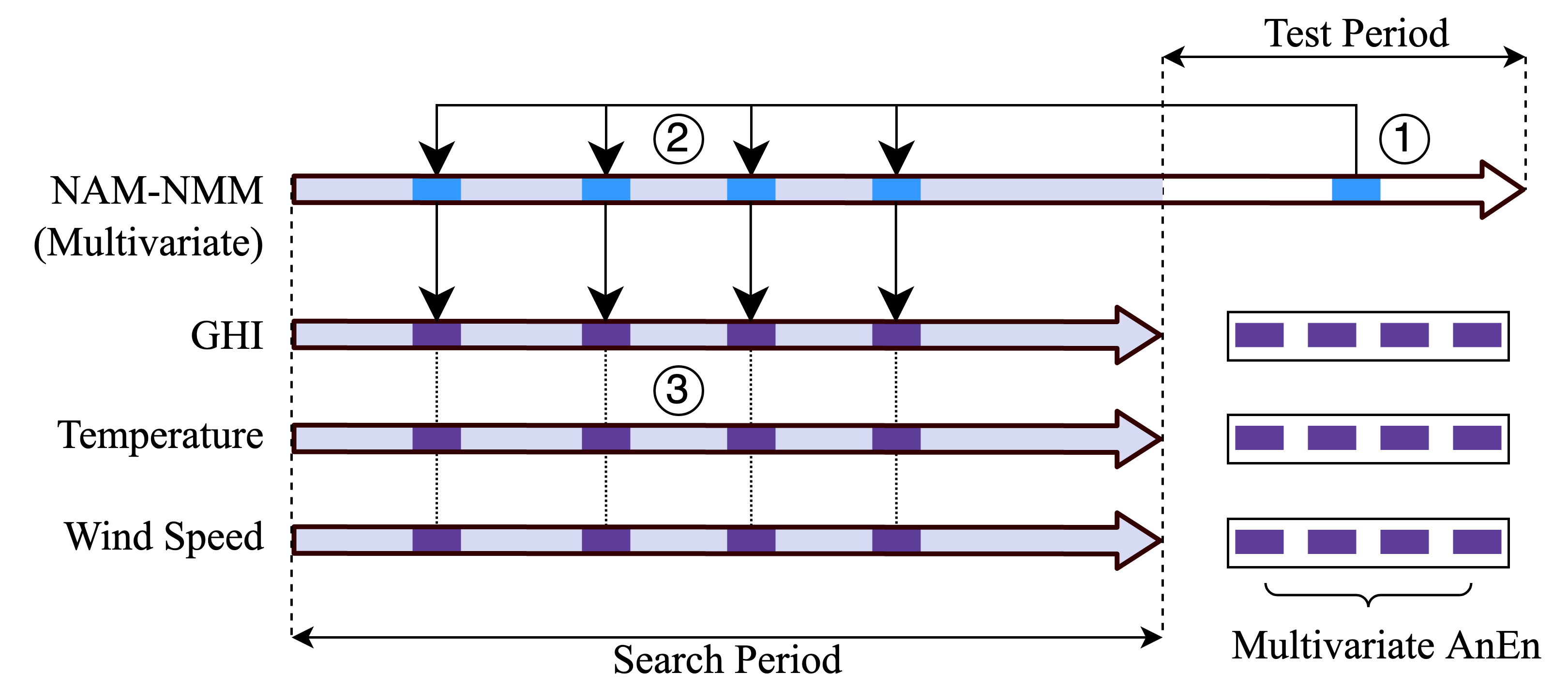
Figure 3: The schematic diagram for generating a four-member multivariate AnEn

Figure 3 shows the schematic diagram for generating a four-member multivariate AnEn. Forecast and observation datasets are represented as a directed arrow to indicate that their sizes might be variable, e.g., as in the operational AnEn. The horizontal direction represents time and it is divided into the search period (as shown in grey) and the test period (as shown in white). The first arrow on from the top represents the NAM-NMM and by the AnEn convention, it is a multivariate deterministic forecasts (recall the parameter $N$ in Equation (1)). The other three arrows below represent three observation datasets that are aligned within and with the time series of NAM-NMM. The algorithm is described below:

1. A multivariate forecast from the test period is selected for which analog forecasts are desired;

2. Four historical forecasts from the search period with the highest similarity (the shortest distance) are identified;

3. The associated observation values are retrieved from a particular observation dataset to form the forecast ensemble. This process is repeated for all the available observation datasets until a complete set of multivariate AnEn has been generated.

The parameterization of the multivariate AnEn stays the same with the univariate AnEn, e.g., having an 1-hour window half size and favoring a longer search period, with one exception for predictor weights. Usually, predictor weights can be optimized based on an error metric of the variable of prediction, namely the predictand, e.g., the Root Mean Square Error (RMSE) or the Continuous Rank Probability Score (CRPS). But the optimization objective is slightly different in the case of the multivariate AnEn because each predictand might be associated with a different set of optimized weights if only conditioned on the individual predictand. In other words, weights for predicting GHI could be very different from weights for predicting wind speed. We, therefore, evaluate the performance of predictor weights based on the forecast error of the final product, the simulated PV power production, by running an power simulation system with the AnEn forecasts.

3.2 Scalable Ensemble Simulation for Photovoltaic Energy Production

The most critical parameter for PV power simulation is GHI, which captures cloud coverage and precipitation, while the power production also depends on the configuration of solar panels and other weather variables including ambient temperature and wind speed. Section 3.1 discusses the solution for generating multivariate weather ensembles and therefore, this section describes the later half of the power simulation workflow and running the workflow at scale.

There are a variety of software packages available for PV system performance simulation, including PVsyst, SAM, PVWatts, and PV_LIB. The open-source Python package PV_LIB is chosen by this study for several reasons. First, PV_LIB is an open-source package that allows in-depth scrutiny of intermediary model results and configuration and the source code is also easily available for studying purposes. It modulizes panel configurations so that it is convenient to carry out comparative analysis using varying models and assumption. Finally, its well-designed Application Programming Interface (API) enables straightforward integration into external workflows, in our case, the ensemble simulation of PV power production with AnEn.

In general, there are five steps for simulating the PV power production at a given location and time. The steps are described in the following paragraphs.

Extraterrestrial Irradiance Calculation: First, the astronomical position of the Sun relative to a particular location on the surface of the Earth needs to be calculated. This relative position can be used to calculate the extraterrestrial irradiance as well as the solar zenith angle. The process is largely deterministic due to the well established moving trajectories of planets.

GHI Decomposition: Second, the GHI needs to be decomposed into the Direct Normal Irradiance (DNI) and the Diffuse Horizontal Irradiance (DHI). The DNI is the amount of solar radiation per unit area reaching a surface that is positioned perpendicular to the sunlight coming straightly from the sun. In production, this parameter can be further optimized by adopting the solar tracking technology where the surface of the panel is adjusted in real time to directly face the sun. The DHI is the amount of radiation per unit area reaching a surface that does not follow a direct path but rather has been scattered by molecules or particles in the atmosphere. The three variables are interdependent and any of the variables can be derived from a combination of the other two. The DISC model is used to estimate the DNI from the GHI. The DISC model calculates a empirical relationship between the GHI and the DNI based on the global and direct clearness indices.

Incident Irradiance Estimation: After the decomposition of GHI from the atmosphere, these estimates need to be converted to their corresponding in-plane irradiance components. They are sometimes referred to as the plane-of-array irradiance or the incident irradiance. This calculation is necessary to determine the contributions of various components to the final power output of a PV system.

Cell Temperature Estimation: PV cell temperature needs to be estimated from the weather conditions because it affects the efficiency of solar panels. Cell temperature is highly correlated with the ambient temperature but also affected by materials, e.g. glass or polymer, and wind speed.

Power Production Estimation: Finally, the power output can be calculated based on the plane-of-array irradiance, the PV cell condition, and the specifical PV system configuration, like the installation and panel tilt. Since this study investigates the predictability of different solar panels, rather the optimization of a particular panel setup, it is assumed that solar panels are always facing upwards parallel to the ground.

See A for a code snippet that implements the above workflow with PV_LIB. It provides an example to simulate power output at a given location and time.

There is, however, one important remark regarding integrating the aforementioned workflow into the ensemble simulation. If the complete process is carried out for each forecast ensemble separately, the calculation of extraterrestrial irradiance at a given location and time could be repeated because multiple ensembles are available. The calculation roughly takes up 8% of the total runtime of the minimal workflow with variation depending on the platform and therefore, the computation is non-trivial. In the proposed scalable workflow, the solar position and the extraterrestrial irradiance was pre-computed only once for all locations and times of predictions, and these pre-computed results were then reused during the actual power simulation stage.

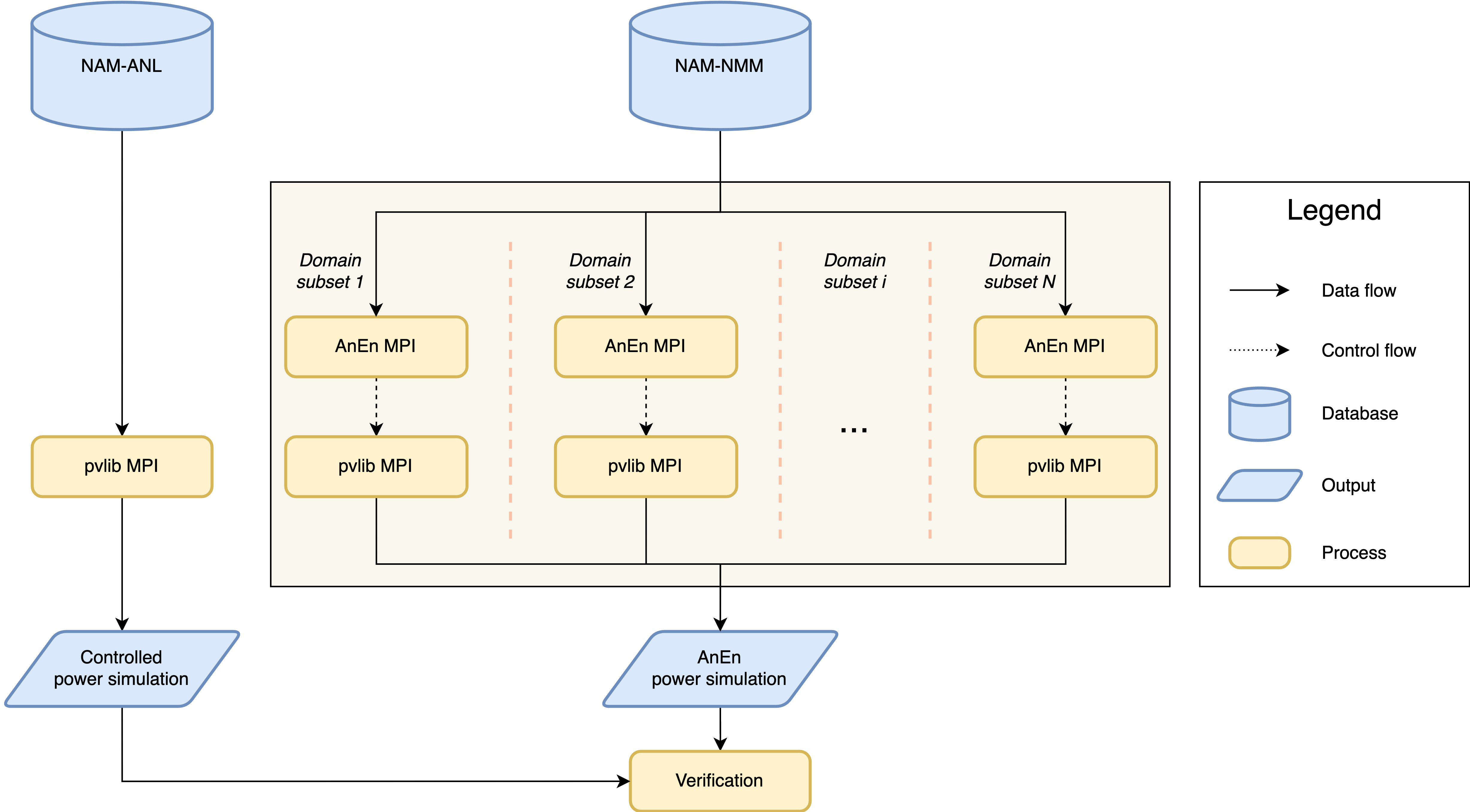
Figure 4: The schematic diagram for simulating PV power production with AnEn

Figure 4 shows the proposed framework for integrating the multivariate AnEn, as implemented by PAnEn [37], and the performance simulation system, as implemented with PV_LIB [38]. It consists of a controlled power simulation run initialized with NAM-ANL and a batch of experimental power simulation runs initialized with AnEn and NAM-NMM. This workflow is highly scalable because the generation of AnEn can be partitioned into geographic sub-domains and run concurrently. The computation for each sub-domain can be done independently, leading to a low overhead cost of communication. This parallelization is made possible thanks to the de facto standard of Message Passing Interface (MPI) for distributed computing and the workload manager, RADICAL EnTK, developed by the RADICAL Research Group at Rutgers University. An detailed discussion on the EnTK is provided in Section 5.

Table 2: Selected solar modules for simulation. Rows are sorted based on the STC rating decreasing

PV_LIB ID Code Area ($m^{2}$) Material # cells in series Year STC rating ($W$) Efficiency ($\%$) SunPower_128_Cell_Module__2009__E__ SP128 2.144 c-Si 128 2009 400 18.7 SunPower_SP305_GEN_C_Module__2008__E__ SP305 1.63 c-Si 96 2008 305 18.7 Silevo_Triex_U300_Black__2014_ STU300 1.68 c-Si 96 2014 300 17.8 Suniva_Titan_240__2009__E__ ST240 1.643 c-Si 60 2009 240 14.7 BP_Solar_BP3232G___2010_ BP3232G 1.6068 c-Si 120 2010 230 14.8 Sharp_ND_216U1F__2008__E__ ND216U1F 2.63 mc-Si 60 2008 215 8.3 Solar_Frontier_SF_160S__2013_ SF160S 1.22 CIS 172 2013 160 13.2 Kyocera_Solar_KD135GX_LP__2008__E__ KD135GX 1.002 mc-Si 36 2008 135 13.47 Kyocera_Solar_KC85T__2008__E__ KC85T .656 mc-Si 36 2008 85 13.4 First_Solar_FS_272___2009_ FS272 .72 CdTe 116 2009 72.5 10.07 Kyocera_Solar_KS20__2008__E__ KS20 .072 mc-Si 36 2008 20 28

Finally, the workflow is repeated for 11 different solar panel types. There are, in total, 523 built-in solar modules in PV_LIB (as of pvlib v0.8.1) provided by the Sandia Module database and 21,535 from the Clean Energy Council module database. Even with access to supercomputers and a large allocation, it is prohibitive to simulate all the modules. It is also unnecessary, because while all panels are different, they can be clustered into groups of similarly behaving panels.

Clusters were generated using the size of the solar panel, the total number of PV cells in a series, and the STC power rating for the panels in the Sandia Module database, and we carried out a clustering analysis to identify 11 module clusters. We then select the module with the maximum STC rating from each cluster. A summary of the selected solar modules is provided in Table 2.

4 Results and Discussions

Hourly day-ahead PV power production simulation for 2019 with a spatial resolution of 12 km has been carried out over CONUS. Because the power production at night is zero, only daylight hours were used. This leads to a different number of daily forecasts because for each location the length of the days varies throughout the year.

AnEn has 21 members and uses a two-year search period start at January 1, 2017, with the operational mode. Please recall that, in the operational mode, the search period is accumulated as the test time moves forward. Each of the 21 members is used to simulate power production. In the next section, results are shown for the weight optimization of the multivariate AnEn generation and the power simulation ensembles.

4.1 Weight Optimization for Multivariate Analog Ensemble Generation

One of the important input for AnEn is the set of predictor weights. Previous research employed a brute-force search that experiment different combinations of weights for each predictor, say from 0 to 1 with an increment of 0.1. This is, by nature, a computationally expensive task. Because all weights are normalized, a simple optimization is to force all weights to add up to 1.

In this study, the weight optimization follows this practice. However, having one set of weights (hereafter Equal Weighting (EW)) for the entire region of CONUS is not optimal because of the large domain coverage which calls for different optimal weights. On the other hand, optimizing for each of the 56,776 grid points is too computationally taxing. As a compromise, two alternative approaches are discussed to set weights for each of the grids.

1. The first approach optimizes weights from a sample of equally-spaced grids within CONUS and each grid is assigned the weights of the nearest sample point (hereafter Nearest Neighbor (NN)). The sample points have a latitudinal spacing of 4.5° and a longitudinal spacing of 3.5°.

2. The second approach uses a hierarchical clustering algorithm based on four features, including orography, annual GHI, temperature, and the average cloud cover. The rationale is that these four parameters inform the geographic and meteorological regimes (hereafter Regime Based (RB)).

For both methods CRPS is the metric or objective function being minimized, and it is computed at the center points of the NN sample grids, or for RB at a random sample of points from each cluster using data for 2018. The CRPS is calculated based on the actual power generation from the PV system rather than on the GHI, which is the real quantity of importance for this research. Rather than trying all 11 panels, the optimization is performed only on a single PV module, specifically the Silevo Triex U300. This was chosen due to its relatively large power capacity of 300 $W$ and its popularity in real world installations.

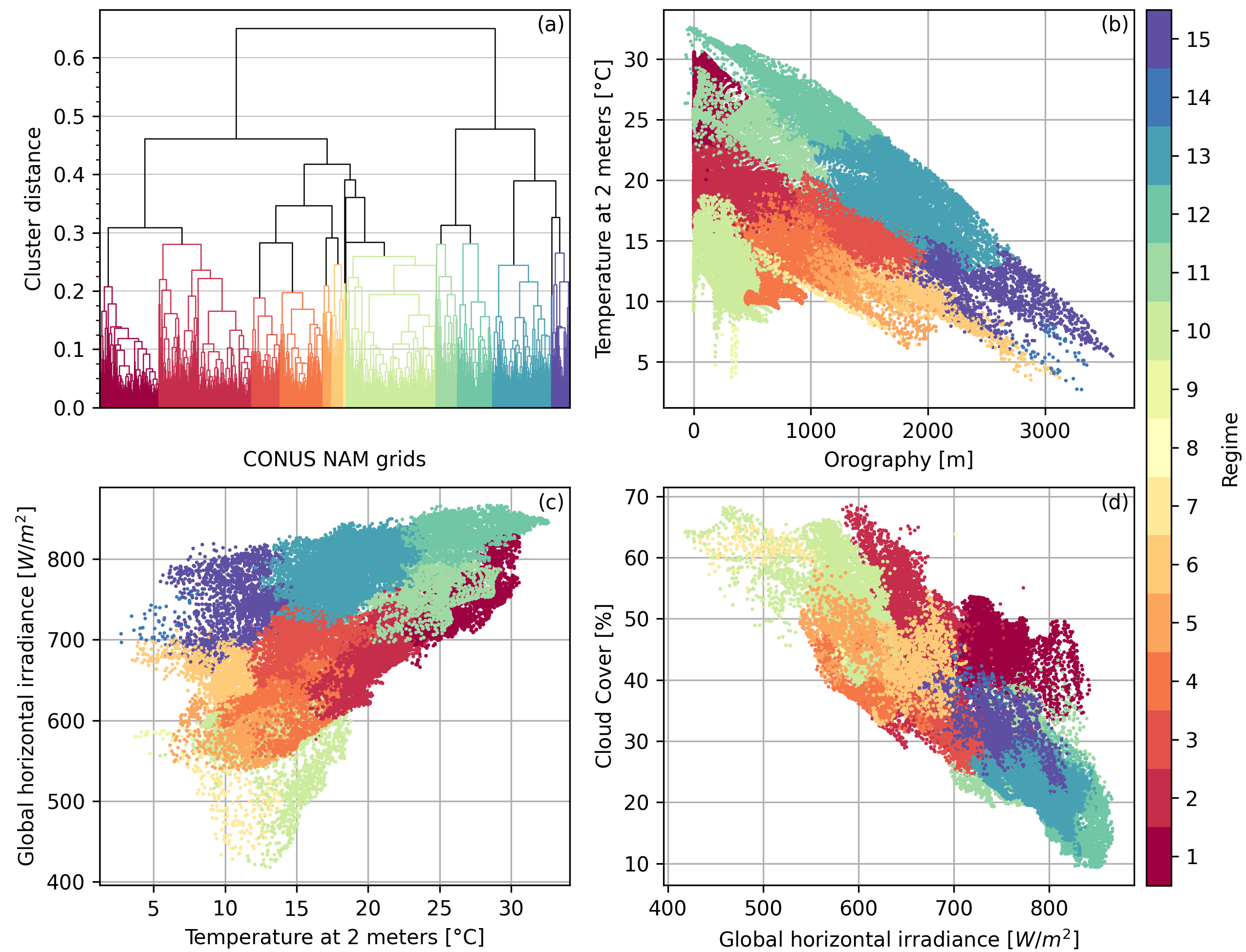
Figure 5: Hierarchical clustering of NAM-NMM grid points: a dendrogram representing the calculated hierarchical clusters (a) and scatter plots of predictors used to build the hierarchical clusters (b, c, d). Individual clusters are color coded.

Figure 5 shows how the clusters are defined. The hierarchical clustering algorithm is alternative to the well known K-Mean algorithm, and it differs in not requiring the number of clusters as input. Rather, the number of clusters is based on point distances.

There are two sub-categories of the hierarchical clustering, divisive and agglomerative [48, 49]. In agglomerative clustering, the algorithm starts by assigning each grid point to its own cluster, and then follows an iterative process where the two closest clusters are merged. Different metrics can be used to define the distance between clusters, e.g., using the shortest pair of points from two clusters or using the average distance between two clusters. The first definition is used when there are clear-cut shapes in the data; whereas the second definition is used when geographic locations are naturally correlated and variables tend to change smoothly [50]. Because of the high spatial correlation between grid points, this research uses the average distance between two clusters.

An effective way to visualize the process of the hierarchical clustering is through a dendrogram (Figure 5a). Clusters that are closer to each other are drawn closer along the horizontal axis. The clustering is an iterative process, meaning that, by the end of the process, there will only be one big cluster consisting of all the grid points. The height of a horizontal line connecting two clusters indicates the distance between merger clusters. This figure helps to decide the number of final clusters by providing information on how close the clusters are and how many points each cluster would have. We therefore, generated 15 clusters. Figures 5a, b, c show the relationship between variables used for clustering. The general correlation between variables is well-expected, e.g., a negative correlation between temperature and orography, or cloud cover and GHI; and a positive correlation between GHI and temperature. The clusters separate the regimes effectively, for example #15 corresponds to a regime of high elevation, low temperature, and high level of GHI.

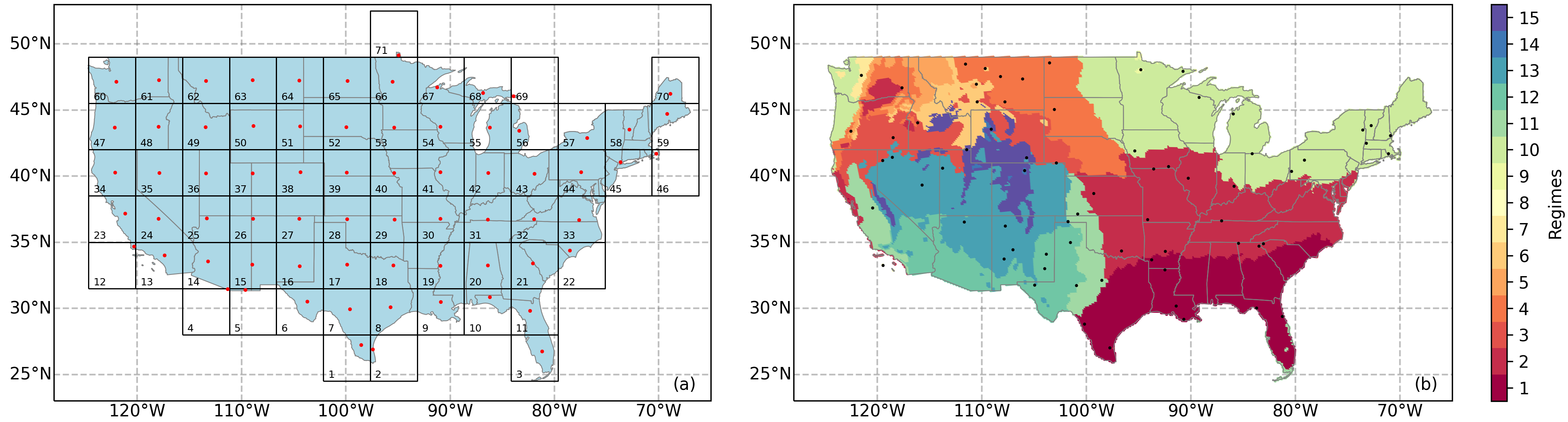
Figure 6: Geographic distribution of clusters determined from NN (a) and RB (b). There are 71 clusters and 15 clusters in NN and RB respectively. Samples points are shown in red (a) for NN and in black (b) for RB. NN clusters are labeled to the bottom left of each cluster. RB clusters are color coded. State boundaries are shown in grey lines.

Figure 6 arranges the NN and the RB clustering within the geographic context. Figure 6a shows the equally-spaced grid for each cluster. The red point shows the centroid location of the overlapped region for which weights will be optimized. Figure 6b shows the RB clusters and the black points show the sample locations where the weights are optimized. The total number of sample points from two approaches remains similar, with 71 for the NN and 70 for the RB. Figure 6b shows consistency with the IECC climate zones, shown in Figure 2. However, the determination of regimes is more dependent on solar-related features, while the climate zones are mostly defined by temperature and precipitation.

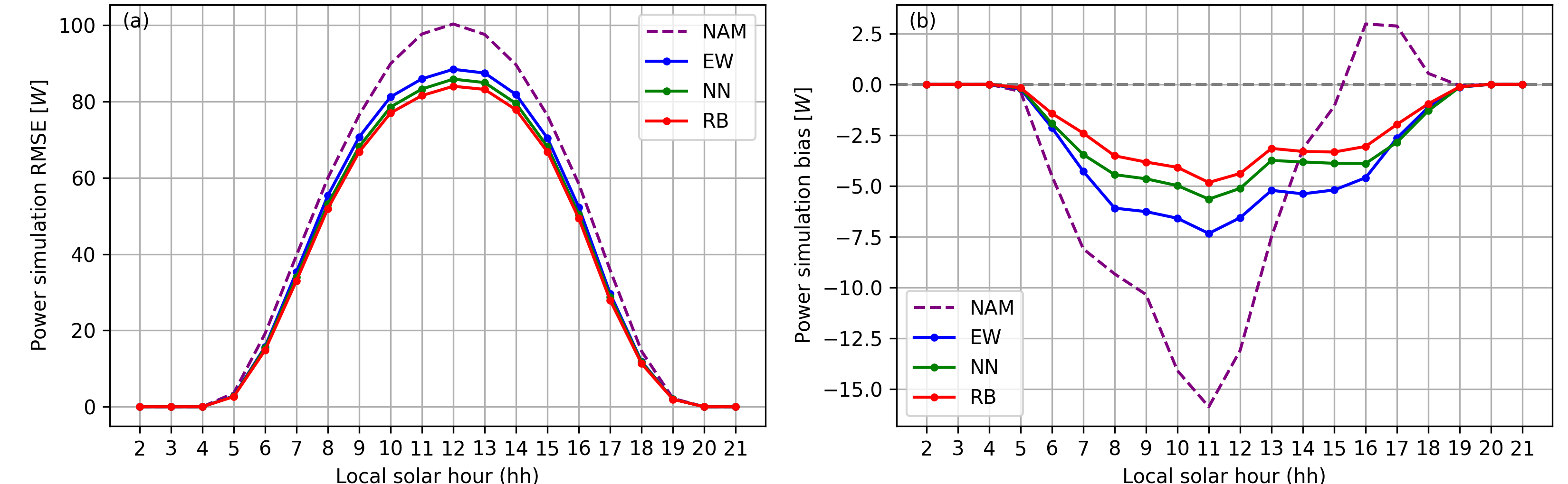
Figure 7: RMSE (a) and bias (b) of PV power simulation by forecast lead times for 2019 from four methods of comparisons: NAM, EW, NN, and RB. Forecast lead times from different geographic locations have been aligned with local solar time so that 12 is always the local solar noon.

A verification along space and time was used to evaluate the effectiveness of the optimized weights. Figure 7 shows the RMSE for four prediction methods, the baseline model NAM and three different AnEn results, each characterized by a different weighting strategies. The RMSE is calculated based on power simulation, meaning that both NAM and AnEn forecasts were used as input to the panel simulator. Model analysis has also been fed into the simulator to generate the most realistic version of what actually happened as the “ground-truth”.

NAM forecasts are computed in UTC times, which is not convenient when comparing large regions. Because CONUS effectively spans over four UTC time zones, significant artifacts are introduced when comparing far away regions like the East and West coasts. For example, generating forecasts for 17h00 UTC effectively means comparing forecasts for noon local time in New York with 09h00 local time in Los Angeles.

To avoid these inconsistencies, all computations are made in local time. However, rather than using the UTC time zone maps to carry out the time conversion, which adds an artificial transformation between solar time and a geographical region, the real solar noon is computed at each location, and the forecast lead times are realigned so that the forecast noon is the closest solar noon. Solar noon is the time when the Sun passes a location’s precise meridian and reaches its highest elevation in the sky. This time corresponds to the highest level of solar extraterrestrial irradiance, and on a clear sky day also corresponds to the highest level of surface irradiance. Because NAM provides hourly forecasts, the time difference between the solar noon and the forecast noon is at most $\pm$30 minutes.

Figure 7a shows the RMSE averaged across CONUS as a function of lead time for the AnEn ensemble means of EW, NN, and RB, and for the deterministic forecasts of NAM-NMM. On average, the RMSE of NAM-NMM peaks at solar noon with a value of 100 $W/m^{2}$. EW AnEn reduces the prediction error by 11.83%, from 100 to 88.42 $W/m^{2}$. However, using only equal weights for searching weather analogs is sub-optimal. AnEn NN and RB show results from the two optimizing schemes tested. NN reduces 14.41% of the prediction error of NAM-NMM from 100 to 85.85 $W/m^{2}$ and RB reduces it by 16.26% from 100 to 83.99 $W/m^{2}$. While the improvement is largest at solar noon, it follows the same trend for the other lead times, thus with RB, NN, EW and NAM consistently ordered from lowest to highest error (Figure 7a)

Figure 7b shows the prediction bias of the four methods. The bias is a verification metric that captures whether a weather model systematically over- or under-predicts. Ideally predictions should have a bias of zero, meaning that the forecasted ensemble mean always overlaps with the real mean. A positive bias, also referred to as a high bias, means that the forecasted ensemble mean is higher than the real mean. A negative bias, also referred to as low bias, is the opposite.

In terms of solar irradiance forecasts, NAM-NMM generally exhibits a negative bias during most of the day time but shifts to a positive value during afternoons. The peak value is a negative bias that occurs one hour before solar noon. Because the RMSE is increasing during this time while the bias improves slightly, an increase in random error is offsetting the bias improvement during this period of time.

All three modes of AnEn have better biases. At solar 11:00, when the bias of NAM-NMM is worst, the four methods have the bias of -15.87 $W/m^{2}$ (NAM), -7.34 $W/m^{2}$ (EW), -5.65 $W/m^{2}$ (NN), and -4.83 $W/m^{2}$ (RB).

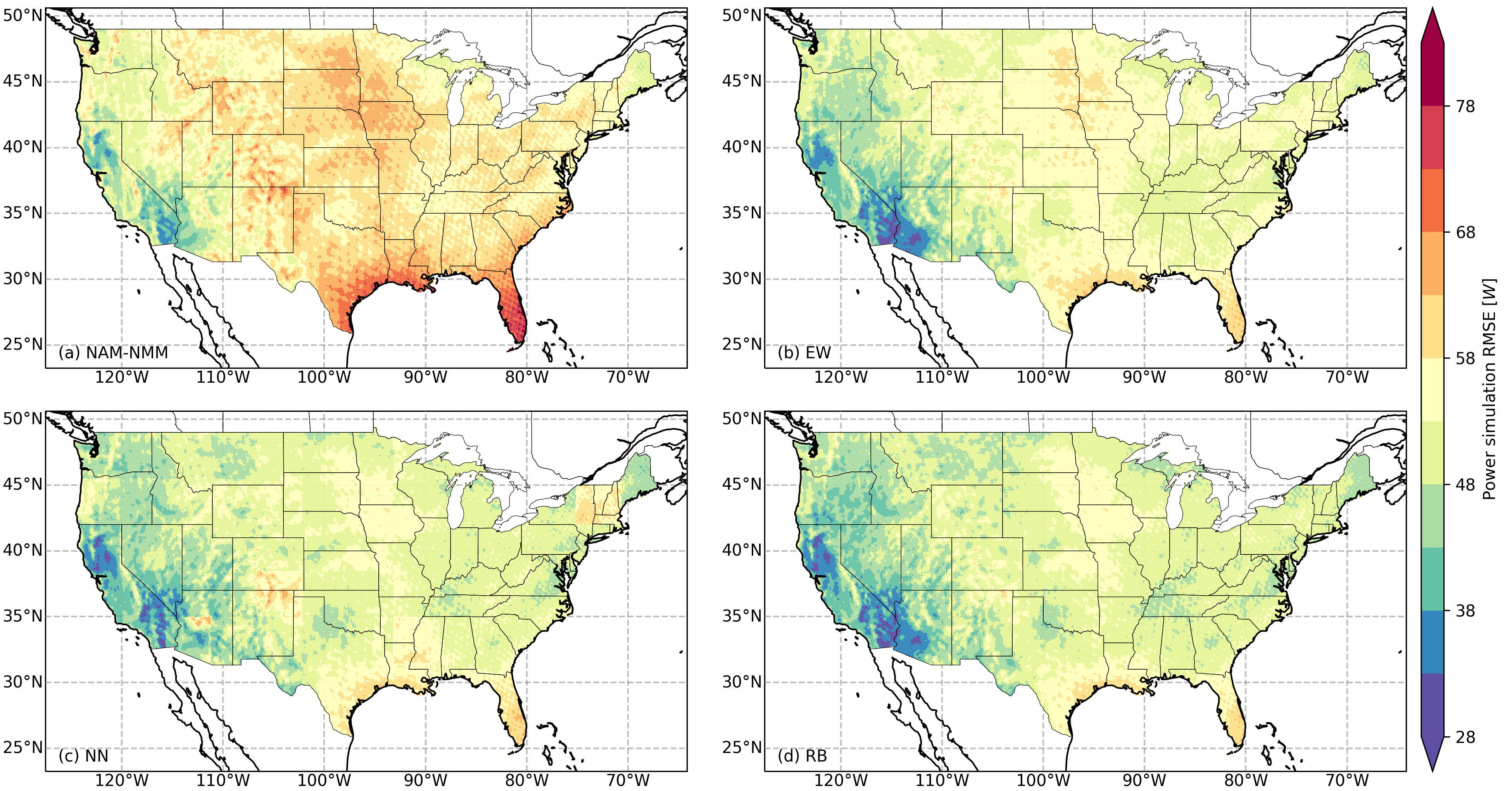
Figure 8: RMSE of PV power simulation averaged from all lead times for 2019 from four methods of comparisons: NAM (a), EW (b), NN (c), and RB. Coasts and state boundaries are shown in solid lines.

Figure 8 shows the RMSE maps of the entire domain for the four methods. Each pixel shows the yearly average of RMSE for all daylight lead times. Prominent in Figure 8a are two high error regions over Florida and Southern Texas. Figures 1c, d show that these two regions generally receive a high level of solar irradiance and total cloud cover. High levels of power production can be achieved because of the high solar irradiance, but the prediction error is also high due to high cloud cover.

However, another region is the Pacific Northwest which also has high cloud cover, instead, shows visibly lower prediction errors than that for Texas and Florida. This is mostly likely due to the different amount and variability of cloud cover. Clouds over the Pacific Northwest are regular and persistent, which is in part reflected by lower solar irradiance values (Figure 1c). The absolute error is therefore smaller because the magnitude of the power output is never as high as in Florida and Texas. Another feature to note in Figure 8a is the high accuracy over Arizona and the Southern California. These regions have high solar irradiance and low cloud cover, making them easier to predict.

Figures 8b, c, d show respectively the RMSE for EW, NN, and RB. All three methods show lower errors compared to NAM-NMM overall, as well as in specific areas. This can be attributed to the independent search of weather analogs with a fine spatial scale at each grid point. It allows the weather analogs to adapt to local weather regimes and correct the forecasts accordingly.

Figure 8 reveals one systematic problem with the NN approach. Recall from Figure 6a that, due to the computational limitations, it is unfeasible to run weight optimizations for each grid point. Only the center of grid points are used to compute the optimal weights, which are then reused for the entire grid of roughly 4.5°x3.5°. If a non-representative sample point for the entire grid is selected, incorrect weights are used for several points.

Its negative impact on prediction error is most noticeable for the 14th, 19th, 27th, and 58th regions in Figure 6. These regions have larger RMSE, surrounded by areas with noticeably lower errors. On the other hand, RB, that uses four variables (topography, solar irradiance, temperature, and cloud cover) to define various regimes, has a higher homogeneity in term of power production, which results in a smoother RMSE surface (Figure 8d).

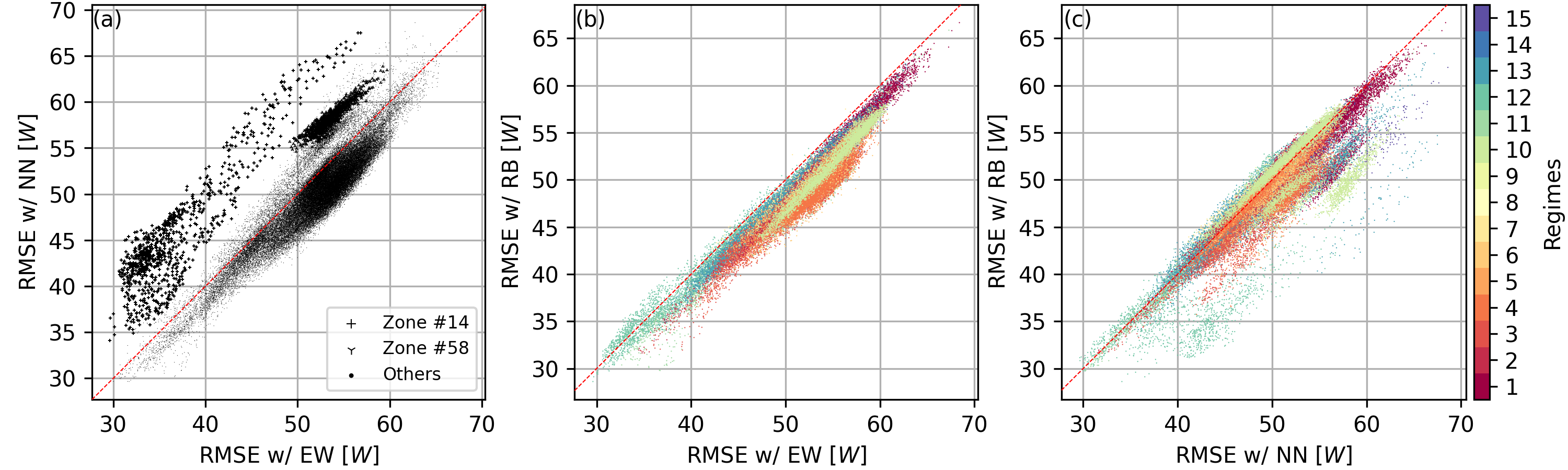
Figure 9: Scatter plots showing RMSE of PV power simulation for 2019: NN v.s. EW (a), RB v.s. EW, and RB v.s. NN. Each point in the scatter plots represents the verification statistic of a geographic location (a NAM grid point) calculated from all lead times during 2019. Two representative zones are highlighted with different point types in (a) with the index number corresponding to Figure 6a. Points are color coded based on regimes in (b, c) with a color mapping in consistent with Figure 6b.

Figure 9 shows scatter plots with pairwise comparisons for all modes of AnEn, along with a diagonal reference line. Points below the diagonal indicate that the method on the vertical axis is better. Figure 9a compares EW, on the horizontal axis, with NN, on the vertical axis. The majority of the points lie below the diagonal line, suggesting that NN outperforms EW. However, points from the 14th and the 58th (Figure 7a) grids are highlighted using different shapes, because they all show an inverse trend, indicating that the weight optimization failed for these regions.

These issues are likely to be solved by increasing the number of clusters, and reducing their geographical size. However, this will significantly increase computation time, which is what the method is trying to avoid. Without increasing the sample points, Figure 9b shows the comparison between the EW on the horizontal axis and the RB on the vertical axis. Please recall that the number of samples points are similar with 71 for the NN and 70 for the RB. The majority of points lie below the diagonal indicating the clear outperformance of RB compared to EW.

Figure 9c compares the NN and RB. The difference between these two methods are smaller than the previous comparisons because both methods (NN and RB) involve grid search but with differences in how regions are defined and samples are drawn. Yet, RB shows its outperformance over the NN for the regimes 10, 11, and 12 which overlaps with the NN clusters where non-representative sample points are chosen.

RB also demonstrates patterns of errors related to the spatial characteristics of the regimes. For example, the regime 1 covers the Southeastern CONUS associated with high solar irradiance and and middle-to-high cloud cover. Points are clustered, in Figure 9b, at the right tail of the spectrum, having a high error of power simulation. On the other side, regime 13 and 12 cluster at the left tail of the spectrum, having a low error of power simulation. These regimes are typically associated with middle-to-high solar irradiance but very low cloud cover. The clustering of error within RB regimes indicates the effectiveness of the regimes to separate different error patterns associated with NAM-NMM, and as a result, the predictor weights can be optimized focusing on correcting a particular type of error.

Table 3: Summary statistics calculated based on the hierarchical regimes define by the RB. Power simulation RMSE is calculated at local solar noon averaged across 2019 and from all grid points. * indicates that the RMSE of the RB is significantly different from that of NAM-NMM, the EW, and the NN at the level of $p=0.05$.

RB Regime RMSE at Solar Noon ($W$) GHI at Solar Noon ($W/m^{2}$) # Grids # Samples NAM EW NN RB 12 86.641 73.424 74.861 71.871 362.303 4225 5 3 91.641 82.355 80.444 76.961 301.824 3411 4 11 94.087 82.926 78.492 77.314 319.546 2615 3 13 92.382 82.056 81.237 79.817 342.535 7105 8 7 93.546 84.277 79.760 82.431 176.769 208 1 5 94.271 87.009 83.442 82.604 234.463 1045 2 4 100.165 89.482 85.378 83.068 273.874 5188 6 6 98.555 89.330 86.413 84.098 267.284 1477 2 2 101.926 90.213 86.498 85.399 272.640 11221 13 15 102.211 91.227 88.748 87.301 318.927 2160 3 10 101.705 93.053 89.207 87.607 239.381 10884 12 1 112.170 92.922 91.834 89.009 289.397 7134 8 9 110.560 96.758 90.027 92.894 258.179 33 1 14 110.357 95.756 94.004 94.017 290.165 68 1 8 143.911 117.995 118.537 116.924 227.277 2 1 Summary 102.275 89.919 87.259 *86.088 278.304 56776 70

Table 4: Summary statistics aggregated from IECC climate zones. Power simulation RMSE is calculated from different parts of the day and averaged across 2019 and all grid points: morning hours from 8 AM to 10 AM, noon hours from 11 AM to 1 PM, and afternoon hours from 2 PM to 4 PM. * indicates that the RMSE of the RB is significantly different from its counterpart of NAM-NMM, the EW, and the NN at the level of $p=0.05$.

IECC Climate Zone RMSE during Morning ($W$) RMSE during Noon ($W$) RMSE during Afternoon ($W$) # Grids NAM EW NN RB NAM EW NN RB NAM EW NN RB 1A 92.159 71.736 71.549 69.321 129.349 105.522 105.502 104.020 106.667 88.859 88.370 88.135 72 2A 90.326 77.156 76.485 74.920 115.530 96.823 95.377 93.812 87.083 76.633 75.332 74.272 3021 2B 72.862 60.536 66.694 60.457 88.260 71.653 77.103 70.901 65.935 55.248 60.235 54.357 1061 3A 78.575 71.876 70.402 68.229 100.953 88.554 86.707 83.941 79.173 71.294 69.726 67.754 6621 3B 71.429 62.419 60.788 60.062 88.596 76.456 74.795 73.735 67.588 60.503 58.947 57.821 4350 3C 68.007 58.530 56.144 55.821 80.987 73.096 70.623 70.044 62.498 54.722 52.545 51.704 395 4A 76.997 70.917 68.056 67.503 98.880 88.183 84.665 83.641 76.653 69.828 67.127 66.426 6049 4B 72.845 65.486 65.151 62.753 94.035 80.596 81.420 77.660 76.439 69.087 69.432 66.643 2150 4C 71.933 66.813 66.272 63.700 90.069 83.501 82.578 79.425 66.980 61.967 61.641 58.162 1139 5A 79.830 74.841 70.627 70.118 100.940 91.193 86.295 85.450 75.443 70.100 66.491 65.752 7068 5B 71.148 62.947 61.103 59.838 90.951 80.541 79.091 77.493 71.695 65.183 63.423 62.053 8931 6A 77.192 73.617 70.074 68.900 101.898 92.408 89.019 86.991 74.903 69.967 67.080 65.869 5870 6B 72.740 68.634 64.640 62.710 97.529 88.247 84.517 82.523 76.649 71.578 68.109 66.624 6518 7 71.947 70.265 65.768 65.368 100.260 90.829 86.651 85.569 75.322 70.253 67.159 66.396 3069 Summary 76.285 68.269 66.697 *64.978 98.445 86.257 84.596 *82.515 75.930 68.230 66.830 *65.141 56314

Finally, Table 3 and Table 4 compare the forecast error based on two different geographic clustering criteria. Table 3 averages errors from the regimes defined by the RB. Rows in the table are sorted based on the RMSE of the RB from the lowest to the highest. Verification results are shown for the solar noon only because that is genearlly when the solar irradiance and the power production reach the climax.

The RB mostly achieves lower errors compared to the NN except for the regimes 7, 9, and 14. RB only has one sample point for each of these regimes, making it subject to the same issue NN has. However, these regimes are tend to be small clusters and therefore have weaker impact to the overall predictability, unlike in the case of NN, each sample point will have an equal impact due to the same size of each cluster. On average, at the solar noon, the RB has the lowest prediction error. The average statistics is consistent with Figure 7a at solar noon time.

It is possible that RB outperforms the other methods simply because the verification is aggregated in favor of how RB is optimized. To rule out the potential bias, an independent clustering, from the IECC climate zones, is used to average errors, as shown in Table 4. The total number of grids within the IECC climate zones is smaller (462 points, 0.8%) than the total number of grid points within CONUS as defined by NAM-NMM, because of a slight difference in the coordinates mostly along the coasts (not shown).

Similar results can be observed that RB predominately remains the best method compared to NAM-NMM, the EW, and the NN. In general, error reduction during the noon is larger than the reduction during the morning and the afternoon. The climate zone, $3C$, is shown to have the lowest prediction error throughout the day and methods. It is, again, associated with high solar irradiance and low cloud cover.

It is therefore concluded that RB is a more reliable and effective weight optimization method for problems where a tradeoff must be found between computing weights for a large geographic region, and limited computational power available.

4.2 Predictability Assessment of Solar Panel Configuration

Section 4.1 evaluates two approaches to weight optimization for AnEn predictions. Results have been shown that RB is significantly better and more reliable for a large geographic domain. In this section, predictor weights optimized by the RB method is used to generate AnEn forecasts. Weather ensembles are then used with 11 PV modules (Table 2) to simulate power production.

PV systems are simulated with a 10 $KW$ capacity by the linear scaling of a particular type of panel in a series. For example, according to Table 2, the panel, SP128, has 400 $W$ capacity. Therefore, the simulated system contains 25 such panels in series to achieve the desired power of 10 $KW$. It is possible to connect PV modules in parallel to account for shading, but it requires extra wiring. Currently, connecting modules in series remains the most common practice because it generates maximum power output while at the same time being cheaper to install. In this PV system, we do not compensate for scaling and conversion losses, which depend on the type of inverter used.

Each PV system is run with hourly forecasts from AnEn for 2019. Since AnEn forecasts have 21 members, power simulation also has 21 members for each of the 11 systems.

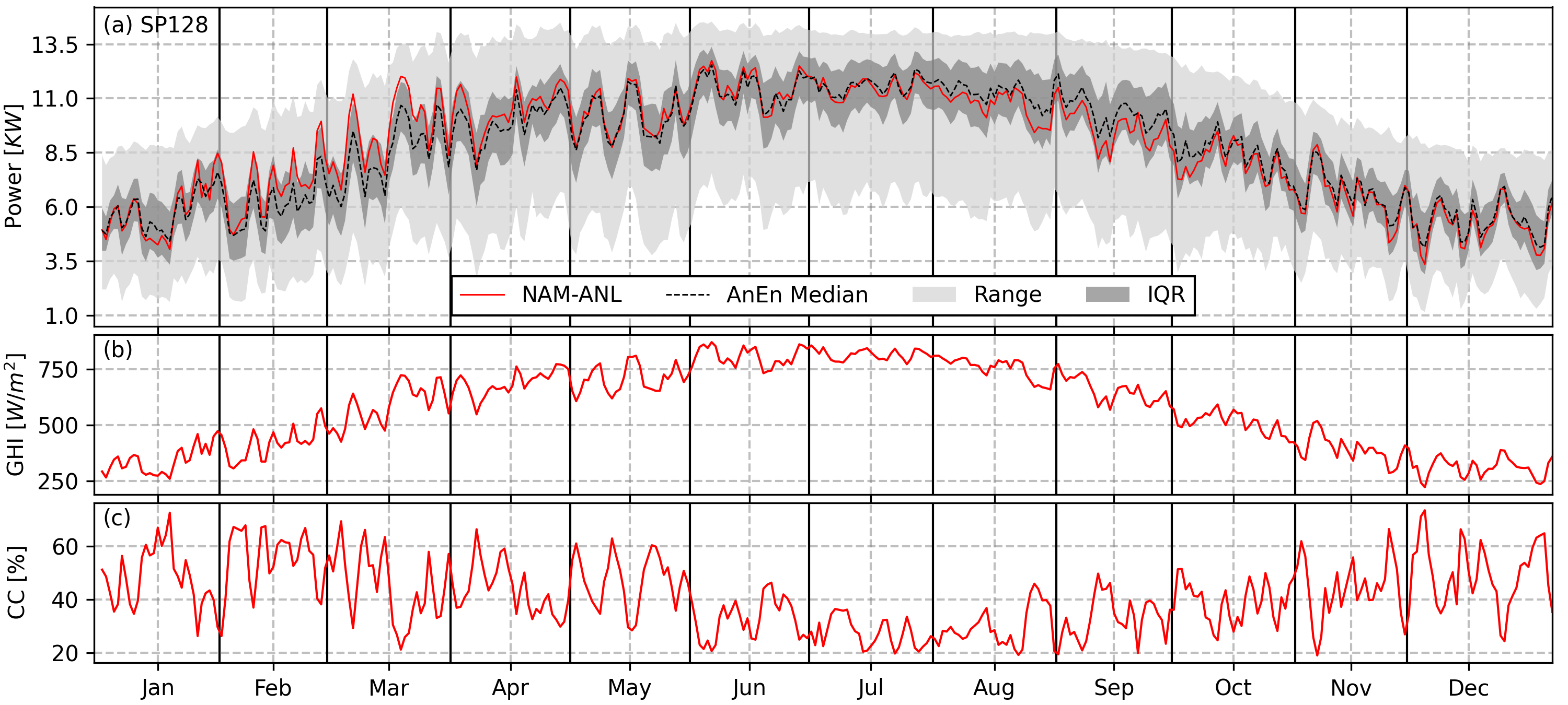
Figure 10: 21-member power simulation ensemble from the 10 $KW$ PV system with the module, $SP128$ for 2019. Only the power production at noon for each day is shown. NAM-NMM is shown in solid red; the ensemble median is shown in dashed black; the shaded colors indicate the ensemble range and the Inter-Quantile Range (IQR). (b, c) show the corresponding solar irradiance and cloud cover from NAM-NMM.

Figure 10 gives an example of the simulated power ensemble from SP128. The figure shows the power production at solar noon on each day in 2019. Values are averaged across all CONUS grid points. Figures 10a, b show a high positive correlation. However, the GHI reaches its climax during July while the power generation enters a production plateau starting around the early June. This is due to the saturation of the 10 $KW$ PV system.

The power ensemble range has a noticeable decrease going from May into June. This decrease correlates with the change of cloud cover at the same time. The predictability is, therefore, impacted by the cloud cover condition. The pattern can also be observed by compared the the model analysis (the red line) to the ensemble median (the black dashed line). In March when there is a significant amount of cloud cover, power simulation is less accurate, during which model analysis is barely covered by the 50% range of the simulation ensemble. In July, on the other hand, when there is a low level of cloud cover, power simulation is more accurate and the model analysis almost overlaps with the median of the simulation ensemble. This trend is consistent also for other months of the year.

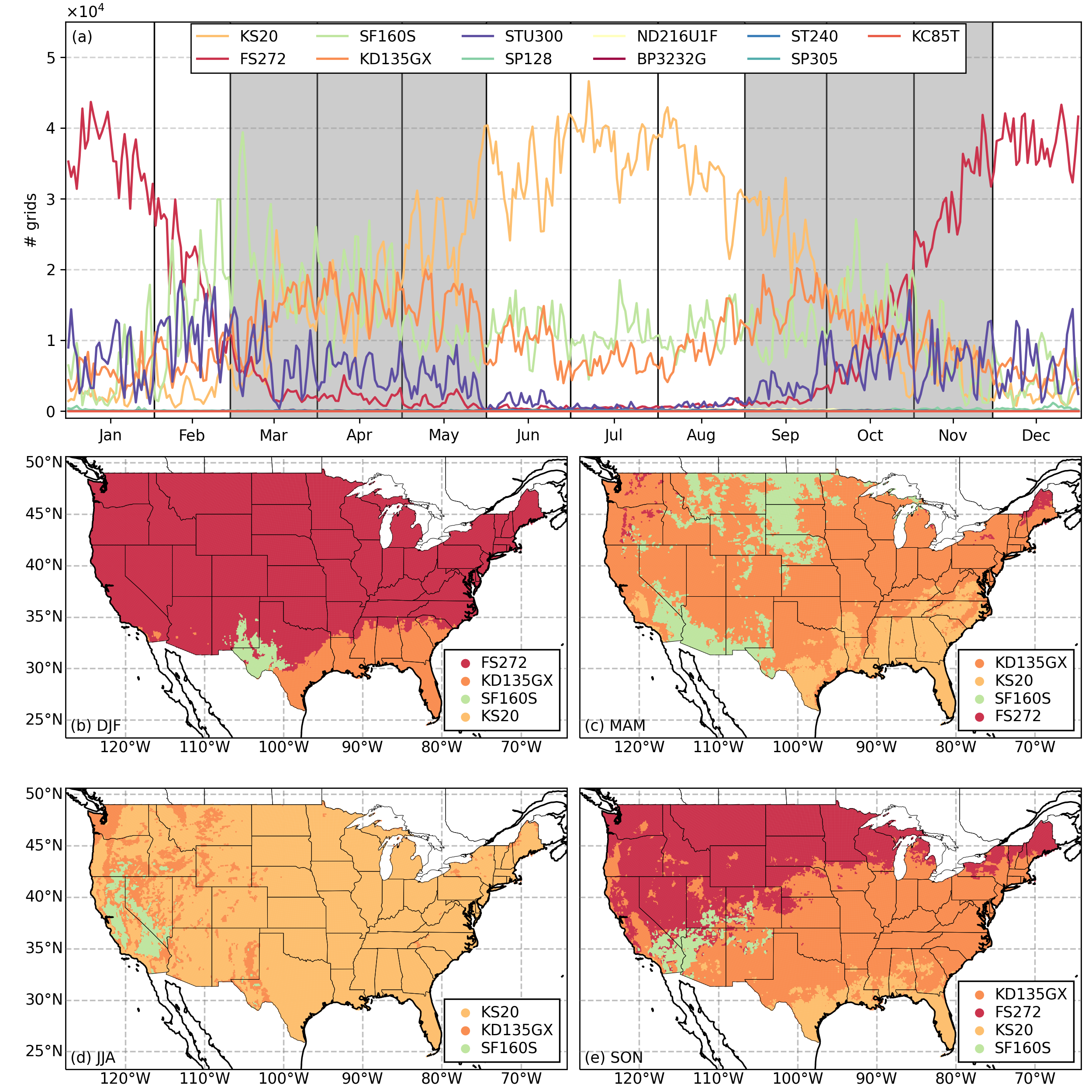
Figure 11: (a) shows the number of grid points against time where a particular PV module has the lowest simulation RMSE. (b, c, d, e) show the geographic map of CONUS color coded to the corresponding PV module with the seasonal lowest RMSE. The labels in the legend are sorted based on the average number of grids decreasing.

Figure 11 compares the year-round power simulation error from 11 PV systems both in space and time. Figure 11a shows the total number of grid points where a particular PV system outperforms all other modules in terms of daily RMSE averaged across CONUS; Figures 11b, c, d, e, show the geographic distribution of the outperforming panel based on seasonal RMSE.

In general, two types of modules stand out, KS20 and FS272. These two modules have the capacity of 20 $W$ (KS20) and 72.5 $W$ (FS272) respectively and they are among the smallest PV modules out of the 11 simulated modules. During the winter (Figure 11b), FS272 is preferred on more than 85% of the grid points. In the Northern CONUS, FS272 is the preferred panel, while the larger panel, KD135GX, with a capacity of 135 $W$, is preferred in the Southeastern CONUS. SF160S with a capacity of 160 $W$ is preferred in Western Texas and Southern New Mexico. Since there is significantly more cloud cover over Northern CONUS during the winter, results suggest that the power production of a PV system with smaller module capacity but a larger module quantity can be better predicted.

During the spring when solar irradiance starts to increase, larger panels starts to take dominance (Figure 11b). However, there might not be a clear winner because the total numbers of outperforming grids for the three panels, SF160S, KS20, and KD135GX, appear to be very similar (Figure 11a). The region that previously prefers FS272 shifts to KD135GX with the capacity almost doubled from 72.5 $W$ to 125 $W$. This suggests the predictability of power production is related not only to weather conditions, but also how a particular PV module responds to the changing weather conditions.

During the summer (Figures 11d), KS20 becomes the prevailing choice thanks to its relatively small size and small capacity, therefore easy to predict. Solar irradiance typically reaches year-round climax during the summer. An exceedingly high level of irradiance leads to PV modules generating more power than the nominal capacity but also with a higher-than-usual cell temperature. Under this weather condition, simulations have shown that smaller panels are more predictable in terms of power production. Opposite to this trend, the Pacific Northwest tends to have persistent cloud clover and relatively low solar irradiance even during the summer. Therefore, a larger panel, KD135GX, is preferred because the working environment is not as radiant.

Finally, the fall shows a geographic transition from north to south favoring, in turns, the modules FS272, KD135GX, and KS20. This is the time of the year when the solar irradiance remains relatively high while the cloud cover slowly increases. A smaller panel is preferred in the north due to high cloud cover and in the south due to over-performance.

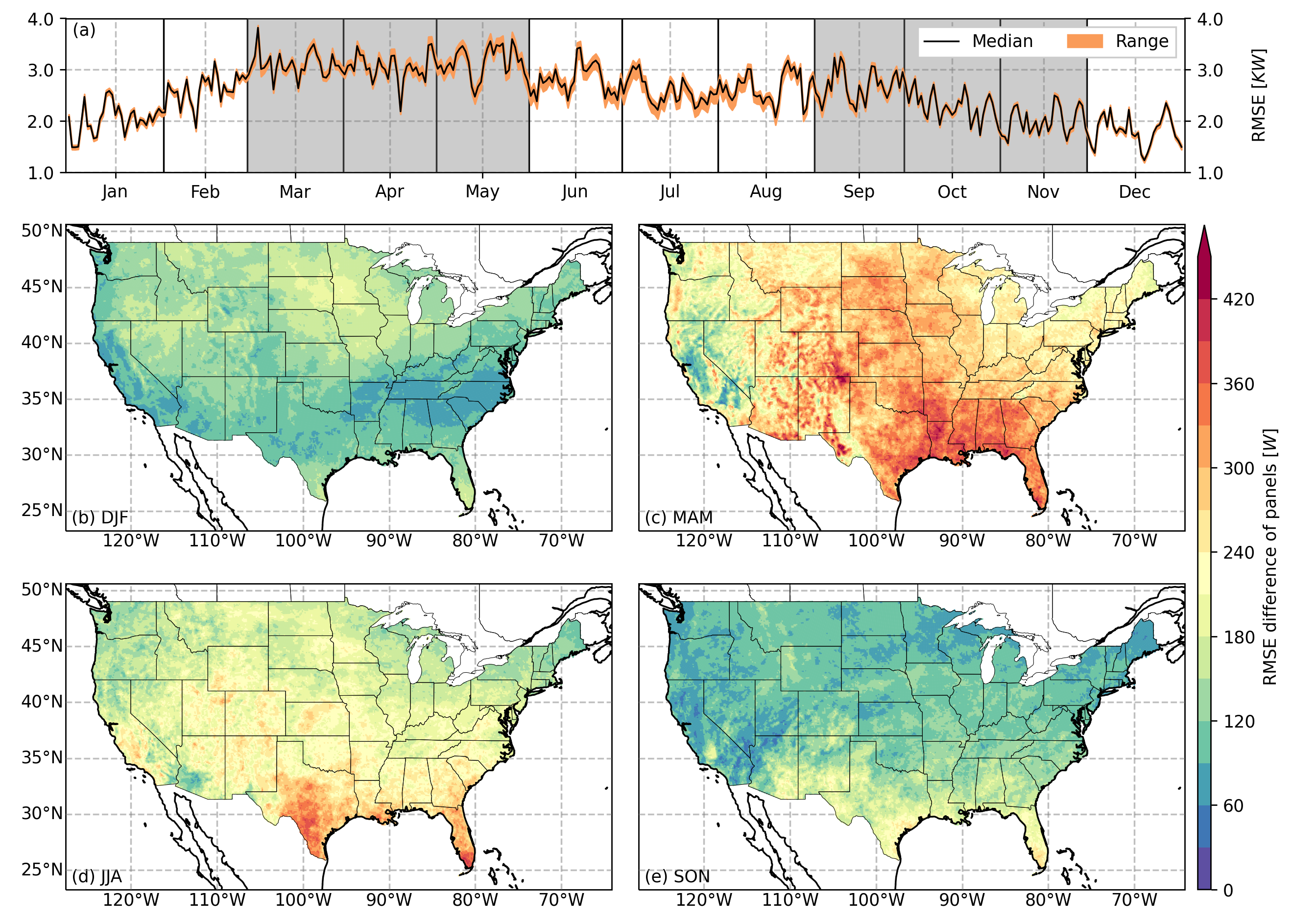
Figure 12: (a) shows the hourly power simulate error of the 10 $KW$ PV system with the 11 simulated modules. The spread shows the range of simulate error. (b, c, d, e) show the simulate error range aggregated by seasons.

Figure 11 compares the 11 PV systems by showing outperformance, but it falls short at showing how different the power production is from the systems. Figure 12 demonstrates how the simulation error differs among the 11 PV systems.

Figure 12a shows the median of the simulation error from the 11 PV systems in a black solid line and the range of simulation error in an orange shade. The simulation error is calculated for solar noon on each day in 2019 and then average within a particular ensemble. The range then shows the deviation of errors from 11 PV systems.

Figures 12b, c, d, e show the seasonal maps of the simulation error range. For a particular grid point, the seasonal RMSE from the worst performing module (already averaged over the 21 weather ensembles) is subtracted by the RMSE from the best performing module. This difference in error shows the potential improvement which can be expected when using the PV panel that is best at the location.

It is important to point out that the power simulation of a 10 $KW$ system has a very fine granularity, meaning that power prediction for each individual PV module is linearly scaled after being simulated. The prediction error is, therefore, higher than what was shown in previous literature [8, 51, 23, 52]. The reason why the linear scaling is required is because of the unavailability of dense observed power records over CONUS. Previous research, in fact, used observations from a limited sample of locations. An additional difference is that the current research does not focus on predicting the output of a power plant, but rather simulating the production for individual modules, which are then scaled to the power output desired.

The RMSE has an increasing trend in the winter and a decreasing trend in the fall (Figure 12a) which correlates well with the yearly pattern of solar irradiance. However, on average, the GHI is below 500 $W/m^{2}$ for these two seasons (Figure 10b) and PV panels are known not to produce high power during this period. Therefore, the predictability of the 11 PV systems is similar due to the relatively low power production, shown by the small range in Figure 12a and the mostly blue region in Figures 12b, e.

During spring and summer the predictability of power systems starts to differ. The RMSE, on average, drops from 3 $KW$ to 2.5 $KW$ from the spring going into the summer (Figure 12a), due to the decrease of cloud cover. But the range of the RMSE remains large compared to the fall and the winter. Persistent cloud cover and high level of solar irradiance in the spring are likely to affect the predictability of power production. A larger predictability difference appears in Southern and Midwestern U.S. (Figure 12c), reaching around 420 $W$ of RMSE difference, equivalent to 14% of the average RMSE and 4.2% of the total power generation.

During the summer, situations are slightly different because clod cover is typically low but solar irradiance is highest, reaching 870 $W/m^{2}$. Without the impact of cloud cover, the overall seasonal difference of predictability (Figure 12d) is lower compared to that of the spring. It is also shown that Southern Texas and Southern Florida have large differences in the predictability when comparing the results of the 11 PV systems, with a RMSE difference of over 300 $W$, equivalent to more than 12%.

The difference in the RMSE, or the range of the RMSE from various PV systems is not caused by the difference in weather conditions because all power simulations have been carried out using the same weather input generated by AnEn. Therefore, the weather conditions are held constant when comparing power production from the PV systems. The difference is, however, caused by how each module performs under different weather conditions. Modules have different efficiency level and are made of different materials, and therefore respond differently to weather changes. As a result, while improving weather forecasts definitely helps predicting power production, the additional uncertainty introduced by simulating the modules also needs to be studied. In fact, as discussed earlier, the characteristic of the modules can account for over 12% of the prediction error.

Table 5: A summary of the year-around power simulation of all 11 PV modules and a composite scenario where a combination of modules are used for different locations. The analysis and forecasted power generation is a summation of hourly simulation for the entire year averaged from all grid points. The RMSE is averaged from all grid points and then normalized by the corresponding analysis column to show the percentage. Rows are sorted based on the RMSE percentage decreasing. * indicates that the RMSE of the composite scenario is significantly different from all other scenarios where only one module is used at the level of $p=0.05$.

Panel Analysis ($MW$) Forecasted ($MW$) RMSE ($KW$) RMSE (%) KC85T 25.1 24.49 745.97 2.97 ND216U1F 24.88 24.27 738.85 2.97 KS20 24.57 23.98 730.41 2.97 KD135GX 24.45 23.86 722.59 2.95 ST240 25.3 24.69 743.65 2.94 STU300 24.83 24.24 728.84 2.94 BP3232G 25.5 24.9 739.08 2.90 SP128 25.18 24.59 728.09 2.89 SP305 25.45 24.86 731.27 2.87 SF160S 25.17 24.6 711.77 2.83 FS272 24.88 24.32 703.02 2.83 Composite 24.80 24.24 699.82 *2.82

Table 5 summaries the annual power generation and the simulation errors from the 11 simulated PV systems from CONUS. The power generation (the Analysis and the Forecasted columns) is calculated as the sum of the hourly power production for the entire year of 2019 and then averaged across CONUS grid points. The RMSE is the annual power production error averaged across CONUS and then it is normalized by the analysis field to show the percentage. If two panels have the same normalized RMSE, then they are sorted based on the RMSE.

The largest simulated module, SP128, has a power capacity of 400 $W$, and it is ranked #4 (bottom-up) out of the 11 modules. The smallest simulated module, KS20, has a power capacity of 20 $W$, and it is ranked #9 (bottom-up) out of the modules. Although a higher power production is usually associated with a larger prediction error at the hourly temporal scale, this relation can change when analyzed at a different temporal scale, e.g., annual. On a yearly basis, SP128 is forecasted to generate 24.59 $MW$ of power, 610 $KW$ larger than that of KS20, yet the RMSE of SP128 still remains lower than KS20.

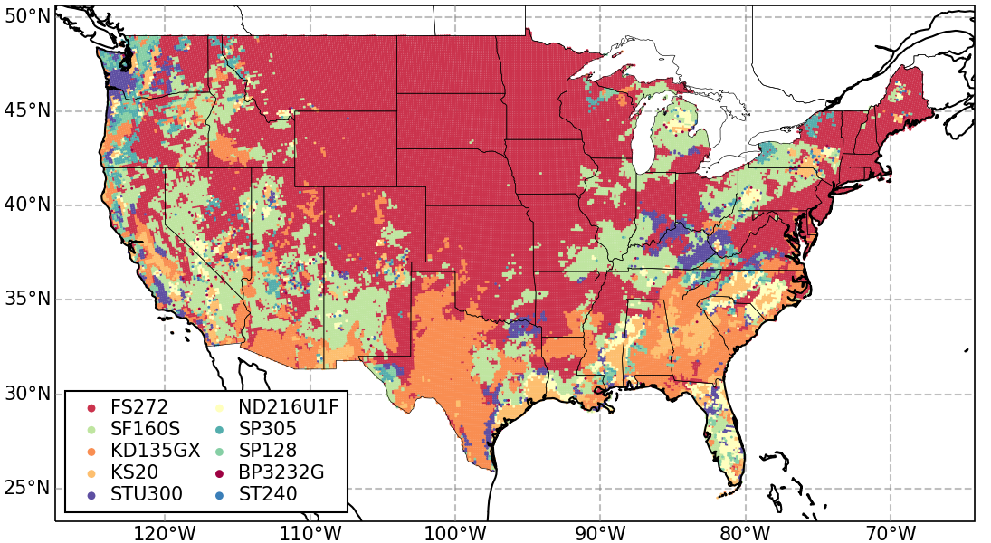
Figure 13: The map shows the geographic distribution of PV modules used in the composite scenario. The module with the lowest RMSE is used at each location to form the composite scenario. Coast and state boundaries are shown in solid lines. The labels in the legend are sorted column-wise based on decreasing the number grid points of a particular module.

The last row of Table 5 shows the results when using the best module at each location, rather than using the same panel for the entire CONUS. The selection of modules is based on optimizing the annual predictability and minimizing the prediction error. As a result (Figure 13), a majority of grid points prefer FS272 as the most predictable module, and this amounts to 31,108 grid points and 56.55% of all grid points. Following FS272 are SF160S (9,524 / 16.77%), KD135GX (7,436 / 13.10%), KS20 (2,445 / 4.31%), STU300 (1,728 / 3.04%), and ND216U1F (1,421 / 2.50%). These mentioned panels account for more than 95% of the grid points within CONUS and in total, there are 10 modules selected, leaving out KC85T. The exclusion of KC85T is also expected from Figure 11a that KC85T is ranked last (bottom-up) and there are few grid points throughout the year preferring this particular module.

With the 10-module portfolio for CONUS, the forecasted annual power generation is 24.80 $MW$ per grid and the RMSE is 699.82 $KW$. The prediction error achieves the lowest in comparison with other single-module scenario. Figure 13 shows the geographic distribution of the 10 modules in the composite scenario. FS272 is selected as the optimal module across the large area in the center-to-north of CONUS. This region features a low-to-middle level solar irradiance and a middle level of total cloud cover. Since the power production is not particularly high compared to other regions of CONUS, a smaller solar panel is preferred with 72.5 $W$ capacity. While an even smaller module, KS20, is available, it is not chosen due to the difference in predictability. The sub-region that covers Texas and the most part of Southeast features a exceedingly high level of solar irradiance and a fair amount of cloud cover. Modules tend to perform at a higher rate than the STC during summer. Under this condition, KD135GX with a 135 $W$ capacity is selected for the most regions. In Florida, where a even higher level of solar irradiance is found, it is impossible to identify a single panel which consistently outperforms the others. The final pattern shown in Figure 13 is the scattered regions favoring SF160S which occur across different and far-away geographical areas. These regions are characterized by either low cloud cover or relatively high solar irradiance.

5 Enabling Scalable Simulation via the RADICAL Ensemble Toolkit

RADICAL EnTK is a workflow engine a component of the RADICAL Cybertool (RCT) [53]. Those tools are software systems designed and implemented in accordance with the building blocks approach. Each system is independently designed with well-defined entities, functionalities, states, events and errors. Individual cybertools are designed to be consistent with a four-layered view of distributed systems for the execution of scientific workloads and workflows on High-Performance Computing (HPC) resources. Each layer has a well-defined functionality and an associated “entity”. The entities are workflows (or applications) at the top layer and resource specific jobs at the bottom layer, with workloads and tasks as intervening transitional entities in the middle layers.

RCT has three main components: RADICAL-SAGA (RS) [54], RADICAL-Pilot (RP) [55, 56] and RADICAL EnTK [57, 40]. RS is a Python implementation of the Open Grid Forum SAGA standard GFD.90 [58], a high-level interface to distributed infrastructure components like job schedulers, file transfer and resource provisioning services. RS enables interoperability across heterogeneous distributed infrastructures, improving on their usability and enhancing the sustainability of services and tools. RP is a Python implementation of the pilot paradigm and architectural pattern [59]. Pilot systems enable users to submit pilot jobs to computing infrastructures and then use the resources acquired by the pilot to execute one or more tasks. These tasks are directly scheduled via the pilot, without having to queue in the infrastructure’s batch system.

EnTK is a Python implementation of a workflow engine, specialized in supporting the programming and execution of applications with ensembles of tasks. EnTK executes tasks concurrently or sequentially, depending on their arbitrary priority relation. Tasks are scalar, MPI, OpenMP, multi-process, and multi-threaded programs that run as self-contained executables. Tasks are not functions, methods, threads or subprocesses.

5.1 Application Model

EnTK supports Ensemble-Based Application (EBA), where an ensemble is defined as a set of tasks. Ensembles may vary in the number of tasks, types of task, tasks’ executable (or executing kernel), and tasks’ resource requirements. EBA may vary in the number of ensembles or the runtime dependencies among ensembles. The space of EBA is vast, and thus there is a need for simple and uniform abstractions while avoiding single- point solutions.

Currently, the use cases motivating EnTK require a maximum of $O(10^{4})$ tasks but EnTK is designed to support up to $O(10^{6})$ tasks due to the rate at which this requirement has been increasing, especially in biomolecular simulations where a greater number of tasks is associated with greater sampling or more precise free energy calculations. EnTK supports resubmission of failed tasks, without application checkpointing, and restarting of failed RTS and components. In this way, applications can be executed on multiple attempts, without restarting completed tasks.

EnTK models EBA by combining the following user-facing constructs:

• Task: an abstraction of a computational task that contains information regarding an executable, its software environment and its data dependences.

• Stage: a set of tasks without mutual dependences and that can be executed concurrently.

• Pipeline: a list of stages where any stage $i$ can be executed only after stage $i-1$ has been executed.

The application consists of a set of pipelines, where each pipeline is a list of stages, and each stage is a set of tasks. All the pipelines can execute concurrently, all the stages of each pipeline can execute sequentially, and all the tasks of each stage can execute concurrently. Pipelines, stages, and tasks (PST) descriptions can be extended to account for dependencies among groups of pipelines in terms of lists of sets of pipelines. Further, the specification of branches in the execution flow of applications does not require to alter the PST semantics: Branching events can be specified as tasks where a decision is made about the runtime flow. For example, a task could be used to decide to skip some elements of a stage, based on some partial results of the ongoing computation.

5.2 Architecture

EnTK sits between the user and the HPC, abstracting resource management and execution management from the user. Figure 14 shows the components (purple) and subcomponents (green) of EnTK, organized in three layers: API, Workflow Management, and Workload Management.

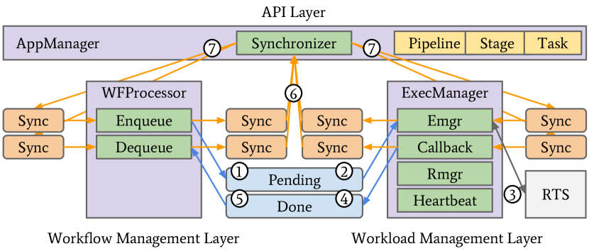
Figure 14: EnTK architecture and execution model. Components’ (purple) subcomponents (green) use queues (blue and orange) to communicate and coordinate the execution of an application via a chosen RTS (gray).

The API layer enables users to codify PST descriptions. The Workflow Management layer retrieves information from the user about available infrastructures, initializes EnTK, and holds the global state of the application during execution. The Workload Management layer acquires resources via the RTS. The Workflow Management layer has two components: AppManager and WFProcessor. AppManager uses the Synchronizer subcomponent to update the state of the application at runtime. WFProcessor uses the Enqueue and Dequeue subcomponents to queue and dequeue tasks from the Workload Management layer. The Workload Management layer uses ExecManager and its Rmgr, Emgr, RTS Callback, and Heartbeat subcomponents to acquire resources from infrastructures and execute the application. Another benefit of this architecture is the isolation of the RTS into a stand-alone subsystem. This enables composability of EnTK with diverse RTS and, depending on capabilities, multiple types of infrastructures. Further, EnTK assumes the RTS to be a black box enabling fault-tolerance. When the RTS fails or becomes unresponsive, EnTK can tear it down and bring it back, loosing only those tasks that were in execution at the time of the RTS failure.

5.3 Execution Model

EnTK components and subcomponents communicate and coordinate for the execution of tasks. Users describe an application via the API, instantiate the AppManager component with information about the available infrastructures and then pass the application description to AppManager for execution. AppManager holds these descriptions and, upon initialization, creates all the queues, spawns the Synchronizer, and instantiates the WFProcessor and ExecManager. WFProcessor and ExecManager instantiate their own subcomponents.

Once EnTK is fully initialized, WFProcessor initiates the execution by creating a local copy of the application description from AppManager and tagging tasks for execution. Enqueue pushes these tasks to the Pending queue (\raisebox{-0.96pt}1⃝ in Figure 14). Emgr pulls tasks from the Pending queue (\raisebox{-0.96pt}2⃝ in Figure 14) and executes them using a RTS (\raisebox{-0.96pt}3⃝ in Figure 14). RTS Callback pushes tasks that have completed execution to the Done queue (\raisebox{-0.96pt}4⃝ in Figure 14). Dequeue pulls completed tasks (\raisebox{-0.96pt}5⃝ in Figure 14) and tags them as done, failed or canceled, depending on the return code from the RTS.

Throughout the execution of the application, tasks, stages and pipelines undergo multiple state transitions in both WFProcessor and ExecManager. Each component and subcomponent synchronizes these transitions with AppManager by pushing messages through dedicated queues (\raisebox{-0.96pt}6⃝ in Figure 14).AppManager pulls these messages and updates the application states. AppManager then acknowledges the updates via dedicated queues (\raisebox{-0.96pt}7⃝ in Figure 14). This messaging mechanism ensures that AppManager is always up-to-date with any state change, making it the only stateful component of EnTK.

5.4 Integration of Parallel Analog Ensemble

The integration of the PAnEn and the RADICAL EnTK provides good examples for the ensemble-of-pipelines model and the pipeline-of-ensembles model.

The ensemble-of-pipelines model refers to the workflow where each pipeline is an independent execution unit that might consist of several stages and there are several such pipelines to execute in parallel. This type of model is adopted for weight optimization shown in Section 4.1. In total, there are 8,001 different weight combinations to experiment and each trial is independent from each other, meaning that the execution with one weight combination does not need to wait for or communicate with any other executions. Each trial consists of a pipeline following the process of generating weather analogs, simulation power production, and finally verifying power simulation results with the forecast analysis. The three stages should be executed in series and therefore, they have been placed with order in a pipeline. Since the processes need to be repeated for the NN and the RB, the final individual pipeline has six tasks in total.

The pipeline-of-ensembles model refers to the workflow where there are multiple sequential stages and each stage consists of tasks that will be executed in parallel. The later simulation of the 11 PV modules adopted this model by two stages:

1. Stage one: AnEn forecasts have been generated for each of the subset domain in parallel.

2. Stage two: Each of the 11 modules is used to simulate power production for the corresponding subset domain.

Note that since the computation for each subset domain is considered as an individual task, tasks can be executed in parallel. There are 71 subset domains for the NN and 28 for the RB. On the other hand, stages are executed in sequence because the power simulation can only be carried out after the AnEn forecasts have been successfully generated. EnTK offers a flexible interface for defining the computational requirement for each task so that each task can dynamically request a proper amount of allocation based on the area of the subset domain. Given that there are dozens of subsets with different area, this functionality frees the developer from having to specify the computation manually.

Table 6: Summary of experiment runtime and allocation request on NCAR Cheyenne

Experiment Size of workflow # cores Runtime (h) AnEn weight optimization 8,001 pipelines x 6 tasks per pipeline 7,200 1.31 Ensemble power simulation 2 stages x 99 tasks per stage 5,508 4.28

In general, the pipeline-of-ensembles model offers more efficient concurrency because it utilizes lightweight tasks. As a result, it is recommended to adopt this type of model as much as possible. The ensemble-of-pipelines model merely provides another layer of abstraction for users to create more complex scientific workflows. Table 6 summarizes the runtime and computational requirement of the two experiments executed on NCAR Cheyenne.

6 Final Remarks

Forecast ensembles typically offer higher prediction accuracy than deterministic predictions, and they provide additional information on uncertainty. However, running a ensemble NWP model usually involves both technical and computational challenges. Researchers often download forecast ensembles from archives, but the amount of accessed data can easily exceed dozens of gigabyte, sometimes terabyte. Designing a scientific workflow that involves simulation ensembles require parallelization and scalable tools.

This chapter demonstrates the ability of using the AnEn method and the RADICAL EnTK tools to design ensemble workflows at scale. First, deterministic predictions over CONUS for 2019 has been transformed into 21-member forecast ensembles using AnEn. The forecasts have a spatial resolution of 12 km and a temporal resolution of one hour. Second, the weather forecast ensembles are used to simulate point-by-point power production with 11 different PV modules. Over 110 TB of simulation data have been generated on the NCAR supercomputer, Cheyenne.

Results have shown that the predictability of solar power generation depends on not only the meteorological variation, but also the configuration of PV modules. In order to optimize the amount of predictable solar power, the type of PV modules should be an important factor to consider in its relation to geographic locations and its interplay with long-term weather conditions.

Appendix A A Minimal Workflow for Power Simulation

⬇

1import pandas as pd

2from pvlib import pvsystem, irradiance, location, atmosphere, temperature

3

4def simulate_power_production(

5 timestamp, latitude, longitude, ghi, alb, tamb, wspd,

6 tc_module, pv_module):

7 """

8 The core function for simulating power production under a given forecasted

9 weather condition and a solar panel configuration at a particular location.

10

11 This function is developed and tested with pvlib v0.8.1.

12 """

13

14 # Initialize a location

15 loc = location.Location(latitude=latitude, longitude=longitude)

16

17 # Calculate the solar position

18 solar_position = loc.get_solarposition(timestamp)

19

20 # Calculate extraterrestrial irradiance

21 dni_extra = irradiance.get_extra_radiation(timestamp)

22

23 # Calculate air mass

24 air_mass = atmosphere.get_relative_airmass(solar_position[’apparent_zenith’])

25

26 # Decompose DNI from GHI

27 dni_dict = irradiance.disc(ghi, solar_position[’zenith’], timestamp)

28

29 # Calculate sky diffuse

30 sky_diffuse = irradiance.haydavies(

31 0, 180, ghi, dni_dict[’dni’], dni_extra,

32 solar_position[’apparent_zenith’], solar_position[’azimuth’])

33

34 # Calculate ground diffuse

35 ground_diffuse = irradiance.get_ground_diffuse(0, ghi, alb)

36

37 # Calculate angle of incidence

38 aoi = irradiance.aoi(0, 180, solar_position[’apparent_zenith’],

39 solar_position[’azimuth’])

40

41 # Calculate in-plane irradiance components

42 poa = irradiance.poa_components(

43 aoi, dni_dict[’dni’], sky_diffuse, ground_diffuse)

44

45 # Calculate cell temperature

46 tcell = pvsystem.temperature.sapm_cell(

47 poa[’poa_global’], tamb, wspd, **tc_module)

48

49 # Calculate effective irradiance

50 effective_irradiance = pvsystem.sapm_effective_irradiance(

51 poa[’poa_direct’], poa[’poa_diffuse’], air_mass, aoi, pv_module)

52

53 # Calculate power

54 sapm_out = pvsystem.sapm(effective_irradiance, tcell, pv_module)

55

56 return sapm_out

57

58# Example usage

59pv_module = pvsystem.retrieve_sam(’SandiaMod’)[’Silevo_Triex_U300_Black__2014_’]

60tc_module = temperature.TEMPERATURE_MODEL_PARAMETERS[

61 ’sapm’][’open_rack_glass_polymer’]

62timestamp = pd.to_datetime(’2021-01-01 12:00:00’)

63

64simulate_power_production(timestamp, -77.86, 40.79, 400, 0.8, 27, 1.2,

65 tc_module, pv_module)

Listing 1: An example of PV power simulation with PV_LIB in Python

References

- Lewis and Nocera [2006] Nathan S Lewis and Daniel G Nocera. Powering the planet: Chemical challenges in solar energy utilization. Proceedings of the National Academy of Sciences, 103(43):15729–15735, 2006.
- Administration [2021] U.S. Energy Information Administration. Monthly energy review. Technical report, U.S. Energy Information Administration (EIA), 2021.
- Administration [2010] U.S. Energy Information Administration. Annual energy outlook 2020. Department of Energy, 92010(9):1–15, 2010.
- Dubin [2021] Kenneth Dubin. Eia projects renewables share of u.s. electricity generation mix will double by 2050, Feb 2021. URL https://www.eia.gov/todayinenergy/detail.php?id=46676.
- Ferruzzi et al. [2016] Gabriella Ferruzzi, Guido Cervone, Luca Delle Monache, Giorgio Graditi, and Francesca Jacobone. Optimal bidding in a day-ahead energy market for micro grid under uncertainty in renewable energy production. Energy, 106:194–202, 2016.
- Wen and David [2001] FS Wen and AK David. Strategic bidding for electricity supply in a day-ahead energy market. Electric Power Systems Research, 59(3):197–206, 2001.
- Davatgaran et al. [2018] Vahid Davatgaran, Mohsen Saniei, and Seyed Saeidollah Mortazavi. Optimal bidding strategy for an energy hub in energy market. Energy, 148:482–493, 2018.
- Alessandrini et al. [2015] S. Alessandrini, L. Delle Monache, S. Sperati, and G. Cervone. An analog ensemble for short-term probabilistic solar power forecast. Applied Energy, 157:95–110, November 2015. ISSN 0306-2619. doi: 10.1016/j.apenergy.2015.08.011. URL http://www.sciencedirect.com/science/article/pii/S0306261915009368.
- Chow et al. [2015] Chi Wai Chow, Serge Belongie, and Jan Kleissl. Cloud motion and stability estimation for intra-hour solar forecasting. Solar Energy, 115:645–655, 2015.
- Kleissl et al. [2013] Jan Kleissl, Juan Luis Bosch, Benjamin Kurtz, Matthew Lave, Israel Lopez, Patrick Mathiesen, Andu Nguyen, and Bryan Urquhart. Recent advances in solar variability modeling and solar forecasting at uc san diego. In Proceedings, American Solar Energy Society, 2013 Solar Conference, 2013.
- Wan et al. [2015] C. Wan, J. Zhao, Y. Song, Z. Xu, J. Lin, and Z. Hu. Photovoltaic and solar power forecasting for smart grid energy management. CSEE Journal of Power and Energy Systems, 1(4):38–46, December 2015. ISSN 2096-0042. doi: 10.17775/CSEEJPES.2015.00046. Conference Name: CSEE Journal of Power and Energy Systems.
- Jimenez et al. [2016] Pedro A. Jimenez, Joshua P. Hacker, Jimy Dudhia, Sue Ellen Haupt, Jose A. Ruiz-Arias, Chris A. Gueymard, Gregory Thompson, Trude Eidhammer, and Aijun Deng. WRF-Solar: Description and Clear-Sky Assessment of an Augmented NWP Model for Solar Power Prediction. Bulletin of the American Meteorological Society, 97(7):1249–1264, July 2016. ISSN 0003-0007, 1520-0477. doi: 10.1175/BAMS-D-14-00279.1. URL https://journals.ametsoc.org/view/journals/bams/97/7/bams-d-14-00279.1.xml. Publisher: American Meteorological Society Section: Bulletin of the American Meteorological Society.
- Dirnberger et al. [2015] Daniela Dirnberger, Gina Blackburn, Björn Müller, and Christian Reise. On the impact of solar spectral irradiance on the yield of different PV technologies. Solar Energy Materials and Solar Cells, 132:431–442, January 2015. ISSN 0927-0248. doi: 10.1016/j.solmat.2014.09.034. URL https://www.sciencedirect.com/science/article/pii/S0927024814005169.
- Huld and Amillo [2015] Thomas Huld and Ana M. Gracia Amillo. Estimating PV Module Performance over Large Geographical Regions: The Role of Irradiance, Air Temperature, Wind Speed and Solar Spectrum. Energies, 8(6):5159–5181, June 2015. doi: 10.3390/en8065159. URL https://www.mdpi.com/1996-1073/8/6/5159. Number: 6 Publisher: Multidisciplinary Digital Publishing Institute.
- Mills and Wiser [2011] A. D. Mills and R. H. Wiser. Implications of geographic diversity for short-term variability and predictability of solar power. In 2011 IEEE Power and Energy Society General Meeting, pages 1–9, July 2011. doi: 10.1109/PES.2011.6039888. ISSN: 1944-9925.
- Al-Dahidi et al. [2020] Sameer Al-Dahidi, Salah Al-Nazer, Osama Ayadi, Shuruq Shawish, and Nahed Omran. Analysis of the Effects of Cell Temperature on the Predictability of the Solar Photovoltaic Power Production. International Journal of Energy Economics and Policy; Mersin, 10(5):208–219, 2020. ISSN 21464553. URL http://search.proquest.com/docview/2459622699/abstract/AA25736CDDB4D7DPQ/1. Num Pages: 208-219 Place: Mersin, Turkey, Mersin Publisher: EconJournals Section: Articles.
- Gensler et al. [2016] A. Gensler, B. Sick, and V. Pankraz. An analog ensemble-based similarity search technique for solar power forecasting. In 2016 IEEE International Conference on Systems, Man, and Cybernetics (SMC), pages 002850–002857, October 2016. doi: 10.1109/SMC.2016.7844672.
- Pedro and Coimbra [2012] Hugo T. C. Pedro and Carlos F. M. Coimbra. Assessment of forecasting techniques for solar power production with no exogenous inputs. Solar Energy, 86(7):2017–2028, July 2012. ISSN 0038-092X. doi: 10.1016/j.solener.2012.04.004. URL https://www.sciencedirect.com/science/article/pii/S0038092X12001429.
- Chen et al. [2011] Changsong Chen, Shanxu Duan, Tao Cai, and Bangyin Liu. Online 24-h solar power forecasting based on weather type classification using artificial neural network. Solar Energy, 85(11):2856–2870, November 2011. ISSN 0038-092X. doi: 10.1016/j.solener.2011.08.027. URL https://www.sciencedirect.com/science/article/pii/S0038092X11003008.
- Omar et al. [2016] M. Omar, A. Dolara, G. Magistrati, M. Mussetta, E. Ogliari, and F. Viola. Day-ahead forecasting for photovoltaic power using artificial neural networks ensembles. In 2016 IEEE International Conference on Renewable Energy Research and Applications (ICRERA), pages 1152–1157, November 2016. doi: 10.1109/ICRERA.2016.7884513.
- Sperati et al. [2016] Simone Sperati, Stefano Alessandrini, and Luca Delle Monache. An application of the ECMWF Ensemble Prediction System for short-term solar power forecasting. Solar Energy, 133:437–450, August 2016. ISSN 0038092X. doi: 10.1016/j.solener.2016.04.016. URL https://linkinghub.elsevier.com/retrieve/pii/S0038092X1630041X.
- Nitisanon and Hoonchareon [2017] S. Nitisanon and N. Hoonchareon. Solar power forecast with weather classification using self-organized map. In 2017 IEEE Power Energy Society General Meeting, pages 1–5, July 2017. doi: 10.1109/PESGM.2017.8274548. ISSN: 1944-9933.
- Cervone et al. [2017] Guido Cervone, Laura Clemente-Harding, Stefano Alessandrini, and Luca Delle Monache. Short-term photovoltaic power forecasting using Artificial Neural Networks and an Analog Ensemble. Renewable Energy, 108:274–286, August 2017. ISSN 09601481. doi: 10.1016/j.renene.2017.02.052. URL https://linkinghub.elsevier.com/retrieve/pii/S0960148117301386.
- Chen et al. [2017] K. Chen, Z. He, K. Chen, J. Hu, and J. He. Solar energy forecasting with numerical weather predictions on a grid and convolutional networks. In 2017 IEEE Conference on Energy Internet and Energy System Integration (EI2), pages 1–5, November 2017. doi: 10.1109/EI2.2017.8245549.
- Kumar and Kalavathi [2018] K. Ranjith Kumar and M. Surya Kalavathi. Artificial intelligence based forecast models for predicting solar power generation. Materials Today: Proceedings, 5(1, Part 1):796–802, January 2018. ISSN 2214-7853. doi: 10.1016/j.matpr.2017.11.149. URL https://www.sciencedirect.com/science/article/pii/S2214785317323957.
- Theocharides et al. [2020] Spyros Theocharides, George Makrides, Andreas Livera, Marios Theristis, Paris Kaimakis, and George E. Georghiou. Day-ahead photovoltaic power production forecasting methodology based on machine learning and statistical post-processing. Applied Energy, 268:115023, June 2020. ISSN 0306-2619. doi: 10.1016/j.apenergy.2020.115023. URL https://www.sciencedirect.com/science/article/pii/S0306261920305353.
- Lorenz [1963] Edward N Lorenz. Deterministic nonperiodic flow. Journal of the atmospheric sciences, 20(2):130–141, 1963.
- Berner et al. [2009] J Berner, GJ Shutts, M Leutbecher, and TN Palmer. A spectral stochastic kinetic energy backscatter scheme and its impact on flow-dependent predictability in the ecmwf ensemble prediction system. Journal of the Atmospheric Sciences, 66(3):603–626, 2009.
- Haupt et al. [2017] Sue Ellen Haupt, Pedro A Jiménez, Jared A Lee, and Branko Kosović. Principles of meteorology and numerical weather prediction. In Renewable Energy Forecasting, pages 3–28. Elsevier, 2017.
- Delle Monache et al. [2013] Luca Delle Monache, F Anthony Eckel, Daran L Rife, Badrinath Nagarajan, and Keith Searight. Probabilistic weather prediction with an analog ensemble. Monthly Weather Review, 141(10):3498–3516, 2013.
- Junk et al. [2015a] Constantin Junk, Luca Delle Monache, and Stefano Alessandrini. Analog-based ensemble model output statistics. Monthly Weather Review, 143(7):2909–2917, 2015a.
- Hu and Cervone [2019] Weiming Hu and Guido Cervone. Dynamically optimized unstructured grid (doug) for analog ensemble of numerical weather predictions using evolutionary algorithms. Computers & Geosciences, 133:104299, 2019.
- Alessandrini et al. [2019] Stefano Alessandrini, Simone Sperati, and Luca Delle Monache. Improving the analog ensemble wind speed forecasts for rare events. Monthly Weather Review, 2019.
- Vanvyve et al. [2015] Emilie Vanvyve, Luca Delle Monache, Andrew J Monaghan, and James O Pinto. Wind resource estimates with an analog ensemble approach. Renewable Energy, 74:761–773, 2015.
- Junk et al. [2015b] Constantin Junk, Luca Delle Monache, Stefano Alessandrini, Guido Cervone, and Lueder von Bremen. Predictor-weighting strategies for probabilistic wind power forecasting with an analog ensemble. Meteorologische Zeitschrift, 24(4):361–79, 2015b.
- Alessandrini and McCandless [2020] Stefano Alessandrini and Tyler McCandless. The schaake shuffle technique to combine solar and wind power probabilistic forecasting. Energies, 13(10):2503, 2020.
- Hu et al. [2020] Weiming Hu, Guido Cervone, Laura Clemente-Harding, and Martina Calovi. Parallel analog ensemble – the power of weather analogs. NCAR Technical Notes NCAR/TN-564+ PROC, page 1, 2020.
- Holmgren and Groenendyk [2016] W. F. Holmgren and D. G. Groenendyk. An open source solar power forecasting tool using PVLIB-Python. In 2016 IEEE 43rd Photovoltaic Specialists Conference (PVSC), pages 0972–0975, June 2016. doi: 10.1109/PVSC.2016.7749755.
- Holmgren et al. [2018] William F. Holmgren, Clifford W. Hansen, Joshua S. Stein, and Mark A. Mikofski. Review of open source tools for PV modeling, June 2018. URL https://zenodo.org/record/1401378. Publisher: Zenodo.
- Balasubramanian et al. [2016] Vivekanandan Balasubramanian, Antons Treikalis, Ole Weidner, and Shantenu Jha. Ensemble toolkit: Scalable and flexible execution of ensembles of tasks. In 2016 45th International Conference on Parallel Processing (ICPP), pages 458–463. IEEE, 2016.
- Van den Dool [1994] HM Van den Dool. Searching for analogues, how long must we wait? Tellus A, 46(3):314–324, 1994.
- Hamill and Whitaker [2006] Thomas M Hamill and Jeffrey S Whitaker. Probabilistic quantitative precipitation forecasts based on reforecast analogs: Theory and application. Monthly Weather Review, 134(11):3209–3229, 2006.
- Sperati et al. [2017] Simone Sperati, Stefano Alessandrini, and Luca Delle Monache. Gridded probabilistic weather forecasts with an analog ensemble. Quarterly Journal of the Royal Meteorological Society, 143(708):2874–2885, 2017.
- Clark et al. [2004] Martyn Clark, Subhrendu Gangopadhyay, Lauren Hay, Balaji Rajagopalan, and Robert Wilby. The schaake shuffle: A method for reconstructing space–time variability in forecasted precipitation and temperature fields. Journal of Hydrometeorology, 5(1):243–262, 2004.
- Voisin et al. [2010] Nathalie Voisin, John C Schaake, and Dennis P Lettenmaier. Calibration and downscaling methods for quantitative ensemble precipitation forecasts. Weather and Forecasting, 25(6):1603–1627, 2010.
- Clemente-Harding [2019] Laura Clemente-Harding. Extension of the Analog Ensemble Technique to the Spatial Domain. PhD thesis, Pennsylvania State University, 2019.
- Blair et al. [2014] Nate Blair, Aron P Dobos, Janine Freeman, Ty Neises, Michael Wagner, Tom Ferguson, Paul Gilman, and Steven Janzou. System advisor model, sam 2014.1. 14: General description. Technical report, National Renewable Energy Lab.(NREL), Golden, CO (United States), 2014.
- Pedregosa et al. [2011] Fabian Pedregosa, Gaël Varoquaux, Alexandre Gramfort, Vincent Michel, Bertrand Thirion, Olivier Grisel, Mathieu Blondel, Peter Prettenhofer, Ron Weiss, Vincent Dubourg, et al. Scikit-learn: Machine learning in python. the Journal of machine Learning research, 12:2825–2830, 2011.
- Nielsen [2016] Frank Nielsen. Introduction to HPC with MPI for Data Science. Springer, 2016.
- Ferstl et al. [2016] Florian Ferstl, Mathias Kanzler, Marc Rautenhaus, and Rüdiger Westermann. Time-hierarchical clustering and visualization of weather forecast ensembles. IEEE transactions on visualization and computer graphics, 23(1):831–840, 2016.
- Abuella and Chowdhury [2017] M. Abuella and B. Chowdhury. Hourly probabilistic forecasting of solar power. In 2017 North American Power Symposium (NAPS), pages 1–5, September 2017. doi: 10.1109/NAPS.2017.8107270.
- Zhang et al. [2019] X. Zhang, Y. Li, S. Lu, H. F. Hamann, B. Hodge, and B. Lehman. A Solar Time Based Analog Ensemble Method for Regional Solar Power Forecasting. IEEE Transactions on Sustainable Energy, 10(1):268–279, January 2019. ISSN 1949-3037. doi: 10.1109/TSTE.2018.2832634. Conference Name: IEEE Transactions on Sustainable Energy.
- Balasubramanian et al. [2019] Vivek Balasubramanian, Shantenu Jha, Andre Merzky, and Matteo Turilli. Radical-cybertools: Middleware building blocks for scalable science. arXiv preprint arXiv:1904.03085, 2019.
- Merzky et al. [2015] Andre Merzky, Ole Weidner, and Shantenu Jha. Saga: A standardized access layer to heterogeneous distributed computing infrastructure. SoftwareX, 1:3–8, 2015.
- Merzky et al. [2021] Andre Merzky, Matteo Turilli, Mikhail Titov, Aymen Al-Saadi, and Shantenu Jha. Design and performance characterization of radical-pilot on leadership-class platforms. arXiv preprint arXiv:2103.00091, 2021.
- Merzky et al. [2019] Andre Merzky, Matteo Turilli, Manuel Maldonado, Mark Santcroos, and Shantenu Jha. Using pilot systems to execute many task workloads on supercomputers. In Dalibor Klusáček, Walfredo Cirne, and Narayan Desai, editors, Job Scheduling Strategies for Parallel Processing: 22nd International Workshop, JSSPP 2018, Vancouver, BC, Canada, May 25, 2018, Revised Selected Paper, pages 61–82. Springer, 2019.
- Balasubramanian et al. [2018] Vivek Balasubramanian, Matteo Turilli, Weiming Hu, Matthieu Lefebvre, Wenjie Lei, Ryan Modrak, Guido Cervone, Jeroen Tromp, and Shantenu Jha. Harnessing the power of many: Extensible toolkit for scalable ensemble applications. In 2018 IEEE International Parallel and Distributed Processing Symposium (IPDPS), pages 536–545. IEEE, 2018.
- Goodale et al. [2006] Tom Goodale, Shantenu Jha, Hartmut Kaiser, Thilo Kielmann, Pascal Kleijer, Gregor Von Laszewski, Craig Lee, Andre Merzky, Hrabri Rajic, and John Shalf. Saga: A simple api for grid applications. high-level application programming on the grid. Computational Methods in Science and Technology, 12(1):7–20, 2006.
- Turilli et al. [2018] Matteo Turilli, Mark Santcroos, and Shantenu Jha. A comprehensive perspective on pilot-job systems. ACM Computing Surveys (CSUR), 51(2):43, 2018.