Homophily in preferences or meetings? Identifying and estimating an iterative network formation model

Abstract

Is homophily in social and economic networks driven by a taste for homogeneity (preferences) or by a higher probability of meeting individuals with similar attributes (opportunity)? This paper studies identification and estimation of an iterative network game that distinguishes between these two mechanisms. Our approach enables us to assess the counterfactual effects of changing the meeting protocol between agents. As an application, we study the role of preferences and meetings in shaping classroom friendship networks in Brazil. In a network structure in which homophily due to preferences is stronger than homophily due to meeting opportunities, tracking students may improve welfare. Still, the relative benefit of this policy diminishes over the school year.

Keywords: homophily; network formation; school tracking.

1 Introduction

Homophily, the observed tendency of agents with similar attributes to maintain relationships, is a salient feature in social and economic networks (Chandrasekhar, 2016; Jackson, 2010). Inasmuch as it may drive network formation, homophily can produce relevant effects in outcomes as diverse as smoking behavior (Badev, 2021), test scores (Hsieh and Lee, 2016; Goldsmith-Pinkham and Imbens, 2013), the adoption of health innovations (Centola, 2011), and health oucomes (Kadelka and McCombs, 2021). Social connections are also an important driver of economic mobility (Chetty et al., 2022a), which suggests that a proper account of homophily may improve the design of policies that aim to reduce economic inequality (Jackson, 2021; Chetty et al., 2022b). It is therefore unsurprising that the appropriate modelling of homophily has been a focus in the recent push for estimable econometric models of network formation (Goldsmith-Pinkham and Imbens, 2013; Mele, 2017; Graham, 2016, 2017; Chandrasekhar and Jackson, 2021).

Homophily that is due to choice is distinct from homophily that is due to opportunity (Jackson, 2010, p. 68). We shall label the former homophily in “preferences”; and the latter homophily in “meetings”. This distinction has an important role: public policy may be able to alter the meeting technology between agents (say, by desegregating environments), but it may be less successful in changing preferences. Thus, the effect of a public policy that aims at changing individual connections (e.g. a tracking policy or a policy that induces people to move to a different neighborhood) is expected to depend on the type of homophily that is prevalent in that network (Chetty et al., 2022b). Theoretical models that distinguish between these mechanisms are offered by Currarini et al. (2009) and Bramoullé et al. (2012). These models have some relevant limitations, though: first, they focus on steady-state or “long-run” behaviour, which may not be appropriate in settings where transitional dynamics may matter (as in our empirical application in Section 5); second, they are either purely probabilistic (Bramoullé et al., 2012) or, in the case of Currarini et al. (2009), allow for only a restrictive set of pay-offs from relationships. These limitations render these models unfit for some empirical analyses.

In this paper, we intend to fill the gap in the literature by analysing an estimable econometric model that accounts for both types of homophily. We study identification and estimation of a sequential network-formation algorithm originally developed by Mele (2017) (see also Christakis et al. (2020) and Badev (2021)), where agents meet sequentially in pairs in order to revise their relationship status. The model is well-grounded in the theoretical literature of strategic network formation (Jackson and Watts, 2002) and allows specifications that account for both “homophilies”. However, our approach differs from previous work in several aspects. First, while Mele (2017) discusses identification and estimation of utility parameters based on the model’s induced stationary distribution under large- and many-network asymptotics, we study identification and estimation of both preference- and meeting-related parameters under many-network asymptotics in a setting where networks are observed at two points of time. Given observation of several networks at two points in time, our results allow us to estimate both preference and meeting parameters. We then use these estimates to assess the counterfactual effects of changes in the meeting technology between agents – something that previous work has been unable to do. Second, by identifying and estimating both meeting- and preference-related parameters, our methodology enables us to analyze the effects of policies along the transition to a new steady state, and not just at the model’s stationary (long-run) distribution. Our results also cover a larger – and arguably less restrictive – class of pay-offs and meeting processes than those of Mele (2017), who assumes that utilities admit a potential function and meeting probabilities do not depend on the existence of a link between agents in the current network. By studying identification and estimation of general classes of preference- and meeting-related parameters in possibly off-stationary-equilibrium settings, we contribute to the model’s applicability and empirical usefulness, especially in conducting counterfactual analyses. Relatedly, in proposing to estimate the parameters of the model using the Expectation Propagation Approximate Bayesian Computation (EP-ABC) algorithm (Barthelmé and Chopin, 2014; Barthelmé et al., 2018), a likelihood-free Bayesian approach that can deliver estimates relatively quickly, we hope to further enhance the applicability of our approach.

As an application, we study how “homophilies” structure network formation in primary schools in Brazil (Pinto and Ponczek, 2020). We consider 30 municipal elementary schools in Recife, Pernambuco, for which baseline (early 2014) and follow-up (late 2014) data on 3rd- and 5th-grade intra-classroom friendship networks was collected. Using this information, we structurally estimate our model. We then assess how changes in the meeting technology between classmates impact homophily in friendships. Our results suggest that removing biases in meeting opportunities (shutting down homophily in the meeting process) does not decrease observed homophily patterns in students’ cognitive skills. By contrast, in a counterfactual scenario where the role of preferences is excluded from the network formation process, the probability that a student mantains a friendship with a classmate with a different level of cognitive skills increases. The results provide evidence that both types of homophily are important determinants of the edges in our networks; although homophily due to preferences does appear to be more important. In this context, a tracking policy that reallocates students between classrooms according to their cognitive skills leads to welfare improvements – as students benefit from connecting with similar individuals – though this benefit appears to diminish (vis-à-vis leaving the network process unchanged) in the long run. Given the opportunity to connect with similar people, students have a positive jump in welfare in the short run. However, after they make their new friendships, they tend to keep these links, and the relative impact of the policy decreases in the long run – inasmuch that, by the end of the school year, current welfare is roughly the same in both the base and counterfactual scenarios.

In the next sections, we introduce the network formation game under consideration (Section 2); explore identification when information on the network structure is available at two distinct points of time (Section 3); and discuss estimation (Section 4). Section 5 presents the results of our application. Section 6 concludes.

2 Setup

The setup expands upon the work of Mele (2017). We consider a network game with a finite set of agents $\mathcal{I}\coloneqq\{1,2\ldots N\}$. Each agent $i\in\mathcal{I}$ is endowed with a $k\times 1$ vector of exogenous characteristics $W_{i}$. These vectors are stacked on matrix $X\coloneqq\begin{bmatrix}W_{1}&W_{2}&\cdots&W_{N}\end{bmatrix}^{\prime}$. Agents’ characteristics are drawn according to law $\mathbb{P}_{X}$ before the game starts and remain fixed throughout. We denote the support of $X$ by $\mathcal{X}$ and a realization of $X$ by an element $x\in\mathcal{X}$.

Time is discrete. At each round $t\in\mathbb{N}$ of the network formation process, agents’ relations are described by a directed network. Information on the network is stored on an $N\times N$ adjacency matrix, with entry $g_{ij}=1$ if $i$ lists $j$ as a friend and $0$ otherwise. By assumption, $g_{ii}=0$ for all $i\in\mathcal{I}$. We denote the set of all $2^{N(N-1)}$ possible adjacency matrices by $\mathcal{G}$.

Agent $i$’s utility from a network $g$ when covariates are $X=x$ is described by a utility function $u_{i}:\mathcal{G}\times\mathcal{X}\mapsto\mathbb{R}$, $u_{i}(g,x)$. The utility may depend on the entire network and the entire set of agents’ covariates.

Agents are myopic, i.e., they form, maintain, or sever relationships based on the current utility these bring. In each round, a matching process $m^{t}$ selects a pair of agents $(i,j)$. The matching process $m^{t}$ is a stochastic process $\{m^{t}:t\in\mathbb{N}\}$ over $\mathcal{M}\coloneqq\{(i,j)\in\mathcal{I}\times\mathcal{I}:i\neq j\}$. If the pair $(i,j)$ is selected, agent $i$ will choose whether to form/maintain or not form/sever a relationship with $j$. After the matching process selects a pair of agents, a pair of choice-specific idiosyncratic shocks $(\epsilon_{ij,t}(0),\epsilon_{ij,t}(1))$ are drawn, where $\epsilon_{ij,t}(1)$ corresponds to the taste shock in forming/maintaining a relationship with $j$ at time $t$. These shocks are unobserved by the econometrician and enter additively in the utility of each choice. Given that choice is myopic, agent $i$ forms/maintain a relation with $j$ if, and only if

$$u_{i}([1,g_{-ij}],X)+\epsilon_{ij,t}(1)\geq u_{i}([0,g_{-ij}],X)+\epsilon_{ij,t}(0)\,,$$ (1)

where $[a,g_{-ij}]$ denotes an adjacency matrix with all entries equal to matrix $g$ except for entry $ij$, which equals $a$.

The following two assumptions constrain the meeting process and the distribution of shocks.

Assumption 2.1.

The meeting process $\{m^{t}:t\in\mathbb{N}\}$ is described by a time-invariant matching function $\rho:\mathcal{M}\times\mathcal{G}\times\mathcal{X}\mapsto[0,1]$ , where $\rho((i,j),g,x)$ is the probability that $(i,j)$ is selected when covariates are $X=x$ and the previous-round network was $g$. Moreover, for all $g\in\mathcal{G}$, $x\in\mathcal{X}$, $(i,j)\in\mathcal{M}$, $\rho((i,j),g,x)>0$.

Assumption 2.1 constrains the matching function to assign positive probability to all possible meetings under all possible values of covariates and previous-round networks. Note that this allows for dependence on the existence of previous-round links, which was not permitted by Mele (2017).

Assumption 2.2.

Shocks are iid draws across pairs and time, independent from $X$, from a known distribution $(\epsilon(0),\epsilon(1))^{\prime}\sim F_{\epsilon}$ which is absolutely continuous with respect to the Lebesgue measure on $\mathbb{R}^{2}$ and which has a positive density almost everywhere.

Conditional on $X=x$, we have that, under Assumptions 2.1 and 2.2 – and given an initial distribution $\mu_{0}(x)\in\Delta(\mathcal{G})$ –, the network game just described induces a homogenous Markov chain $\{g^{t}:t\in\mathbb{N}\cup\{0\}\}$ on the set of netwotks $\mathcal{G}$. The $2^{N(N-1)}\times 2^{N(N-1)}$ transition matrix $\Pi(x)$ has entries $\Pi(x)_{gw}$, $g,w\in\mathcal{G}$, which specify the probability of transitioning to $w$ given the current period network $g$.

For each $g\in\mathcal{G}$, define $N(g)\coloneqq\{w\in\mathcal{G}\setminus\{g\}:\exists!\ (i,j)\in\mathcal{M},g_{ij}\neq w_{ij}\}$ as the set of networks that differ from $g$ in exactly one edge. Entries of $\Pi(x)$ take the form

$$\Pi(x)_{gw}=\begin{cases}\rho((i,j),g,x)F_{\epsilon(g_{ij})-\epsilon(w_{ij})}(u_{i}(w,x)-u_{i}(g,x))&\text{if}\ w\in N(g),\ g_{ij}\neq w_{ij}\\ \sum_{(i,j)\in\mathcal{M}}\rho((i,j),g,x)F_{\epsilon(1-g_{ij})-\epsilon(g_{ij})}\left(u_{i}(g,x)-u_{i}([1-g_{ij},g_{-ij}],x)\right)&\text{if}\ g=w\\ 0&\text{elsewhere}\end{cases}\,,$$ (2)

where $F_{\epsilon(1)-\epsilon(0)}$ and $F_{\epsilon(0)-\epsilon(1)}$ denote the distribution function of the difference in shocks.

Remark 2.1.

The transition matrix is irreducible and aperiodic. By Assumptions 2.1 and 2.2, the first and second cases in (2) are always positive for any $g\in\mathcal{G}$. We can thus always reach any other network $w$ starting from any $g$ with positive probability in finite time (irreducibility). Since the chain is irreducible and contains a self-loop ($\Pi(x)_{gg}>0$), it is also aperiodic.

We next look for (conditional) stationary distributions. A stationary distribution is an element $\pi(x)\in\Delta(\mathcal{G})$ satisfying $\pi(x)=\Pi(x)^{\prime}\pi(x)$.

Remark 2.2.

The transition matrix $\Pi(x)$ admits a unique stationary distribution, which is a direct consequence of the Perron-Froebenius theorem for nonnegative irreducible matrices (Horn and Johnson, 2012, Theorem 8.4.4). Moreover, as the chain is irreducible and aperiodic, we have that, for any $\pi_{0}\in\Delta(\mathcal{G})$, $\lim_{t\to\infty}(\Pi(x)^{t})^{\prime}\pi_{0}=\pi(x)$ (Norris, 1997, Theorem 1.8.3), so we may interpret the invariant distribution as a “long-run” distribution (Mele, 2017).

Remark 2.3.

The stationary distribution puts positive mass over all network configurations. Indeed, since $\pi(x)$ is a distribution, there exists some $g_{0}\in\mathcal{G}$ such that $\pi(g_{0}|x)>0$. Fix $w\in\mathcal{G}$. Since the chain is irreducible, there exists $k\in\mathbb{N}$ such that $(\Pi(x)^{k})_{g_{0},w}>0$, where $(\Pi(x)^{k})_{g_{0},w}>0$ denotes the $(g_{0},w)$ entry of $\Pi(x)^{k}$. However $\pi(x)=(\Pi(x)^{k})^{\prime}\pi(x)\implies\pi(w|x)>0$.

3 Identification

In this section, we study identification under many-network asymptotics. Specifically, we assume that we have access to a random sample (iid across $c$) of $C$ networks $\{G^{T_{0}}_{c},G^{T_{1}}_{c},X_{c}\}_{c=1}^{C}$ stemming from the network formation game described in Section 2.^, In this context, $G^{T_{0}}_{c}$ and $G^{T_{1}}_{c}$ are observations of network $c$ over two (possibly nonconsecutive) periods (labelled first and second); and $X_{c}$ is the set of covariates associated with network $c$. We recall the law of $X_{c}$ is $\mathbb{P}_{X}$, as $X_{c}$ is a copy of $X$ (i.e., a random variable with the same law as $X$). As in the previous section, realizations of $X$ are denoted by lower-case letters, i.e., elements $x\in\mathcal{X}$.

Denote by $\Pi(X;\theta_{0})$ the transition matrix under covariates $X$; where $\theta_{0}\coloneqq((u_{i})_{i=1}^{N},\rho)$ are the “true” parameters (functions). Further, write $\tau_{0}$ for the number of rounds of the network formation game that has taken place between the first and second periods. We can identify $\Pi(X;\theta_{0})^{\tau_{0}}$, the transition matrix to the power of the number of rounds of the network formation game which took place between the first and second period ($\tau_{0}$), provided that the first-period conditional distribution, which we denote by $\pi_{0}(X)$, is such that $\pi_{0}(X)>>0$ $\mathbb{P}_{X}$-a.s. To see this more clearly, suppose $X$ is empty. In this case, we could consistently estimate $\left(\Pi^{\tau_{0}}\right)_{gw}$, $g,w\in\mathcal{G}$, by $(\widehat{\Pi^{\tau_{0}}})_{gw}=\sum_{c=1}^{C}\mathbbm{1}\{G^{T_{0}}_{c}=g,G^{T_{1}}_{c}=w\}/\sum_{c=1}^{C}\mathbbm{1}\{G^{T_{0}}_{c}=g\}$, provided $\mathbb{P}[G^{T_{0}}_{c}=g]>0$. The next assumption summarizes this requirement.

Assumption 3.1 (Full support).

$\pi_{0}(g|X)>0$ for all $g\in\mathcal{G}$ $\mathbb{P}_{X}$-a.s.

Since $\Pi(X;\theta_{0})^{\tau_{0}}$ is identified from the data under 3.1, the identification problem subsumes to (denoting by $\Theta$ the parameter space):

$$\forall(\theta,\tau)\in\Theta\times\mathbb{N},\quad(\theta,\tau)\neq(\theta_{0},\tau_{0})\implies\Pi(X;\theta)^{\tau}\neq\Pi(X;\theta_{0})^{\tau_{0}}\,,$$ (3)

where the inequality must hold with positive probability over the distribution of $X$.

In our statement of the identification problem, the number of rounds in the network formation game is assumed to be unknown. The researcher has no reason to expect $\tau_{0}$, the true number of rounds, to be known a priori unless the network formation algorithm has a clear empirical interpretation. Nonetheless, it is still possible to identify $\tau_{0}$ under some assumptions. For all $\theta\in\Theta$ and $x\in\mathcal{X}$, $\Pi(x;\theta)$ is irreducible and has a strictly positive main diagonal. It is clear, then, that the number of strictly positive entries in $\Pi(x;\theta)^{\tau}$ is nondecreasing in $\tau$. Moreover, this number is strictly increasing for $\tau\leq N(N-1)$ and does not depend on the choice of $(x,\theta)$. Thus, provided that $\tau_{0}\leq N(N-1)$, we can identify $\tau_{0}$ by “counting” the number of positive entries in $\Pi(X;\theta_{0})^{\tau_{0}}$.

Assumption 3.2 (Upper bound on $\tau_{0}$).

The number of rounds that took place in the network formation game between the first and second period ($\tau_{0}$) is smaller than or equal to $N(N-1)$.

Remark 3.1.

Under 3.2, $\tau_{0}$ is identified.

A similar assumption is considered in Christakis et al. (2020), where the authors assume that $\tau_{0}=N(N-1)/2$ (they work with an undirected network, so the set of available matches is divided by two) and that all meeting opportunities are played (though in an unknown order). In their setting, however, the assumption’s primary purpose is to reduce the computational toll of evaluating the model likelihood (see Section 4.2 for a similar discussion). In our case, we require it for identification. We also emphasize that the bound in 3.2 is more or less restrictive, depending on the setting. Knowledge of the particular application in mind should help to assess its appropriability. Finally, we note that our main identification result (Proposition 3.1) holds irrespective of the bound, provided that $\tau_{0}$ is identified or known a priori.

Under 3.2, we may thus assume, without loss, that $\tau_{0}$ is known.

In the following subsections, we discuss the identification of $\theta_{0}$.

3.1 Identification without restrictions

To illustrate the difficulty of identification without imposing further restrictions, let us briefly analyze the identification of $\theta_{0}$ from $\Pi(X;\theta_{0})$, which is a necessary condition for identification of $\theta_{0}$ from $\Pi(X;\theta_{0})^{\tau_{0}}$. Indeed, knowledge of $\Pi(X;\theta_{0})$ implies knowledge of $\Pi(X;\theta_{0})^{\tau_{0}}$. Thus, in a sense, our analysis in this subsection provides a “best-case” scenario for achieving identification without additional restrictions.

As we do not impose further restrictions in the model, we essentially view $X$ as nonstochastic throughout the remainder of this subsection and suppress dependence of $\Pi(X;\theta)$ on $X$ by writing $\Pi(\theta)$. To make the identification problem clearer, define, for all $g\in\mathcal{G}$ and $w\in N(g)$ with $g_{ij}\neq w_{ij}$, $F_{ij}(g,w)\coloneqq F_{\epsilon(g_{ij})-\epsilon(w_{ij})}(u_{i}(w,X)-u_{i}(g,X))$. Observe that $F_{ij}(g,w)+F_{ij}(w,g)=1$. Write $\rho_{ij}(g)$ for $\rho((i,j),g,X)$. Observe that $\sum_{(i,j)\in\mathcal{M}}\rho_{ij}(g)=1$. Let $\gamma\coloneqq(\left(\rho_{ij}(g)\right)_{g\in\mathcal{G},(i,j)\in\mathcal{M}},\left(F_{ij}(g,w)\right)_{g\in\mathcal{G},w\in N(g),g_{ij}\neq w_{ij}})$ be a parameter vector, and $\gamma_{0}$ the “true” parameter. Observe that, under Assumptions 2.1 and 2.2, the parameter space, which we denote by $\Gamma$, is a subset of $\mathbb{R}_{++}^{\dim\gamma_{0}}$, an open set. Put another way, $\Gamma=\{\gamma\in\mathbb{R}_{++}^{\dim\gamma_{0}}:F_{ij}(g,w)+F_{ij}(w,g)=1,\sum_{(k,l)\in\mathcal{M}}\rho_{k,l}(g)=1\text{ for all }g\in\mathcal{G},w\in N(g)\text{ with }g_{ij}\neq w_{ij}\}$. Identification from the transition matrix thus requires us to show that, for all $\gamma^{\prime}\in\Gamma$, $\gamma^{\prime}\neq\gamma_{0}\implies\Pi(\gamma^{\prime})\neq\Pi(\gamma_{0})$, where $\Pi(\gamma)$ is the matrix in (2) constructed under $\gamma$. If we can uniquely recover $\gamma_{0}$ from $\Pi(\gamma_{0})$, then we can recover differences in utilities, $u_{i}(g,X)-u_{i}(w,X)$, for all $i\in\mathcal{I}$ and $g,w\in\mathcal{G}$, as $F_{\epsilon(1)-\epsilon(0)}$ is invertible under 2.2. Levels (and thus $\theta_{0}$) are then identified under a location normalization on pay-offs (e.g., $u_{i}(g_{0},X)=0$ for all $i$ and some $g_{0}$).

Observe that $\dim\gamma=N(N-1)2^{N(N-1)}+N(N-1)2^{N(N-1)}$. The first summand is the dimension of $\left(p_{ij}(g):g\in\mathcal{G},(i,j)\in\mathcal{M}\right)$ and the second term is the dimension of $(F_{ij}(g,w):(i,j)\in\mathcal{M},g\in\mathcal{G},w\in N(g),w_{ij}\neq g_{ij})$. Matrix $\Pi(\gamma)$ has $2^{N(N-1)}(N(N-1)+1)$ strictly positive entries. The parameter space imposes $2^{N(N-1)}$ restrictions of the type $\sum_{(i,j)\in\mathcal{M}}\rho_{i,j}(g)=1$ and $N(N-1)2^{N(N-1)}/2$ restrictions of the type $F_{ij}(g,w)+F_{ij}(w,g)=1$. A simple order condition would thus require

$$2^{N(N-1)}\left[2N(N-1)\right]\leq 2^{N(N-1)}\left[N(N-1)+1+N(N-1)/2\right]\,,$$ (4)

which implies that $N$ should be less than or equal to $2$. The point is that the map $\gamma\mapsto\Pi(\gamma)$ is nonlinear, so the order condition is neither necessary nor sufficient for identification. Nonetheless, we can show that the model is identified when $N=2$.

Claim 3.1.

If $N=2$, then $\gamma_{0}$ is identified from $\Pi(\gamma_{0})$ under Assumptions 2.1, 2.2, and 3.1.

Proof.

See Supplemental Appendix LABEL:Supplement-proof.claim.N2. ∎

Extending such a direct argument to $N>2$ is not feasible, as $\Pi(\gamma)$ is a $2^{N(N-1)}\times 2^{N(N-1)}$ matrix. Notice that (4) implies that the rank condition of Rothenberg (1971) for local identification is not satisfied. The problem is that, for this failure of the order condition to be sufficient for nonidentification, the Jacobian of $\gamma\mapsto\Pi(\gamma)$ must be rank-regular (i.e., it must have constant rank in a neighborhood of $\gamma_{0}$), which is not trivial to show. Of course, if that were the case, we would know the model is nonidentified for $N>2$.

Given the difficulty of establishing identification without imposing further restrictions, even when $\Pi(X;\theta_{0})$ is known (or $\tau_{0}=1$), in the following subsections, we explore the identifying power of restrictions on (i) how covariates affect utilities and the matching function; and (ii) how the network structure affects pay-offs and meetings. To make both the exposition and proofs clearer, in what follows, we maintain the notation introduced in this section, and the dependence of objects on covariates remains implicit whenever it does not confuse.

3.2 Identification with covariates

In this subsection, we explore the identifying power of restrictions on covariates. We work in an environment where we observe two data periods and assume $\tau_{0}$ is identified or known a priori. We follow an identification at infinity approach to identify $\theta_{0}$ (Tamer, 2003; Bajari et al., 2010; Colas and Morehouse, 2022). The main idea is to use information from pairs that would almost certainly accept a relationship if selected by the meeting process to infer about the matching technology. We require a large support instrument that affects preferences and is excluded from the matching function. In Supplemental Appendix LABEL:Supplement-ident.exclusion.matching, we show a similar argument is valid if a large support instrument enters the meeting process but is excluded from preferences. In this case, information from pairs almost certainly selected by the algorithm is used to infer preferences.

To make the dependency in covariates explicit, we write $X^{u}_{i}(g)$ for the covariates that enter the utility of agent $i$ under network $g$, i.e., we shall write $u_{i}(g,X)=u_{i}(g,X^{u}_{i}(g))$ for all $I\in\mathcal{I}$, $g\in\mathcal{G}$. We use $X^{m}(g)$ for the covariates that enter the matching function under network $g$, i.e. $\rho((i,j),g,X)=\rho((i,j),g,X^{m}(g))$ for all $(i,j)\in\mathcal{M}$ and $g\in\mathcal{G}$. We also define $u_{i}(w,X_{i}^{u}(w))-u_{i}(g,X^{u}_{i}(g))\eqqcolon\delta_{ij}(g,w,X_{ij}^{u}(g,w))$, the gain in utility from each choice, for all $g\in\mathcal{G}$ and $w\in N(g)$ with $w_{ij}\neq g_{ij}$. In this case, $X_{ij}^{u}(g,w)$ is the subvector of $[X_{i}^{u}(g),X_{i}^{u}(w)]$ with the covariates relevant in the marginal gain of $i$ moving from $g$ to $w$. We write $\Pi(X)^{\tau_{0}}=\Pi(X;\theta_{0})^{\tau_{0}}$ for the observed transition matrix. In our case, we may take $X=[(X_{ij}^{u}(g,w))_{g\in\mathcal{G},w\in N(g),w_{ij}\neq g_{ij}},(X^{m}(g))_{g\in\mathcal{G}}]$. Finally, we use the notation $A\setminus B$ for the subvector of $A$ such that, up to permutations, $A=[A\setminus B,B]$.

We next impose the following assumptions.

Assumption 3.3 (Location normalization).

There exists some $g_{0}\in\mathcal{G}$ such that $u_{i}(g_{0},X^{u}_{i}(g_{0}))=0$ for all $i\in\mathcal{I}$.

Such normalization is required to identify utilities in levels.

The following assumption states our exclusion restriction.

Assumption 3.4 (Large support exclusion restriction).

For all $g\in\mathcal{G}$, $w\in N(g)$, $g_{ij}\neq w_{ij}$, there exists an $m\times 1$ subvector $Z_{ij}^{u}(g,w)$ of $X_{ij}^{u}(g,w)$, i.e. $X_{ij}^{u}(g,w)=[Z_{ij}^{u}(g,w),\tilde{X}_{ij}^{u}(g,w)]$, such that no covariate in $Z^{u}_{ij}(g,w)$ is an element of $X^{m}(g)$. Moreover, $Z_{ij}^{u}(g,w)$ admits a conditional Lebesgue density $f(Z_{ij}^{u}(g,w)|\tilde{X}^{u}_{ij}(g,w),X^{m}(g))$ that is positive a.e. (for $\mathbb{P}_{X}$-almost all realizations of $[\tilde{X}^{u}_{ij}(g,w),X^{m}(g)]$); and there exists $\vec{r}\in\mathbb{R}^{m}$ s.t. $\lim_{t\to\infty}\delta_{ij}(g,w,[Z_{ij}^{u}(g,w)=t\vec{r},\tilde{X}_{ij}^{u}(g,w)])=\infty$.

3.4 requires that, for each $g\in\mathcal{G}$, large support covariates be included in the marginal gain of each agent’s choice under $g$ but excluded from the matching function under $g$. These covariates should admit, with positive probability, sufficiently “high” realizations such that the (conditional on $X$) probability of an agent selected by the matching process “accepting” a transition from $g$ can be made arbitrarily close to unity.

The previous restrictions imply the following result:

Lemma 3.1.

Under Assumptions 2.1, 2.2, 3.1, 3.3 and 3.4, $\theta_{0}$ is identified when $\tau_{0}=1$.

Proof.

See Section A.1. ∎

The corollary below provides a sufficient condition for the identification of $\theta_{0}$ for any known or identified $\tau_{0}$. It states a sufficient condition for recovery of $\Pi(X;\theta_{0})^{\tau_{0}}$ from $\Pi(X;\theta_{0})$. One can then apply Lemma 3.1 to achieve identification.

Corollary 3.1.

If $\Pi(X;\theta_{0})$ is a.s. diagonalizable with the appropriate eigenvalue signs (nonnegative if $\tau_{0}$ even), then, under the assumptions in Lemma 3.1, $\theta_{0}$ is identified for any $\tau_{0}$ known or identified.

More generally, conditions for the uniqueness of a stochastic $\tau_{0}$th root of a transition matrix are quite complicated. Higham and Lin (2011) give examples and sufficient conditions.

Remark 3.2.

Lemma 3.1 would similarly hold if the large support variable were included in the matching function (but not in utilities). This may be more appropriate in some applied settings.

When $\tau_{0}\geq 2$ and we do not know if $\Pi(X;\theta_{0})$ is “appropriately” diagonalizable, we need stronger exclusion restrictions. We state a sufficient version (for all $\tau_{0}$ identified or known) of this assumption below.

Assumption 3.5.

The exclusion restriction in 3.4 holds as: no covariate in $Z_{ij}^{u}(g,w)$ is included in $[X^{m}(g),X^{m}(w),\left(X_{kl}^{u}(g,[1-g_{kl},g_{-kl}]),X_{kl}^{u}(w,[1-w_{kl},w_{-kl}])\right)_{(k,l)\neq(i,j)}]$; with $f(Z_{ij}^{u}(g,w)|X\setminus Z_{ij}^{u}(g,w))$ positive a.e. (for $\mathbb{P}_{X}$-almost all realizations of $[X\setminus Z_{ij}^{u}(g,w)]$).

This stronger exclusion restriction requires that the large support covariates included in agent $i$’s marginal gain from transitioning from $g$ to $w$ be excluded not only from the matching function under $g$; but also from the matching function under $w$ and all other pairs of agents’ marginal gains from transitioning from $g$ or $w$.

The following proposition presents the main identification result of the paper: identification of the vector of model parameters for any fixed $\tau_{0}$.

Proposition 3.1.

Suppose Assumptions 2.1, 2.2, 3.1, 3.3, and 3.5 hold. Then the model is identified for any $\tau_{0}$ known or identified.

Proof.

See Section A.2. ∎

The intuition behind the main identification result of the paper is that when the instruments attain large values in their support, the probability of staying/returning to the same network after $\tau_{0}$ rounds depends solely on the matching process, which remains unchanged by the exclusion restriction. Similarly, large values of the instruments for pairs $ms\neq ij$ imply that the probability of, starting from $g_{0}$, arriving at network $w\in N(g)$, $w_{ij}\neq g_{ij}$ after $\tau_{0}$ rounds, depends only on the meeting process and on the decisions of pair $ij$. These limiting probabilities then allow us to identify the desired parameters.

In Supplemental Appendix LABEL:Supplement-ident.exclusion.matching, we show that identification would similarly hold if an analogous exclusion restriction on the matching function were true.

Remark 3.3 (A possible parametrization).

If we take $\rho((i,j),g,X^{m}(g))=\frac{\exp(\alpha_{g}^{\prime}X^{m}_{ij}(g))}{\sum_{(k,l)\in\mathcal{M}}\exp(\alpha_{g}^{\prime}X^{m}_{kl}(g))}$ and $u_{i}(g,X^{u}_{i}(g))=\beta_{g}^{\prime}X^{u}_{i}(g)$, where $X^{u}_{i}(g)$ may include other individuals’ characteristics, then the model is identified provided the usual rank conditions hold (cf. Amemiya (1985, p.286-292); also McFadden (1973)).

Remark 3.4 (Additional parametric restrictions).

While we focus on identification without parametric restrictions (besides those implied by the base model), it becomes clear from the proofs of our results that if we are willing to impose further parametrizations, then it is possible to reduce the number of required instruments in the model. For example, if meeting probabilities are parameterized such that $\rho((i,j),g,X^{m}(g))=\rho_{0}((i,j),X^{m}(g))$ for all $g\in\mathcal{G}$ and some base function $\rho_{0}$, then it is possible, for each $(i,j)$, to identify $x\mapsto\rho_{0}((i,j),x)$ from the transitions starting on a single $g_{0}\in\mathcal{G}$ and then extrapolate it to the remaining networks.

3.3 Identification via the network structure

Mele (2017) assumes that $\rho_{ij}(g,X)=\rho_{ij}([1-g_{ij},g_{-ij}],X)$ for all $g\in\mathcal{G}$. In other words, meeting probabilities do not depend on a link between $ij$. This constitutes an exclusion restriction with identifying power in our environment. Indeed, if $\tau_{0}=1$ and this hypothesis holds, $\Pi_{g,[1-g_{ij},g_{-ij}]}/\Pi_{[1-g_{ij},g_{-ij}],g}=F_{ij}(g,[1-g_{ij},g_{-ij}])/(1-F_{ij}(g,[1-g_{ij},g_{-ij}]))$, which establishes the identification of utilities (and meeting probabilities thereupon) under a location normalization. For $\tau_{0}>1$, identification is less immediate, though we show in Supplemental Appendix LABEL:Supplement-app_identification_restriction_matching that it is still possible under additional restrictions.

If we further assume that (1) taste shocks are independent EV type 1; and (2) utility functions admit a potential function $Q:\mathcal{G}\times\mathcal{X}\mapsto\mathbb{R}$; then the model’s (conditional on $X$) stationary network distribution is in the exponential family, i.e., $\pi(g|X)\propto\exp(Q(g,X))$ (Mele, 2017, Theorem 1). In addition, if $\{G^{T_{0}}_{c}\}_{c}$ are drawn from the model’s stationary distribution, then the model’s potential (and hence marginal utilities) is identified under standard assumptions (Newey and McFadden, 1994). Provided that utility functions in the game played before period $T_{0}$ remain unaltered in the game played between period $T_{0}$ and period $T_{1}$, we can use the $T_{0}$ distribution to help identify the model. A necessary condition for this equality in utilities, provided that between period $T_{0}$ and period $T_{1}$, the matching function satisfies the restriction of Mele (2017), is that the period $T_{0}$ network distribution equals the period $T_{1}$ distribution. This is a testable condition.

More generally, we could try to achieve identification by restricting how payoffs are affected by the network structure. This approach is followed by de Paula et al. (2018) and Sheng (2020), who assume that network observations are pairwise-stable realizations of a (static) simultaneous-move complete-information game. In their setting, pairwise stability only enables partial identification. We recognize that further restrictions on how the network structure affects payoffs may help point identification in our setting. However, we do not try to analyze these conditions in a general environment.

4 Estimation

In this section, we will analyze estimation. We have access to a sample of $C$ networks, $\{G^{T_{0}}_{c},G^{T_{1}}_{c},X_{c}\}_{c=1}^{C}$, stemming from the network formation game previously described.

4.1 Estimating $\tau_{0}$

We first propose to estimate $\tau_{0}$ as follows:

$$\hat{\tau}=\max_{c}\{\lVert G^{T_{1}}_{c}-G^{T_{0}}_{c}\rVert_{F}\}\,,$$ (5)

where $\lVert\cdot\rVert_{F}$ is the Froebenius norm. This estimator is intuitive: it amounts to “counting” the number of different edges between periods in each network and then taking the maximum. It turns out that, under iid sampling and the bound in 3.2, $\hat{\tau}\overset{a.s.}{\to}\tau_{0}$.

Lemma 4.1.

Suppose $\{G^{T_{0}}_{c},G^{T_{1}}_{c},X_{c}\}_{c=1}^{C}$ is a random sample (iid across $c$). Under Assumptions 2.1, 2.2, and 3.2, $\hat{\tau}\overset{a.s.}{\to}\tau_{0}$.

Proof.

See Section A.3. ∎

As we argue in Section A.3, the previous lemma can be extended to accommodate a setting where the sequence of observations is independently drawn from games with common $\tau_{0}$, but where preferences and the meeting process, the distribution of covariates and the number of players may vary with $c$, provided that the number of rounds, $N_{c}$, is such that $\limsup_{c\to\infty}\mathbb{P}[N_{c}(N_{c}-1)\geq\tau_{0}]>0$ holds and that preferences, the meeting process and the distribution of covariates do not asymptotically concentrate on regions where the probability of a network changing by strictly less than $\tau_{0}$ edges is arbitrarily close to one. This extension is important, as in most practical settings, one expects variation in group sizes: indeed, this is the case in our empirical application in Section 5.

4.2 Estimation of preference and meeting parameters

Let vector $\beta_{0}\in\mathbb{B}\subseteq\mathbb{R}^{l}$ encompass a parametrization of preferences and meetings, i.e. $u_{i}(g,X)=u_{i}(g,X;\beta_{0})$ and $\rho_{ij}(g,X)=\rho_{ij}(g,X;\beta_{0})$ for all $(i,j)\in\mathcal{M}$, $g\in\mathcal{G}$. The network log-likelihood, conditional on $X_{c}$ and $G^{T_{0}}_{c}$, is

$$l_{c}(G^{T_{1}}_{c}|G^{T_{0}}_{c},X_{c};\tau_{0},\beta)=\sum_{g\in\mathcal{G}}\mathbbm{1}\{G^{T_{1}}_{c}=g\}\ln\left((\Pi(X_{c};\beta)^{\tau_{0}})_{G^{T_{0}}_{c}g}\right)\,,$$

and the sample log-likelihood, under an independent sequence of observations, is

$$\mathcal{L}(\{G^{T_{1}}_{c}\}_{c=1}^{C}|\{G^{T_{0}}_{c}\}_{c=1}^{C};\tau_{0},\beta)=\sum_{c=1}^{C}\sum_{g\in\mathcal{G}}\mathbbm{1}\{G^{T_{1}}_{c}=g\}\ln\left((\Pi(X_{c};\beta)^{\tau_{0}})_{G^{T_{0}}_{c}g}\right)\,.$$

The second-step MLE estimator will thus be

$$\hat{\beta}_{\text{MLE}}\in\text{argmax}_{\beta\in\mathbb{B}}\mathcal{L}(\{G^{T_{1}}_{c}\}_{c=1}^{C}|\{G^{T_{0}}_{c}\}_{c=1}^{C};\hat{\tau},\beta)\,,$$

where $\hat{\tau}$ is the estimator discussed in the previous section. This formulation can be easily modified to accommodate observations of networks with different numbers of players.

Numerically, computation of the likelihood is complicated by the fact that we need to sum over all walks between $G^{T_{0}}_{c}$ and $G^{T_{1}}_{c}$. For small $\tau_{0}$, this is feasible, but for higher values of $\tau_{0}$, it becomes impractical. For a given $\tau\in\mathbb{N}$, there are $[N(N-1)+1]^{\tau}$ walks starting from $G^{T_{0}}_{c}$ and ending in some network $g\in\mathcal{G}$. Evaluating the model likelihood requires summing over all walks ending in $G^{T_{1}}_{c}$. A “recursive” approach for evaluating the model likelihood would consist of, for each $c\in\{1,2\ldots C\}$, “writing down” the formula for each walk iteratively, i.e., starting from $G^{T_{0}}_{c}$, compute all possible $N(N-1)+1$ transitions in the first round; then, for each of these $N(N-1)+1$ possible transitions, compute the $N(N-1)+1$ transitions in the second round and multiply each of these probabilities by the probability of the associated transition in the first round, and so on; and then summing over all walks ending in $G^{T_{1}}_{c}$. Walks that “strand off” from $G^{T_{1}}_{c}$ in some round $r<\tau$ can be excluded from the next steps in the recursion, which ameliorates the computational toll, but does not solve it.

Given the above difficulty, an interesting alternative is to work with simulation-based methods, which allows us to bypass direct evaluation of the model likelihood. We take a Bayesian perspective and follow an approach known as likelihood-free estimation or approximate Bayesian computation (ABC) (Sisson and Fan, 2011). This method bears a close correspondence to nonparametric (frequentist) estimation (Blum, 2010) and indirect inference (Frazier et al., 2018). The methodology requires the researcher to be able to draw a sample (or statistics thereof) from the model given the parameters. Algorithm 1 outlines the simplest accept-reject ABC algorithm in our setting, where $S$ is the maximum number of iterations and $p_{0}(\beta,\tau)$ is a prior distribution over $\mathbb{B}\times\mathbb{N}$:

Algorithm 1 Basic accept-reject ABC algorithm

define some tolerance $\epsilon>0$

define a vector of $m$ statistics $T:\mathcal{G}^{C}\mapsto\mathbb{R}^{m}$

compute the observed sample statistics $T_{\text{obs}}\coloneqq T(\{G^{T_{1}}_{c}\}_{c=1}^{C})$

for $s\in\{1,2\ldots S\}$ do

     draw $(\beta_{s},\tau_{s})\sim p_{0}$

     generate an artificial sample $\{\tilde{G}_{c}^{T_{1}}\}_{c=1}^{C}$ given $\{G^{T_{0}}_{c},X_{c}\}_{c=1}^{C}$ and $(\beta_{s},\tau_{s})$

     compute the simulated statistic $T_{s}\coloneqq T(\{\tilde{G}_{c}^{T_{1}}\})$

     if $\lVert T_{s}-T_{\text{obs}}\rVert\leq\epsilon$, accept $(\beta_{s},\tau_{s})$

end for

In this methodology, the researcher must make two crucial choices. One is the tolerance parameter. Here, we can use the recommendations of Li and Fearnhead (2018): we may choose $\epsilon$ so the algorithm produces a “reasonable” acceptable rate. The second important choice is the vector of statistics. This is closely related to identification: for the proper working of the ABC algorithm, the chosen vector of statistics should be informative of the model’s parameters (Li and Fearnhead, 2018; Frazier et al., 2018). As an example, Battaglini et al. (2021) use a version of the ABC algorithm to estimate a network formation game. In their setting, the authors use the characterization of the model equilibrium to construct the summary statistics used to assess the quality of a parameter draw.

In Supplemental Appendix LABEL:Supplement-abc.proof, we show that if we take the vector of summary statistics as the whole second-period network data, then, as $\epsilon\to 0$ as $S\to\infty$, the mean of the accepted draws $h(\theta_{s})$ converges in probability to the expectation of $h(\cdot)$ with respect to the posterior, where $h(\cdot)$ is a function with finite moments (with respect to the prior distribution). This result motivates the computation of approximations to the posterior mean and credible intervals. However, to ameliorate the curse of dimensionality associated with taking the whole second-period data as the vector of summary statistics, we propose to use an alternative version of the ABC algorithm: the Expectation Propagation (EP) ABC (Barthelmé and Chopin, 2014; Barthelmé et al., 2018). In this method, we leverage the assumption of an independent sample of networks to factor the posterior distribution:

$$dF(\beta)\times\mathbb{P}[\mathbf{G}_{1}|\beta,\mathbf{G}_{0},\mathbf{X}]\overset{\text{independence}}{=}dF(\beta)\times\prod_{c=1}^{C}\mathbb{P}[G^{T_{1}}_{c}|\beta,G^{T_{0}}_{c},X_{c}]\,,$$ (6)

where $\mathbf{G}_{d}=(G_{c}^{T_{d}})_{c=1}^{C}$; $d\in\{0,1\}$; $\mathbf{X}=(X_{c})_{c=1}^{C}$; and the prior $F$ only ranges over utility and meeting parameters because we assume that $\tau_{0}$ is either fixed or estimated in a first step via (5) (see Section 5 for further discussion). EP-ABC assumes a Gaussian prior. The method considers a Gaussian approximation with mean $\mu_{c}$ and covariance matrix $\Omega_{c}$ to each network likelihood function $\beta\mapsto\mathbb{P}[G^{T_{1}}_{c}|\beta,G^{T_{0}}_{c},X_{c}]$. It then proceeds by sequentially updating the approximations as follows. Suppose we are currently at network $c$. The goal is to find $(\mu_{c},\Omega_{c})$ to minimize the Kullback-Leibler (KL) divergence between (i) a hybrid approximation that uses the true density at the $c$-th network and the Gaussian approximation at the remaining networks; and (ii) the “full” Gaussian approximation. Let us denote the prior distribution by $l_{0}(\beta)$ ($dF(\beta)\eqqcolon l_{0}(\beta)$), the "true" likelihood function at each network by $l_{c}(\beta)$ ($\mathbb{P}[G^{T_{1}}_{c}|\beta,G^{T_{0}}_{c},X_{c}]\eqqcolon l_{c}(\beta)$), and let $f_{c}(\beta)$ be a Gaussian density with parameters $(\mu_{c},\Omega_{c})$. Barthelmé and Chopin (2014) show that the choice of $(\mu_{c},\Omega_{c})$ that minimizes this KL divergence is

$$Z_{c}=\int l_{0}(\beta)\times\prod_{i\neq c}^{C}f_{i}(\beta)\times l_{c}(\beta)\ d\beta\,,$$ (7)

$$\mu_{c}=\frac{1}{Z_{c}}\int l_{0}(\beta)\times\prod_{i\neq c}^{C}f_{i}(\beta)\times l_{c}(\beta)\times\beta\ d\beta\,,$$

$$\Omega_{c}=\frac{1}{Z_{c}}\int l_{0}(\beta)\times\prod_{i\neq c}^{C}f_{i}(\beta)\times l_{c}(\beta)\times\beta\beta^{\prime}\ d\beta-\mu_{c}\mu_{c}^{\prime}\,.$$

These quantities are approximated by running a variant of the ABC algorithm (1) with prior $l_{0}(\beta)\times\prod_{i\neq c}^{C}f_{i}(\beta)$, which is Gaussian and can be evaluated; and likelihood $l_{c}(\beta)=\mathbb{P}[G^{T_{1}}_{c}|\beta,G^{T_{0}}_{c},X_{c}]$, which involves simulating the second-period adjacency matrices only in network $c$. This ameliorates the curse of dimensionality since, at any given step, a draw must be good at reproducing features of the current network. Starting from initial guesses for the $(\mu_{c},\Omega_{c})$ equal to the prior parameters, the algorithm proceeds by sequentially going through all networks $c=1,\ldots C$ and updating $(\mu_{c},\Omega_{c})$ until meeting a convergence criterion or a full number of passes through all networks.

5 Application

Our application considers data on friendship networks from Pinto and Ponczek (2020). The dataset comprises information on 3rd- and 5th-graders from 30 elementary schools in Recife, Brazil. Data on students’ traits and intraclassroom friendship networks was collected at the beginning (baseline) and end (follow-up) of the 2014 school year. Once missing observations are removed, our working sample comprises 161 classrooms (networks), totaling 1,589 students. The median number of students in each classroom is $10$.

As a first step in our analysis, we attest that homophily is a salient feature of our data. For that, we run the following regression model:

$$g_{ij,c,1}=\beta^{\prime}W_{ij,c,0}+\alpha_{i}+\gamma_{j}+\epsilon_{ij,c}\,,$$ (8)

where $g_{ij,c,1}$ equals $1$ if, in classroom $c$, individual $i$ nominates $j$ as a friend at the followup period. Vector $W_{ij,c,0}$ consists of pairwise distances in gender, age (in years), and the logarithm of measures of cognitive and non-cognitive skills between $i$ and $j$ at the baseline period. The specification controls for sender ($\alpha_{i}$) and receiver ($\gamma_{j}$) fixed effects. We cluster standard errors at the classroom level.

Column 1 in Table 1 reports estimates obtained from running the above specification. Results indicate that homophily is pervasive, e.g., same-sex classmates are, on average, 19.8 pp more likely to be friends than boy-and-girl pairs.

Table 1: Dyadic regressions

Dependent variable edge (1) (2) distance on class list $-$0.002^∗∗∗ (0.0005) distance in age $-$0.018^∗∗∗ 0.002 (0.006) (0.003) distance in gender $-$0.198^∗∗∗ $-$0.186^∗∗∗ (0.006) (0.006) distance in cognitive skills $-$0.254^∗∗∗ $-$0.127^∗∗∗ (0.049) (0.034) distance in conscientiousness $-$0.031^∗∗∗ $-$0.019^∗∗∗ (0.009) (0.006) distance in neuroticism $-$0.017^∗∗ $-$0.023^∗∗∗ (0.008) (0.005) Sender fixed effects? Yes No Receiver fixed effects? Yes No Time effect? Yes No Observations 17,736 17,736 R² 0.323 0.064 Adjusted R² 0.185 0.063 Note: ^∗p$<$0.1; ^∗∗p$<$0.05; ^∗∗∗p$<$0.01 Standard errors clustered at the classroom level in parentheses.

As discussed in Section 3, nonparametric identification of our model requires pair-level instrumental variables with large support excluded from either preferences or the meeting process. We use the distance between two students in the alphabetically-ordered class list, interacted with one minus an indicator of a link between the pair in the current network, as our “instrument”. This pair-level covariate has large support and enters the matching function but is excluded from the pairs’ marginal utilities. We expect the distance in the classlist to affect the odds of a pair meeting, e.g., through class activities in alphabetically ordered groups. Still, we do not expect it to impact utilities, especially since, in specifying preferences, we control for distances in age, gender, and cognitive and noncognitive skill measures. We also assume that the class list meeting mechanism is only important for pairs not currently friends.

Column 2 provides reduced-form evidence of the relevance of our class list distance variable. Again, we run the specification in (8), but include our class list distance variable and exclude sender and receiver fixed effects. The covariate is statistically significant at the 1% level, with the expected sign: all else equal, classmates “one more student away” in the class list is 0.2 pp less likely to be friends.

In estimating our network formation model, we parameterize the matching function as follows. For individuals $i$ and $j$ in classroom $c$, we specify

$$\rho((i,j),g,X_{c})\propto\exp\left(\beta_{m}^{\prime}W_{ij,c,0}+\delta_{0}g_{ij}+\delta_{1}(1-g_{ij})Z_{ij,c,0}\right)$$

where $W_{ij,c,0}$ and $Z_{ij,c,0}$ denote, respectively, our vector of pair-level covariates and class list distance variable at the baseline. Our specification allows for explicit dependence of meetings on a previous-period link between agents. The utility of individual $i$ in classroom $c$ follows the linear parametrization of Mele (2017), i.e.

$$u_{i}(g,X_{c})=\underbrace{\sum_{k\neq i}\beta_{ud}^{\prime}\begin{pmatrix}1\\ W_{ik,c,0}\end{pmatrix}g_{ik}}_{\text{direct links}}+\underbrace{\sum_{k\neq i}\beta_{ur}^{\prime}\begin{pmatrix}1\\ W_{ik,c,0}\end{pmatrix}g_{ki}}_{\text{mutual links}}+$$

$$+\underbrace{\sum_{k\neq i}g_{ik}\sum_{\begin{subarray}{c}l\neq i\\ l\neq k\end{subarray}}\beta_{un}^{\prime}\begin{pmatrix}1\\ W_{il,c,0}\end{pmatrix}g_{kl}}_{\text{indirect links}}+\underbrace{\sum_{k\neq i}g_{ik}\sum_{\begin{subarray}{c}l\neq i\\ l\neq k\end{subarray}}\beta_{up}^{\prime}\begin{pmatrix}1\\ W_{kl,c,0}\end{pmatrix}g_{li}}_{\text{popularity}}\,,$$

where, as Mele (2017) does, we impose that $\beta_{un}=\beta_{up}$. This specification accounts for gains in direct links, reciprocity, indirect links, and “popularity” (individuals derive utility of serving as a “bridge” between agents). The restriction $\beta_{un}=\beta_{up}$ is an identification assumption in Mele’s setting, where networks are drawn from the model’s stationary distribution. It is not required in our setup, though we enforce it for comparability. The difference in preference shocks is drawn from a logistic distribution.

We estimate our model using a two-step approach. In the first step, we assume $\tau_{0}$ to be constant across classrooms and estimate it through (5). Our first-step estimate of $\tau_{0}$ leads to 76 rounds.

In the second step, we use the EP-ABC method described in Section 4.2 to approximate the posterior of preference- and matching-related parameters, where we take the first-step estimate of $\tau_{0}$ as given. We adopt independent zero-mean Gaussian distributions with a standard deviation equal to two as priors for both meeting and preference parameters. We follow Barthelmé and Chopin’s (2014) method by making a single pass through the dataset, which appears to be sufficient for convergence. In the ABC step, we follow the suggestion of these authors and use a simple nonstochastic accept-reject rule for draws. We use the follow-up network data in the current classroom as the vector statistics. Dimensionality, in this case, is smaller than using a standard ABC algorithm since we consider just a single classroom at each step. For each classroom, we simulate 100,000 draws and aim for an acceptance rate of 1% (1,000 accepted draws). We use Halton random numbers to generate draws from the prior, as suggested by Barthelmé and Chopin (2014), to improve numerical stability.

Table 2 presents the posterior mean of the coefficients of the utility function and matching obtained by the Expectation Propagation ABC method described above. We also report posterior quantiles and the posterior probability of a negative parameter.

Table 2: Posterior estimates - Expectation propagation

	Mean	Q 0.025	Q 0.975	Prob $<$ 0
Meeting process
distance in age	0.2920	0.1596	0.4245	0.0000
distance in gender	1.1646	0.8963	1.4328	0.0000
distance in cognitive skills	0.1770	-1.4080	1.7620	0.4134
distance in conscientiousness	0.1809	-0.1255	0.4873	0.1236
distance in neuroticism	-0.0473	-0.4188	0.3241	0.5986
g_ij	1.9856	1.5925	2.3787	0.0000
(1-g_ij)*distance in class list	-0.0966	-0.1392	-0.0539	1.0000
Utility – Direct Links
intercept	1.0219	0.3494	1.6944	0.0014
distance in age	-0.1080	-0.3992	0.1832	0.7663
distance in gender	-2.6392	-3.3934	-1.8851	1.0000
distance in cognitive skills	-2.3364	-5.2264	0.5536	0.9435
distance in conscientiousness	-1.7369	-2.4102	-1.0637	1.0000
distance in neuroticism	-0.4752	-1.0809	0.1305	0.9379
Utility – Reciprocity Links
intercept	1.1757	-0.0292	2.3806	0.0279
distance in age	0.1337	-0.6070	0.8744	0.3617
distance in gender	-0.7291	-2.4036	0.9455	0.8033
distance in cognitive skills	0.9659	-2.1432	4.0750	0.2713
distance in conscientiousness	4.2006	2.5797	5.8216	0.0000
distance in neuroticism	1.7257	0.5708	2.8805	0.0017
Utility – Indirect/Popularity
intercept	0.4427	0.1463	0.7391	0.0017
distance in age	0.1295	-0.0867	0.3457	0.1202
distance in gender	-3.2515	-4.3049	-2.1981	1.0000
distance in cognitive skills	-0.9512	-2.7256	0.8232	0.8533
distance in conscientiousness	-0.5412	-0.9177	-0.1646	0.9976
distance in neuroticism	-0.8722	-1.3541	-0.3902	0.9998

The results indicate several mean estimates of utility parameters associated with covariates are negative. This suggests that homophily in preferences is pervasive and not restricted to direct links. We find high posterior probabilities of a negative effect for the role of gender in preferences, not only for the direct links but also for reciprocal links and popularity. Moreover, we find high posterior probabilities of a negative effect for the role of cognitive and noncognitive skills in different utility components. As for the matching parameters, the posterior probability of the coefficient associated with our instrument being negative is near 100%, which is reassuring. We also find evidence of heterophilia in the matching function with respect to age and gender and dependence of meeting opportunities on a previous link between agents. However, these results are not robust when we estimate our model using the alternative method discussed in Supplemental Appendix LABEL:Supplement-EPlocal.

Next, we proceed to counterfactual exercises. We consider the evolution of networks, starting from their baseline value, under four different sequences of matching parameters: (i) when these are kept at their estimated value (base case); (ii) when random unbiased matching is imposed across networks (random meetings); (iii) when keeping grade and classroom size in schools fixed, we track students according to their cognitive skills (tracking case); and (iv) when, upon meeting, friendships are formed at random with probability 1/2 (random friendships).

Table 2 reports posterior means and 95% credible intervals of the projection coefficients of edge indicators at the followup period ($g_{ij,c,1}$) on an intercept and our main controls at the baseline. Compared with the observed data, magnitudes in the base case are broadly in line with the frequentist reduced form (Column (2) in Table 1 or Column (1) in Table 2). Nonetheless, our model appears to overstate the role of homophily in age; and we also understate the average value of $g_{ij,c,1}$ in the data. Comparing the second and third columns, we see that imposing random unbiased matching increases observed homophily patterns in gender, cognitive skills, and conscientiousness. This indicates that shutting down biases in meeting opportunities does not lead to a decrease in observed homophily patterns. Moving on to the last column, when we close the channel of homophily due to preferences, the coefficients associated with homophily due to gender, cognitive skills, and conscientiousness decrease in magnitude compared to the base case. This is evidence that, in this example, homophily in preferences is more important than homophily in meetings. In the fourth column, tracking leads to a weak reduced-form estimate of homophily in cognitive skills. This is expected as students now interact in homogeneous groups. It also leads to a weaker pattern in the gender coefficient, which may be due to the correlation of this attribute with cognitive skills at the baseline.

Table 3: Projection coefficients and edge statistics - Expectation propagation

Data Base case Random matching Tracking Random friendship Regression coefficients distance in class list -0.0016 -0.0016 -0.0009 -0.0030 -0.0030 [-0.0028;-0.0004] [-0.0023;-0.0009] [-0.0017;-0.0003] [-0.0041;-0.0020] [-0.0045;-0.0016] distance in age 0.0018 -0.0067 -0.0004 -0.0039 -0.0073 [-0.0048; 0.0083] [-0.0143; 0.0010] [-0.0074; 0.0071] [-0.0104; 0.0029] [-0.0126;-0.0017] distance in gender -0.1864 -0.1576 -0.2221 -0.1029 -0.0884 [-0.2072;-0.1657] [-0.1701;-0.1456] [-0.2383;-0.2061] [-0.1144;-0.0918] [-0.1001;-0.0780] distance in cognitive skills -0.1275 -0.1168 -0.1883 -0.0321 -0.0404 [-0.2172;-0.0378] [-0.1805;-0.0486] [-0.2502;-0.1260] [-0.1076; 0.0426] [-0.0968; 0.0171] distance in conscientiousness -0.0193 -0.0287 -0.0371 -0.0232 -0.0195 [-0.0332;-0.0053] [-0.0397;-0.0181] [-0.0493;-0.0238] [-0.0325;-0.0140] [-0.0295;-0.0097] distance in neuroticism -0.0231 -0.0102 -0.0232 -0.0131 -0.0049 [-0.0356;-0.0106] [-0.0192;-0.0009] [-0.0371;-0.0093] [-0.0223;-0.0022] [-0.0143; 0.0052] Edge summary statistics (follow up) edge indicator mean 0.1788 0.0837 0.1637 0.0573 0.1201 [0.168;0.1896] [0.0775;0.0897] [0.1562;0.1717] [0.0521;0.0625] [0.1034;0.1395] edge indicator stdev 0.3832 0.2769 0.3700 0.2323 0.3248 [0.374;0.3921] [0.2674;0.2858] [0.3630;0.3772] [0.2222;0.2421] [0.3045;0.3465]

Notes: In the first column, the output from a frequentist regression of the edge indicator $g_{ij}$ on pair characteristics, along with 95% confidence intervals, are reported. Summary statistics on the edge indicator are also reported. Confidence intervals assume a Gaussian approximation and are constructed using standard errors clustered at the classroom level. Confidence intervals on the standard deviation of the edge indicator additionally use the delta method. Columns 2-4 report mean estimates and 95% credible intervals on the projection coefficients and summary statistics. These are obtained from 1,000 simulations of network data from draws of the posterior distribution under base and counterfactual modifications in parameter values.

Figures 1, 2, and 3 compare the evolution of aggregate utility in the base case with each of our counterfactual scenarios. We plot posterior means and 95% credible intervals of the aggregate utility index, $\sum_{c=1}^{C}\sum_{i=1}^{N_{c}}u_{i}(g^{t}_{c},X_{c})$, in the counterfactual scenario minus the same index in the base case, for each round from the baseline to the follow-up period. We normalize the difference in indices by the number of students in our sample multiplied by minus the posterior mean estimate of the distance-in-gender direct utility parameter; so results can be interpreted as the number of direct same-sex links each student should receive in the base case so that they are indifferent between policies (without taking into account spillovers on the remaining components of utility).

Imposing random matching leads to a lower trajectory in aggregate utility over the school year. As expected from the previous analysis, random friendship formation leads to even lower welfare than random matching. The decrease in welfare in both cases comes from a decrease in two components of the utility function: direct links and popularity. We also see that tracking leads to an improvement in welfare, though this benefit diminishes as time passes on. This indicates that a tracking policy in these schools has a positive effect on welfare in the short run, but this effect decreases over time, getting close to zero at the end of 76 rounds of iteration. The impact of tracking policies depends on the network structure, as pointed out by Jackson (2021). Our example shows that homophily due to preferences is stronger than homophily due to opportunities. Then, when we change the meeting opportunities and place individuals in homogeneous classrooms, their welfare increases substantially in the first rounds of the game. However, as soon as they make their new connections, the relative effect of the tracking policy starts to decrease vis-à-vis the base case. At the end of the game, the relative impact of the policy is close to zero.

In Supplemental Appendix LABEL:Supplement-model_peer, we show how our model can be used to assess the effects of counterfactual policies on measures of productivity and inequality in cognitive skills by coupling a peer effects model to our network formation algorithm. Our counterfactual exercises indicate that shutting down the preference channel in network formation may lead to higher average cognitive skills, though possibly at the expense of increased within-classroom inequality. All in all, these results suggest that policies aimed at changing the determinants of network formation (see Chetty et al. (2022b) for examples) may have nonnegligible impacts of students’ outcomes.

Figure 1: Random matching vs. Base case

(a) Total

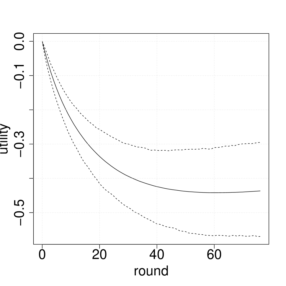
(b) Direct

(c) Mutual

(d) Indirect/Popularity

Figure 2: Tracking vs. Base case

(a) Total

(b) Direct

(c) Mutual

(d) Indirect/Popularity

Figure 3: Random friendships vs. Base case

(a) Total

(b) Direct

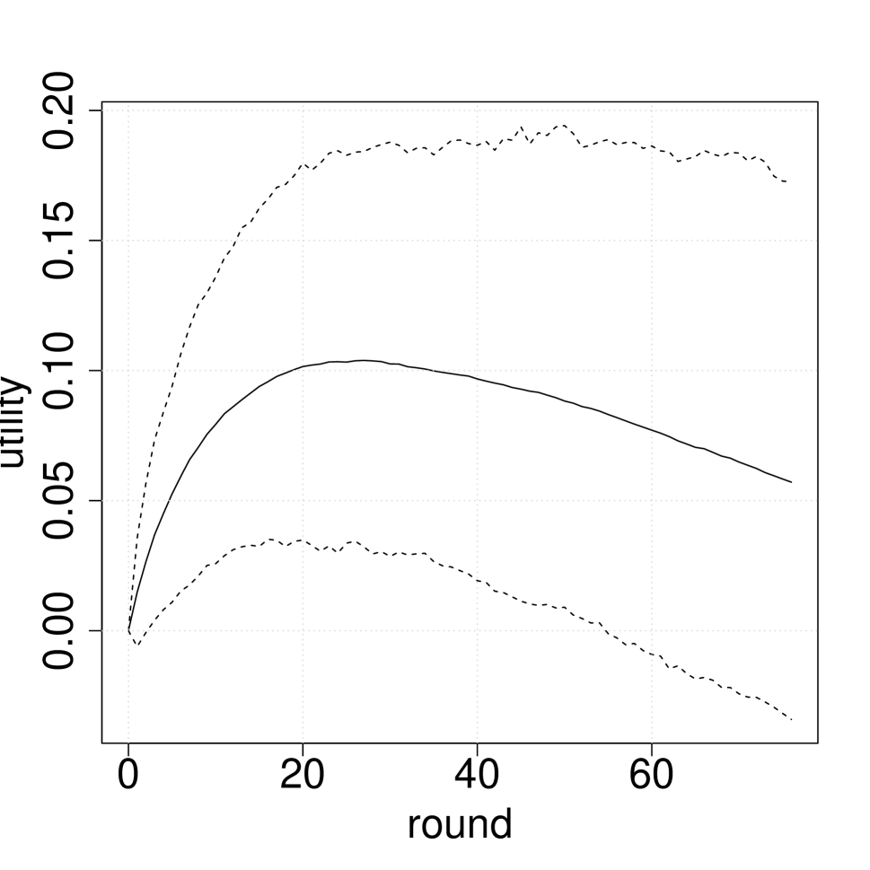
(c) Mutual

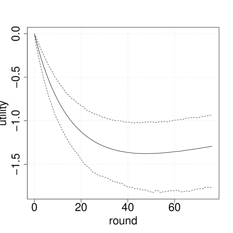
(d) Indirect/Popularity

6 Conclusion

In this article, we studied the identification and estimation of a network formation model that distinguishes between homophily due to preferences and homophily due to meeting opportunities. The model builds upon the algorithm of Mele (2017) by allowing for general classes of utilities and meeting processes. It is also well-grounded in the theoretical literature of network formation (Jackson and Watts, 2002; Jackson, 2010). We provided identification results when a large-support “instrument” is included in preferences (meeting process) and excluded from the meeting process (preferences); and two periods of data from many networks are available. We also discussed a Bayesian estimation procedure that bypasses direct evaluation of the model likelihood – a task that can be computationally unfeasible even for a moderate number of rounds of the network algorithm. All in all, our approach enables users to estimate the counterfactual effects of changes in the meeting technology between agents across time, something previous work could not do.

In the applied section of our article, we studied network formation in elementary schools in Northeastern Brazil. Our results suggest that tracking students according to their cognitive skills improves welfare, though the benefits reduce over time. The effect of this policy can be associated with the structure of the networks. In these classroom networks, homophily due to preferences seems more salient than homophily due to meeting opportunities. This can explain the large positive short-run effect of the tracking policies but the almost zero long-run impact.

As emphasized in Section 3.3, analyzing how restrictions on the relationship between the network structure and payoffs may enable point identification in our setting is an open question that may further enhance the model’s applicability, especially if it allows us to dispense with the exclusion restrictions currently required to identify the model. Another interesting topic for future research is the study of our model under single-network asymptotics, which may be more suitable in some applied settings.

Appendix A Proofs of the main results

In the following, write $N^{k}(g)$, $k\in\mathbb{N}$ and $g\in\mathcal{G}$, for the set of networks that differ from $g$ in exactly $k$ edges.

A.1 Proof of Lemma 3.1

Starting from some $w\in N(g_{0})$, $w_{ij}\neq g_{0ij}$, we can identify $\rho_{ij}(g_{0},X^{m}(g))=\lim_{t\to\infty}(\Pi(X\setminus Z_{ij}^{u}(g_{0},w),Z_{ij}^{u}(g_{0},w)=t\vec{r}_{g_{0}w}))_{g_{0}w}$, which is valid under the (conditional) large support assumption. We are then able to identify $u_{i}(w,X_{i}^{u}(w))$ thanks to the normalization on $u_{i}(g_{0},X_{i}^{u}(g_{0}))$. Proceeding in a similar fashion iteratively on $w^{\prime}\in N^{2}(g_{0}),N^{3}(g_{0})\ldots$, we identify all objects.

A.2 Proof of Proposition 3.1

Before presenting the proof of the main identification result in the paper, we present a lemma for the case in which $\tau_{0}=2$. This lemma provides the intuition for the proof of Proposition 3.1. We show identification when $\tau_{0}=2$ to get an idea of how the general case would look. As seen in the proof, the exclusion restriction given by 3.5 could be relaxed in this case, though the latter would then be insufficient for identification when $\tau_{0}>2$.

Lemma A.1.

Suppose Assumptions 2.1, 2.2, 3.1, 3.3, and 3.5 hold. Then, if $\tau_{0}=2$, the model is identified.

Proof.

First notice that $\Pi(X;\theta)^{2}$ takes the form

$$(\Pi(X;\theta)^{2})_{gw}=\begin{cases}\rho_{ij}(g)F_{ij}(g,[w_{ij},g])\rho_{kl}([w_{ij},g])F_{kl}([w_{ij},g],w)+\\ +\rho_{kl}(g)F_{kl}(g,[w_{kl},g])\rho_{ij}([w_{kl},g])F_{ij}([w_{kl},g],w)&\text{if }w\in N^{2}(g),w_{ij}\neq g_{ij},w_{kl}\neq g_{kl}\\ \Pi_{gg}\rho_{ij}(g)F_{ij}(g,w)+\rho_{ij}(g)F_{ij}(g,w)\Pi_{ww}&\text{if }w\in N(g),w_{ij}\neq g_{ij}\\ \Pi_{gg}\Pi_{gg}+\sum_{s\in N(g)}\Pi_{gs}\Pi_{sg}&\text{if }g=w\\ 0&\text{otherwise}\end{cases}\,.$$ (9)

Fix $g\in\mathcal{G}$, $w\in N(g)$, $g_{ij}\neq w_{ij}$. By driving $F_{ij}(g,w)\to 1$ and $F_{pq}(g,m)\to 0$ for all $m\in N(g)\setminus\{w\}$, $g_{pq}\neq m_{pq}$, the term $(\Pi^{2})_{gg}$ identifies

$$\lim_{t^{*}}(\Pi^{2})_{gg}=(1-\rho_{ij}(g))^{2}\,,$$

where $\lim_{t^{*}}$ is shorthand for the appropriate limit. Since $\lim_{t^{*}}(\Pi^{2})_{gg}\in[0,1]$, we can uniquely solve for $\rho_{ij}(g)$, thus establishing identification of $\rho_{ij}(g)$. Next, by taking $F_{pq}(g,m)\to 0$ for all $m\in N(g)\setminus\{w\}$, $F_{pq}(w,m)\to 0$ for all $m\in N(w)\setminus\{g\}$, the term $\Pi_{gw}$ identifies

$$\lim_{t^{**}}\Pi_{gw}=(1-\rho_{ij}(g)F_{ij}(g,w))\rho_{ij}(g)F_{ij}(g,w)+\rho_{ij}(g)F_{ij}(g,w)(1-\rho_{ij}(w)F_{ij}(w,g))=$$

$$\rho_{ij}(g)F_{ij}(g,w)(2-\rho_{ij}(w)+(\rho_{ij}(w)-\rho_{ij}(g))F_{ij}(g,w))\,,$$

where $\lim_{t^{**}}$ is shorthand for the appropriate limit. Since the right-hand term is strictly increasing in $F_{ij}(g,w)$, the “true” $F_{ij}(g,w)$ uniquely solves the equation, thus establishing identification. ∎

Next we present the proof of Proposition 3.1:

Proof of Proposition 3.1.

Fix $g\in\mathcal{G}$, $w\in N(g)$, $g_{ij}\neq w_{ij}$. Observe that

$$(\Pi^{\tau_{0}})_{gg}=\sum_{m\in N(g)\cup\{g\}}(\Pi^{\tau_{0}-1})_{gm}\Pi_{mg}\,.$$

We first prove the following claim:

Claim.

Under a limit which drives $F_{pq}(w,m)\to 0$ for all $m\in N(w)$, $m_{pq}\neq w_{pq}$, and $F_{kl}(g,s)\to 0$ for all $s\in N(g)\setminus\{w\}$, $s_{kl}\neq g_{kl}$, we have $\lim_{t^{*}}(\Pi^{\tau_{0}})_{gg}=(1-\rho_{ij}(g))^{\tau_{0}}$, where $\lim_{t^{*}}$ is shorthand for the appropriate limit.

Proof.

The case $\tau_{0}=1$ is readily verified by driving $F_{kl}(g,s)\to 0$ for all $s\in N(g)\setminus\{w\}$, $s_{kl}\neq g_{kl}$ and $F_{ij}(g,w)\to 1$. For $\tau_{0}>1$, we begin by noticing that we may drive $(\Pi^{\tau_{0}-1})_{gm}\to 0$ for all $m\in N(g)\setminus\{w\}$. Since $m$ and $g$ differ in exactly one edge (say, $m_{pq}\neq g_{pq}$), a transition in edge $pq$ must appear in every summand in $(\Pi^{\tau_{0}-1})_{gm}$. Indeed, $(\Pi^{\tau_{0}-1})_{gm}$ sums over all possible transitions in edge $pq$ from value $g_{pq}$ to $m_{pq}$ in $\tau_{0}-1$ rounds. Put another way, for each summand in $(\Pi^{\tau_{0}-1})_{gm}$, there exists $t\in\{0,1\ldots\tau_{0}-2\}$, $g^{t}_{pq}=g_{pq}$ and $g^{t+1}_{pq}=m_{pq}$. Fix a summand in $(\Pi^{\tau_{0}-1})_{gm}$. We analyze the following cases:

1. There exists $t\in\{0,1\ldots\tau_{0}-2\}$, $g^{t}_{pq}=g_{pq}$, $g^{t+1}_{pq}=m_{pq}$ and $g^{t}=g$. In this case, by taking $F_{pq}(g,m)\to 0$, we drive the summand to 0.

2. For all $t\in\{0,1\ldots\tau_{0}-2\}$ such that $g^{t}_{pq}=g_{pq}$, $g^{t+1}_{pq}=m_{pq}$, we have $g^{t}\neq g$. Take $t^{*}$ to be the smallest $t$ satisfying the above. Observe that $t^{*}>0$, as $g^{0}=g$ (we always start at $g$). Since $g^{t^{*}}\neq g$, there exists $t^{\prime}<t^{*}$, $g^{t^{\prime}}=g$ and $g^{t^{\prime}+1}=z$, $z\in N(g)$. If there exists some $t^{\prime}$ satisfying this property such that $z\neq w$ (with $g_{kl}\neq z_{kl}$), then driving $F_{kl}(g,z)\to 0$ vanishes the term. If, for all such $t^{\prime}$, $z=w$, take $t^{**}$ to be the maximum of $t^{\prime}$. Observe that $t^{**}<t^{*}$. If $g^{t^{*}}=w$, we may safely drive $F_{pq}(w,[m_{pq},w_{-pq}])\to 0$. If not, then $t^{**}+1<t^{*}$ and there exists a transition from $w$ to some element in $N(w)$ which we can safely drive to 0.

Since the above argument holds, irrespective of the summand (the common limit will vanish all terms), we conclude $(\Pi^{\tau_{0}-1})_{gm}\to 0$. Since $F_{ij}(g,w)\to 1$, $\lim_{t^{*}}(\Pi^{\tau_{0}-1})_{gw}\Pi_{wg}=0$. The common limit in the statement of the claim thus leaves us with

$$\lim_{t^{*}}(\Pi^{\tau_{0}})_{gg}=\lim_{t^{*}}(\Pi^{\tau_{0}-1})_{gg}\lim_{t^{*}}(\Pi)_{gg}=\lim_{t^{*}}(\Pi^{\tau_{0}-1})_{gg}(1-\rho_{ij}(g))\,,$$

Induction then yields the desired result. ∎

Since $\lim_{t^{*}}(\Pi^{\tau_{0}})_{gg}\in[0,1]$, we can uniquely solve for $\rho_{ij}(g)$, thus establishing identification.

Next, we proceed to identification of $F_{ij}(g,w)$. Note that

$$(\Pi^{\tau_{0}})_{gw}=\sum_{m\in N(w)\cup\{w\}}(\Pi^{\tau_{0}-1})_{gm}\Pi_{mw}\,.$$

We then prove the following claim:

Claim.

Under a limit which drives $F_{pq}(w,m)\to 0$ for all $m\in N(w)\setminus\{g\}$, $m_{pq}\neq w_{pq}$, and $F_{kl}(g,s)\to 0$ for all $s\in N(g)\setminus\{w\}$, $s_{kl}\neq g_{kl}$:

$$\lim_{t^{**}}(\Pi^{\tau_{0}})_{gw}=\lim_{t^{**}}(\Pi^{\tau_{0}-1})_{gg}\rho_{ij}(g)F_{ij}(g,w)+\lim_{t^{**}}(\Pi^{\tau_{0}-1})_{gw}(1-\rho_{ij}(w)F_{ij}(w,g))\,,$$

where $\lim_{t^{**}}$ is shorthand for the appropriate limit. We also have that, under such a limit,

$$\lim_{t^{**}}(\Pi^{\tau_{0}})_{gw}+\lim_{t^{**}}(\Pi^{\tau_{0}})_{gg}=1\,.$$

Proof.

For $\tau_{0}=1$, we have

$$\lim_{t^{**}}(\Pi)_{gw}=\rho_{ij}(g)F_{ij}(g,w)\,,$$

$$\lim_{t^{**}}(\Pi)_{gg}=(1-\rho_{ij}(g)F_{ij}(g,w))\,.$$

These expressions follow directly from the limit being taken and equation (2).

Consider next the case $\tau_{0}>1$. The limit in the statement of the lemma drives $(\Pi^{\tau_{0}-1})_{gm}\to 0$ for all $m\in N(w)\setminus\{g\}$. Indeed, if $m\in N(w)\setminus\{g\}$, then $m\in N^{2}(g)$. Recall that $(\Pi^{\tau_{0}-1})_{gm}$ sums over all possible transitions from $g$ to $m$ in $\tau_{0}-1$ rounds. Fix a summand in $(\Pi^{\tau_{0}-1})_{gm}$. If a transition from $g$ occurs at pair $(a,b)\in\mathcal{M}$, $(a,b)\neq(i,j)$, then the limit vanishes the term. If all transitions from $g$ occur at pair $(i,j)$ (i.e. $g$ only transitions to $w$), a transition from $w$ must occur, since $m\in N^{2}(g)$. If $w$ only transitions to $g$, then either $m=g$ or $m=w$, which is not true. Therefore, there exists a transition from $w$ to some $z\in N(w)\setminus\{g\}$, so we can vanish the summand. The limit in the statement thus drives the term $(\Pi^{\tau_{0}-1})_{gm}$ to zero.

From the above discussion, we thus get

$$\lim_{t^{**}}(\Pi^{\tau_{0}})_{gw}=\lim_{t^{**}}(\Pi^{\tau_{0}-1})_{gg}\Pi_{gw}+\lim_{t^{**}}(\Pi^{\tau_{0}-1})_{gw}\Pi_{ww}=$$

$$\lim_{t^{**}}(\Pi^{\tau_{0}-1})_{gg}\rho_{ij}(g)F_{ij}(g,w)+\lim_{t^{**}}(\Pi^{\tau_{0}-1})_{gw}(1-\rho_{ij}(w)F_{ij}(w,g))\,,$$

which establishes the first part of the claim.

Next, under the limit in the statement of the claim

$$\lim_{t^{**}}(\Pi^{\tau_{0}})_{gg}=\lim_{t^{**}}(\Pi^{\tau_{0}-1})_{gg}(1-\rho_{ij}(g)F_{ij}(g,w))+\lim_{t^{**}}(\Pi^{\tau_{0}-1})_{gw}\rho_{ij}(w)F_{ij}(w,g)\,.$$

This follows from observation that, in the proof of the previous claim, we can still drive $(\Pi^{\tau_{0}-1})_{gm}\to 0$ for all $m\in N(g)\setminus\{w\}$ even though $F_{ij}(g,w)$ does not vanish. We are thus left with the terms related to staying in $g$ or transitioning to $w$ in $\tau_{0}-1$ rounds.

Finally, the second part of the claim can be asserted by noticing that $\lim_{t^{**}}(\Pi)_{gw}+\lim_{t^{**}}(\Pi)_{gg}=1$ and applying this fact inductively on the expression for $\lim_{t^{**}}(\Pi^{\tau_{0}})_{gw}+\lim_{t^{**}}(\Pi^{\tau_{0}})_{gg}=\lim_{t^{**}}(\Pi^{\tau_{0}-1})_{gw}+\lim_{t^{**}}(\Pi^{\tau_{0}-1})_{gg}$. ∎

To establish identification of $F_{ij}(g,w)$, we need to show that the expression for $\lim_{t^{**}}(\Pi^{\tau_{0}})_{gw}$ is strictly increasing in $(0,1)$ as a function of $F_{ij}(g,w)$. Denoting by $D_{F_{ij}(g,w)}\lim_{t^{**}}(\Pi^{\tau_{0}})_{gw}$ the derivative of $\lim_{t^{**}}(\Pi^{\tau_{0}})_{gw}$ as a function of $F_{ij}(g,w)$, we get

$$D_{F_{ij}(g,w)}\lim_{t^{**}}(\Pi^{\tau_{0}})_{gw}=D_{F_{ij}(g,w)}\lim_{t^{**}}(\Pi^{\tau_{0}-1})_{gw}(1-\rho_{ij}(w)+(\rho_{ij}(w)-\rho_{ij}(g))F_{ij}(g,w))$$

$$+\rho_{ij}(g)(1-\lim_{t^{**}}(\Pi^{\tau_{0}-1})_{gw})+\rho_{ij}(w)\lim_{t^{**}}(\Pi^{\tau_{0}-1})_{gw}\,,$$

where we use that $\lim_{t^{**}}(\Pi^{\tau_{0}})_{gw}+\lim_{t^{**}}(\Pi^{\tau_{0}})_{gg}=1$ and $F_{ij}(g,w)+F_{ij}(w,g)=1$. By noticing $\rho_{ij}(g)(1-\lim_{t^{**}}(\Pi^{\tau_{0}-1})_{gw})+\rho_{ij}(w)\lim_{t^{**}}(\Pi^{\tau_{0}-1})_{gw}\geq\min\{\rho_{ij}(g),\rho_{ij}(w)\}>0$ and applying induction on the fact that $D_{F_{ij}(g,w)}\lim_{t^{**}}(\Pi)_{gw}\geq 0$, we get that the derivative is strictly positive in $(0,1)$, thus showing that the map is invertible and establishing identification of $F_{ij}(g,w)$. ∎

A.3 Proof of Lemma 4.1

Proof.

Consider the event $\{\hat{\tau}\to\tau_{0}\}^{\complement}$. Observe that $\{\hat{\tau}\to\tau_{0}\}^{\complement}=\cap_{c\in\mathbb{N}}\{\lVert G^{T_{1}}_{c}-G^{T_{0}}_{c}\rVert_{F}<\tau_{0}\}$. Fix $k\in\mathbb{N}$ and notice that

$$\mathbb{P}\left[\cap_{c=1}^{k}\{\lVert G^{T_{1}}_{c}-G^{T_{0}}_{c}\rVert_{F}<\tau_{0}\}\right]=\phi^{k}\,,$$

where $\phi$ is the ex-ante (unconditional) probability that $G^{T_{1}}_{c}$ differs from $G^{T_{0}}_{c}$ in strictly less than $\tau_{0}$ edges. Since $\mathbb{P}[\lVert G^{T_{1}}_{c}-G^{T_{0}}_{c}\rVert_{F}=\tau_{0}]\in(0,1)$ (which follows from 2.1, 2.2, and 3.2), we have $\phi\in(0,1)$. Passing $k$ to the limit and using continuity of $\mathbb{P}$ from above, we conclude the desired result. ∎

It is apparent from the proof above that it is possible extend the result of Lemma 4.1 in order to allow for a sequence of independent observations stemming from a game with common $\tau_{0}$, but allowing utilities, the meeting process, the distribution of covariates and the number of players to vary between networks. In this case, we must restrict the distribution of covariates, utilities, the meeting process and the number of players to not shift excessively to regions where the probability of the network changing by strictly less than $\tau_{0}$ edges is high. Formally, the proof would change as the ex-ante probability would now depend on $c$, i.e. we would have $\prod_{c=1}^{k}\phi_{c}$ in the formula. If $\limsup_{c\to\infty}\phi_{c}<1$, we would get the same result. Observe this implies $\limsup_{c\to\infty}\mathbb{P}[N_{c}(N_{c}-1)\geq\tau_{0}]>0$.

See pages - of supplementalappendix.pdf

References

- Aguirregabiria and Mira (2010) Aguirregabiria, V. and P. Mira (2010). Dynamic discrete choice structural models: A survey. Journal of Econometrics 156(1), 38 – 67. Structural Models of Optimization Behavior in Labor, Aging, and Health.
- Amemiya (1985) Amemiya, T. (1985). Advanced Econometrics. Harvard University Press.
- Badev (2021) Badev, A. (2021). Nash equilibria on (un)stable networks. Econometrica 89(3), 1179–1206.
- Bajari et al. (2010) Bajari, P., H. Hong, and S. P. Ryan (2010). Identification and estimation of a discrete game of complete information. Econometrica 78(5), 1529–1568.
- Barthelmé et al. (2018) Barthelmé, S., N. Chopin, and V. Cottet (2018). Divide and conquer in ABC: Expectation-propagation algorithms for likelihood-free inference. Handbook of Approximate Bayesian Computation, 415–34.
- Barthelmé and Chopin (2014) Barthelmé, S. and N. Chopin (2014). Expectation propagation for likelihood-free inference. Journal of the American Statistical Association 109(505), 315–333.
- Battaglini et al. (2021) Battaglini, M., E. Patacchini, and E. Rainone (2021). Endogenous social interactions with unobserved networks. The Review of Economic Studies.
- Blum (2010) Blum, M. G. B. (2010). Approximate bayesian computation: A nonparametric perspective. Journal of the American Statistical Association 105(491), 1178–1187.
- Bramoullé et al. (2012) Bramoullé, Y., S. Currarini, M. O. Jackson, P. Pin, and B. W. Rogers (2012). Homophily and long-run integration in social networks. Journal of Economic Theory 147(5), 1754 – 1786.
- Centola (2011) Centola, D. (2011). An experimental study of homophily in the adoption of health behavior. Science 334(6060), 1269–1272.
- Chandrasekhar (2016) Chandrasekhar, A. (2016). Econometrics of network formation. In The Oxford Handbook of the Economics of Networks, pp. 303–357. Oxford University Press.
- Chandrasekhar and Jackson (2021) Chandrasekhar, A. G. and M. O. Jackson (2021). A network formation model based on subgraphs.
- Chetty et al. (2022a) Chetty, R., M. O. Jackson, T. Kuchler, J. Stroebel, N. Hendren, R. B. Fluegge, S. Gong, F. Gonzalez, A. Grondin, M. Jacob, et al. (2022a). Social capital i: measurement and associations with economic mobility. Nature 608(7921), 108–121.
- Chetty et al. (2022b) Chetty, R., M. O. Jackson, T. Kuchler, J. Stroebel, N. Hendren, R. B. Fluegge, S. Gong, F. Gonzalez, A. Grondin, M. Jacob, et al. (2022b). Social capital ii: determinants of economic connectedness. Nature 608(7921), 122–134.
- Christakis et al. (2020) Christakis, N., J. Fowler, G. W. Imbens, and K. Kalyanaraman (2020). An empirical model for strategic network formation. In B. Graham and A. de Paula (Eds.), The Econometric Analysis of Network Data, Chapter Chapter 6, pp. 123–148. Academic Press.
- Colas and Morehouse (2022) Colas, M. and J. M. Morehouse (2022). The environmental cost of land-use restrictions. Quantitative Economics 13(1), 179–223.
- Currarini et al. (2009) Currarini, S., M. O. Jackson, and P. Pin (2009). An economic model of friendship: Homophily, minorities, and segregation. Econometrica 77(4), 1003–1045.
- Currarini et al. (2010) Currarini, S., M. O. Jackson, and P. Pin (2010). Identifying the roles of race-based choice and chance in high school friendship network formation. Proceedings of the National Academy of Sciences 107(11), 4857–4861.
- de Paula (2017) de Paula, A. (2017). Econometrics of network models. In B. Honoré, A. Pakes, M. Piazzesi, and L. Samuelson (Eds.), Advances in Economics and Econometrics: Eleventh World Congress, Econometric Society Monographs, pp. 268–323. Cambridge University Press.
- de Paula et al. (2018) de Paula, Á́., S. Richards-Shubik, and E. Tamer (2018). Identifying preferences in networks with bounded degree. Econometrica 86(1), 263–288.
- Frazier et al. (2018) Frazier, D. T., G. M. Martin, C. P. Robert, and J. Rousseau (2018). Asymptotic properties of approximate Bayesian computation. Biometrika 105(3), 593–607.
- Goldsmith-Pinkham and Imbens (2013) Goldsmith-Pinkham, P. and G. W. Imbens (2013). Social networks and the identification of peer effects. Journal of Business & Economic Statistics 31(3), 253–264.
- Graham (2016) Graham, B. S. (2016). Homophily and transitivity in dynamic network formation. Working Paper 22186, National Bureau of Economic Research.
- Graham (2017) Graham, B. S. (2017). An econometric model of network formation with degree heterogeneity. Econometrica 85(4), 1033–1063.
- Higham and Lin (2011) Higham, N. J. and L. Lin (2011). On pth roots of stochastic matrices. Linear Algebra and its Applications 435(3), 448 – 463. Special Issue: Dedication to Pete Stewart on the occasion of his 70th birthday.
- Hobert (2011) Hobert, J. P. (2011). Chapter 10 the data augmentation algorithm: Theory and methodology. In Handbook of Markov Chain Monte Carlo, pp. 253–294. CRC Press.
- Horn and Johnson (2012) Horn, R. A. and C. R. Johnson (2012). Matrix Analysis. Cambridge University Press.
- Hsieh and Lee (2016) Hsieh, C.-S. and L. F. Lee (2016). A social interactions model with endogenous friendship formation and selectivity. Journal of Applied Econometrics 31(2), 301–319.
- Jackson (2010) Jackson, M. (2010). Social and Economic Networks. Princeton University Press.
- Jackson (2021) Jackson, M. O. (2021). Inequality’s economic and social roots: The role of social networks and homophily. SSRN Electronic Journal.
- Jackson and Watts (2002) Jackson, M. O. and A. Watts (2002). The evolution of social and economic networks. Journal of Economic Theory 106(2), 265 – 295.
- Kadelka and McCombs (2021) Kadelka, C. and A. McCombs (2021). Effect of homophily and correlation of beliefs on COVID-19 and general infectious disease outbreaks. PLOS ONE 16(12).
- Li and Racine (2006) Li, Q. and J. S. Racine (2006). Nonparametric Econometrics: Theory and Practice. Princeton University Press.
- Li and Fearnhead (2018) Li, W. and P. Fearnhead (2018). On the asymptotic efficiency of approximate Bayesian computation estimators. Biometrika 105(2), 285–299.
- McFadden (1973) McFadden, D. (1973). Conditional logit analysis of qualitative choice behaviour. In P. Zarembka (Ed.), Frontiers in Econometrics, pp. 105–142. New York, NY, USA: Academic Press New York.
- Mele (2017) Mele, A. (2017). A structural model of dense network formation. Econometrica 85(3), 825–850.
- Newey and McFadden (1994) Newey, W. K. and D. McFadden (1994). Large sample estimation and hypothesis testing. In Handbook of Econometrics, Volume 4, Chapter 36, pp. 2111 – 2245. Elsevier.
- Newey and Smith (2004) Newey, W. K. and R. J. Smith (2004). Higher order properties of gmm and generalized empirical likelihood estimators. Econometrica 72(1), 219–255.
- Norris (1997) Norris, J. R. (1997). Markov Chains. Cambridge Series in Statistical and Probabilistic Mathematics. Cambridge University Press.
- Pinto and Ponczek (2020) Pinto, C. C. d. X. and V. P. Ponczek (2020). The building blocks of skill development. Unpublished.
- Rothenberg (1971) Rothenberg, T. J. (1971). Identification in parametric models. Econometrica 39(3), 577–591.
- Sheng (2020) Sheng, S. (2020). A structural econometric analysis of network formation games through subnetworks. Econometrica 88(5), 1829–1858.
- Sisson and Fan (2011) Sisson, S. A. and Y. Fan (2011). Chapter 12 likelihood-free mcmc. In Handbook of Markov Chain Monte Carlo, pp. 313–338. CRC Press.
- Tamer (2003) Tamer, E. (2003). Incomplete simultaneous discrete response model with multiple equilibria. The Review of Economic Studies 70(1), 147–165.
- Vaart (1998) Vaart, A. W. v. d. (1998). Asymptotic Statistics. Cambridge Series in Statistical and Probabilistic Mathematics. Cambridge University Press.
- Zeng and Xie (2008) Zeng, Z. and Y. Xie (2008). A preference-opportunity-choice framework with applications to intergroup friendship. American Journal of Sociology 114(3), 615–648.