A Strengthened Branch and Bound Algorithm
for the Maximum Common (Connected) Subgraph Problem

Abstract

We propose a new and strengthened Branch-and-Bound (BnB) algorithm for the maximum common (connected) induced subgraph problem based on two new operators, Long-Short Memory (LSM) and Leaf vertex Union Match (LUM). Given two graphs for which we search for the maximum common (connected) induced subgraph, the first operator of LSM maintains a score for the branching node using the short-term reward of each vertex of the first graph and the long-term reward of each vertex pair of the two graphs. In this way, the BnB process learns to reduce the search tree size significantly and improve the algorithm performance. The second operator of LUM further improves the performance by simultaneously matching the leaf vertices connected to the current matched vertices, and allows the algorithm to match multiple vertex pairs without affecting the solution optimality. We incorporate the two operators into the state-of-the-art BnB algorithm McSplit, and denote the resulting algorithm as McSplit+LL. Experiments show that McSplit+LL outperforms McSplit+RL, a more recent variant of McSplit using reinforcement learning that is superior than McSplit.

1 Introduction

Graphs are important data structures that can be used to model many real-world problems. One of the most basic graph problems is to measure the similarity of graphs. Given two graphs $G_{0}$ and $G_{1}$, the Maximum Common induced Subgraph (MCS) aims to find an induced subgraph $G_{0}^{\prime}$ in $G_{0}$ and an induced subgraph $G_{1}^{\prime}$ in $G_{1}$ such that $G_{0}^{\prime}$ and $G_{1}^{\prime}$ are isomorphic and the number of vertices of $G_{0}^{\prime}$ and $G_{1}^{\prime}$ is maximized. The vertices of $G_{0}^{\prime}$ are said to be matched with the vertices of $G_{1}^{\prime}$. MCS has a variant called the Maximum Common Connected induced Subgraph (MCCS), which further requires the induced subgraph to be connected. These problems are widely applied in various domains, such as biochemistry Giugno et al. (2013); Bonnici et al. (2013), cheminformatics Raymond and Willett (2002); Englert and Kovács (2015); Duesbury et al. (2017), compilers Blindell et al. (2015), model checking Sevegnani and Calder (2015), molecular science Ehrlich and Rarey (2011), pattern recognition Solnon et al. (2015), malware detection Bruschi et al. (2006); Park et al. (2013), video and image analysis Shearer et al. (2001); Jiang and Ngo (2003); Hati et al. (2016), etc.

As an NP-hard problem, MCS is computationally very challenging. Many approaches have been proposed for solving MCS and its related problems, which could be mainly divided into two categories: exact algorithms and inexact algorithms. An exact algorithm guarantees to obtain an optimal solution but runs in exponential time in the worst case. It aims to efficiently enumerate the whole search space or reduce the search space without affecting the solution’s optimality. The approaches for exact algorithms include Linear Programming (LP) Bahiense et al. (2012), Branch-and-Bound (BnB) Raymond and Willett (2002); McCreesh et al. (2017); Liu et al. (2020), etc. An inexact algorithm aims to find a near-optimal solution within reasonable computational resources (e.g., time and memory). The approaches for inexact algorithms include heuristics Bonnici et al. (2013); Englert and Kovács (2015); Duesbury et al. (2017) and metaheuristics Choi et al. (2012). Recently, machine learning Shearer et al. (2001) and deep learning  Zanfir and Sminchisescu (2018); Bai et al. (2021) techniques are also adopted for solving MCS.

The BnB algorithms have exhibited high performance for MCS problems. Given a vertex $p$ in $G_{0}$, McSplit McCreesh et al. (2017), one of the state-of-the-art algorithms for MCS, proposes a partition method to efficiently filter the set of candidate vertices of $G_{1}$ that can be matched with $q$, and uses a novel compact candidate set representation to dramatically reduce the memory and computational requirements during the search. McSplit+RL Liu et al. (2020) further improves McSplit using a new branching method based on reinforcement learning.

In this work, we propose two new operators to speed up the BnB process, namely Long-Short Memory (LSM) and Leaf vertex Union Match (LUM). In a BnB process for MCS, the branching consists in first selecting a vertex $p$ from the first graph $G_{0}$, and then matching each candidate vertex $q$ of $G_{1}$ in turn. LSM maintains a score for each $p$ using the short-term reward, and the long-term reward of each branching pair $\langle p,q\rangle$. In this way, the search tree size could be reduced. LUM improves the efficiency in a different way. When a pair of vertices are matched for branching, LUM also matches the leaf vertices connected to the current matched vertices, allowing to reduce the search space while keeping the solution’s optimality.

We implement our two operators on top of McSplit, and design a new and strengthened algorithm called McSplit+LL. We extensively evaluate McSplit+LL on 25,552 instances from diverse applications as McSplit+RL does. Results show that the proposed McSplit+LL clearly outperforms McSplit and McSplit+RL, which are already highly efficient. We also carry out an empirical analysis to give insight on why and how our two proposed operators are effective, suggesting that both of them can reduce the search tree size, so as to improve the efficiency. Besides, the second operator of LUM is general and could be useful for other graph search problems.

2 Problem Definition

Consider a simple (undirected or directed , unlabelled) graph $G=(V,E)$, where $V$ and $E$ represent the vertex set and the edge set, respectively. Two vertices $u,v$ are called adjacent if $(u,v)\in E$, and the degree of a vertex $u$ is the number of its adjacent vertices. An induced subgraph $G^{\prime}=(V^{\prime},E^{\prime})$ of $G$ consists of a vertex subset $V^{\prime}\subseteq V$ and the edges in $E^{\prime}=\{(u,v)\mid\forall u,v\in V^{\prime},(u,v)\in E\}$.

Given two graphs $G_{0}$ and $G_{1}$, if there is an induced subgraph $G_{0}^{\prime}$ of $G_{0}$ and there exists a bijection $\phi:V_{0}^{\prime}$ $\rightarrow V_{1}^{\prime}$, $\Phi(G_{0}^{\prime})$ ($\Phi(G)$ donates a graph that mapping all vertices in $G$ by $\phi$) is also an induced subgraph of $G_{1}$, then we call $\langle G_{0}^{\prime},\Phi(G_{0}^{\prime})\rangle$ is the common induced subgraph of $\langle G_{0},G_{1}\rangle$. Let $V^{\prime}=\{v_{1},v_{2},...,v_{|V^{\prime}|}\}$, the common induced subgraph is also represented as a list of vertex pairs $\{\langle v_{1},\phi(v_{1})\rangle,\langle v_{2},\phi(v_{2})\rangle,...,\langle v_{|V^{\prime}|},\phi(v_{|V^{\prime}|})\rangle\}$

The Maximum Common induced Subgraph (MCS) problem aims to find the common induced subgraph such that the number of its vertices is maximized. In other words, the two induced subgraphs are isomorphic with the maximum vertex cardinality. There is a variant problem of MCS, the Maximum Common Connected induced Subgraph (MCCS) problem, which requires the induced subgraph is connected.

3 Branch and Bound for MCS

This section presents two of the best-performing BnB algorithms for MCS and MCCS, which are McSplit McCreesh et al. (2017) and McSplit+RL Liu et al. (2020). To simplify the algorithm description, we initially assume that the graphs are undirected, as the method is easy to be adapted to handle various extensions of the problem McCreesh et al. (2017).

At each search node, the BnB algorithm first estimates an upper bound of the best solution that can be found in the current subtree. If the upper bound is not larger than the size of the current best solution, the algorithm prunes this branch and backtracks, because any better solution cannot be found under this search node. Otherwise, it selects a new vertex pair to match, updates the current solution and then runs recursively. There are three key issues for implementing the BnB algorithm: 1) estimate the upper bound, 2) design the branching strategy, 3) maintain candidate vertices of the two graphs. To address these issues, McSplit and McSplit+RL proposed label class and a learning based scoring mechanism for the branching nodes, respectively.

Algorithm 1 MCS($\mathcal{D}$, $\alpha$, $\beta$, $\gamma$, $S_{cur}$, $S_{best}$)

Input: A bidomain list $\mathcal{D}$; three heuristic functions $\alpha$, $\beta$ and $\gamma$ for selecting the bidomain, the first matched vertex, and the second matched vertex, respectively; the current maintained solution $S_{cur}$; the best solution found so far $S_{best}$.
Output: The optimal solution $S_{best}$.

1:  $UB$ $\leftarrow$ $\text{overEstimate}(\mathcal{D})$ $+$ $|S_{cur}|$

2:  if $UB\leq|S_{best}|$ then

3:     return $S_{best}$

4:  end if

5:  $\langle V_{l},V_{r}\rangle$ $\leftarrow$ a bidomain by the heuristic $\alpha(\mathcal{D})$

6:  $p$ $\leftarrow$ a vertex obtained by the heuristic $\beta(V_{l})$

7:  $m$ $\leftarrow$ $|V_{r}|$

8:  for i from 1 to $m$ do

9:     $q$ $\leftarrow$ a vertex obtained by the heuristic $\gamma(V_{r})$

10:     $V_{r}$ $\leftarrow$ $V_{r}\setminus\{q\}$

11:     $S_{cur}^{\prime}$ $\leftarrow$ $S_{cur}\cup\{\langle p,q\rangle\}$

12:     if $|S_{cur}^{\prime}|>|S_{best}|$ then

13:        $S_{best}$ $\leftarrow$ $S_{cur}^{\prime}$

14:     end if

15:     $\mathcal{D}^{\prime}$ $\leftarrow$ a new bidomain list obtained by dividing $\mathcal{D}$

16:     $S_{best}$ $\leftarrow$ MCS($\mathcal{D}^{\prime}$, $\alpha$, $\beta$, $\gamma$, $S_{cur}^{\prime}$, $S_{best}$)

17:  end for

18:  $\mathcal{D}^{\prime}$ $\leftarrow$ a new bidomain list obtained by removing $p$ from $\mathcal{D}$

19:  $S_{best}$ $\leftarrow$ MCS($\mathcal{D}^{\prime}$, $\alpha$, $\beta$, $\gamma$, $S_{cur}$, $S_{best}$)

20:  return $S_{best}$

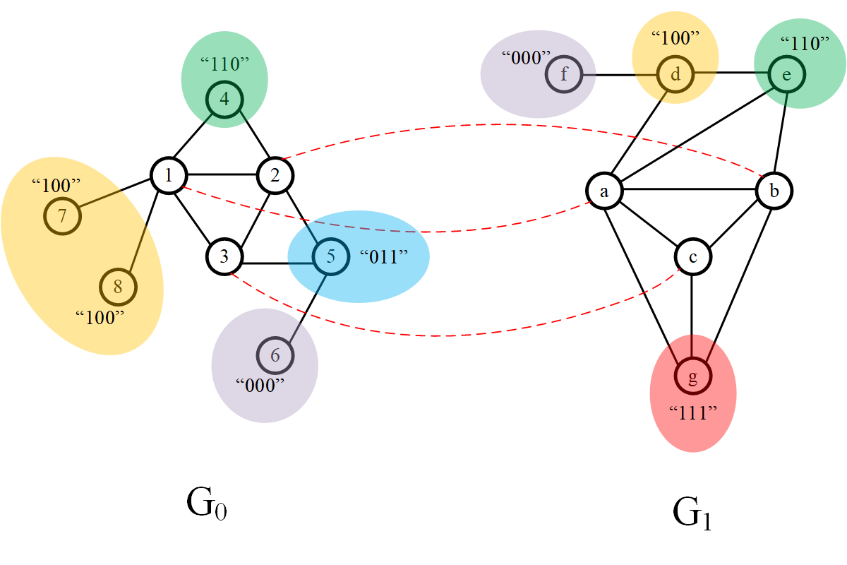
Figure 1: An example to illustrate the concepts of bidomain and label class for MCS. There are three matched vertex pairs $\langle 1,a\rangle$, $\langle 2,b\rangle$ and $\langle 3,c\rangle$. According to the definitions of bidomain and label class, the remaining vertices are divided into three valid bidomains $D$(“000”) $=\langle\{6\},\{f\}\rangle$, $D$(“100”) $=\langle\{7,8\},\{d\}\rangle$ and $D$(“110”) $=\langle\{4\},\{e\}\rangle$, where “0” indicates that the vertex is not adjacent to the corresponding matched vertex and “1” otherwise. Note that $D$(“011”) and $D$(“111”) are invalid bidomains, as they cannot provide any matched vertex pair, and will be removed in the bidomain dividing process.

3.1 The BnB Framework for MCS Problems

McCreesh et al. (2017) proposes a BnB framework for MCS problems, that the current best-performing algorithms McSplit and McSplit+RL both adopt. For two input graphs $G_{0}$ and $G_{1}$, the bidomain structure consists of two vertex sets $\langle V_{l},V_{r}\rangle$, where $V_{l}$ and $V_{r}$ are subsets of $V(G_{0})$ and $V(G_{1})$, respectively. McSplit assigns a label to each of the bidomains. The label indicates that each vertex in the bidomain has the same connectivity to the matched vertices, and is represented by a “01”-string. Therefore the two graphs can be represented as a list of bidomains $\mathcal{D}$ during the search and any vertex pair selected from each bidomain is legal to match. Whenever a vertex pair $\langle p,q\rangle$ matches, each bidomain $\langle V_{l},V_{r}\rangle$ will be divided into two new bidomains $\langle V_{l}^{0},V_{r}^{0}\rangle$ and $\langle V_{l}^{1},V_{r}^{1}\rangle$, where the superscript “0” and “1” indicate the connectivity of the matched vertex pair $\langle p,q\rangle$. See Figure 1 for an illustrative example.

Obviously, a bidomain $\langle V_{l},V_{r}\rangle$ can provide at most $\min(|V_{l}|,|V_{r}|)$ matched vertex pairs. Therefore, the algorithm estimates the upper bound of the bidomain list $\mathcal{D}$ by the following equation:

$$\text{overEstimate}(\mathcal{D})=\sum_{\langle V_{l},V_{r}\rangle\in\mathcal{D}}\min(|V_{l}|,|V_{r}|)$$ (1)

Then, we introduce the flow of BnB algorithm based on the depth-first search for MCS, as depicted in Algorithm 1. The call of MCS($\{\langle V(G_{0}),V(G_{1})\rangle\}$, $\alpha$, $\beta$, $\gamma$, $\emptyset$, $\emptyset$) returns a maximum common induced subgraph of $G_{0}$ and $G_{1}$ where $\alpha$, $\beta$ and $\gamma$ are the heuristics. At each search node, the algorithm calculates the upper bound assisted by Eq. 1 and uses the upper bound to determine whether it can find a better solution from this search node. If there exists no better solution from this node, the algorithm prunes and backtracks. Then it selects a bidomain $\langle V_{l},V_{r}\rangle$ from the current bidomain list $\mathcal{D}$ by heuristic $\alpha$ and picks a vertex $p$ from $V_{l}$ by heuristic $\gamma$. The algorithm enumerates all the vertices in $V_{r}$ to match with the vertex $p$ where the order of enumeration is decided by heuristic $\gamma$. When a vertex pair $\langle p,q\rangle$ is matched, the algorithm appends the matched pair to the current solution, updates the best solution, and obtains a new bidomain list $\mathcal{D}^{\prime}$ by dividing the current bidomain list $\mathcal{D}$ by $\langle p,q\rangle$. Afterwards, the algorithm runs recursively with the new bidomain list $\mathcal{D}^{\prime}$. After enumerating all the possible matched vertex pairs of $p$, the rest of the configuration is that vertex $p$ does not appear in the matched vertex pair list, thus the algorithm removes vertex $p$ from the current bidomain list and runs recursively.

3.2 McSplit and McSplit+RL

There are three heuristics $\alpha$, $\beta$ and $\gamma$ that represent the strategy of selecting the bidomain, selecting the first matched vertex and the order of enumerating the second matched vertex, respectively. These heuristics are the essential components in the BnB framework, that lead to different BnB algorithms.

McSplit McCreesh et al. (2017) implements the three heuristics as follows:

• $\alpha$: McSplit defines the value of $\max(|V_{l}|,|V_{r}|)$ as the size of the bidomain. It selects a bidomain with the smallest size from the bidomain list and uses the largest vertex degree in $V_{l}$ to break ties.

• $\beta$: Picks the largest degree vertex from $V_{l}$ as the first matched vertex.

• $\gamma$: Enumerates the second matched vertex in $V_{r}$ in decreasing order of vertex degree.

McSplit+RL Liu et al. (2020) introduces a learning based branching heuristic, so as to choose a branching pair with the largest bound reduction and reach the pruning condition as early as possible. McSplit+RL regards the BnB algorithm as an agent and a vertex pair selection as an action. When a vertex pair $\langle p,q\rangle$ is matched, and the current bidomain list $\mathcal{D}$ is divided into $\mathcal{D}^{\prime}$, McSplit+RL uses the estimated bound reduction of the bidomain list as the reward $r(p,q)$ of taking action $\langle p,q\rangle$.

$$r(p,q)=\text{overEstimate}(\mathcal{D})-\text{overEstimate}(\mathcal{D}^{\prime}).$$ (2)

McSplit+RL maintains two score lists $S_{0}(\cdot)$ and $S_{1}(\cdot)$ for each vertex in $G_{0}$ and $G_{1}$, records the accumulated rewards of each vertex. Specifically, update the score lists as follows:

$$S_{0}(p) \leftarrow S_{0}(p)+r(p,q)$$ (3)

$$S_{1}(q) \leftarrow S_{1}(q)+r(p,q)$$

Then McSplit+RL replaces heuristics $\beta$ and $\gamma$ based on the two score lists as follows:

• $\beta$: Picks a vertex $p$ with the largest score $S_{0}(p)$ from $V_{l}$ as the first matched vertex.

• $\gamma$: Enumerates the second matched vertex $q$ in $V_{r}$ in decreasing order of the $S_{1}(q)$ score.

4 The Proposed McSplit+LL Algorithm

We first analyze the limits of the existing branching heuristic, and then we propose a new and strengthened branching heuristic called Long-Short Memory (LSM). Furthermore, we propose a Leaf vertex Union Match (LUM) method for the vertex-vertex mapping based algorithm. We implement both LSM and LUM on top of McSplit, and call the resulting new algorithm McSplit+LL.

4.1 Further Discussion on McSplit(+RL)

In McSplit, the selecting vertex pair heuristics $\beta$ and $\gamma$ are straightforward and not adaptive, hence its branching strategy may not be the best choice to minimize the search tree size.

In McSplit+RL, the main idea for the branching is to use the bound reduction to evaluate each vertex.Then it selects the vertex with the largest evaluation score to match, aiming to reduce the bound as much as possible and quickly reach the pruning condition. The score is accumulated during the entire BnB algorithm, i.e., it is the summation of all the historical evaluation values. However, with the number of recursion and backtracking increases, the situation of the current solution and unmatched vertices (the bidomains) in the two graphs have changed drastically. Accumulating the scores evenly causes a bias caused by a large proportion of historical evaluation values when the current configuration differs from the historical configuration. Hence, we need a mechanism that can reasonably eliminate the influence of the historical evaluations.

4.2 Long-Short Memory Branching Heuristic

To overcome the limits of existing BnB methods, we apply the reinforcement learning method in McSplit+RL to evaluate the benefit of matching each vertex on the reduction of the search tree size, and further propose a mechanism to eliminate the historical evaluations by decaying part of the evaluation values when they reach a predetermined upper limit.

Our method maintains a score list $S_{0}(\cdot)$ as McSplit+RL does, and further maintains a score table $S_{t}(p,q)$ of each vertex pair $\langle p,q\rangle$ simultaneously. The initial value of the score table $S_{t}(p,q)$ is set to 0 for each vertex pair $\langle p,q\rangle$. Whenever action $\langle p,q\rangle$ is performed, $S_{t}(p,q)$ will be updated by the following formula:

$$S_{t}(p,q)=S_{t}(p,q)+r(p,q).$$ (4)

Our method replaces the $\gamma$ heuristic in McSplit+RL with:

• $\gamma$: Enumerates the second matched vertex $q$ in $V_{r}$ in decreasing order of the $S_{t}(p,q)$ score.

Before introducing our decaying mechanism, we first provide insights on the scoring mechanism. Firstly, score $S_{0}(p)$ is accumulated by reward $r(p,q)$ where vertex $p$ and $q$ are in the same bidomain. The bound reduction is seriously influenced by matching to which vertex $q$, and the bidomains are changed frequently that means the vertices matched to $p$ are very dynamic. It will lead the evaluation score to be outdated quickly. Thus, using the score $S_{0}(p)$ to evaluate the bound reduction of taking action $\langle p,q\rangle$ is very inaccurate. Secondly, the evaluation score on vertex pair $S_{t}(p,q)$ records the reward $r(p,q)$ properly, which is more accurate than $S_{0}(p)$. So the historical rewards accumulated by $S_{t}(p,q)$ have significant reference value. So we propose a LSM strategy to make the score list $S_{0}(\cdot)$ focus on the short-term reward, and the score table $S_{t}(\cdot,\cdot)$ focus on the long-term reward.

In LSM, a short-term threshold value $T_{s}$ ($10^{5}$ by default) and a long-term threshold value $T_{l}$ ($10^{9}$ by default) are used to implement our mechanism. At each search node, when the algorithm is branching and the score $S_{0}(p)$ and $S_{t}(p,q)$ are updated, if score $S_{0}(p)$ is greater than $T_{s}$, then all the scores in the score list $S_{0}(\cdot)$ decay to a half. And we regard the score table $S_{t}(\cdot,\cdot)$ as $|V(G_{0})|$ score lists, i.e., $S_{t}(\cdot,\cdot)=S_{t}(v_{1},\cdot),S_{t}(v_{2},\cdot),...,S_{t}(v_{|V(G_{0})|},\cdot)$. If score $S_{t}(p,q)$ is greater than $T_{l}$, then all the scores in the score list $S_{t}(p,\cdot)$ decay to a half. The decaying operation in each score list of the score table is independent.

4.3 Leaf Vertex Union Match

We first provide a definition of the leaf vertex of an undirected graph. A vertex is regarded as a leaf if it is adjacent to exactly one vertex in the graph and the leaves of vertex $u$ indicate the leaves adjacent to $u$. Then, we provide the main theory to support our LUM strategy.

Theorem 1.

In the BnB framework, when a vertex pair $\langle p,q\rangle$ is matched, we can match as many leaf pairs as possible from the unmatched leaves of vertex $p$ and $q$ without affecting the solution’s optimality.

Proof.

Assume the current solution has $k$ matched vertex pairs and the $i$-th pair is $\langle p,q\rangle$. According to the label class definition in Section 3.1, the labels of the unmatched leaves of $p$ and $q$ are all the same as “0…010…0” which has exactly one “1” in the $i$-th position, because the leaves are only adjacent to the vertex $p$ and $q$ respectively. Thus, these leaves are always partitioned in the same bidomain. It guarantees that no matter what the matching configuration of other vertices is, the leaves of $p$ and leaves of $q$ are always legal to match as long as $p$ and $q$ match together. If arbitrary pair of leaves are matched, all the remaining unmatched vertices are not adjacent to both matched leaves. Matching any leaf pair does not divide a new bidomain from the current bidomain list. Therefore, such an operation does not affect the solution’s optimality of the BnB algorithm for MCS. ∎

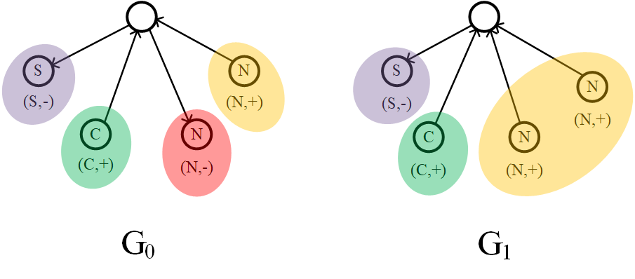
Figure 2: An example to illustrate the leaf attribute of LUM for a general situation. It shows two directed and labelling graphs $G_{0}$ and $G_{1}$ (only vertices are labelled, thus we omit the edge label in the leaf attribute), each leaf attribute is given below the leaf. The leaf attribute $(A,\pm)$ represents the vertex label and the direction of arc connected to the leaf respectively. Sign $+$ means the leaf is the head of the arc and sign $-$ means the leaf is the tail of the arc. There are at most three leaf pairs that can be provided in this example.

Our LUM strategy can be extended to general graph matching problems. Consider a directed and labelling graph, where both vertices and arcs are labelled. Let $L_{v}=\{a_{1},a_{2},a_{3},...\}$ and $L_{e}=\{b_{1},b_{2},b_{3},...\}$ represent the vertex label set and the arc label set, respectively. We give each leaf an attribute $(a_{i},\pm b_{j})$ where $a_{i}$ is the label of vertex, $b_{j}$ is the label of arc connected to the leaf and the sign represents the direction of arc ($+$ means leaf is head, $-$ means leaf is tail). We partition the leaves into different groups according to the attributes. Leaves in the corresponding group can be matched, therefore it can match as many leaf pairs as possible in each group. We also provide an example as shown in Figure 2. Note that the leaf grouping is independent of the bidomain dividing.

5 Experiments

We compare our proposed McSplit+LL algorithm with McSplit+RL Liu et al. (2020), which is the state-of-the-art BnB exact algorithm for MCS. We tested the algorithms on both the MCS and MCCS problems. The experimental results show that McSplit+LL outperforms McSplit+RL for solving these problems. Further ablation studies show the effectiveness of our proposed methods, including LSM branching heuristic and LUM strategy.

5.1 Experimental Setup

Experiments were performed on a server with Intel® Xeon® E5-2650 v3 CPU and 256GBytes RAM. The algorithms were implemented in C++ and compiled using g++ 5.4.0. The cutoff time is set to 1800 seconds for each instance, which is the same as in Liu et al. (2020).

There are two parameters, $T_{s}$ and $T_{l}$ for the LSM branching heuristic. We sample some instances solved between 10 to 30 minutes and the parameter tuning domain is set to $10^{k},k\in[2,9]$. Finally, the default setting of two parameters $T_{s}$ and $T_{l}$ are $10^{5}$ and $10^{9}$, respectively.

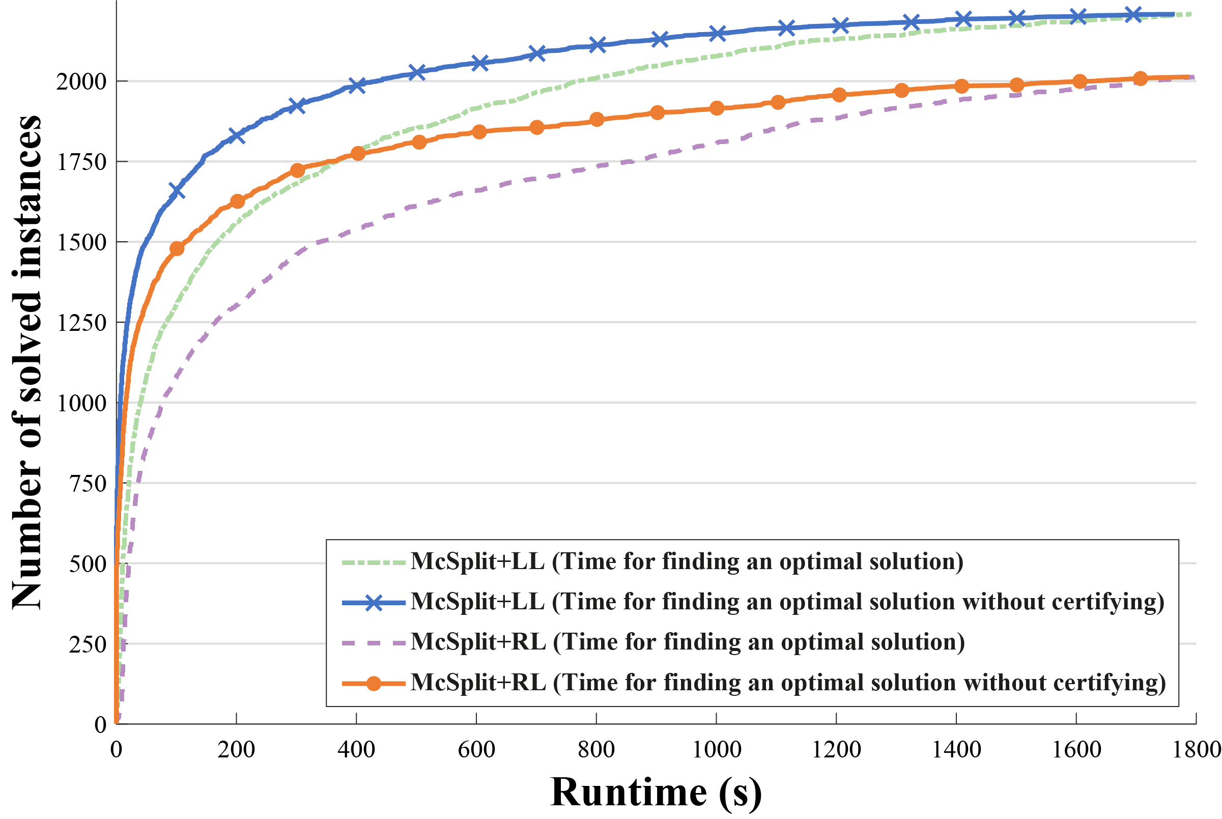
Figure 3: Cactus plots of McSplit+RL and McSplit+LL on the 2,309 moderate MCS instances, which solve 2,013 and 2,208 out of the instances respectively.

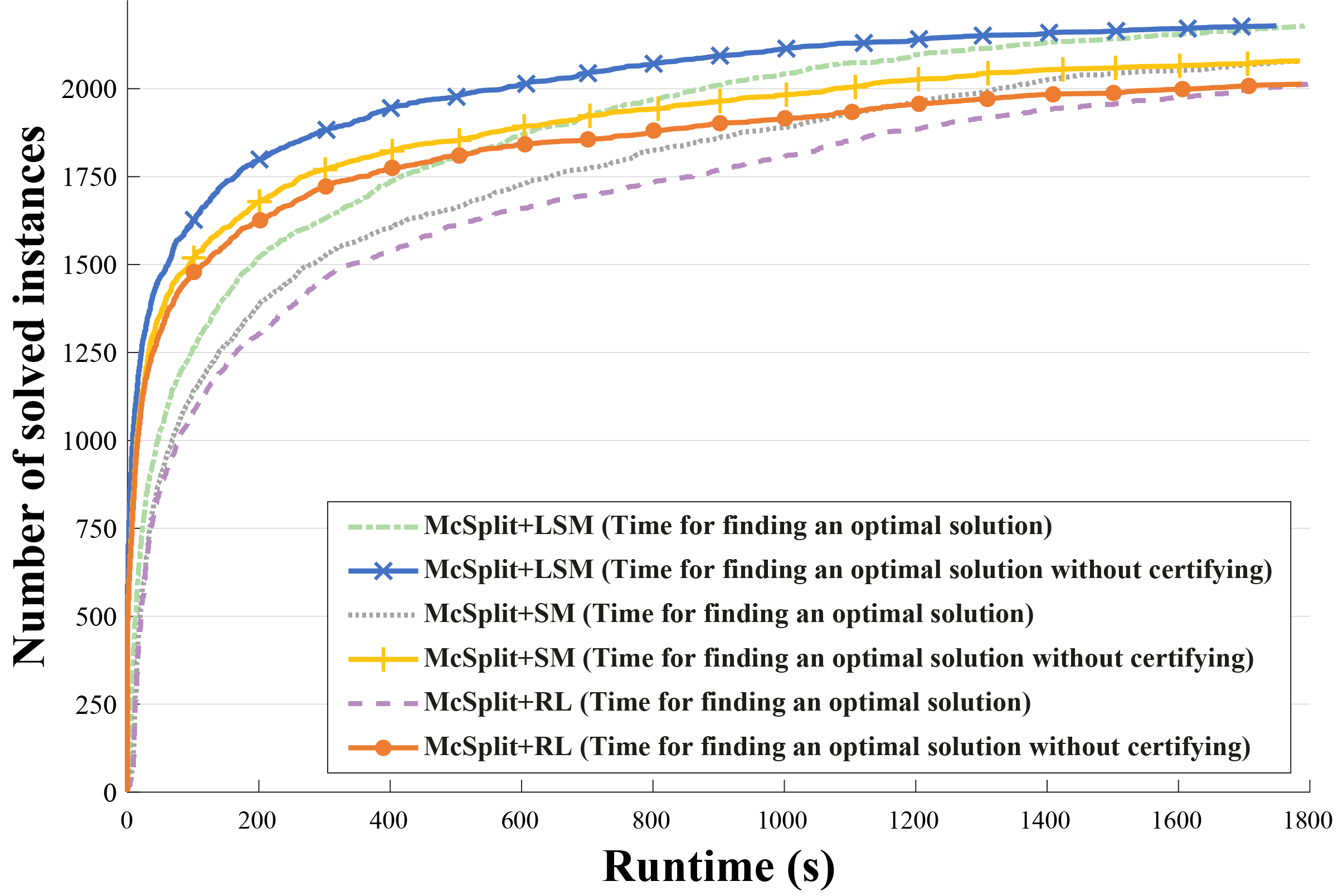
Figure 5: Cactus plots of McSplit+RL, McSplit+SM and McSplit+LSM on the 2,309 moderate MCS instances, which solve 2,013, 2,079 and 2,179 out of the instances respectively.

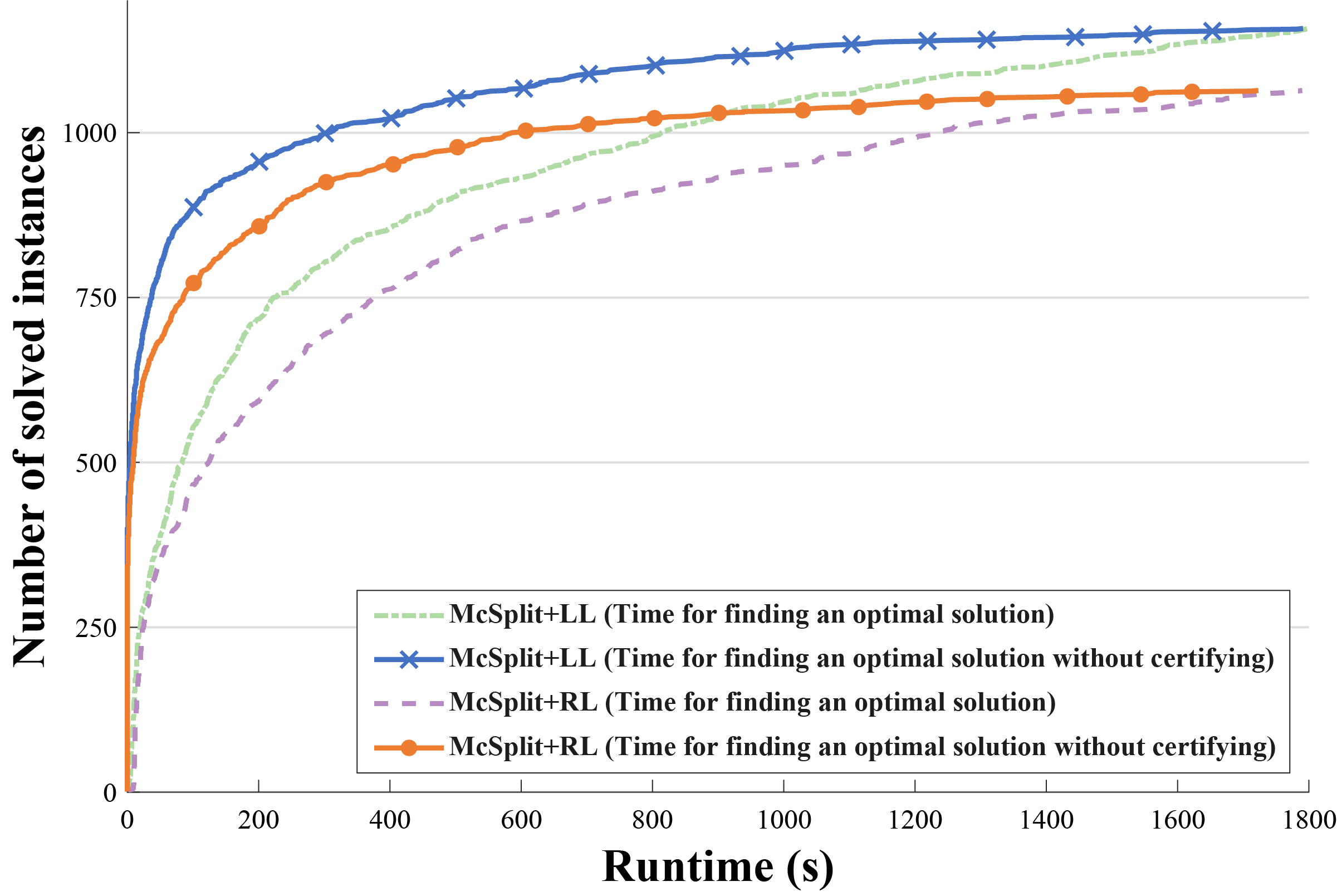
Figure 4: Cactus plots of McSplit+RL and McSplit+LL on the 1,166 moderate MCCS instances, which solve 1,064 and 1,158 out of the instances respectively.

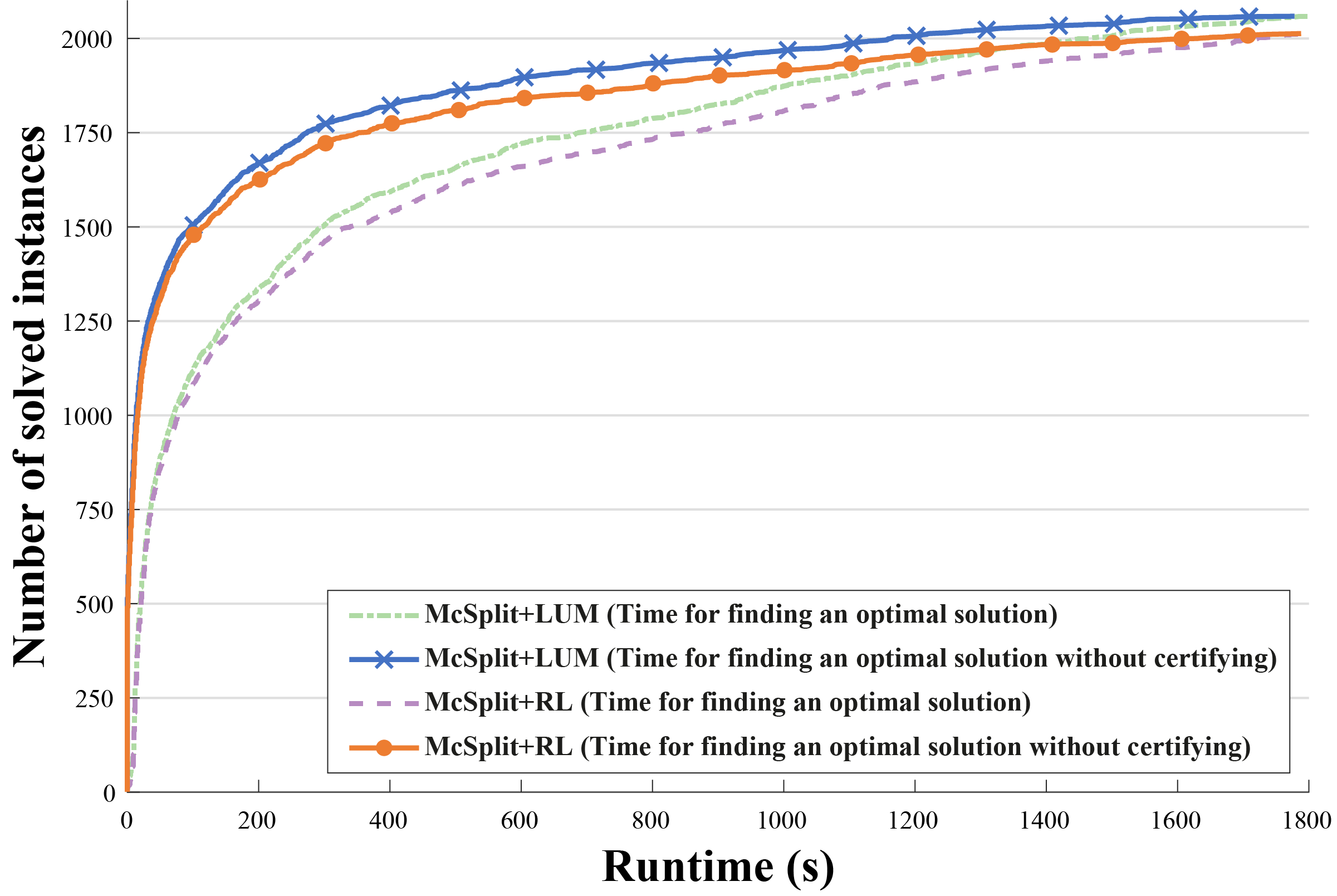
Figure 6: Cactus plots of McSplit+RL and McSplit+LUM on the 2,309 moderate MCS instances, which solve 2,013 and 2,059 out of the instances respectively.

5.2 Benchmark Datasets

The benchmark datasets include 25,552 instances that are divided into several compositions:

• Biochemical reaction Gay et al. (2014) includes 136 directed bipartite graphs (with vertices between 9 and 386), and describe biochemical reaction networks originated from the biomodels.net. It provides 9,180 instances obtained by pairing each of the graphs.

• Images-PR15 Solnon et al. (2015) includes a target graph (with 4,838 vertices) and 24 pattern graphs (with vertices between 4 and 170), which are generated from segmented images. It provides 24 instances.

• Images-CVIU11 Damiand et al. (2011) includes 43 pattern graphs (with vertices between 22 and 151), and 146 target graphs (with vertices between 1,072 and 5,972), which are generated from segmented images. It provides 6,278 instances.

• Meshes-CVIU11 Damiand et al. (2011) includes 6 pattern graphs (with vertices between 40 and 199), and 503 target graphs (with vertices between 208 and 5,873), which are generated from meshes modelling 3D objects. It provides 3,018 instances.

• Scalefree Zampelli et al. (2010); Solnon (2010) includes 100 instances. Each instance is composed of a target graph (with vertices between 200 and 1,000) and a pattern graph (contains 90% of the vertices of the target graph). These instances are randomly generated from scale-free networks.

• Si Zampelli et al. (2010); Solnon (2010) includes 1,170 instances. Each instance is composed of a target graph (with vertices between 200 and 1,296) and a pattern graph (with vertices between 20% and 60% of the target graph). Among these instances, there are bounded valence graphs and modified bounded valence graphs, 4D meshes, and randomly generated graphs.

• LV McCreesh et al. (2017) includes 49 pattern graphs and 48 target graphs (with vertices both between 10 and 128). It provides 2,352 instances.

• LargerLV McCreesh et al. (2017) includes 49 pattern graphs (with vertices between 10 and 128) and 70 target graphs (with vertices between 138 and 6,671). It provides 3,430 instances.

5.3 Comparisons on MCS

The McSplit algorithm is efficient enough and there are lots of small scale instances in the benchmark datasets that can be solved in several seconds. The results on these small scale instances cannot really show the gap of differences on the algorithm efficiency. Hence, we group the 7,226 small scale instances which could be solved by all the tested algorithms within 10 seconds into the easy set, and only provide the average solving time. We also exclude another set of tough instances that cannot be solved by any algorithm within the time limit. Thereafter, we have 2,309 remaining instances that can be solved by at least one of the tested MCS algorithms within the time limit. We denote these medium hard instances as the moderate instances, and will use them for detailed performance comparison.

We compare McSplit+RL with McSplit+LL as illustrated in Figure 3. Each point ($t$, $n$) in a curve of Figure 3 indicates the algorithm solves (finds the optimal solution, with or without certifying) $n$ instances in $t$ seconds, the same in Figures 4, Figure 5, and Figure 6. McSplit+RL solves 2,013 moderate instances while McSplit+LL could solve 2,208 moderate instances. Besides, the average runtimes of McSplit+RL and McSplit+LL on the easy set of instances are 0.83s and 0.51s, respectively. In other words, McSplit+LL solves 9.69% more moderate instances than McSplit+RL, and McSplit+LL is also faster than McSplit+RL in solving the easy instances. The results demonstrate that McSplit+LL outperforms McSplit+RL significantly on the MCS problem.

5.4 Comparisons on MCCS

We also apply our McSplit+LL algorithm to solve the MCCS problem. As the basic version of McSplit does not support solving MCCS on the directed graph, we exclude the directed graph instances (9,180 Biochemical reaction instances) from the datasets.

Using the same datasets processing as in MCS, we first exclude the 2,110 easy instances and the tough instances, and use the remaining 1,166 moderate instances as benchmarks for detailed comparison. The results are illustrated in Figure 4. McSplit+RL solves 1,064 moderate instances, while McSplit+LL solves 1,158 moderate instances (8.83% more than McSplit+RL). Also, the average runtimes of McSplit+RL and McSplit+LL on the easy instances are 2.03s and 1.36s, respectively. The results demonstrate that McSplit+LL also outperforms McSplit+RL significantly on the MCCS problem.

5.5 Ablation Study

In this subsection, we do ablation studies to analyze the effectiveness of the two proposed operators, LSM and LUM.

We first compare three algorithms, McSplit+RL, McSplit+SM and McSplit+LSM, on the MCS instances and the results are illustrated in Figure 5. McSplit+SM is a variant of McSplit+RL that applies our decaying operation on the score lists $S_{0}(\cdot)$ and $S_{1}(\cdot)$ with the short-term threshold value $T_{s}$, called Short Memory (SM). McSplit+LSM is a variant that applies LSM on the top of McSplit.

McSplit+SM solves 2,079 moderate instances and McSplit+LSM solves 2,179 moderate instances which are 3.28% and 8.25% more than McSplit+RL. Besides, the average runtimes of McSplit+SM and McSplit+LSM on the easy instances are 0.82s and 0.53s, respectively. The results show that McSplit+RL can be improved by applying our proposed decaying mechanism, and using LSM instead of SM yields better performance.

Then, we analyze the effectiveness of LUM. We implement it on top of McSplit+RL and obtain a variant algorithm called McSplit+LUM. We compare McSplit+LUM with McSplit+RL on the MCS instances and the results are illustrated in Figure 6. It solves 2,059 moderate instances which is 2.29% better than McSplit+RL. Besides, the average runtime of McSplit+LUM on the easy set of instances was 0.81s.

The ablation studies for both McSplit+LSM and McSplit+LUM demonstrate that our proposed operators could improve the performance and efficiency of the BnB algorithm for both MCS and MCCS problems.

6 Conclusion

In this work, we address the Maximum Common induced Subgraph (MCS) and Maximum Common Connected induced Subgraph (MCCS) problems, and we propose an effective Branch-and-Bound (BnB) algorithm called McSplit+LL for these two problems. McSplit+LL incorporates two proposed operators into the effective BnB algorithm McSplit. The first one is a new branching operator on the BnB algorithm called Long-Short Memory (LSM). LSM finds the different properties of scoring each vertex and each vertex pair, and applies a reasonable policy to make the score of each vertex focus on the short-term reward and the score of each vertex pair focus on the long-term reward. The second one is a general operator called Leaf vertex Union Match (LUM) for MCS and MCCS. LUM allows the common subgraph match multiple leaf pairs whenever a vertex pair is matched, so as to speed up the overall matching at the same time not affect the solution optimality. Both LSM and LUM can improve the efficiency of the BnB algorithm. Besides, LUM is a general vertex-vertex mapping method and could be applied to other graph matching problems.

We do extensive experiments on public instances to evaluate the performance of our proposed algorithm McSplit+LL, and the effectiveness of the two proposed operators LSM and LUM. The results show that McSplit+LL significantly outperforms the best-performing algorithm McSplit+RL for both MCS and MCCS, and both LSM and LUM can improve the efficiency and performance of the BnB algorithm.

References

- Bahiense et al. [2012] Laura Bahiense, Gordana Manić, Breno Piva, and Cid C De Souza. The maximum common edge subgraph problem: A polyhedral investigation. Discrete Applied Mathematics, 160(18):2523–2541, 2012.
- Bai et al. [2021] Yunsheng Bai, Derek Xu, Yizhou Sun, and Wei Wang. Glsearch: Maximum common subgraph detection via learning to search. In The 38th International Conference on Machine Learning, ICML 2021, pages 588–598, 2021.
- Blindell et al. [2015] Gabriel Hjort Blindell, Roberto Castañeda Lozano, Mats Carlsson, and Christian Schulte. Modeling universal instruction selection. In Principles and Practice of Constraint Programming - 21st International Conference, CP 2015, pages 609–626, 2015.
- Bonnici et al. [2013] Vincenzo Bonnici, Rosalba Giugno, Alfredo Pulvirenti, Dennis Shasha, and Alfredo Ferro. A subgraph isomorphism algorithm and its application to biochemical data. BMC bioinformatics, 14(7):1–13, 2013.
- Bruschi et al. [2006] Danilo Bruschi, Lorenzo Martignoni, and Mattia Monga. Detecting self-mutating malware using control-flow graph matching. In Detection of Intrusions and Malware & Vulnerability Assessment, Third International Conference, DIMVA 2006, pages 129–143, 2006.
- Choi et al. [2012] Jaeun Choi, Yourim Yoon, and Byung-Ro Moon. An efficient genetic algorithm for subgraph isomorphism. In Proceedings of the 14th annual conference on Genetic and evolutionary computation, pages 361–368, 2012.
- Damiand et al. [2011] Guillaume Damiand, Christine Solnon, Colin De la Higuera, Jean-Christophe Janodet, and Émilie Samuel. Polynomial algorithms for subisomorphism of nd open combinatorial maps. Computer Vision and Image Understanding, 115(7):996–1010, 2011.
- Duesbury et al. [2017] Edmund Duesbury, John D Holliday, and Peter Willett. Maximum common subgraph isomorphism algorithms. MATCH Communications in Mathematical and in Computer Chemistry, 77(2):213–232, 2017.
- Ehrlich and Rarey [2011] Hans-Christian Ehrlich and Matthias Rarey. Maximum common subgraph isomorphism algorithms and their applications in molecular science: a review. Wiley Interdisciplinary Reviews: Computational Molecular Science, 1(1):68–79, 2011.
- Englert and Kovács [2015] Péter Englert and Péter Kovács. Efficient heuristics for maximum common substructure search. Journal of chemical information and modeling, 55(5):941–955, 2015.
- Gay et al. [2014] Steven Gay, François Fages, Thierry Martinez, Sylvain Soliman, and Christine Solnon. On the subgraph epimorphism problem. Discrete Applied Mathematics, 162:214–228, 2014.
- Giugno et al. [2013] Rosalba Giugno, Vincenzo Bonnici, Nicola Bombieri, Alfredo Pulvirenti, Alfredo Ferro, and Dennis Shasha. Grapes: A software for parallel searching on biological graphs targeting multi-core architectures. PloS one, 8(10):e76911, 2013.
- Hati et al. [2016] Avik Hati, Subhasis Chaudhuri, and Rajbabu Velmurugan. Image co-segmentation using maximum common subgraph matching and region co-growing. In Computer Vision - ECCV 2016 - 14th European Conference, pages 736–752, 2016.
- Jiang and Ngo [2003] Hui Jiang and Chong-Wah Ngo. Image mining using inexact maximal common subgraph of multiple args. In International conference on visual information system, volume 2, page 3, 2003.
- Liu et al. [2020] Yanli Liu, Chu-Min Li, Hua Jiang, and Kun He. A learning based branch and bound for maximum common subgraph related problems. In Proceedings of the AAAI Conference on Artificial Intelligence, volume 34, pages 2392–2399, 2020.
- McCreesh et al. [2017] Ciaran McCreesh, Patrick Prosser, and James Trimble. A partitioning algorithm for maximum common subgraph problems. In The Twenty-Sixth International Joint Conference on Artificial Intelligence, IJCAI 2017, pages 712–719, 2017.
- Park et al. [2013] Younghee Park, Douglas S Reeves, and Mark Stamp. Deriving common malware behavior through graph clustering. Computers & Security, 39:419–430, 2013.
- Raymond and Willett [2002] John W Raymond and Peter Willett. Maximum common subgraph isomorphism algorithms for the matching of chemical structures. Journal of computer-aided molecular design, 16(7):521–533, 2002.
- Sevegnani and Calder [2015] Michele Sevegnani and Muffy Calder. Bigraphs with sharing. Theoretical Computer Science, 577:43–73, 2015.
- Shearer et al. [2001] Kim Shearer, Horst Bunke, and Svetha Venkatesh. Video indexing and similarity retrieval by largest common subgraph detection using decision trees. Pattern Recognition, 34(5):1075–1091, 2001.
- Solnon et al. [2015] Christine Solnon, Guillaume Damiand, Colin De La Higuera, and Jean-Christophe Janodet. On the complexity of submap isomorphism and maximum common submap problems. Pattern Recognition, 48(2):302–316, 2015.
- Solnon [2010] Christine Solnon. Alldifferent-based filtering for subgraph isomorphism. Artificial Intelligence, 174(12-13):850–864, 2010.
- Zampelli et al. [2010] Stéphane Zampelli, Yves Deville, and Christine Solnon. Solving subgraph isomorphism problems with constraint programming. Constraints, 15(3):327–353, 2010.
- Zanfir and Sminchisescu [2018] Andrei Zanfir and Cristian Sminchisescu. Deep learning of graph matching. In 2018 IEEE Conference on Computer Vision and Pattern Recognition, CVPR 2018, pages 2684–2693, 2018.