Detecting Entanglement Between Modes of Light

Abstract

We consider a subgroup of unitary transformations on a mode of light induced by a Mach-Zehnder Interferometer and an algebra of observables describing a photon-number detector proceeded by an interferometer. We explore the uncertainty principles between such observables and their usefulness in performing a Bell-like experiment to show a violation of the CHSH inequality, under physical assumption that the detector distinguishes only zero from non-zero number of photons. We show which local settings of the interferometers lead to a maximal violation of the CHSH inequality.

I Introduction

Multiphoton entangled states Caspani et al. (2017); Dell’Anno et al. (2006) have applications in the fields of quantum communications Qin et al. (2014), computation Langford et al. (2011); Walther et al. (2005) and metrology Paulisch et al. (2019); Afek et al. (2010). Aside from polarisation, optical modes of photons are also another property that can be entangled, as seen for Dicke superradiant photons Paulisch et al. (2019). Such quantum states consist of many photons that may be mode-entangled.

Hilbert space of $n$ photons, which can be in two modes (of polarisation or wave vector), is a symmetric subspace (due to bosonic nature of photons) of $(\mathds{C}^{2})^{\otimes n}$. If the number of photons in experiment is not known, then we deal with direct sum of such spaces with different $n$s (Fock space). On the other hand, we can consider a quantum state of light consisting two modes, each being occupied by an arbitrary number of photons. Such state lives on tensor product of the Hilbert spaces of modes: $\mathcal{H}_{1}\otimes\mathcal{H}_{2}$, and may be entangled in general. Further, if we consider two optical modes, the more natural approach is not to have any restrictions on the number of photons. If the number of photons is fixed, then a state of light is supported in an eigenspace of global photon number: $\hat{N}\otimes\mathds{I}+\mathds{I}\otimes\hat{N}$, being isomorphic to the symmetric sector of $(\mathbb{C}^{2})^{\otimes n}$. The whole Hilbert space $\mathcal{H}_{1}\otimes\mathcal{H}_{2}$ is isomorphic to the whole Fock space. In this paper we will consider entanglement of a quantum state of two modes of light each being occupied by an arbitrary number of photons.

In general, entanglement can be detected by estimating the density matrix of the quantum state of the system White et al. (1999); Schwemmer et al. (2014) and mathematically testing for its non-separability using various separability criteria Horodecki et al. (2009). However, reconstruction of the entire density matrix via quantum state tomography Paris and Rehacek (2004) with many photons in each mode is challenging due to the large number of entries of the density matrix, each requiring many measurements to obtain a desired accuracy. Another approach is to measure an expected value of appropriately chosen entanglement witness Chruściński and Sarbicki (2014) and estimate only one parameter instead of all entries of density matrix.

Bell inequality Bell (1964); Maccone (2013) is an algebraic expression built from local observables satisfying certain assumptions. Expected value of such expression satisfies a certain bound for all separable states. Fixing these observables one obtains an entanglement witness Hyllus et al. (2005).

The most famous Bell inequality is the CHSH inequality Clauser et al. (1969): $\mathds{E}(A_{1}\otimes B_{1}+A_{1}\otimes B_{2}+A_{2}\otimes B_{1}-A_{2}\otimes B_{2})\leq 2$. With appropriate choice of local observables, the CHSH inequality can be violated for certain entangled states with its LHS reaching the value of $2\sqrt{2}$ known as Tsirelson’s bound Cirel’son (1980).

In section II, we consider an action on one mode state of light of a Mach-Zehnder Interferometer (MZI) fed with strong coherent state of light on its second input port. We show, than in the limit of strong coherent field the MZI setup acts as a unitary operation on an input state and hence a projective measure of its output corresponds to a projective measurement on its input. However, for finite coherent fields the action of MZI setup is rather that of a quantum channel and the resulting measurement on its input will be a POVM. In section III, we discuss how in this limit the quantum channel becomes a unitary transformation and the POVM becomes a projective measurement. We will proceed in the limiting scenario when the MZI realises a unitary transformation.

Next, in section IV, we discuss the unitary operators related to the action of MZI and the algebra of observables representing photon number measurements proceeded by an interferometer. In particular, we discuss uncertainty relations between these observables.

Finally, in section V we discuss, how one can perform a Bell-like experiment measuring the violation of CHSH inequality in such a scenario. We show that, with appropriate setups of interferometers, we are able to obtain the maximum possible violation of CHSH inequality.

II Unitary Transformations

For photons, optical components such as beam splitters and phase shifters can be used to generate unitary transformations in the cumulative Fock state.

II.1 Beam Splitter Implementation

The effect of a beam splitter on a photonic state can be envisioned as a unitary operation on the incoming photon states. A typical ”quantum” beam splitter schematic is shown in Fig. 1. The photon annihilation operators at the output ports [$\hat{a}_{2}$, $\hat{a}_{3}$] corresponding to the respective input ports [$\hat{a}_{0}$, $\hat{a}_{1}$] are transformed as Windhager et al. (2011):

Figure 1: Quantum Beam Splitter. Schematic diagram of a quantum beam splitter with two input ports ($\hat{a}_{0}$, $\hat{a}_{1}$) and two output ports ($\hat{a}_{2}$, $\hat{a}_{3}$), with corresponding reflectivities and transmittivities, ($r$, $t$) and ($r^{\prime}$, $t^{\prime}$) at the input and output ports, respectively.

$$\begin{pmatrix}\hat{a}_{2}\\ \hat{a}_{3}\end{pmatrix}=\begin{pmatrix}t^{\prime}&r\\ r^{\prime}&t\end{pmatrix}\begin{pmatrix}\hat{a}_{0}\\ \hat{a}_{1}\end{pmatrix}$$ (1)

where ($r$, $t$)[($r^{\prime}$, $t^{\prime}$)] are the reflectance and transmittance of the beam splitter at the input[output] ports, respectively. Due to energy conservation, these numbers are complex in general and form a unitary matrix, i.e:

$$|t|^{2}+|r|^{2}=1$$ (2)

$$|t^{\prime}|^{2}+|r^{\prime}|^{2}=1$$ (3)

$$t^{\prime}r^{*}+r^{\prime}t^{*}=0$$ (4)

It implies in particular, that $|t|=|t^{\prime}|$ and $|r|=|r^{\prime}|$. The above equations are often referred to as Stokes’ laws. In general, for a single photon input, the beam splitter performs a rotation on the Poincare sphere Leonhardt (2003).

Consider a general many-photon Fock state:

$$\ket{\psi}=\sum_{n=0}^{\infty}c_{n}\ket{n}=\sum_{n=0}^{\infty}c_{n}\frac{1}{\sqrt{n!}}(\hat{a}_{0}^{\dagger})^{n}\ket{0}$$ (5)

and a coherent state of light $\hat{D}_{1}(\alpha)\ket{0}_{1}$, where

$$\hat{D}_{1}(\alpha)=\mathrm{exp}(\alpha\hat{a}^{\dagger}_{1}-\alpha^{*}\hat{a}_{1})$$ (6)

is the displacement operator, to be incident on the first and second port of the beam splitter, respectively. The total input state of the BS is

$$\ket{\psi}_{0}\otimes\ket{\alpha}_{1}=\sum_{n=0}^{\infty}c_{n}\frac{1}{\sqrt{n!}}(\hat{a}_{0}^{\dagger})^{n}\ket{0}_{0}\otimes\hat{D}_{1}(\alpha)\ket{0}_{1}$$ (7)

Assuming the beam splitter operator to be $\hat{U}_{1}$ from (1), we get the photon annihilation operators ($\hat{a}_{0}$ and $\hat{a}_{1}$) in terms of that at the output ports ($\hat{a}_{2}$ and $\hat{a}_{3}$) as,

$$\begin{gathered}\hat{a}_{0}=t^{\prime*}\hat{a}_{2}+r^{\prime*}\hat{a}_{3}\quad\textrm{and}\quad\hat{a}_{1}=r^{*}\hat{a}_{2}+t^{*}\hat{a}_{3}\end{gathered}$$ (8)

where we have used the Stokes’ laws: $r^{*}t^{\prime}+r^{\prime}t^{*}=0$ and $\absolutevalue{r}^{2}+\absolutevalue{t}^{2}=1$ along with [Eq. 1].

Applying the beam splitter (BS) transformation (1) to operators in the input state formula (7) we obtain

$$\begin{gathered}\ket{\psi}_{0}\otimes\ket{\alpha}_{1}\xrightarrow[]{BS}\ket{\Psi}_{out}=\mathrm{exp}(\alpha(r\hat{a}_{2}^{\dagger}+t\hat{a}_{3}^{\dagger})-\alpha^{*}(r^{*}\hat{a}_{2}+t^{*}\hat{a}_{3}))\sum_{n=0}^{\infty}\frac{c_{n}}{\sqrt{n!}}(t^{\prime}\hat{a}_{2}^{\dagger}+r^{\prime}\hat{a}_{3}^{\dagger})^{n}\ket{0}_{2}\otimes\ket{0}_{3}\\ =\mathrm{exp}(r\alpha\hat{a}_{2}^{\dagger}-r^{*}\alpha^{*}\hat{a}_{2})\mathrm{exp}(t\alpha\hat{a}_{3}^{\dagger}-t^{*}\alpha^{*}\hat{a}_{3})\sum_{n=0}^{\infty}c_{n}\frac{1}{\sqrt{n!}}(t^{\prime}\hat{a}_{2}^{\dagger}+r^{\prime}\hat{a}_{3}^{\dagger})^{n}\ket{0}_{2}\otimes\ket{0}_{3}\\ =\hat{D}_{2}(r\alpha)\hat{D}_{3}(t\alpha)\sum_{n=0}^{\infty}c_{n}\frac{1}{\sqrt{n!}}(A^{\dagger})^{n}\ket{0}_{2}\otimes\ket{0}_{3}\end{gathered}$$ (9)

where $A^{\dagger}=t^{\prime}\hat{a}_{2}^{\dagger}+r^{\prime}\hat{a}_{3}^{\dagger}$. In the limit of a highly reflective beam splitter and a highly intense coherent state:

$$r\xrightarrow[]{}1,\quad t\alpha=\mathrm{const.}$$ (10)

the output state formula (9) reduces to:

$$\ket{\Psi}_{out}=\ket{r\alpha}_{2}\otimes\hat{D}_{3}(t\alpha)\ket{\psi}_{3}$$ (11)

Thus, we achieve the incoming coherent state with reduced intensity ($\ket{r\alpha}_{2}$) and the incoming photonic state displaced by $t\alpha$ at the output ports 2 and 3 respectively. Using these results whereby the beam splitter displaces any quantum state, one can physically implement unitary transformations over the photonic wavepacket. However in this case, the parameters of displacement, i.e., $t$ and $\alpha$ depend only on the transmittivity of the beam splitter and the input coherent field intensity, respectively. Moreover, a highly reflective beam splitter with $r\xrightarrow[]{}1$ is practically difficult to construct. To eliminate such problems with the implementation of the scheme and to exercise further degree of tunability on the displacement operator, we describe the case of using a MZI setup with the same input state (see [Eq. 7]).

II.2 Mach-Zehnder Interferometric Implementation

Figure 2: Mach-Zehnder Interferometer. MZI setup with a phase shift ($\phi$) in one of the arms of the interferometer. Two 50:50 beam splitters (BS₁ and BS₂, with BS₂ $180^{o}$ rotated w.r.t BS₁), i.e., having equal magnitudes of reflectivity and transmittivity, are used along with two mirrors (M₁ and M₂) for such an interferometer.

A MZI can be approximated as a four-port device Yurke et al. (1986) as shown in Fig. 2. The composite optical elements of the MZI setup each correspond to a unitary operation over the field states. Defining the matrix associated to the effect of the phase shifter over the input state as,

$$P_{\phi}=\begin{pmatrix}1&0\\ 0&e^{i\phi}\end{pmatrix}$$ (12)

Using the definition of the beam splitter operator from [Eq. 1], we find the transformation of the annihilation operators to be,

$$\begin{gathered}\begin{pmatrix}\hat{a}_{4}\\ \hat{a}_{5}\end{pmatrix}=\begin{pmatrix}t_{2}^{\prime}&r_{2}\\ r_{2}^{\prime}&t_{2}\end{pmatrix}\begin{pmatrix}1&0\\ 0&e^{i\phi}\end{pmatrix}\begin{pmatrix}t_{1}^{\prime}&r_{1}\\ r_{1}^{\prime}&t_{1}\end{pmatrix}\begin{pmatrix}\hat{a}_{0}\\ \hat{a}_{1}\end{pmatrix}\\ \end{gathered}$$

Now, assuming that two identical beam splitters are arranged in the MZI setting such that the first beam splitter is aligned in the reverse direction relative to the second as shown in Fig. 2, we have,

$$\begin{gathered}\begin{pmatrix}\hat{a}_{4}\\ \hat{a}_{5}\end{pmatrix}=\begin{pmatrix}t^{\prime}&r\\ r^{\prime}&t\end{pmatrix}\begin{pmatrix}1&0\\ 0&e^{i\phi}\end{pmatrix}\begin{pmatrix}t^{\prime*}&r^{*}\\ r^{\prime*}&t^{*}\end{pmatrix}\begin{pmatrix}\hat{a}_{0}\\ \hat{a}_{1}\end{pmatrix}\\ =\begin{pmatrix}\absolutevalue{t^{\prime}}^{2}+\absolutevalue{r}^{2}e^{i\phi}&r^{\prime*}t^{\prime}(1-e^{i\phi})\\ r^{\prime}t^{\prime*}(1-e^{i\phi})&\absolutevalue{r^{\prime}}^{2}+\absolutevalue{t}^{2}e^{i\phi}\end{pmatrix}\begin{pmatrix}\hat{a}_{0}\\ \hat{a}_{1}\end{pmatrix},\end{gathered}$$

using [Eq. 4]. Now, assume both to be 50:50 beam splitters, i.e., $\absolutevalue{t}=\absolutevalue{t^{\prime}}=\absolutevalue{r}=\absolutevalue{r^{\prime}}=\frac{1}{\sqrt{2}}$. Also since all coefficients of reflection and transmission are complex numbers we can write, $r^{\prime}=\absolutevalue{r^{\prime}}e^{i\gamma_{1}}$ and $t^{\prime}=\absolutevalue{t^{\prime}}e^{i\gamma_{2}}$. Therefore, the above equation reduces to:

$$\begin{pmatrix}\hat{a}_{4}\\ \hat{a}_{5}\end{pmatrix}=\frac{1}{2}\begin{pmatrix}1+e^{i\phi}&e^{i\gamma}(1-e^{i\phi})\\ e^{-i\gamma}(1-e^{i\phi})&1+e^{i\phi}\end{pmatrix}\begin{pmatrix}\hat{a}_{0}\\ \hat{a}_{1}\end{pmatrix}\\$$ (13)

where $\gamma=\gamma_{2}-\gamma_{1}$. Alternating roles of $\hat{a}_{4}$ and $\hat{a}_{5}$ one gets:

$$\begin{pmatrix}\hat{a}_{5}\\ \hat{a}_{4}\end{pmatrix}=\begin{pmatrix}T^{\prime}&R\\ R^{\prime}&T\end{pmatrix}\begin{pmatrix}\hat{a}_{0}\\ \hat{a}_{1}\end{pmatrix},\\$$ (14)

where:

$$\begin{gathered}R=R^{\prime}=\frac{1+e^{i\phi}}{2},\\ T=\frac{e^{i\gamma}(1-e^{i\phi})}{2},\\ T^{\prime}=\frac{e^{-i\gamma}(1-e^{i\phi})}{2}.\end{gathered}$$ (15)

Thus the MZI scattering matrix is equivalent to that of a beam spitter with tunable parameters, namely, effective reflectivities ($R$ and $R^{\prime}$)s and transmitivities ($T$ and $T^{\prime}$).

In the limit $\phi\xrightarrow[]{}0$, we can use the Taylor expansion of $e^{i\phi}$ up to second term such that $1-e^{i\phi}\simeq-i\phi$. So [Eqs. 15] modify to,

$$\lim_{\phi\to 0}R=\lim_{\phi\to 0}\frac{2+i\phi}{2}\simeq 1$$ (16)

$$\lim_{\phi\to 0}T=\lim_{\phi\to 0}-\frac{i\phi}{2}e^{i\gamma}\simeq 0$$ (17)

Drawing an analogy to Sec. II.1, we would require $T\alpha$ to remain constant (see [Eq. 10]). For this: $|\alpha|\sim 1/\phi$. Proportionality constant and phase of $\alpha$ will establish a proper displacement in [Eq. 11]. We are able to displace the input quantum state by $T\alpha$ using a MZI setup with two identical 50:50 beam splitters and small phase difference between arms, fed with strong laser field in a coherent state.

In case of $\alpha$ being finite, the state of the outputs is weakly entangled and tends to a separable state when $\alpha\to\infty$.

III POVMs

Let us assume from now, that the bottom arm of the MZI setup is ended by a photon number detector i.e. we measure intensity of field represented by the photon number operator $\hat{N}=\hat{a}^{\dagger}\hat{a}$. The MZI setup applies a global unitary transformation on the product state of the composite system (coherent state + multiphoton state). Let the projectors on the coherent and multiphoton states be $\sigma=\outerproduct{\alpha}{\alpha}$ and $\rho=\outerproduct{\psi}{\psi}$, respectively.

Thus, the state of the outputs of the MZI setup fed with an input state $\sigma\otimes\rho$ is,

$$\mathrm{\varepsilon}=\mathrm{U}(\sigma\otimes\rho)\mathrm{U}^{\dagger}$$ (18)

where $\mathrm{U}$ is the unitary operation performed by the MZI setup. Note that $\mathrm{U}$ has infinite dimensionality in the Schrödinger picture. The blocks of matrix $\mathrm{\varepsilon}$ are:

$$\mathrm{\varepsilon_{mn}}=\mathrm{Tr_{1}}(\varepsilon\outerproduct{m}{n}\otimes\mathds{I})=\sum_{ij}\mathrm{U_{mi}}(\sigma_{ij}\rho)(\mathrm{U_{nj}})^{\dagger}$$ (19)

where $\mathrm{U_{mi}}$ is the $mi$-th block of $U$.

In the standard Fock basis, $\sigma_{ij}=\innerproduct{i}{\alpha}\innerproduct{\alpha}{j}\equiv\alpha_{i}\alpha^{*}_{j}$. Substituting the same in [Eq. 19] and evaluating the trace of this quantum operation w.r.t the first subsystem ($\sigma$) we obtain:

$$\mathrm{\varepsilon} =\sum_{k}\sum_{ij}(\alpha_{i}\mathrm{U_{ki}})\rho(\alpha_{j}\mathrm{U_{kj}})^{\dagger}=\sum_{k}E\rho E_{k}^{\dagger}$$ (20)

where $E_{k}=\sum_{i}\alpha_{i}\mathrm{U}_{ki}$ act as Kraus operators. It can be easily checked that these operators satisfy the completeness relation $\sum_{k}E_{k}E_{k}^{\dagger}=\mathds{I}$ (trace preservation).

The probability of observing $i$ photons at the detector is,

$$p(i) =Tr(\outerproduct{i}{i}\sum_{k}(\sum_{j}\alpha_{j}\mathrm{U_{kj}})\rho(\sum_{j}\alpha_{j}\mathrm{U_{kj}})^{\dagger}))$$

$$\equiv Tr(M_{i}\rho)$$ (21)

where $M_{i}=\sum_{k}(\alpha_{j}\mathrm{U_{kj}})^{\dagger}\outerproduct{i}{i}(\alpha_{j}\mathrm{U_{kj}})$ is the effect corresponding to measuring $i$ photons at the output. Using [Eq. 9], we derive this effect for the MZI setting to be:

$$M_{i}=e^{-\absolutevalue{T\alpha}^{2}}\frac{|T\alpha|^{2i}}{i!}\sum_{n,n^{\prime}=0}^{\infty} (-R^{\prime*}T\alpha)^{n^{\prime}}(-R^{\prime*}T\alpha)^{*n}\sum_{k=0}^{\min\{n,n^{\prime}\}}\frac{|R^{\prime}\alpha|^{-2k}}{k!}\frac{\sqrt{n^{\prime}!n!}}{(n^{\prime}-k)!(n-k)!}$$

$$\sum_{j=0}^{\min\{i,n^{\prime}-k\}}\frac{i!(n^{\prime}-k)!(-|T\alpha|)^{-2j}}{j!(i-j)!(n^{\prime}-k-j)!}\sum_{j=0}^{\min\{i,n-k\}}\frac{i!(n-k)!(-|T\alpha|)^{-2j}}{j!(i-j)!(n-k-j)!}\outerproduct{n^{\prime}}{n}$$ (22)

In the limit $|R^{\prime}|\to 1,T\alpha=\mathrm{const.}$ [discussed in Sec. II.2], only the summand corresponding to $k=0$ survives in [Eq. III] and $M_{i}$ reduces to a projector onto the state vector $\ket{i,T\alpha}=\hat{D}(T\alpha)\ket{i}$ of a generalised coherent state (GCS):

$$M_{i}\to\hat{D}^{\dagger}(T\alpha)\outerproduct{i}{i}\hat{D}(T\alpha)$$ (23)

and we obtain a projective measurement as the limiting case. (See Appendix A for details).

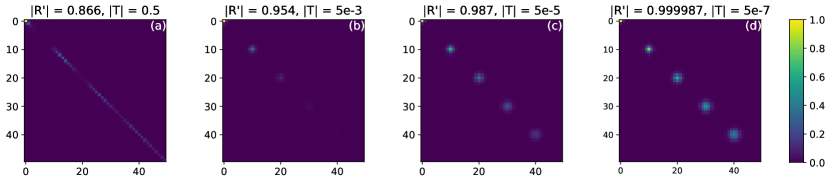
Figure 3: POVM element $M_{i}$: Numerically generated plot for the matrix representation (having dimensions $50\times 50$) of the POVM $|M_{i}|$ for $i=0$ to $50$ in gaps of $10$. The value of $\alpha=0.1/T$ such that $T\alpha$ is kept constant throughout the simulation. The matrix $M_{i}$ is generated for different values of reflectivity ($|R^{\prime}|$) and transmittivity ($|T|$) as shown in the subfigures: (a) $|R^{\prime}|=0.866$, $|T|=0.5$; (b) $|R^{\prime}|=0.954$, $|T|=5\times 10^{-3}$; (c) $|R^{\prime}|=0.987$, $|T|=5\times 10^{-5}$ and (d) $|R^{\prime}|=0.999987$, $|T|=5\times 10^{-7}$.

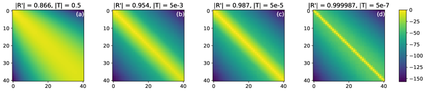
Figure 4: Overlap between $M_{i}$ and $M_{j}$: Numerically generated plot (in logarithmic scale) for the overlap between POVMs $M_{i}$ and $M_{j}$ with $i,j\in[0,40]$. The value of $\alpha=0.1/T$ such that $T\alpha$ is kept constant throughout the simulation. The matrix $M_{i}$ is generated for different values of reflectivity (R’) and transmittivity (T) as shown in the subfigures: (a) $|R^{\prime}|=0.866$, $|T|=0.5$; (b) $|R^{\prime}|=0.954$, $|T|=5\times 10^{-3}$; (c) $|R^{\prime}|=0.987$, $|T|=5\times 10^{-5}$ and (d) $|R^{\prime}|=0.999987$, $|T|=5\times 10^{-7}$.

In Fig. 3 we have shown in one plot the numerically obtained matrix representations of $M_{i}$ ($i\in\{0,10,\dots,40\}$) for different values of $|R^{\prime}|$ and $|T|$ of the MZI setup. From Figs. 3 (a) to (d), the values of $R^{\prime}$ and $T$ slowly approach the limit of $|R^{\prime}|=|R|\xrightarrow[]{}1$, $T\xrightarrow[]{}0$ and $\alpha\xrightarrow[]{}\infty$ under the condition that $T\alpha$ remains constant.

Next we have numerically estimated the overlap $\innerproduct{M_{j}}{M_{i}}_{HS}=Tr(M_{j}^{\dagger}M_{i})$ between the effects of $M_{i}$ and $M_{j}$ for each $i,j\in[0,40]$, estimating the effect’s operators by $52\times 52$ matrices. We gather overlaps into a square matrix, being the (left-upper block of a) Gram matrix of the POVM. We have plotted the absolute values of its entries in the logarithmic scale

[see Figs. 4 (a)-(d)]. We observe that for $|R^{\prime}|=0.999987$ and $|T|=5\times 10^{-7}$, we obtain an almost diagonal matrix, as expected for almost orthonomal operators $M_{i}$ approximating the projective measurement.

IV Maassen-Uffink Uncertainty Principle

In the previous section, we described the POVMs associated with the measurement made by a photon number detector at one arm of the MZI setting. While the MZI setup realizes the displacement operator $\hat{D}(\beta)$ under certain limits [discussed in Sec. II.2 and III], the setup MZI + detector measures the observable $\hat{D}^{\dagger}(\beta)\hat{N}\hat{D}(\beta)$. We would like to comment now on the uncertainty relation between two such observables for two different values of $\beta$.

The Maassen-Uffink uncertainty principle Maassen and Uffink (1988) deals with entropic uncertainties relying on Shannon entropy as a measure of uncertainty. The probability distributions for any quantum state $\ket{\psi}$ w.r.t two observables $A$ and $B$ having sets of eigenvectors ${\ket{a_{j}}}$ and ${\ket{b_{j}}}$ are $p=\absolutevalue{\bra{a_{j}}\ket{\psi}}^{2}$ and $q=\absolutevalue{\bra{b_{j}}\ket{\psi}}^{2}$, respectively. The Shannon entropy corresponding to any general probability distribution $x=(x_{1},...,x_{N})$ is given as $H(x)=-\sum_{j}x_{j}\log_{2}x_{j}$. For an $N$-dimensional Hilbert space, the Maassen-Uffink uncertainty principle is given as,

$$H(p)+H(q)\geq-2\log_{2}c$$ (24)

where $c=\max_{j,k}\absolutevalue{\bra{a_{j}}\ket{b_{k}}}$. The right-hand side of [Eq. 24] is independent of $\ket{\psi}$, i.e., the state of the system. Thus, non-trivial information is gathered about the probability distributions $p$ and $q$ from this relation, provided $c<1$.

In the context of our problem, first we need to estimate the lower bound in [Eq. 24]. The observables $\hat{D}^{\dagger}(\beta_{1})\hat{N}\hat{D}(\beta_{i})$, $i\in\{1,2\}$ has eigenbases $\{D^{\dagger}(\beta_{i})\ket{n}\}$ respectively. We want to find the maximum of $|\bra{m}D(\beta_{1})D^{\dagger}(\beta_{2})\ket{n}|=|\bra{m}D(\beta_{1}-\beta_{2})\ket{n}|$ over $n,m$. Let us provide the notation $\beta=\beta_{1}-\beta_{2}$. The displacement operator $\hat{D}(\beta)$ acting on a state vector $\ket{n}$ produces a state known as a generalised coherent state (GCS) Boiteux and Levelut (1973); Philbin (2014); De Oliveira et al. (1990), which can be decomposed in the occupancy number basis:

$$\ket{n,\beta}=\hat{D}(\beta)\ket{n}=\sum_{k=0}^{\infty}C_{n,k}\ket{k}$$

, where

$$C_{n,k}=e^{-\absolutevalue{\beta}^{2}/2}\sum_{i=0}^{min(n,k)}\frac{\sqrt{n!}(-\beta^{*})^{n-i}}{\sqrt{i!}(n-i)!}\frac{\sqrt{k!}(\beta)^{k-i}}{\sqrt{i!}(k-i)!}$$ (25)

[see Appendix B].

Now, numerically analysing $C_{n,k}$ [Eq. 25] for many values of $\beta$, we have obtained the following observation:

Conjecture 1

The maximum of $|C_{n,k}|$ is realised for $n=0$ (or $k=0$).

[see Fig. 5].

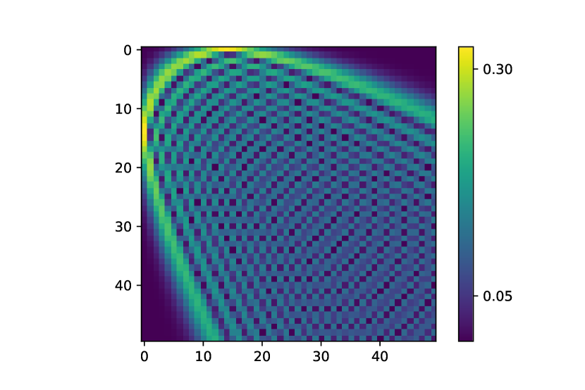
Figure 5: Displacement Operator: Matrix Elements Numerically generated plot for the absolute values of matrix elements ($\absolutevalue{C_{n,k}}=\absolutevalue{\bra{n}\hat{D}(\beta)\ket{k}}$) of the displacement operator ($\hat{D}(\beta)$) with $\beta=3.8$.

Using the above conjecture, we proceed analytically. It is straightforward to observe, that the sequence $C_{0,k}$ (coefficients of a coherent state in the occupancy number basis) satisfies the following recurrence relation: $C_{0,k}=\frac{\beta}{\sqrt{k}}C_{0,k-1}$ and we easily observe, that $\max_{k}|C_{0,k}|$ is at $k=\absolutevalue{\beta}^{2}$ (rounded to one of the nearest integers).

Hence we get,

$$\max_{n,k}|C_{n,k}|=|C_{0,\absolutevalue{\beta}^{2}}|=e^{-\absolutevalue{\beta}^{2}/2}\frac{|\beta|^{\absolutevalue{\beta}^{2}}}{\sqrt{\Gamma(\absolutevalue{\beta}^{2}+1)}}$$ (26)

Applying Stirling’s formula to $\Gamma(\absolutevalue{\beta}^{2}+1)$, i.e., $\Gamma(\absolutevalue{\beta}^{2}+1)>\sqrt{2\pi\absolutevalue{\beta}^{2}}\bigg{(}\frac{\absolutevalue{\beta}^{2}}{e}\bigg{)}^{\absolutevalue{\beta}^{2}}$ we have,

$$\absolutevalue{C_{0,\absolutevalue{\beta}^{2}}}<e^{-\absolutevalue{\beta}^{2}/2}\frac{\absolutevalue{\beta}^{\absolutevalue{\beta}^{2}}}{\bigg{(}\sqrt{2\pi\absolutevalue{\beta}^{2}}\bigg{(}\frac{\absolutevalue{\beta}^{2}}{e}\bigg{)}^{\absolutevalue{\beta}^{2}}\bigg{)}^{1/2}}$$ (27)

On simplifying the above equation, we arrive at,

$$\absolutevalue{C_{0,\absolutevalue{\beta}^{2}}}<\frac{1}{\sqrt[4]{2\pi\absolutevalue{\beta}^{2}}}.$$ (28)

hence $c<\left(2\pi\absolutevalue{\beta}^{2}\right)^{-1/4}$ and the [Eq. 24] gives us:

$$H(p)+H(q)\geq\frac{1}{2}\log_{2}(2\pi\absolutevalue{\beta_{1}-\beta_{2}}^{2})$$ (29)

where $p_{i}=\absolutevalue{\bra{i}\hat{D}(\beta_{1})\ket{\psi}}^{2}$, $q_{i}=\absolutevalue{\bra{i}\hat{D}(\beta_{2})\ket{\psi}}^{2}$ and $\absolutevalue{\beta}=\absolutevalue{\beta_{1}-\beta_{2}}$. In a finite dimensional Hilbert space, the bound in the [Eq. 24] is for a pair of observables having their eigenbases unbiased (related by a Hadamard unitary matrix) and cannot exceed $\log_{2}d$, where $d$ is the dimension of the Hilbert space. In our case the dimension of the Hilbert space is infinite and the bound in [Eq. 29] is unbounded and grows with the moduli of the difference of the displacements.

V CHSH Inequality

The violation of the CHSH inequality is seen as the experimental confirmation of the entangled nature of the concerned states Clauser et al. (1969). Therefore, in this section we theorise the observables for experimentally establishing a test for the entanglement of the multiphoton state ($\ket{\psi}$), described in the previous sections.

Experimental realization of multiphoton entanglement detection would require number-resolved measurements on the outcoming photonic wavepacket from the beam splitter. Till date, the best possible resolution for photon detection is restricted to measuring temporally spaced single photons Hadfield (2009), i.e., identifying the number of photons in a single pulse is not yet possible. Therefore, when a detector is placed at the output port of the MZI setting, either zero or non-zero number of photons will be reported by the detector. Let us prescribe outputs $-1$ and $1$ to these possibilities. The related observable will be:

$$A(\beta) =(-1)\outerproduct{\beta}{\beta}+(+1)(\mathds{I}-\outerproduct{\beta}{\beta})$$

$$=\mathds{I}-2\outerproduct{\beta}{\beta}$$ (30)

Here $\ket{-\beta}=\hat{D}^{\dagger}(\beta)\ket{0}$ is the vector corresponding to the measurement output of $-1$.

Let us assume that we have two such observables $A(\beta_{1})$ and $A(\beta_{2})$. For a state vector $\Psi$, the output statistics of both observables will be determined by two probabilities of getting an output of -1 for each of them:

$$p(A_{i}=-1|\Psi)=|\innerproduct{\Psi}{-\beta_{i}}|^{2},\ i=1,2$$ (31)

The output statistics is determined by the projection of $\Psi$ ($\Pi_{V}\Psi$) onto $V=\mathrm{span}\{\beta_{1},\beta_{2}\}$. While $\Pi_{V}\Psi$ can have arbitrary norm $\leq 1$, the effective Hilbert space must have at least one direction orthogonal to $V$, to project a normalised $\Psi$ onto $\Pi_{V}\Psi$ of desired norm. One orthogonal direction is enough to obtain it and hence the dimension of the effective Hilbert space for both observables is 3.

Let us fix an orthonormal basis of the effective Hilbert space ($\mathcal{H}$). Assuming that the displacement applied is $-\beta_{1}$ or $-\beta_{2}$ let,

$$\ket{e_{1}} =\ket{\beta_{1}},$$

$$\ket{e_{2}} =\frac{\ket{\beta_{2}}-\innerproduct{\beta_{1}}{\beta_{2}}\ket{\beta_{1}}}{\sqrt{1-|\innerproduct{\beta_{1}}{\beta_{2}}|^{2}}}$$

$$=\frac{\ket{\beta_{2}}-\innerproduct{\beta_{1}}{\beta_{2}}\ket{\beta_{1}}}{\sqrt{1-\exp(-|\beta_{1}-\beta_{2}|^{2})}}$$ (32)

and let $\ket{e_{3}}$ be an arbitrary vector orthogonal to $\ket{\beta_{1}}$, $\ket{\beta_{2}}$. Considering $\{\ket{e_{1}},\ket{e_{2}},\ket{e_{3}}\}$ as the basis for $\mathcal{H}$, the observables $A_{1}$, $A_{2}$ are represented by matrices:

$$A(\beta_{1})=\begin{pmatrix}-1&0&0\\ 0&1&0\\ 0&0&1\end{pmatrix}$$ (33)

$$A(\beta_{2})=\begin{pmatrix}1-2E&-2\sqrt{E(1-E)}&0\\ -2\sqrt{E(1-E)}&-1+2E&0\\ 0&0&1\end{pmatrix},$$ (34)

where $E=\exp(-|\beta_{1}-\beta_{2}|^{2})$.

Let us assume that we have a source producing copies of a two-mode, multiphoton state. Consider an experiment, where these two modes become spatially separated and for each state from the pair, simultaneous measurements are performed in two distant laboratories. First laboratory chooses the displacement in the MZI setup to be $-\beta_{1}$ or $-\beta_{2}$ randomly, measuring the observables $A(\beta_{1})$ and $A(\beta_{2})$. Similarly, the second laboratory chooses randomly the displacement in the MZI setup to be $-\beta_{3}$ or $-\beta_{4}$, measuring observables $A(\beta_{3})$ and $A(\beta_{4})$. Both parties then perform a Bell-like experiment, similar to  Bell (1964); Clauser et al. (1969).

Each party possesses a pair of dichotomic observables with outcomes $\pm 1$, hence the celebrated CHSH inequality:

$$|\mathbb{E}\big{(}A(\beta_{1})\otimes A(\beta_{3})+A(\beta_{2})\otimes A(\beta_{3})$$

$$+A(\beta_{1})\otimes A(\beta_{4})-A(\beta_{2})\otimes B(\beta_{4})\big{)}|\leq 2$$

should hold for classically correlated states. The expression on the left-hand side is a non-local observable. Its expected value is reconstructed from local measurements. If the absolute value of its expected value exceeds 2, the state of two modes must be entangled.

The CHSH inequality can be violated if the maximal eigenvalue of the non-local observable it deals with, exceeds 2. The maximum eigenvalue of the observable is equal to:

$$\lambda_{max}=2\sqrt{1+4\sqrt[4]{E_{1}(1-E_{1})}\sqrt[4]{E_{2}(1-E_{2})}},$$ (35)

where $E_{1}=\exp(-|\beta_{1}-\beta_{2}|^{2})$, $E_{2}=\exp(-|\beta_{3}-\beta_{4}|^{2})$. The above expression attains its maximal value for $E_{1}=E_{2}=1/2$, what corresponds to:

$$|\beta_{1}-\beta_{2}|^{2}=|\beta_{3}-\beta_{4}|^{2}=\ln 2.$$ (36)

For such settings $\lambda_{max}=2\sqrt{2}$, which is exactly the Tsirelson’s bound for the standard CHSH inequality Cirel’son (1980).

The entangled state, for which the CHSH inequality is maximally violated is a projector onto the state vector:

$$\Psi=\frac{1}{2\sqrt{2-\sqrt{2}}}\begin{pmatrix}-1\\ 1-\sqrt{2}\\ 0\\ 1-\sqrt{2}\\ 1\\ 0\\ 0\\ 0\\ 0\end{pmatrix}$$ (37)

The state lives in the two-qubit subspace of $\mathbb{C}^{3}\otimes\mathbb{C}^{3}$. By calculating its partial trace one can check, that this is a maximally entangled state of two qubits. This is what we expect from a state maximising the violation of CHSH inequality.

Let us express the above state vector in terms of the state vectors $\ket{\beta_{i}}$. Using formulas [Eq. V] one obtains:

$$\ket{\Psi}=\frac{1}{2\sqrt{2-\sqrt{2}}}\Big{\{} \big{[}(1-e^{i\phi_{1}}-\sqrt{2})\ket{\beta_{1}}+\sqrt{2}\ket{\beta_{2}}\big{]}\otimes\big{[}(1-e^{i\phi_{2}}-\sqrt{2})\ket{\beta_{3}}+\sqrt{2}\ket{\beta_{4}}\big{]}-2(2-\sqrt{2})\ket{\beta_{1}}\otimes\ket{\beta_{3}}\Big{\}}$$ (38)

where we have used the following:

$$\innerproduct{\beta_{1}}{\beta_{2}}=\sqrt{E_{1}}e^{-\beta_{2}\beta_{1}^{*}+\beta_{2}\beta_{1}^{*}},$$ (39)

$$\innerproduct{\beta_{3}}{\beta_{4}}=\sqrt{E_{2}}e^{-\beta_{4}\beta_{3}^{*}+\beta_{4}\beta_{3}^{*}},$$ (40)

substituting the maximising values: $E_{1}=E_{2}=\frac{1}{2}$ and introducing notations: $i\phi_{1}=-\beta_{2}\beta_{1}^{*}+\beta_{2}^{*}\beta_{1}$ and similarly, $i\phi_{2}=-\beta_{4}\beta_{3}^{*}+\beta_{4}^{*}\beta_{3}$.

The above formula takes a particularly simple form if $\phi_{1}=\phi_{2}=0$:

$$\ket{\Psi}=\frac{1}{\sqrt{2-\sqrt{2}}}\Big{\{} \big{[}\ket{\beta_{1}}-\ket{\beta_{2}}\big{]}\otimes\big{[}\ket{\beta_{3}}-\ket{\beta_{4}}\big{]}$$

$$- (2-\sqrt{2})\ket{\beta_{1}}\otimes\ket{\beta_{3}}\Big{\}}$$ (41)

For this condition to hold, we must have $\{\beta_{1}\beta_{2}^{*},\beta_{3}\beta_{4}^{*}\}\in\mathds{R}$, i.e., the relative phases of $\beta_{1}$, $\beta_{2}$ and $\beta_{3}$, $\beta_{4}$ are $0$.

VI Conclusion

We have devised a scheme for detecting entanglement in multiphotonic states using entanglement witnesses based on MZI setups. First, we have shown that while a quantum beam splitter fed with a strong coherent laser beam can effectively displace an input quantum state, the MZI setup comprising 50:50 beam splitters and a small relative phase shift can actually implement this. For a many-photon input state, a generalised coherent state (GCS) is observed at one of the output ports.

Next, we have derived the uncertainty associated with the measurement observable (output intensity) when two different displacements are produced by the MZI setup. This uncertainty increases as a function of the difference between the displacements. Finally, we have introduced entanglement witnesses that obey the CHSH inequality for testing entanglement in two-mode multiphotonic states. We also show the structure of the entangled state that causes maximal violation of the CHSH inequality. It was found that such a such a state can be prepared using coherent states (which are in fact, close to classical states).

However, note that certain restrictions are imposed on the bound of the CHSH inequality by the detector inefficiency. It has been shown that if the detector efficiency falls down to $\geq\approx 85.4\%$, the bound in the CHSH inequality rises to the Tsirelson’s bound Larsson (1998).

At the end, keep in mind that the MZI setup realises the displacement operator in the approximate way - in fact, there is a trace amount of entanglement between output ports. As the second port is not measured, on the first port a POVM measurment performed. The bigger $|\alpha|$, the closer we get to a projective measurment.

Appendix A Derivation of POVM M_i

Considering the output state generated by the MZI setup with input $\ket{\psi}_{0}\otimes\ket{\alpha}_{1}$, (analogous to [Eq. 9] for the beam splitter output state):

$$\ket{\psi}_{0}\otimes\ket{\alpha}_{1}\xrightarrow[]{BS}\ket{\Psi}_{out}=\hat{D}_{4}(R\alpha)\hat{D}_{5}(T\alpha)\sum_{n=0}^{\infty}c_{n}\frac{(T^{\prime}\hat{a}_{2}^{\dagger}+R^{\prime}\hat{a}_{5}^{\dagger})^{n}}{\sqrt{n!}}\ket{0}_{4}\otimes\ket{0}_{5}$$ (42)

where $c_{n}=\innerproduct{n}{\psi}$. The photon annihilation operators corresponding to the output ports of the MZI setting are $\hat{a}_{4}$ and $\hat{a}_{5}$ [see Fig. 2]. The projector on the state of this composite system is:

$$\rho=\hat{D}_{4}(R\alpha)\hat{D}_{5}(T\alpha)\sum_{n=0}^{\infty}c_{n}\frac{(T^{\prime}\hat{a}_{4}^{\dagger}+R^{\prime}\hat{a}_{5}^{\dagger})^{n}}{\sqrt{n!}}\outerproduct{0}{0}_{4}\otimes\outerproduct{0}{0}_{5}\sum_{n^{\prime}=0}^{\infty}c^{*}_{n^{\prime}}\frac{(T^{\prime*}\hat{a}_{4}+R^{\prime*}\hat{a}_{5})^{n^{\prime}}}{\sqrt{n^{\prime}!}}\hat{D}^{\dagger}_{4}(R\alpha)\hat{D}^{\dagger}_{5}(T\alpha)$$ (43)

We can easily check that,

$$\frac{(T^{\prime}\hat{a}_{4}^{\dagger}+R^{\prime}\hat{a}_{5}^{\dagger})^{n}}{\sqrt{n!}}\ket{0}_{4}\otimes\ket{0}_{5}=\sum_{k=0}^{n}\sqrt{{n\choose k}}T^{\prime k}R^{\prime n-k}\ket{k}_{4}\otimes\ket{n-k}_{5}$$ (44)

Therefore, [Eq. 43] reduces to:

$$\rho=\sum_{n,n^{\prime}}c_{n}c^{*}_{n^{\prime}}\sum_{k=0}^{n}\sum_{k^{\prime}=0}^{n^{\prime}} \sqrt{{n\choose k}{n^{\prime}\choose k^{\prime}}}(T^{\prime})^{k}(R^{\prime})^{n-k}(T^{\prime*})^{k^{\prime}}(R^{\prime*})^{n^{\prime}-k^{\prime}}$$

$$\times\hat{D}_{4}(R\alpha)\hat{D}_{5}(T\alpha)\outerproduct{k}{k^{\prime}}_{4}\otimes\outerproduct{n-k}{n^{\prime}-k^{\prime}}_{5}\hat{D}^{\dagger}_{4}(R\alpha)\hat{D}^{\dagger}_{5}(T\alpha)$$ (45)

The displaced photon number state is observed at the output port corresponding to the annihilation operator $\hat{a}_{5}$. Taking the partial trace over the first subsystem we have:

$$\rho_{5}=Tr_{4}(\rho)=\sum_{n,n^{\prime}}c_{n}c^{*}_{n^{\prime}}\sum_{k=0}^{min\{n,n^{\prime}\}}\sqrt{{n\choose k}{n^{\prime}\choose k}}\absolutevalue{T^{\prime}}^{2k}(R^{\prime})^{n-k}(R^{\prime*})^{n^{\prime}-k}\hat{D}_{5}(T\alpha)\outerproduct{n-k}{n^{\prime}-k}_{5}\hat{D}^{\dagger}_{5}(T\alpha)$$ (46)

where we have used cyclic property of trace and $\hat{D}_{4}(R\alpha)^{\dagger}\hat{D}_{4}(R\alpha)=\mathds{I}$ Now, detecting $i$ photons from such a state can be represented by,

$$Tr(\outerproduct{i}{i}\rho_{5})=Tr\Bigg{(}e^{-\absolutevalue{T\alpha}^{2}}\sum_{n,n^{\prime}}\sum_{k=0}^{min\{n,n^{\prime}\}} \frac{\absolutevalue{T^{\prime}}^{2k}(R^{\prime})^{n-k}(R^{\prime*})^{n^{\prime}-k}\sqrt{n!n^{\prime}!}}{k!\sqrt{(n-k)!(n^{\prime}-k)!}}$$

$$\sum_{j=0}^{\min\{i,n^{\prime}-k\}}\frac{\sqrt{i!}(T^{*}\alpha^{*})^{i-j}}{\sqrt{j!}(i-j)!}\frac{\sqrt{(n^{\prime}-k)!}(-T\alpha)^{n^{\prime}-k-j}}{\sqrt{j!}(n^{\prime}-k-j)!}$$

$$\times\sum_{j^{\prime}=0}^{\min\{i,n-k\}}\frac{\sqrt{i!}(T\alpha)^{i-j^{\prime}}}{\sqrt{j^{\prime}!}(i-j^{\prime})!}\frac{\sqrt{(n-k)!}(-T^{*}\alpha^{*})^{n-k-j^{\prime}}}{\sqrt{j^{\prime}!}(n-k-j^{\prime})!}\outerproduct{n^{\prime}}{n}\outerproduct{\psi}{\psi}\Bigg{)}$$ (47)

using the cyclic property of trace and calculating $\bra{i}\hat{D}_{5}(T\alpha)\ket{m}=\bra{-T\alpha}\ket{m}$ with $m\in\{(n-k),(n^{\prime}-k)\}$ from [Eq. B]. We have also taken into account that $c_{n}=\innerproduct{n}{\psi}$.

Therefore, the POVM element corresponding to measuring $i$ photons at the detector end is:

$$M_{i}=e^{-\absolutevalue{T\alpha}^{2}}\frac{|T\alpha|^{2i}}{i!}\sum_{n,n^{\prime}=0}^{\infty} (-R^{\prime*}T\alpha)^{n^{\prime}}(-R^{\prime*}T\alpha)^{*n}\sum_{k=0}^{\min\{n,n^{\prime}\}}\frac{|R^{\prime}\alpha|^{-2k}}{k!}\frac{\sqrt{n^{\prime}!n!}}{(n^{\prime}-k)!(n-k)!}$$

$$\sum_{j=0}^{\min\{i,n^{\prime}-k\}}\frac{i!(n^{\prime}-k)!(-|T\alpha|)^{-2j}}{j!(i-j)!(n^{\prime}-k-j)!}\sum_{j=0}^{\min\{i,n-k\}}\frac{i!(n-k)!(-|T\alpha|)^{-2j}}{j!(i-j)!(n-k-j)!}\outerproduct{n^{\prime}}{n}$$ (48)

where we have used the Stokes’ law $R^{\prime}T^{*}+R^{*}T^{\prime}=0$. Moreover, $M_{i}$ is takes into account moduli of R’, T and T’. So their relative phases can be neglected. In the limits $T\xrightarrow{}0$, $|R^{\prime}|=|R|\xrightarrow{}1$ and $\alpha\xrightarrow{}\infty$ but $T\alpha$ remains constant, only $k=0$ term dominates in the summation. So the form of $M_{i}$ [from Eq. A] in such a case is:

$$M_{i}=\Bigg{(}\frac{\exp\left(-\frac{|T\alpha|^{2}}{2}\right)}{\sqrt{i!}}\sum_{n^{\prime}=0}^{\infty}\sum_{j=0}^{\min\{i,n^{\prime}\}}\frac{i!(T\alpha)^{n^{\prime}-j}(-T^{*}\alpha^{*})^{i-j}}{j!(i-j)!(n^{\prime}-j)!}\sqrt{n^{\prime}!}\ket{n^{\prime}}\Bigg{)}\times h.c.$$ (49)

On comparing the above with [Eq. B] (upto relabeling of indices and changing the summation variable), we see that $M_{i}$ reduces to a projector onto the generalised coherent state $\outerproduct{i,-T\alpha}{i,-T\alpha}$.

Appendix B Generalized Coherent States

The displacement operator acting on an $n$-photon state gives rise to generalized coherent states (CGS) given as,

$$\ket{n,\beta}=\hat{D}(\beta)\ket{n}$$ (50)

Now, applying the Baker-Campbell-Hausdorff formula to the displacement operator, we can expand the above expression as follows, to obtain the exact functional form of $\ket{n,\beta}$,

$$\ket{n,\beta}=e^{-\absolutevalue{\beta}^{2}/2}e^{\beta\hat{a}^{\dagger}}e^{-\beta^{*}\hat{a}}\ket{n}$$ (51)

Using the Taylor expansion of exponents we get:

$$\ket{n,\beta}=e^{-\absolutevalue{\beta}^{2}/2}\sum_{j=0}^{\infty}\sum_{i=0}^{\infty}\frac{(\beta\hat{a}^{\dagger})^{j}}{j!}\frac{(-\beta^{*}\hat{a})^{i}}{i!}\ket{n}$$ (52)

The powers of creation/annihilation operators act on occupancy number states as follows:

$$\begin{gathered}\hat{a}^{{}_{\dagger}l}\ket{m}=\sqrt{\frac{(m+l)!}{m!}}\ket{m+l}\\ \hat{a}^{l}\ket{m}=\sqrt{\frac{m!}{(m-l)!}}\ket{m-l}\end{gathered}$$ (53)

In [Eq. 52], we obtain

$$\ket{n,\beta}= e^{-\absolutevalue{\beta}^{2}/2}\sum_{j=0}^{\infty}\sum_{i=0}^{n}\frac{(\beta)^{j}}{j!}\frac{(-\beta^{*})^{i}}{i!}\sqrt{\frac{(n-i+j)!}{(n-i)!}}\sqrt{\frac{n!}{(n-i)!}}\ket{n-i+j}$$

$$= \frac{e^{-\absolutevalue{\beta}^{2}/2}}{\sqrt{n!}}\sum_{k=0}^{\infty}\sum_{i=\max\{0,n-k\}}^{n}\frac{(-\beta^{*})^{i}}{i!}\frac{(\beta)^{k-n+i}}{(k-n+i)!}\frac{n!}{(n-i)!}\sqrt{k!}\ket{k}$$

$$= \sum_{k}C_{n,k}\ket{k}$$ (54)

where the reparametrisation has been done introducing a new variable $k=n-i+j$

and the summation limits has been changed accordingly, as the Fig. 6 explains.

Figure 6: Reparametrisation of the summation area in (B) The new variable $k$ takes nonnegative values. For a given $k$, the variable $i$ takes values from the range $\{0,\dots,n\}$, except for $k<n$, when the range of $i$ is $\{n-k,\dots,n\}$.

One can easily check that the above expression can be reduced to a form involving associated Laguerre polynomials, as introduced in earlier papers Cahill and Glauber (1969); Philbin (2014). However, if one needs to generate the whole matrix of displacement operator, a slightly different representation of $C_{n,k}$ will be more convenient. After a reparametrisation by $i\mapsto n-i$, one can express [Eq. B] as follows

$$C_{n,k} =e^{-\absolutevalue{\beta}^{2}/2}\sum_{i=0}^{\min\{n,k\}}\frac{(-\beta^{*})^{n-i}}{(n-i)!}\frac{(\beta)^{k-i}}{(k-i)!}\frac{\sqrt{n!k!}}{i!}$$

$$=e^{-\absolutevalue{\beta}^{2}/2}\sum_{i=0}^{\min\{n,k\}}\frac{\sqrt{n!}(-\beta^{*})^{n-i}}{\sqrt{i!}(n-i)!}\frac{\sqrt{k!}(\beta)^{k-i}}{\sqrt{i!}(k-i)!}$$

$$=e^{-\absolutevalue{\beta}^{2}/2}\innerproduct{u_{n}(\beta^{*})}{u_{n}(-\beta^{*})},$$ (55)

where $\ket{u_{n}(\beta)}=\sum_{i=0}^{n}\frac{\sqrt{n!}(\beta)^{n-i}}{\sqrt{i!}(n-i)!}\ket{i}$. Hence the matrix of the displacement operator in the occupancy eigenbasis can be decomposed as

$$D(\beta) =e^{-\absolutevalue{\beta}^{2}/2}\mathbf{U}(\beta^{*})^{\dagger}\mathbf{U}(-\beta^{*}),$$ (56)

where columns of $\mathbf{U}(\beta)$ are the subsequent vectors $u_{n}(\beta)$. One can check, that $\mathbf{U}(-\beta^{*})$ is a matrix representation of $\exp(-\beta^{*}\hat{a})$. Hence [Eq. 56] is a matrix representation of operator equation [Eq. 51].

References

- Caspani et al. (2017) L. Caspani, C. Xiong, B. J. Eggleton, D. Bajoni, M. Liscidini, M. Galli, R. Morandotti, and D. J. Moss, Light Sci. Appl. 6, e17100 (2017).
- Dell’Anno et al. (2006) F. Dell’Anno, S. De Siena, and F. Illuminati, Phys. Rep. 428, 53 (2006).
- Qin et al. (2014) W. Qin, C. Wang, Y. Cao, and G. L. Long, Phys. Rev. A 89, 062314 (2014).
- Langford et al. (2011) N. K. Langford, S. Ramelow, R. Prevedel, W. J. Munro, G. J. Milburn, and A. Zeilinger, Nature 478, 360 (2011).
- Walther et al. (2005) P. Walther, K. J. Resch, T. Rudolph, E. Schenck, H. Weinfurter, V. Vedral, M. Aspelmeyer, and A. Zeilinger, Nature 434, 169 (2005).
- Paulisch et al. (2019) V. Paulisch, M. Perarnau-Llobet, A. González-Tudela, and J. I. Cirac, Phys. Rev. A 99, 043807 (2019).
- Afek et al. (2010) I. Afek, O. Ambar, and Y. Silberberg, Science 328, 879 (2010).
- White et al. (1999) A. G. White, D. F. James, P. H. Eberhard, and P. G. Kwiat, Phys. Rev. Lett. 83, 3103 (1999).
- Schwemmer et al. (2014) C. Schwemmer, G. Tóth, A. Niggebaum, T. Moroder, D. Gross, O. Gühne, and H. Weinfurter, Phys. Rev. Lett. 113, 040503 (2014).
- Horodecki et al. (2009) R. Horodecki, P. Horodecki, M. Horodecki, and K. Horodecki, Rev. Mod. Phys. 81, 865 (2009).
- Paris and Rehacek (2004) M. Paris and J. Rehacek, Quantum state estimation, Vol. 649 (Springer Science & Business Media, 2004).
- Chruściński and Sarbicki (2014) D. Chruściński and G. Sarbicki, J. Phys. A Math. Theor. 47, 483001 (2014).
- Bell (1964) J. S. Bell, Phys. Phys. Fiz. 1, 195 (1964).
- Maccone (2013) L. Maccone, Am. J. Phys. 81, 854 (2013).
- Hyllus et al. (2005) P. Hyllus, O. Gühne, D. Bruß, and M. Lewenstein, Physical Review A 72, 012321 (2005).
- Clauser et al. (1969) J. F. Clauser, M. A. Horne, A. Shimony, and R. A. Holt, Phys. Rev. Lett. 23, 880 (1969).
- Cirel’son (1980) B. S. Cirel’son, Lett. Math. Phys. 4, 93 (1980).
- Windhager et al. (2011) A. Windhager, M. Suda, C. Pacher, M. Peev, and A. Poppe, Opt. Commun. 284, 1907 (2011).
- Leonhardt (2003) U. Leonhardt, Rep. Prog. Phys. 66, 1207 (2003).
- Yurke et al. (1986) B. Yurke, S. L. McCall, and J. R. Klauder, Phys. Rev. A 33, 4033 (1986).
- Maassen and Uffink (1988) H. Maassen and J. B. Uffink, Phys. Rev. Lett. 60, 1103 (1988).
- Boiteux and Levelut (1973) M. Boiteux and A. Levelut, J. Phys. A: Math. Nucl. Gen. 6, 589 (1973).
- Philbin (2014) T. Philbin, Am. J. Phys. 82, 742 (2014).
- De Oliveira et al. (1990) F. De Oliveira, M. S. Kim, P. L. Knight, and V. Buek, Phys. Rev. A 41, 2645 (1990).
- Hadfield (2009) R. H. Hadfield, Nat. Photonics 3, 696 (2009).
- Larsson (1998) J.-Å. Larsson, Phys. Rev. A 57, 3304 (1998).
- Cahill and Glauber (1969) K. E. Cahill and R. J. Glauber, Phys. Rev. 177, 1857 (1969).