GearNet: Stepwise Dual Learning for Weakly Supervised Domain Adaptation

Abstract

This paper studies a weakly supervised domain adaptation (WSDA) problem, where we only have access to the source domain with noisy labels, from which we need to transfer useful information to the unlabeled target domain. Although there have been a few studies on this problem, most of them only exploit unidirectional relationships from the source domain to the target domain. In this paper, we propose a universal paradigm called GearNet to exploit bilateral relationships between the two domains. Specifically, we take the two domains as different inputs to train two models alternately, and a symmetrical Kullback-Leibler loss is used for selectively matching the predictions of the two models in the same domain. This interactive learning schema enables implicit label noise canceling and exploit correlations between the source and target domains. Therefore, our GearNet has the great potential to boost the performance of a wide range of existing WSDA methods. Comprehensive experimental results show that the performance of existing methods can be significantly improved by equipping with our GearNet.

Introduction

In the problem of domain adaptation, we aim to train classifiers for data from the target domain by leveraging auxiliary data sampled from related but different source domains (Combes et al. 2020; Zhang et al. 2013; Pan and Yang 2009; Dong et al. 2021a, 2020). Most of the existing domain adaptation studies assume that the source domains are clean datasets with accurate annotations. However, it is usually expensive and time-consuming to collect such large-scale and correctly labeled datasets in some real-world scenarios (Frénay and Verleysen 2013; Ghosh, Kumar, and Sastry 2017). To alleviate this problem, an increasing number of researchers started to investigate weakly supervised domain adaptation (WSDA), where only source domain data with noisy labels and unlabeled target domain data are available.

To improve the model robustness against label noise from the source domain, some WSDA algorithms (Shu et al. 2019; Liu et al. 2019; Yu et al. 2020) were developed to specially reduce the negative impact of label noise while minimizing the distribution discrepancy of two domains. For example, TCL (Shu et al. 2019) selects clean and transferable samples from the source domain guided by a transferable curriculum and Butterfly (Liu et al. 2019) picks small-loss samples from both the source domain and target domain. Similarly, DCIC (Yu et al. 2020) emphasizes clean and transferable source samples by an estimated transition matrix. Although these methods achieve acceptable performance, they only exploit the supervision information from the source domain to prevent the model from overfitting to label noise, and then transfer the learned information from the source domain to the target domain. In other words, these methods only exploit unidirectional relationships from the source domain to the target domain. However, if we further consider exploiting the pseudo supervision information from the unlabeled target domain, the relationships between the two domains are exploited in a bilateral way. Consequently, richer supervision information could be discovered for combating the label noise and the gap between the two domains would be narrowed. To the best of our knowledge, we are the first to explore the benefit of utilizing pseudo supervision knowledge from the target domain in improving the robustness against noisy labels from the source domain.

This paper proposes the first universal paradigm to exploit bilateral relationships between the source domain and the target domain. Specifically, we train two models on the two domains respectively in an alternate manner, and the whole training process consists of four main steps: 1) training model A on source domain data with noisy labels, 2) using model A to generate pseudo labels for target domain data, 3) training model B on pseudo-labeled target domain data with regularization on the consistency of source-domain class posteriors of model B and model A, 4) training model A on labeled source domain data with regularization on the consistency of target-domain class posteriors of model A and model B. We iterate from step 2 to step 4 multiple times until the training process stops. In this way, the pseudo supervision information in the target domain can be discovered and leveraged to improve the model robustness against label noise from source domain. It is worth noting that our proposed paradigm is a general WSDA framework to enhance the model robustness. Therefore, it can be easily incorporated into existing WSDA algorithms for further improving the performance of those methods.

To verify the effectiveness of our proposed GearNet, we conduct extensive experiments on widely used benchmark datasets, and experimental results demonstrate that our GearNet can significantly improve the performance of existing robust methods.

Related Work

Unsupervised Domain Adaptation. Unsupervised domain adaptation (UDA) has gained considerable interests in many practical applications recently (Shao, Zhu, and Li 2014; Hoffman et al. 2018, 2014; Ghafoorian et al. 2017; Kamnitsas et al. 2017; Wang and Zheng 2015; Blitzer, McDonald, and Pereira 2006; Fang et al. 2021b; Dong et al. 2021b), which aims to learn a model on data from the labeled source domain and transfer the learned information to a new unlabeled domain with distribution shift (Pan and Yang 2009). The key to the success of UDA is to learn a latent domain-invariant representation by minimizing the difference between the two domains (i.e., domain discrepancy) with certain criteria, such as maximum mean discrepancy (Pan et al. 2010), Kullback-Leibler divergence (Zhuang et al. 2015), central moment discrepancy (Zellinger et al. 2017), and Wasserstein distance (Lee and Raginsky 2017). Besides, some studies utilized the domain discriminator in an adversarial manner to minimize the domain discrepancy, like domain-adversarial neural network (Ganin et al. 2016) and Adversarial discriminative domain adaptation (Tzeng et al. 2017). More recently, self-training based methods (Chen et al. 2020; Zou et al. 2019) have been proposed for UDA, which are based on the motivation that the domain adaptation process uses the target label information estimated by the source-domain-training model to enhance itself. However, those methods require the assumption that all labels in the source domain are correct, which is difficult to satisfy in the real world. Therefore, it is of great significance for us to develop specially designed learning methods for UDA with label noise in the source domain (i.e., weakly supervised domain adaptation).

Weakly Supervised Domain Adaptation. WSDA considers both the UDA problem and the label noise issue, which is more common in practical scenarios. There have been several studies (Shu et al. 2019; Tzeng et al. 2017; Liu et al. 2019) to address the WSDA problem by training domain adaptation models with sample reweighting. For example, TCL (Shu et al. 2019) selects clean and transferable source samples to train a neural network that has the same structure as DANN (Tzeng et al. 2017); Butterfly (Liu et al. 2019) picks clean samples from both the source domain and the target domain while sharing the shallow layers of two Co-teaching models (Han et al. 2018) for domain adaptation. DCIC (Yu et al. 2020) emphasizes clean and transferable source data to construct a denoising maximum mean discrepancy (Pan et al. 2010) loss. Despite the effectiveness of these methods, they only exploit the supervision information from the source domain and regrettably ignore the potential supervision information in the target domain.

Learning with Noisy Labels. A wide range of algorithms have been proposed to improve the model robustness against label noise in the training data (Zhang et al. 2016; Han, Luo, and Wang 2019; Menon et al. 2015; Fang et al. 2021a). Early studies (Goldberger and Ben-Reuven 2016; Patrini et al. 2017) learn a robust model by estimating the label transition matrix to fit the noisy labels. However, They can only achieve mediocre performance, as it is non-trivial to obtain a high-quality estimation of noise rates. Recently, training with sample reweighting has became a popular research direction to handle label noise (Jiang et al. 2018; Ren et al. 2018), where reliable and noiseless data are emphasized during the training process. Another promising direction is to design noise-robust loss functions, such as mean absolute error (Ghosh, Kumar, and Sastry 2017), generalized cross entropy loss (Zhang and Sabuncu 2018), and Taylor cross entropy loss (Feng et al. 2020). The above methods for learning with noisy labels have provided many inspirations for WSDA methods to combat label noise.

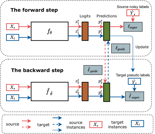
Figure 1: GearNet schematic. The forward step and the backward step are conducted iteratively. Each model is trained with a supervised learning loss on one domain, and a symmetric Kullback Leibler divergence loss to mimic the predictions of its dual model on the other domain, where $z_{*}^{*}$ is the logit coming from the last layer of the corresponding model, and $\boldsymbol{p}_{*}^{*}$ is the probability of classes calculated by the softmax function on $z_{*}^{*}$. Every time when the forward step stops, the pseudo labels of the target domain should be updated.

The Proposed GearNet

Problem statement. Throughout this paper, we consider the classification task under the setting of WSDA. We assume that we have a source domain with noisy labels corrupted from ground-truth labels $\hat{S}=\{(x_{i}^{s},\hat{y}_{i}^{s})\}_{i=1}^{n_{s}}$ and an unlabeled target domain $T=\{(x_{i}^{t})\}_{i=1}^{n_{t}}$, where $n_{s}$ and $n_{t}$ denote the number of instances from the source domain and the target domain respectively, and $\hat{y}_{i}^{s}$ denotes the noisy (corrupted) label. Our goal is to train a classifier $f_{\theta}:X\rightarrow Y$ based on $\hat{S}$ and $T$ to accurately annotate samples from the target domain.

As label noise will degenerate both the domain adaptation process (Yu et al. 2020) and the classification process (Zhang et al. 2016), existing methods (Shu et al. 2019; Liu et al. 2019; Yu et al. 2020) for WSDA focus on emphasizing useful samples by utilizing the supervision information from the source domain to reduce the negative impact of label noise. Considering the source domain could provide useful information to the target domain as mentioned above, we claim the target domain could also contain valuable information that is beneficial to the learning on the source domain. Therefore, inspired by the mutual learning (Zhang et al. 2018) and dual learning (Luo et al. 2019), we address the issue of WSDA by exploring the bilateral relationship that the two domains offer useful information to each other to handle domain shifts and label noise.

The intuition for exploring bilateral relationships in WSDA is briefly explained as follows. Similar to learning with label noise, existing WSDA methods would encounter the error accumulation issue: the error that comes from the biased selection of training instances in the previous iterations would be directly learnt again in the following training (Han et al. 2018). In WSDA, the accumulated error from learning with source domain examples would be amplified, causing a significant increase in the target domain error (Liu et al. 2019; Han et al. 2020). Co-teaching (Han et al. 2018) and Butterfly (Liu et al. 2019) alleviate this issue by training two networks with different initialization to exchange the biased selections with each other. In this work, our method introduce additional model diversity derived from the distinct supervision information by training two networks with opposite transfer directions. In this manner, the accumulated error would be further attenuated during the training stage.

1

input : Source dataset with noisy labels $\hat{S}$, target dataset with pseudo labels $\hat{T}$, max steps $M$, max epochs $N$, learning rate $\eta$, the pretrained basic model $f_{\theta}$ and its dual model $\tilde{f}_{\tilde{\theta}}$

output : $f_{\theta}$ and $\tilde{f}_{\tilde{\theta}}$

2

3for $t=0$ $\mathrm{to}$ $M$ do

4       Shuffle: $\hat{S}$ and $\hat{T}$;

       Initialize: $\tilde{f}_{\tilde{\theta}}$ ;

        // Start the backward step

5       for $i=0$ $\mathrm{to}$ $N$ do

6             Fetch: $\{x_{i}^{t},\hat{y}_{i}^{t}\}_{i=1}^{m_{t}}$ from $\hat{T}$, $\{x_{i}^{s}\}_{i=1}^{m_{s}}$ from $\hat{S}$;

7             Calculate: $\tilde{\ell}_{\mathrm{super}}=\frac{1}{m_{t}}\sum_{i=1}^{m_{t}}\ell(\hat{y}_{i}^{t},\tilde{f}(x_{i}^{t},\tilde{\theta})$);

8             Forward: $\boldsymbol{p}_{1}^{s}=f(x_{i}^{s},\theta)$, $\boldsymbol{p}_{2}^{s}=\tilde{f}(x_{i}^{s},\tilde{\theta})$;

9             Calculate: $\tilde{\ell}_{guide}$ by (7) using $\boldsymbol{p}_{1}^{s}$ and $\boldsymbol{p}_{2}^{s}$;

10             Obtain: $\tilde{\ell}_{total}$ by (3) ;

11             Update: $\tilde{\theta}=\tilde{\theta}-\eta\Delta\tilde{\ell}_{total}$;

12            

13       end for

14      

      Initialize: $f_{\theta}$ ;

        // Start the forward step

15       for $i=0$ $\mathrm{to}$ $N$ do

16             Fetch: $\{x_{i}^{s},\hat{y}_{i}^{s}\}_{i=1}^{m_{s}}$ from $\hat{S}$, $\{x_{i}^{t}\}_{i=1}^{m_{t}}$ from $\hat{T}$;

17             Calculate: $\ell_{\mathrm{super}}=\frac{1}{m_{s}}\sum_{i=1}^{m_{s}}\ell(\hat{y}_{i}^{s},f(x_{i}^{s},\theta)$);

18             Forward: $\boldsymbol{p}_{1}^{t}=f(x_{i}^{t},\theta)$, $\boldsymbol{p}_{2}^{t}=\tilde{f}(x_{i}^{t},\tilde{\theta})$;

19             Calculate: $\ell_{guide}$ by (6) using $\boldsymbol{p}_{1}^{t}$ and $\boldsymbol{p}_{2}^{t}$;

20             Obtain: $\ell_{total}$ by (3);

21             Update: $\theta=\theta-\eta\Delta\ell_{total}$;

22       end for

23      Update: $\{\hat{y}_{i}^{t}\}_{i=1}^{n_{t}}$ by $f_{\theta}$;

24 end for

Algorithm 1 GearNet’s Learning Strategy

Algorithm design. Inspired by the above motivation, we propose a universal paradigm called "GearNet" that can be employed to various backbone methods (i.e., existing WSDA methods). Before the introduction, we need to clarify at first that we omit the technical details of those backbone methods to simplify the introduction of GearNet, and assume that we build GearNet on the top of a basic backbone model that is composed of a feed-forward neural network. With this basic model, we can introduce GearNet in a more convenient way. After the introduction, we will further introduce how to employ GearNet to different backbone methods.

Our GearNet compromises two basic models: $f_{\theta}$ and $\tilde{f}_{\tilde{\theta}}$. Our model learning strategy includes three parts: the pretrained process aiming to annotate the target domain data by $f_{\theta}$ , the forward step aiming to transfer knowledge from the source domain to the target domain by $f_{\theta}$, and the backward step aiming to transfer knowledge from the target domain to the source domain by $\tilde{f}_{\tilde{\theta}}$. The forward step and the backward step are iteratively conducted until the whole training process ends.

In the pretrained process, we train $f_{\theta}$ on the source domain data with noisy labels $\hat{D}_{s}$ (i.e., Eq. (1)), and then use the model to generate the hard pseudo labels for the target domain instances (i.e., Eq. (2)).

$$\theta=\underset{\theta}{\operatorname{argmin}}\frac{1}{m_{s}}\sum\nolimits_{i=1}^{m_{s}}\ell(\hat{y}_{i}^{s},f(x_{i}^{s},\theta)),$$ (1)

$$\hat{y}_{i}^{t}=\underset{c}{\operatorname{argmax}}f_{c}(x_{i}^{t},\theta),\forall i=1,2,...,n_{t},$$ (2)

where $c$ denotes the $c$’th label, and $f_{c}$ is the network output for the $c$’th label.

Then the forward step and the backward step can be conducted in an opposite manner. In detail, both the forward and the backward step train their models with two losses: a conventional supervised learning loss (i.e., $\ell_{super}$ or $\tilde{\ell}_{super}$) on one domain and a mimicry loss that aligns predictions of the two models (i.e., $\ell_{guide}$ or $\tilde{\ell}_{guide}$) on the other domain. So their overall losses could be expressed as follows:

$$\ell_{\text{total}}=\ell_{\text{super}}+\beta\ell_{\text{guide}};\quad\tilde{\ell}_{\text{total}}=\tilde{\ell}_{\text{super}}+\beta\tilde{\ell}_{\text{guide}},$$ (3)

where $\beta$ is the trade-off hyperparameter, and its value is set as 0.1 in general. Besides, $\ell_{\text{total}}$ is for training $f_{\theta}$ during the forward step, while $\tilde{\ell}_{\text{total}}$ is for training $\tilde{f}_{\tilde{\theta}}$ during the backward step.

The supervised learning loss of the forward step is based on the noisy source domain:

$$\ell_{\mathrm{super}}=\frac{1}{m_{s}}\sum\nolimits_{i=1}^{m_{s}}\ell(\hat{y}_{i}^{s},f(x_{i}^{s},\theta)),$$ (4)

while that of the backward step is based on the pseudo-labeled target domain:

$$\tilde{\ell}_{\mathrm{super}}=\frac{1}{m_{t}}\sum\nolimits_{i=1}^{m_{t}}\ell(\hat{y}_{i}^{t},\tilde{f}(x_{i}^{t},\tilde{\theta})).$$ (5)

Although the model can perform well on the domain with supervision information due to the optimization of the supervised learning loss, there would be a significant accuracy drop on the test data from the other domain because of domain shifts. To generalize the model for better performance on the other domain, we introduce a consistency regularization, the symmetric Kullback-Leibler (KL) divergence loss (i.e., $\ell_{guide}$ or $\tilde{\ell}_{guide}$), which can enforce the model to mimic the predictions of its dual model for every sample from the other domain. So for the forward step, the loss is based on the target domain:

$$\ell_{\text{guide}}=D_{\mathrm{KL}}\left(\boldsymbol{p}_{1}^{t}\|\boldsymbol{p}_{2}^{t}\right)+D_{\mathrm{KL}}\left(\boldsymbol{p}_{2}^{t}\|\boldsymbol{p}_{1}^{t}\right),$$ (6)

For the backward step, the loss is calculated by the data from the source domain:

$$\tilde{\ell}_{\text{guide}}=D_{\mathrm{KL}}\left(\boldsymbol{p}_{1}^{s}\|\boldsymbol{p}_{2}^{s}\right)+D_{\mathrm{KL}}\left(\boldsymbol{p}_{2}^{s}\|\boldsymbol{p}_{1}^{s}\right).$$ (7)

$D_{\mathrm{KL}}$ denotes the Kullback-Leibler (KL) divergence that measures the probability difference (Kullback and Leibler 1951):

$$D_{\mathrm{KL}}\left(p\|q\right)=\sum_{i=1}^{n}p(x_{i})log\frac{p(x_{i})}{q(x_{i})},$$ (8)

where $p$ and $q$ denote the probability to be measured for the probability difference, and $n$ is the number of samples.

In the forward step, the consistency regularization is obtained by inputting $\boldsymbol{p}_{1}^{t}$ and $\boldsymbol{p}_{2}^{t}$ into Eq. (8), where $\boldsymbol{p}_{1}^{t}$ and $\boldsymbol{p}_{2}^{t}$ denotes class label distributions which are outputs from $f_{\theta}$ and $\tilde{f}_{\tilde{\theta}}$, respectively. In the backward step, the consistency regularization is calculated by inputting $\boldsymbol{p}_{1}^{s}$ and $\boldsymbol{p}_{2}^{s}$, where $\boldsymbol{p}_{1}^{s}$ and $\boldsymbol{p}_{2}^{s}$ denote the class label distributions which are outputs from $f_{\theta}$ and $\tilde{f}_{\tilde{\theta}}$, respectively. Every factor in those probability metrics is computed by the softmax function based on the corresponding logits. For example, the probability of class $c$ for the sample $x_{i}^{s}$ from $f_{\theta}$ (i.e., $p_{1}^{c}(x_{i}^{s})$) is calculated as:

$$p_{1}^{c}(x_{i}^{s})=\frac{exp(z_{1}^{c})}{\sum_{c^{{}^{\prime}}=1}^{C}exp(z_{1}^{c^{{}^{\prime}}})},$$ (9)

where $z_{1}^{c}$ denotes the logit of class $c$ from $f_{\theta}$ for $x_{i}^{s}$.

Optimisation of GearNet. After the pretrained process to provide pseudo labels to the target domain, the whole algorithm is run as Algorithm 1 and Figure 1. We first conduct the backward step by computing the total loss $\tilde{\ell}_{total}$ as Eq. (3) for training $\tilde{f}_{\tilde{\theta}}$, where the second loss $\tilde{\ell}_{guide}$ is between $\tilde{f}_{\tilde{\theta}}$ and the pre-trained $f_{\theta}$ on the source domain. Then we can continue to update the parameters of $f_{\theta}$ in the forward step by the total loss $\ell_{total}$ also as Eq. (3), where the mimicry loss $\ell_{guide}$ is between the initialized $f_{\theta}$ and $\tilde{f}_{\tilde{\theta}}$ trained during the backward step on the target domain, after which we update the pseudo labels of the target domain by the trained $f_{\theta}$. We repeat the forward and the backward steps until this algorithm stops. It is worthy to note that the training model should be initialized before its training process to avoid overfitting to the noisy samples.

Tasks	$A\rightarrow W$	$A\rightarrow D$	$W\rightarrow A$	$W\rightarrow D$	$D\rightarrow A$	$D\rightarrow W$	Average
Standard	$46.61\pm 0.32$	$51.46\pm 0.53$	$44.21\pm 0.12$	$73.13\pm 0.26$	$43.43\pm 0.32$	$65.63\pm 0.41$	$54.06\pm 0.33$
Co-teaching	$49.87\pm 1.42$	$55.00\pm 0.89$	$42.18\pm 0.71$	$75.63\pm 0.85$	$44.85\pm 1.01$	$64.06\pm 2.01$	$55.98\pm 1.15$
JoCoR	$50.53\pm 1.67$	$55.42\pm 2.33$	$47.19\pm 1.71$	$74.79\pm 1.28$	$44.50\pm 1.01$	$61.72\pm 0.98$	$55.69\pm 1.50$
DAN	$54.39\pm 2.11$	$54.79\pm 1.32$	$36.65\pm 2.62$	$67.08\pm 1.79$	$35.09\pm 1.58$	$60.94\pm 2.06$	$51.32\pm 1.91$
DANN	$50.91\pm 1.88$	$54.17\pm 0.87$	$44.57\pm 0.74$	$74.79\pm 1.08$	$45.35\pm 1.41$	$67.58\pm 0.48$	$56.23\pm 1.08$
TCL	$56.46\pm 0.67$	$63.13\pm 1.14$	$45.31\pm 0.31$	$76.87\pm 0.85$	$44.78\pm 0.60$	$71.22\pm 0.58$	$59.63\pm 0.69$
$\text{GearNet}_{\text{Co-teaching}}$	$53.12\pm 1.88$	$58.12\pm 1.11$	$44.49\pm 0.57$	$76.87\pm 1.94$	49.28$\pm$1.37	$69.14\pm 1.81$	$56.75\pm 1.44$
$\text{GearNet}_{\text{DANN}}$	60.68 $\pm$ 0.26	$63.54\pm 1.03$	$47.19\pm 0.96$	$76.88\pm 1.68$	47.90 $\pm$ 0.66	$72.39\pm 0.79$	$61.43\pm 0.90$
$\text{GearNet}_{\text{TCL}}$	$58.84\pm 0.57$	65.63 $\pm$ 0.93	48.37 $\pm$ 1.04	78.54 $\pm$ 0.75	$47.80\pm 0.58$	73.44 $\pm$ 0.56	62.10 $\pm$ 0.74

Table 1: Target accuracy (%) on Office-31 datasets with Unif-20% noise. Bold numbers are superior results

Realizations of GearNet. In this subsection, we incorporate three backbone methods with GearNet as examples. They are Co-teaching (Han et al. 2018) that belongs to the approach to improve model robustness against label noise, DANN (Ganin et al. 2016) that belongs to the domain adaptation approach and TCL (Shu et al. 2019) that belongs to the WSDA approach, respectively. All the three algorithms are representative approaches, which could spotlight the universal capability of GearNet.

First of all, we also need to initialize two models $f_{\theta}$ and $\tilde{f}_{\tilde{\theta}}$ with the backbone algorithm. Although these backbone methods have different learning strategies, we generally express their loss functions as follows to highlight the structure of GearNet:

$$\ell_{bone}=\mathbb{E}_{p^{s}(x^{s},\hat{y^{s}}),p^{t}(x^{t})}(\ell(x^{s},\hat{y^{s}},x^{t};f_{\theta})),$$ (10)

$$\tilde{\ell}_{bone}=\mathbb{E}_{p^{t}(x^{t},\hat{y^{t}}),p^{s}(x^{s})}(\ell(x^{t},\hat{y^{t}},x^{s};\tilde{f}_{\tilde{\theta}})),$$ (11)

where $\ell_{bone}$ denotes the loss of the backbone method for training $f_{\theta}$, while $\tilde{\ell}_{bone}$ denotes the same meaning for training $\tilde{f}_{\tilde{\theta}}$. Besides, $p^{s}(*)$ and $p^{t}(*)$ denote the distribution from the source domain, and the target domain, respectively.

The two losses above take the place of $\ell_{super}$ and $\tilde{\ell}_{super}$ in Eq. (3) when we chose those backbone methods. They represent different meanings under various backbone algorithms. For the Co-teaching backbone method, they reduce the impact of noise by cross-updating two peer networks. As for DANN, they decrease the domain discrepancy using a domain discriminator in an adversarial manner. For TCL, they address both the label noise problem and the domain shift problem by selecting noiseless and transferable samples from the source domain to train the DANN-shape model.

To obtain $\ell_{guide}$ and $\tilde{\ell}_{guide}$, the training model should align its predictions with corresponding class posteriors of its dual model. Note that only classification predictions need to be aligned. Besides, for multi-classifier models, like Co-teaching, these losses should be computed for every classifier with the dual model, so that all of them can have the professional guidance on the domain that they are not good at.

Relation to CycleGAN. CyCADA (Hoffman et al. 2018) and Bi-Directional Generation domain adaptation model (BGD) (Yang et al. 2020) also propose the idea that transfers knowledge from the target domain to the the source domain, which are inspired by CycleGAN (Zhu et al. 2017). They transfer the instances of the target domain to that of the source domain by a feature generator, which aim is to obtain a feature space that is close to the source domain. However, there are fundamental differences between them and GearNet. (i) CyCADA and BGD obtain a feature generator that can convert the target-style feature to the source-style feature, but GearNet trains a model that leverages the target domain to predict labels of the source domain. (ii) The reason why CyCADA and BGD transfer the feature style is to predict the labels of the target domain using the classifier trained by the source domain. But GearNet aims to exploit information from the target domain which could enhance both the domain adaptation process and the noise reduction process for the source domain. (iii) CyCADA and BGD address the issue of unsupervised domain adaptation, but GearNet handles the issue of weakly-supervised domain adaptation.

Relation to multi-task learning. In the problem of multi-task learning, there is also an idea that a noisy task can reduce its noise under the assistance of another noisy task (Wu, Zhang, and Ré 2020). However, the crucial difference between multi-task learning and GearNet is that multi-task learning aims at good performance for all the tasks, but GearNet only needs to achieve good performance for the target domain. In addition, the above idea for multi-task learning proposes that more noisy tasks can reduce the impact of noise and get better performance by up weighting less noisy tasks, but GearNet proposes that both the target domain and the source domain contain useful knowledge for each other.

Experiments

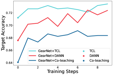
(a)

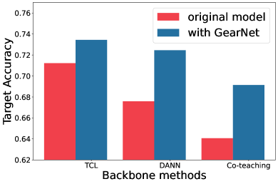
(b)

Figure 3: Universal capability of GearNet on $D\rightarrow W$ with Unif-20% noise under WSDA (TCL), de-noise (Co-teaching) and UDA (DANN) backbone methods. (a) Trend of target accuracy across training steps. (b) Best target accuracy across training steps

Tasks	$A\rightarrow W$	$A\rightarrow D$	$W\rightarrow A$	$W\rightarrow D$	$D\rightarrow A$	$D\rightarrow W$	Average
Standard	$34.37\pm 0.78$	$36.45\pm 0.43$	$29.26\pm 0.52$	$54.79\pm 0.72$	$30.79\pm 0.95$	$48.31\pm 0.69$	$40.00\pm 0.68$
Co-teaching	$36.20\pm 2.45$	$41.04\pm 1.42$	$31.11\pm 1.64$	$53.13\pm 1.91$	$23.08\pm 1.63$	$38.93\pm 2.63$	$37.25\pm 1.95$
JoCoR	$37.11\pm 1.27$	$42.29\pm 2.24$	$28.98\pm 1.78$	$47.50\pm 1.89$	$23.40\pm 2.09$	$36.85\pm 2.74$	$36.02\pm 2.00$
DAN	$34.24\pm 1.73$	$35.83\pm 2.42$	$23.97\pm 2.89$	$47.71\pm 1.99$	$24.96\pm 2.07$	$41.02\pm 1.79$	$34.62\pm 2.15$
DANN	$36.20\pm 1.62$	$40.20\pm 1.27$	$30.22\pm 1.53$	$54.38\pm 1.59$	$32.71\pm 2.06$	$49.74\pm 1.82$	$40.57\pm 1.65$
TCL	$42.06\pm 1.86$	$46.04\pm 2.68$	$29.55\pm 0.96$	$54.38\pm 1.74$	$30.43\pm 1.83$	$49.09\pm 2.62$	$41.95\pm 1.95$
$\text{GearNet}_{\text{Co-teaching}}$	$39.32\pm 1.07$	$43.33\pm 0.97$	33.94 $\pm$ 1.07	$56.04\pm 1.31$	$25.74\pm 1.58$	$38.41\pm 1.30$	$39.46\pm 1.21$
$\text{GearNet}_{\text{DANN}}$	$43.48\pm 1.45$	48.54 $\pm$ 1.72	$30.45\pm 1.37$	58.54 $\pm$ 1.86	35.51 $\pm$ 0.83	54.17 $\pm$ 1.06	45.12 $\pm$ 1.38
$\text{GearNet}_{\text{TCL}}$	46.61 $\pm$ 0.89	$47.50\pm 1.28$	$30.39\pm 2.01$	$55.83\pm 1.92$	$28.91\pm 1.47$	$52.47\pm 1.39$	$43.62\pm 1.49$

Table 2: Target accuracy (%) on Office-31 datasets with Unif-40% noise. Bold numbers are superior results.

Tasks	$A\rightarrow W$	$A\rightarrow D$	$W\rightarrow A$	$W\rightarrow D$	$D\rightarrow A$	$D\rightarrow W$	Average
Standard	$46.61\pm 0.92$	$46.67\pm 1.83$	$41.41\pm 0.94$	$69.17\pm 1.03$	$40.23\pm 1.06$	$64.19\pm 0.74$	$51.38\pm 1.08$
Co-teaching	$48.31\pm 2.01$	$50.21\pm 1.37$	$42.19\pm 1.87$	$69.17\pm 2.40$	$39.20\pm 1.82$	$58.59\pm 2.72$	$51.28\pm 2.03$
JoCoR	$49.74\pm 0.98$	$51.46\pm 1.52$	$41.94\pm 1.83$	$67.92\pm 2.07$	$37.71\pm 1.68$	$55.86\pm 0.93$	$50.77\pm 1.50$
DAN	$56.64\pm 1.73$	$53.54\pm 2.04$	$40.20\pm 2.13$	$70.21\pm 1.57$	$35.80\pm 1.78$	$64.84\pm 1.84$	$53.54\pm 1.85$
DANN	$47.66\pm 1.46$	$50.63\pm 1.76$	$39.17\pm 0.63$	$69.58\pm 1.05$	$41.55\pm 0.77$	$65.49\pm 0.86$	$52.35\pm 1.09$
TCL	$55.99\pm 1.79$	$61.04\pm 1.53$	$42.37\pm 2.51$	$72.92\pm 0.62$	$42.29\pm 1.33$	$70.96\pm 2.52$	$57.60\pm 1.72$
$\text{GearNet}_{\text{Co-teaching}}$	$51.95\pm 1.33$	$54.37\pm 1.13$	$44.49\pm 1.80$	$71.87\pm 0.93$	$41.79\pm 1.71$	$61.45\pm 0.97$	$54.32\pm 1.31$
$\text{GearNet}_{\text{DANN}}$	59.51 $\pm$ 1.58	$61.25\pm 0.63$	$41.44\pm 1.96$	$72.08\pm 1.05$	$44.89\pm 1.58$	$69.27\pm 1.62$	$58.07\pm 1.40$
$\text{GearNet}_{\text{TCL}}$	$58.85\pm 0.96$	62.71 $\pm$ 0.73	44.28 $\pm$ 1.53	75.00 $\pm$ 1.67	45.03 $\pm$ 0.85	75.00 $\pm$ 1.09	60.15 $\pm$ 1.14

Table 3: Target accuracy (%) on Office-31 datasets with Flip-20% noise. The best results are highlighted in bold.

Tasks	$A\rightarrow W$	$A\rightarrow D$	$W\rightarrow A$	$W\rightarrow D$	$D\rightarrow A$	$D\rightarrow W$	Average
Standard	$35.93\pm 1.09$	$37.50\pm 1.14$	$30.39\pm 1.21$	$53.96\pm 1.04$	$29.83\pm 1.81$	$46.88\pm 1.35$	$39.08\pm 1.27$
Co-teaching	$35.94\pm 1.97$	$37.92\pm 2.48$	$28.13\pm 2.09$	$49.17\pm 1.35$	$26.03\pm 1.71$	$37.76\pm 1.95$	$35.82\pm 1.93$
JoCoR	$36.07\pm 1.85$	$37.29\pm 1.27$	$27.73\pm 1.88$	$48.12\pm 2.08$	$26.35\pm 1.11$	$38.28\pm 1.60$	$35.64\pm 1.63$
DAN	$43.49\pm 1.17$	$41.46\pm 2.14$	$30.61\pm 1.43$	$53.54\pm 2.01$	$28.94\pm 2.36$	$50.39\pm 2.35$	$41.41\pm 1.91$
DANN	$36.98\pm 1.84$	$40.42\pm 1.89$	$30.26\pm 2.04$	$53.33\pm 2.58$	$30.36\pm 1.52$	$44.66\pm 1.92$	$39.96\pm 1.96$
TCL	$44.79\pm 0.98$	$43.75\pm 1.57$	$30.82\pm 1.37$	$54.17\pm 1.90$	$29.97\pm 1.86$	$45.96\pm 1.37$	$41.58\pm 1.51$
$\text{GearNet}_{\text{Co-teaching}}$	$40.36\pm 0.85$	$38.75\pm 1.14$	$30.39\pm 0.58$	$51.04\pm 1.17$	$27.37\pm 0.64$	$40.23\pm 1.36$	$38.02\pm 0.96$
$\text{GearNet}_{\text{DANN}}$	$42.45\pm 1.33$	$42.08\pm 1.54$	31.21 $\pm$ 1.73	54.38 $\pm$ 1.48	31.35 $\pm$ 0.79	$45.96\pm 1.63$	$41.24\pm 1.42$
$\text{GearNet}_{\text{TCL}}$	48.69 $\pm$ 1.02	46.25 $\pm$ 1.46	$30.64\pm 1.58$	$53.96\pm 1.24$	$31.00\pm 0.89$	47.79 $\pm$ 1.24	43.06 $\pm$ 1.24

Table 4: Target accuracy (%) on Office-31 datasets with Flip-40% noise. Bold numbers are superior results.

Tasks	Standard	Co-teaching	JoCoR	DAN	DANN	TCL	$\text{GearNet}_{\text{Co-teaching}}$	$\text{GearNet}_{\text{DANN}}$	$\text{GearNet}_{\text{TCL}}$
$Ar\rightarrow CI$	24.51$\pm$1.82	26.49$\pm$1.40	26.60$\pm$1.93	23.12$\pm$0.90	26.41$\pm$1.51	26.48$\pm$0.93	27.82$\pm$0.42	27.30$\pm$1.07	28.01$\pm$0.75
$Ar\rightarrow Pr$	42.41$\pm$1.59	45.15$\pm$1.79	45.08$\pm$2.02	33.94$\pm$0.95	41.13$\pm$1.20	42.75$\pm$1.06	52.15$\pm$0.73	47.01$\pm$1.05	46.58$\pm$0.93
$Ar\rightarrow Rw$	48.75$\pm$1.89	51.51$\pm$1.67	51.56$\pm$2.28	50.33$\pm$1.10	49.60$\pm$1.66	49.63$\pm$1.12	54.71$\pm$0.70	51.12$\pm$1.15	52.33$\pm$1.50
$CI\rightarrow Ar$	27.58$\pm$1.60	27.70$\pm$1.17	27.91$\pm$1.76	26.11$\pm$0.65	34.08$\pm$1.67	36.22$\pm$0.96	31.20$\pm$0.77	36.34$\pm$0.82	37.37$\pm$1.47
$CI\rightarrow Pr$	34.60$\pm$1.09	35.39$\pm$1.63	34.98$\pm$1.48	31.61$\pm$1.18	38.22$\pm$2.21	41.89$\pm$1.30	42.77$\pm$0.75	43.09$\pm$0.98	43.22$\pm$0.91
$CI\rightarrow Rw$	37.59$\pm$1.45	26.08$\pm$1.07	37.20$\pm$1.43	34.28$\pm$1.40	42.41$\pm$1.63	45.35$\pm$1.48	43.01$\pm$0.84	44.78$\pm$0.56	46.48$\pm$0.86
$Pr\rightarrow Ar$	29.33$\pm$0.83	32.12$\pm$1.31	32.08$\pm$1.34	25.12$\pm$0.57	34.62$\pm$1.71	35.15$\pm$1.40	33.92$\pm$1.22	36.75$\pm$0.83	37.58$\pm$1.27
$Pr\rightarrow CI$	23.18$\pm$1.68	23.92$\pm$0.60	24.11$\pm$1.59	23.47$\pm$1.78	24.00$\pm$1.70	25.79$\pm$0.69	23.72$\pm$1.13	24.11$\pm$1.10	28.46$\pm$1.42
$Pr\rightarrow Rw$	46.07$\pm$1.91	48.32$\pm$1.07	48.80$\pm$1.39	40.92$\pm$1.00	49.65$\pm$1.56	52.68$\pm$1.55	50.22$\pm$0.69	50.89$\pm$1.05	54.84$\pm$1.11
$Rw\rightarrow Ar$	41.37$\pm$1.58	43.20$\pm$1.35	44.03$\pm$1.84	35.48$\pm$1.09	43.66$\pm$2.14	44.98$\pm$0.84	44.37$\pm$0.91	44.61$\pm$0.56	46.54$\pm$1.49
$Rw\rightarrow CI$	26.76$\pm$1.89	28.12$\pm$1.36	28.55$\pm$1.59	27.14$\pm$0.73	28.30$\pm$1.10	29.03$\pm$1.92	28.54$\pm$1.12	28.80$\pm$1.03	31.06$\pm$1.38
$Rw\rightarrow Pr$	51.76$\pm$1.71	53.94$\pm$1.58	53.87$\pm$1.29	46.15$\pm$1.46	51.88$\pm$1.79	54.84$\pm$1.06	55.19$\pm$1.27	53.98$\pm$1.27	57.24$\pm$1.16
Average	36.16$\pm$1.59	36.83$\pm$1.34	37.90$\pm$1.65	33.14$\pm$1.05	38.66$\pm$1.20	40.40$\pm$1.19	40.64$\pm$0.87	40.73$\pm$0.96	42.48$\pm$1.19

Table 5: Target accuracy (%) on Office-Home datasets with Unif-20% noise. The best results are highlighted in bold.

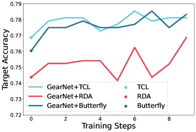
(a)

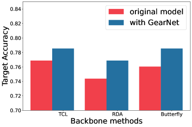
(b)

Figure 5: Universal capability of GearNet on $W\rightarrow D$ with Unif-20% noise for three different WSDA (TCL, RDA, Butterfly) backbone methods. (a) Trend of target accuracy across training steps. (b) Best target accuracy across training steps.

Experimental setup

We compare GearNet with 6 state-of-the-art baselines, implement all methods by PyTorch, and conduct all the experiments on NVIDIA Tesla V100 GPU. Their details are as follows: Standard (He et al. 2016), which is a neural network classifier constructed by the pre-trained ResNet-50. Note that ResNet-50 is also used as the feature extractor of the following benchmarks for comparability. DANN (Ganin et al. 2016), which is constructed by a feature extractor, a classification layer and a domain discriminator. The feature extractor generates a feature space that can confuse the domain discriminator, so that it can decrease the domain discrepancy. DAN (Long et al. 2015), which proposes MK-MMD as the domain discrepancy measure to reduce the difference between the two domains. Co-teaching (Han et al. 2018), which trains and cross-updates two peer networks simultaneously to combat label noise. JoCoR (Wei et al. 2020), which trains two neural networks simultaneously and calculates a joint loss with Co-regularization to merge their outputs between the two neural networks in order to improve the model robustness against label noise. TCL (Shu et al. 2019), which selects transferable and noiseless samples from the source domain to train a model with the same structure as DANN to handle the WSDA issue. RDA (Han et al. 2020), which proposes an offline curriculum learning to select clean samples from the source domain and a proxy margin discrepancy to eliminate the negative impact of label noise. Butterfly (Liu et al. 2019), which picks clean samples from both of the two domains to train two Co-teaching models simultaneously.

We simulate experiments based on Office-31 (Saenko et al. 2010) and Office-Home (Venkateswara et al. 2017). The first dataset is a classical dataset for domain adaptation, which contains 4,652 images with 31 classes. Three various domains are contained in the dataset: Amazon (A), Webcam (W) and DSLR (D). They represent that images are collected from amazon.com, web camera and digital SLR camera, respectively. The second dataset consists of 4 domains: Artistic (Ar), Clip Art (Cl), Product (Pr) and Real-World (Rw) containing 15,500 images with 65 classes. They represent different image styles that are artistic depictions, clipart images, images without background and pictures captured by cameras, respectively. We manually inject two types of noisy labels for the source domain: uniform noise (Zhang et al. 2020) and asymmetry flipping noise (Patrini et al. 2017), and their details are in the supplemental document.

For comparability, all the experiments use Stochastic gradient descent optimizer with an initial learning rate of 0.003 and a momentum of 0.9. The batch size is set as 32 and the total number of epochs is 200. For GearNet, the total number of steps is set as 10. To measure the performance, we evaluate the target accuracy by all the samples from the target domain, i.e., target accuracy = (# of correct target predictions)/(# of target domain data). All the experiments are repeated 5 times with different seeds, and we report the average accuracy and their standard deviation on tables.

Numerical results

Results on Office-31. Table 1, Table 2, Table 3 and Table 4 report the target-domain accuracy in 6 digit tasks that are combined in pairs by the three domains from Office-31 under different types and levels of noise.

Table 1 and Table 3 represent two simpler cases, since their noise rate is 20%. The two tables illustrate that our method is able to improve existing backbone methods significantly when the noise rate is low. Table 2 and Table 4 represent two harder cases with 40% noise rate. The two tables show that GearNet can enhance the performance of original algorithms on most tasks when the noise rate is high. GearNet obtains comparable results on the tasks of $D\rightarrow A$ and $W\rightarrow A$. The reason is that Webcam and DSLR are two small datasets compared with Amazon, so that it is ineffective to transfer knowledge from Webcam or DSLR to Amazon under 40% noise rate. When we explore pseudo supervision information from Amazon based on the pseudo labels provided by the two small datasets, it is more likely to explore negative information and transfer it back to Amazon. However, when the noise rate becomes 20%, all the tasks can be improved by GearNet, since all of the source domains are capable to provide adequate transferable information to their target domains and vise versa.

To show the universal capability of GearNet on backbone methods from different fields, we draw Fig. 3. The left figure illustrates the trend of target accuracy of GearNet across training steps under the three backbone methods. The step 0 refers to the pretrained process, the even number step (i.e., step 2, 4, …) refers the forward step from the source domain to the target domain, and the odd number step (i.e., step 1, 3, 5, …) means the backward step from the target domain to the source domain. Specifically, the value of the first point denotes the target accuracy of the original backbone model. The right figure illustrates the performance improvement before and after we incorporate GearNet with the three methods. From the figures, we can observe that GearNet can continuously enhance the performance of the backbone methods. The figures on $D\rightarrow W$ with Unif-40% noise, Flip-20% noise and Flip-40% noise are in the supplemental document.

	$\text{GearNet}_{\text{Co-teaching}}$		$\text{GearNet}_{\text{DANN}}$		$\text{GearNet}_{\text{TCL}}$
Tasks	w/o	w/	w/o	w/	w/o	w/
$D\rightarrow W\quad\text{Unif-20}\%$	67.58	69.14	70.18	72.39	71.74	73.44
$D\rightarrow W\quad\text{Unif-40}\%$	36.58	38.41	49.09	54.17	49.47	52.47
$Ar\rightarrow Cl\quad\text{Unif-20}\%$	27.39	27.82	26.53	27.30	26.41	28.01
$Ar\rightarrow Cl\quad\text{Unif-40}\%$	18.65	18.75	17.56	17.58	16.30	17.93

Table 6: Results of ablation study on various tasks with Uniform noise. The best results are highlighted in bold.

To illustrate the universal capability of GearNet on different WSDA methods, we incorporate three WSDA methods with GearNet including TCL (Shu et al. 2019), Butterfly (Liu et al. 2019) and RDA (Han et al. 2020) based on the Office-31 benchmark dataset (source: Webcam; target: DSLR). Their results are shown in Fig. 5. The two figures illustrate that GearNet can also significantly improve the prediction accuracy on the target domain for various WSDA methods.

Results on Office-Home. Table 5 report the average target accuracy on 12 tasks that are combined in pairs by the 4 domains from Office-Home when the uniform noise rate is 20%. This table shows that GearNet can significantly improve the performance compared with original models. Especially, in the case of $Ar\rightarrow Pr$, the target accuracy is from 42% to 52% when the backbone method is Co-teaching, which is a significant improvement.

Ablation study

To illustrate the importance of the consistency regularization (i.e., $\ell_{guide}$ and $\tilde{\ell}_{guide}$), we conduct an ablation study on four tasks, and the results are shown in Table 6. The backbone algorithms are Co-teaching (Han et al. 2018), DANN (Ganin et al. 2016) and TCL (Shu et al. 2019), which represent a de-noise method, a domain adaptation method and a WSDA method, respectively. From Table 6, it is clear to see that the guidance on the testing domain from the other model could significantly improve the performance of the classification for most of the methods.

Conclusion

In this paper, we propose a universal paradigm called GearNet that enhances many existing robust training methods to address the issue of weakly-supervised domain adaptation. To the best of our knowledge, our method is the first to explore the benefit of utilizing pseudo supervision knowledge from the target domain in improving the robustness against noisy labels from the source domain. We show that exploring bilateral relationships would further improve the generalization performance when the labels from the source domain are noisy. Extensive experiments show that GearNet is easy to be integrated into existing algorithms and these methods equipped with GearNet can significantly outperform their original performance. Overall, our method is an effective and complementary approach for boosting robustness against noisy labels in the setting of domain adaptation.

References

- Blitzer, McDonald, and Pereira (2006) Blitzer, J.; McDonald, R.; and Pereira, F. 2006. Domain adaptation with structural correspondence learning. In Proceedings of the 2006 Conference on Empirical Methods in Natural Language Processing, 120–128.
- Chen et al. (2020) Chen, Y.; Wei, C.; Kumar, A.; and Ma, T. 2020. Self-training avoids using spurious features under domain shift. arXiv preprint arXiv:2006.10032.
- Combes et al. (2020) Combes, R. T. d.; Zhao, H.; Wang, Y.-X.; and Gordon, G. 2020. Domain adaptation with conditional distribution matching and generalized label shift. arXiv preprint arXiv:2003.04475.
- Dong et al. (2021a) Dong, J.; Cong, Y.; Sun, G.; Fang, Z.; and Ding, Z. 2021a. Where and How to Transfer: Knowledge Aggregation-Induced Transferability Perception for. Unsupervised Domain Adaptation. IEEE Transactions on Pattern Analysis and Machine Intelligence.
- Dong et al. (2020) Dong, J.; Cong, Y.; Sun, G.; Zhong, B.; and Xu, X. 2020. What Can Be Transferred: Unsupervised Domain Adaptation for Endoscopic Lesions Segmentation. In IEEE/CVF Conference on Computer Vision and Pattern Recognition (CVPR), 4022–4031.
- Dong et al. (2021b) Dong, J.; Fang, Z.; Liu, A.; Sun, G.; and Liu, T. 2021b. Confident-anchor-induced multi-source-free domain adaptation. In NeurIPS.
- Fang et al. (2021a) Fang, Z.; Lu, J.; Liu, A.; Liu, F.; and Zhang, G. 2021a. Learning Bounds for Open-Set Learning. In ICML, 3122–3132.
- Fang et al. (2021b) Fang, Z.; Lu, J.; Liu, F.; Xuan, J.; and Zhang, G. 2021b. Open Set Domain Adaptation: Theoretical Bound and Algorithm. IEEE Trans. Neural Networks Learn. Syst., 4309–4322.
- Feng et al. (2020) Feng, L.; Shu, S.; Lin, Z.; Lv, F.; Li, L.; and An, B. 2020. Can cross entropy loss be robust to label noise? In International Joint Conference on Artificial Intelligence, 2206–2212.
- Frénay and Verleysen (2013) Frénay, B.; and Verleysen, M. 2013. Classification in the presence of label noise: a survey. IEEE Transactions on Neural Networks and Learning Systems, 25(5): 845–869.
- Ganin et al. (2016) Ganin, Y.; Ustinova, E.; Ajakan, H.; Germain, P.; Larochelle, H.; Laviolette, F.; Marchand, M.; and Lempitsky, V. 2016. Domain-adversarial training of neural networks. The Journal of Machine Learning Research, 17(1): 2096–2030.
- Ghafoorian et al. (2017) Ghafoorian, M.; Mehrtash, A.; Kapur, T.; Karssemeijer, N.; Marchiori, E.; Pesteie, M.; Guttmann, C. R.; de Leeuw, F.-E.; Tempany, C. M.; Van Ginneken, B.; et al. 2017. Transfer learning for domain adaptation in mri: Application in brain lesion segmentation. In International Conference on Medical Image Computing and Computer-assisted Intervention, 516–524. Springer.
- Ghosh, Kumar, and Sastry (2017) Ghosh, A.; Kumar, H.; and Sastry, P. 2017. Robust loss functions under label noise for deep neural networks. In Proceedings of the AAAI Conference on Artificial Intelligence, volume 31, 1919––1925.
- Goldberger and Ben-Reuven (2016) Goldberger, J.; and Ben-Reuven, E. 2016. Training deep neural-networks using a noise adaptation layer. In Proceedings of the 5th International Conference on Learning Representation.
- Han et al. (2018) Han, B.; Yao, Q.; Yu, X.; Niu, G.; Xu, M.; Hu, W.; Tsang, I.; and Sugiyama, M. 2018. Co-teaching: Robust training of deep neural networks with extremely noisy labels. arXiv preprint arXiv:1804.06872.
- Han, Luo, and Wang (2019) Han, J.; Luo, P.; and Wang, X. 2019. Deep self-learning from noisy labels. In Proceedings of the IEEE/CVF International Conference on Computer Vision, 5138–5147.
- Han et al. (2020) Han, Z.; Gui, X.-J.; Cui, C.; and Yin, Y. 2020. Towards Accurate and Robust Domain Adaptation under Noisy Environments. arXiv preprint arXiv:2004.12529.
- He et al. (2016) He, K.; Zhang, X.; Ren, S.; and Sun, J. 2016. Deep residual learning for image recognition. In Proceedings of the IEEE Conference on Computer Vision and Pattern Recognition, 770–778.
- Hoffman et al. (2014) Hoffman, J.; Guadarrama, S.; Tzeng, E.; Hu, R.; Donahue, J.; Girshick, R.; Darrell, T.; and Saenko, K. 2014. LSDA: Large scale detection through adaptation. arXiv preprint arXiv:1407.5035.
- Hoffman et al. (2018) Hoffman, J.; Tzeng, E.; Park, T.; Zhu, J.-Y.; Isola, P.; Saenko, K.; Efros, A.; and Darrell, T. 2018. Cycada: Cycle-consistent adversarial domain adaptation. In International Conference on Machine Learning, 1989–1998. PMLR.
- Jiang et al. (2018) Jiang, L.; Zhou, Z.; Leung, T.; Li, L.-J.; and Fei-Fei, L. 2018. Mentornet: Learning data-driven curriculum for very deep neural networks on corrupted labels. In International Conference on Machine Learning, 2304–2313. PMLR.
- Kamnitsas et al. (2017) Kamnitsas, K.; Baumgartner, C.; Ledig, C.; Newcombe, V.; Simpson, J.; Kane, A.; Menon, D.; Nori, A.; Criminisi, A.; Rueckert, D.; et al. 2017. Unsupervised domain adaptation in brain lesion segmentation with adversarial networks. In International Conference on Information Processing in Medical Imaging, 597–609. Springer.
- Kullback and Leibler (1951) Kullback, S.; and Leibler, R. A. 1951. On information and sufficiency. The Annals of Mathematical Statistics, 22(1): 79–86.
- Lee and Raginsky (2017) Lee, J.; and Raginsky, M. 2017. Minimax statistical learning with wasserstein distances. arXiv preprint arXiv:1705.07815.
- Liu et al. (2019) Liu, F.; Lu, J.; Han, B.; Niu, G.; Zhang, G.; and Sugiyama, M. 2019. Butterfly: A panacea for all difficulties in wildly unsupervised domain adaptation. arXiv preprint arXiv:1905.07720.
- Long et al. (2015) Long, M.; Cao, Y.; Wang, J.; and Jordan, M. 2015. Learning transferable features with deep adaptation networks. In International Conference on Machine Learning, 97–105. PMLR.
- Luo et al. (2019) Luo, F.; Li, P.; Zhou, J.; Yang, P.; Chang, B.; Sui, Z.; and Sun, X. 2019. A dual reinforcement learning framework for unsupervised text style transfer. arXiv preprint arXiv:1905.10060.
- Menon et al. (2015) Menon, A.; Van Rooyen, B.; Ong, C. S.; and Williamson, B. 2015. Learning from corrupted binary labels via class-probability estimation. In International Conference on Machine Learning, 125–134. PMLR.
- Pan et al. (2010) Pan, S. J.; Tsang, I. W.; Kwok, J. T.; and Yang, Q. 2010. Domain adaptation via transfer component analysis. IEEE Transactions on Neural Networks, 22(2): 199–210.
- Pan and Yang (2009) Pan, S. J.; and Yang, Q. 2009. A survey on transfer learning. IEEE Transactions on Knowledge and Data Engineering, 22(10): 1345–1359.
- Patrini et al. (2017) Patrini, G.; Rozza, A.; Krishna Menon, A.; Nock, R.; and Qu, L. 2017. Making deep neural networks robust to label noise: A loss correction approach. In Proceedings of the IEEE Conference on Computer Vision and Pattern Recognition, 1944–1952.
- Ren et al. (2018) Ren, M.; Zeng, W.; Yang, B.; and Urtasun, R. 2018. Learning to reweight examples for robust deep learning. In International Conference on Machine Learning, 4334–4343. PMLR.
- Saenko et al. (2010) Saenko, K.; Kulis, B.; Fritz, M.; and Darrell, T. 2010. Adapting visual category models to new domains. In European Conference on Computer Vision, 213–226. Springer.
- Shao, Zhu, and Li (2014) Shao, L.; Zhu, F.; and Li, X. 2014. Transfer learning for visual categorization: A survey. IEEE Transactions on Neural Networks and Learning Systems, 26(5): 1019–1034.
- Shu et al. (2019) Shu, Y.; Cao, Z.; Long, M.; and Wang, J. 2019. Transferable curriculum for weakly-supervised domain adaptation. In Proceedings of the AAAI Conference on Artificial Intelligence, volume 33, 4951–4958.
- Tzeng et al. (2017) Tzeng, E.; Hoffman, J.; Saenko, K.; and Darrell, T. 2017. Adversarial discriminative domain adaptation. In Proceedings of the IEEE Conference on Computer Vision and Pattern Recognition, 7167–7176.
- Venkateswara et al. (2017) Venkateswara, H.; Eusebio, J.; Chakraborty, S.; and Panchanathan, S. 2017. Deep hashing network for unsupervised domain adaptation. In Proceedings of the IEEE Conference on Computer Vision and Pattern Recognition, 5018–5027.
- Wang and Zheng (2015) Wang, D.; and Zheng, T. F. 2015. Transfer learning for speech and language processing. In 2015 Asia-Pacific Signal and Information Processing Association Annual Summit and Conference, 1225–1237. IEEE.
- Wei et al. (2020) Wei, H.; Feng, L.; Chen, X.; and An, B. 2020. Combating Noisy Labels by Agreement: A Joint Training Method with Co-Regularization. In Proceedings of the IEEE/CVF Conference on Computer Vision and Pattern Recognition.
- Wu, Zhang, and Ré (2020) Wu, S.; Zhang, H. R.; and Ré, C. 2020. Understanding and improving information transfer in multi-task learning. arXiv preprint arXiv:2005.00944.
- Yang et al. (2020) Yang, G.; Xia, H.; Ding, M.; and Ding, Z. 2020. Bi-directional generation for unsupervised domain adaptation. In Proceedings of the AAAI Conference on Artificial Intelligence, volume 34, 6615–6622.
- Yu et al. (2020) Yu, X.; Liu, T.; Gong, M.; Zhang, K.; Batmanghelich, K.; and Tao, D. 2020. Label-noise robust domain adaptation. In International Conference on Machine Learning, 10913–10924. PMLR.
- Zellinger et al. (2017) Zellinger, W.; Grubinger, T.; Lughofer, E.; Natschläger, T.; and Saminger-Platz, S. 2017. Central moment discrepancy (cmd) for domain-invariant representation learning. arXiv preprint arXiv:1702.08811.
- Zhang et al. (2016) Zhang, C.; Bengio, S.; Hardt, M.; Recht, B.; and Vinyals, O. 2016. Understanding deep learning requires rethinking generalization. arXiv preprint arXiv:1611.03530.
- Zhang et al. (2013) Zhang, K.; Schölkopf, B.; Muandet, K.; and Wang, Z. 2013. Domain adaptation under target and conditional shift. In International Conference on Machine Learning, 819–827. PMLR.
- Zhang et al. (2018) Zhang, Y.; Xiang, T.; Hospedales, T. M.; and Lu, H. 2018. Deep mutual learning. In Proceedings of the IEEE Conference on Computer Vision and Pattern Recognition, 4320–4328.
- Zhang and Sabuncu (2018) Zhang, Z.; and Sabuncu, M. R. 2018. Generalized cross entropy loss for training deep neural networks with noisy labels. In 32nd Conference on Neural Information Processing Systems, 8778–8788.
- Zhang et al. (2020) Zhang, Z.; Zhang, H.; Arik, S. O.; Lee, H.; and Pfister, T. 2020. Distilling effective supervision from severe label noise. In Proceedings of the IEEE/CVF Conference on Computer Vision and Pattern Recognition, 9294–9303.
- Zhu et al. (2017) Zhu, J.-Y.; Park, T.; Isola, P.; and Efros, A. A. 2017. Unpaired image-to-image translation using cycle-consistent adversarial networks. In Proceedings of the IEEE International Conference on Computer Vision, 2223–2232.
- Zhuang et al. (2015) Zhuang, F.; Cheng, X.; Luo, P.; Pan, S. J.; and He, Q. 2015. Supervised representation learning: Transfer learning with deep autoencoders. In Twenty-Fourth International Joint Conference on Artificial Intelligence, 4119–4125.
- Zou et al. (2019) Zou, Y.; Yu, Z.; Liu, X.; Kumar, B.; and Wang, J. 2019. Confidence regularized self-training. In Proceedings of the IEEE/CVF International Conference on Computer Vision, 5982–5991.