Geometry of Dependency Equilibria

Abstract

An $n$-person game is specified by $n$ tensors of the same format. We view its equilibria as points in that tensor space. Dependency equilibria are defined by linear constraints on conditional probabilities, and thus by determinantal quadrics in the tensor entries. These equations cut out the Spohn variety, named after the philosopher who introduced dependency equilibria. The Nash equilibria among these are the tensors of rank one. We study the real algebraic geometry of the Spohn variety. This variety is rational, except for $2\times 2$ games, when it is an elliptic curve. For $3\times 2$ games, it is a del Pezzo surface of degree two. We characterize the payoff regions and their boundaries using oriented matroids, and we develop the connection to Bayesian networks in statistics.

1 Introduction

The geometry of Nash equilibria has been a topic of considerable interest in economics, mathematics and computer science. It is known, thanks to Datta’s Universality Theorem [6], that the set of Nash equilibria can be an essentially arbitrary semialgebraic set. Yet, a game with generic payoff tables has only finitely many Nash equilibria, with tight bounds known for their number [12]. They can be found with the tools of computational algebraic geometry.

For many games one encounters Nash equilibria with undesirable or counterintuitive properties. This issue has been a concern not just in the economics literature, but also in philosophy. Several authors proposed more inclusive notions of equilibria. One of these is the concept of correlated equilibria, due to Aumann [1]. In this concept, one augments the original game with a coordination device which allows players to coordinate actions (i.e.  a joint probability distribution). These equilibria form a convex polytope in tensor space, studied in [4, 15], with Nash equilibria being precisely the rank one tensors.

In this article, we examine another inclusive notion of equilibria, introduced by a prominent philosopher, Wolfgang Spohn, in his articles [19, 20]. Spohn’s notion of dependency equilibria leads to interesting structures in nonlinear algebra [13]. Unlike the polyhedral setting of correlated equilibria, the characterization of dependency equilibria requires nonlinear polynomials, even for two-player games. This is the reason why they are interesting for us.

Spohn offers the following warning about the nonlinear algebra that arises in his approach: The computation of dependency equilibria seems to be a messy business. Obviously it requires one to solve quadratic equations in two-person games, and the more persons, the higher the order of the polynomials we become entangled with. All linear ease is lost. Therefore, I cannot offer a well developed theory of dependency equilibria [20, page 779, Section 3].

This paper lays the foundations for the desired theory, by introducing novel algebraic varieties in tensor spaces. The bemoaned loss of linear ease is our journey’s point of departure.

It is useful to think of this article as a case study in algebraic statistics [3, 22]. In that field one examines statistical models for $n$ discrete random variables. Such a model is a semialgebraic set whose points are positive tensors whose entries sum to one. These represent joint probability distributions, and the statistical task is to identify points that best explain some given data set. To address such an optimization problem, it is advantageous to relax the constraint that tensors are real and positive. Thus, one replaces the model by its Zariski closure in a complex projective space, and one studies algebro-geometric features – such as dimension, degree, equations, decomposition, and singularities – of these varieties.

The statistical model in this article is the set of dependency equilibria of an $n$-person game in normal form. These equilibria are real positive tensors whose entries sum to one. Relaxing the reality constraints yields an algebraic variety in complex projective space. This is called the Spohn variety of the game, in recognition of the fundamental work in [19, 20].

Our presentation is organized as follows. In Section 2 we review the basics on $n$-player games in normal form, and we present the equations that define dependency equilibria. After clearing denominators, these are expressed as the $2\times 2$ minors of $n$ matrices whose entries are linear forms in the entries of $P$. Small cases are worked out in Examples 1, 2, 3 and 4.

The Spohn variety $\mathcal{V}_{X}$ of a normal form game $X$ is formally introduced in Section 3. We determine its dimension and degree in Theorem 6. The intersection of $\mathcal{V}_{X}$ with the Segre variety recovers the Nash equilibria. Theorem 8 shows that $\mathcal{V}_{X}$ is generally rational, with an explicit rational parametrization. Example 10 covers Del Pezzo surfaces of degree two.

Section 4 offers a detailed study of the dependency equilibria for $2\times 2$ matrix games. This case is an exceptional case because the Spohn variety $\mathcal{V}_{X}$ is not rational. It is the intersection of two quadrics in $\mathbb{P}^{3}$, hence an elliptic curve, when the payoff matrices are generic. A formula for the j-invariant is given in Proposition 12. The real picture is determined in Theorem 14.

Section 5 concerns the payoff region $\mathcal{P}_{X}$. This is a semialgebraic subset of $\mathbb{R}^{n}$, visualized in Figures 2 and 3. The points of $\mathcal{P}_{X}$ are the expected utilities of positive points on $\mathcal{V}_{X}$. Theorem 19 identifies that region in the oriented matroid stratification given by the Konstanz matrix $K_{X}(x)$. Its algebraic boundaries are determinantal hypersurfaces, such as the K3 surfaces in Example 21. These offer an algebraic representation for Pareto optimal equilibria.

Section 6 develops a perspective that offers dimensionality reduction and a connection to data analysis. Namely, we consider conditional independence models, in the sense of algebraic statistics [3, 22]. These models are represented by projective varieties. We focus on the case of Bayesian networks [9]. Their importance for dependency equilibria was already envisioned by Spohn in [19, Section 3]. This offers many opportunities for future research.

2 Games, Tensors and Equilibria

We work in the setting of normal form games, using the notation fixed in [21, Section 6.3]. Our game has $n$ players, labeled as $1,2,\ldots,n$. The $i$th player can select from $d_{i}$ pure strategies. This set of pure strategies is taken to be $[d_{i}]=\{1,2,\ldots,d_{i}\}$. The game is specified by $n$ payoff tables $X^{(1)},X^{(2)},\ldots,X^{(n)}$. Each payoff table is a tensor of format $d_{1}\times d_{2}\times\cdots\times d_{n}$ whose entries are arbitrary real numbers. The entry $X^{(i)}_{j_{1}j_{2}\cdots j_{n}}\in\mathbb{R}$ represents the payoff for player $i$ if player $1$ chooses pure strategy $j_{1}$, player $2$ chooses pure strategy $j_{2}$, etc. These choices are to be understood probabilistically. Think of the $n$ players as random variables. The $i$th random variable has the state space $[d_{i}]$. The players collectively choose a mixed strategy, which is a joint probability distribution $P$. More precisely, $P$ is a tensor of format $d_{1}\times d_{2}\times\cdots\times d_{n}$ whose entries are positive reals that sum to $1$. The entry $p_{j_{1}j_{2}\cdots j_{n}}$ is the probability that player $1$ chooses pure strategy $j_{1}$, player $2$ chooses pure strategy $j_{2}$, etc.

We write $V=\mathbb{R}^{d_{1}\times d_{2}\times\cdots\times d_{n}}$ for the real vector space of all tensors. Let $\mathbb{P}(V)$ denote the corresponding projective space, and let $\Delta$ be the open simplex of positive real points in $\mathbb{P}(V)$. The set of equilibria of our game is a subset of $\Delta$, and we are interested in its Zariski closure in $\mathbb{P}(V)$. The classical theory of Nash equilibria arises through the Segre variety $\mathbb{P}^{d_{1}-1}\times\mathbb{P}^{d_{2}-1}\times\cdots\times\mathbb{P}^{d_{n}-1}$ whose points are the tensors of rank one in $\mathbb{P}(V)$. Namely, the entries of a rank one tensor $P$ factor into the decision variables of [21, Section 6.3] as follows:

$$p_{j_{1}j_{2}\cdots j_{n}}\,=\,\pi^{(1)}_{j_{1}}\cdot\pi^{(2)}_{j_{2}}\cdot\,\ldots\,\cdot\pi^{(n)}_{j_{n}}.$$

Here $\pi^{(i)}_{j_{i}}$ represents the probability that player $i$ unilaterally selects pure strategy $j_{i}$. In the study of totally mixed Nash equilibria, these quantities are positive reals, and they satisfy

$$\pi^{(i)}_{1}+\pi^{(i)}_{2}+\cdots+\pi^{(i)}_{d_{i}}\,\,=\,\,1.$$ (1)

However, in what follows the $n$ players are not independent. We view them as acting together. Their collective choice of a mixed strategy is thus a tensor $P$ which need not have rank $1$.

Consider two players with binary choices, so $n=d_{1}=d_{2}=2$. Here $V=\mathbb{R}^{2\times 2}$ is a four-dimensional vector space, and $P(V)=\mathbb{P}^{3}$ is the projective space whose points are $2\times 2$ matrices up to scaling. A game is specified by two matrices $X^{(1)}$ and $X^{(2)}$ in $V$. The two players collectively choose a joint probability distribution $P$ for two binary random variables. Thus, they choose a positive matrix $P=\small\begin{bmatrix}p_{11}\!&\!p_{12}\\ p_{21}\!&\!p_{22}\end{bmatrix}$ whose entries sum to one, i.e. $P\in\Delta$.

Example 1 (Bach or Stravinsky).

A couple decides which of two concerts to attend. The payoff matrices indicate their preferences among composers, ${\rm Bach}$ = $1$ or ${\rm Stravinsky}$ = $2$:

$$X^{(1)}=\begin{bmatrix}3&0\\ 0&2\end{bmatrix}\quad{\rm and}\quad X^{(2)}=\begin{bmatrix}2&0\\ 0&3\end{bmatrix}.$$ (2)

In texts on game theory, this is called a bimatrix game. The two payoff matrices are often written in a combined table. For the game (2), the combined table looks as follows:

		Player $2$
		Bach	Stravinsky
Player $1$	Bach	$(3,2)$	$(0,0)$
	Stravinsky	$(0,0)$	$(2,3)$

Different entries are used in [20, Section 3]. We refer to that source for further examples. The four pure choices BB, BS, SB and SS label the vertices of the tetrahedron in Figure 1. In the game, the couple selects a mixed strategy $P$, which is a point in that tetrahedron. $\diamond$

Returning to our general set-up, we consider the expected payoff for the $i$th player. By definition, this is the dot product of the tensors $X^{(i)}$ and $P$. In symbols, the expected payoff is

$$\small PX^{(i)}\quad=\quad\sum_{j_{1}=1}^{d_{1}}\sum_{j_{2}=1}^{d_{2}}\cdots\sum_{j_{n}=1}^{d_{n}}p_{j_{1}j_{2}\cdots j_{n}}X^{(i)}_{j_{1}j_{2}\cdots j_{n}}.$$ (3)

Player $i$ desires this quantity to be as large of possible. Aumann’s correlated equilibria [1] are choices of $P$ where no player can raise their expected payoff by changing their strategy or breaking their part of the agreed joint probability distribution while assuming that the other players adhere to their own recommendations. The set of correlated equilibria is a convex polytope inside the simplex $\Delta$. Its combinatorial structure is studied in [4, 15].

In Spohn’s theory [20], expected payoff is replaced by conditional expected payoff. We focus on the payoff expected by player $i$ conditioned on her having fixed pure strategy $k\in[d_{i}]$. In precise mathematical terms, the conditional expected payoff is the ratio of two linear forms in the entries of $P$, each of which has $d_{1}\cdots d_{i-1}d_{i+1}\cdots d_{n}$ summands. The numerator is the subsum of (3) given by all summands with $j_{i}=k$. The denominator is the sum of all probabilities $p_{j_{1}j_{2}\cdots j_{n}}$ where $j_{i}=k$. In algebraic statistics texts, this is denoted $p_{+\cdots+k+\cdots+}$.

Here is now the key definition due to Spohn [19, 20]. Consider the game given by the tuple $X=(X^{(1)},X^{(2)},\ldots,X^{(n)})$. A tensor $P$ in $\Delta$ is a dependency equilibrium for $X$ if the conditional expected payoff of each player $i$ does not depend on her choice $k$. In symbols, this definition says that the following equations hold, for all $i\in[n]$ and all $k,k^{\prime}\in[d_{i}]$:

$$\small\sum_{j_{1}=1}^{d_{1}}\cdots\widehat{\sum_{j_{i}=1}^{d_{i}}}\cdots\sum_{j_{n}=1}^{d_{n}}X^{(i)}_{j_{1}\cdots k\cdots j_{n}}\frac{p_{j_{1}\cdots k\cdots j_{n}}}{p_{+\cdots+k+\cdots+}}\quad=\quad\sum_{j_{1}=1}^{d_{1}}\cdots\widehat{\sum_{j_{i}=1}^{d_{i}}}\cdots\sum_{j_{n}=1}^{d_{n}}X^{(i)}_{j_{1}\cdots k^{\prime}\cdots j_{n}}\frac{p_{j_{1}\cdots k^{\prime}\cdots j_{n}}}{p_{+\cdots+k^{\prime}+\cdots+}}.$$ (4)

Thus, dependency equilibria are defined by certain equalities among ratios of linear forms.

One issue with this definition is that $p_{+\cdots+k+\cdots+}$ might be zero. Spohn calls this a “technical flaw” [20, Section 2], and he suggests a fix by taking limits to the boundary of $\Delta$. From the algebraic statistics perspective, this is not a flaw but a feature. Many models are defined by constraints on strictly positive probabilities. Possible extensions to the boundary are studied using the technique of primary decomposition [22, Section 4.3]. We here disregard boundary phenomena since $\Delta$ is the open simplex. This allows us to divide by $p_{+\cdots+k+\cdots+}$.

We have argued that clearing denominators in (4) does not change the solution sets of interest. Thus we can write our equations as $2\times 2$ determinants of linear forms in the entries of $P$. We define a matrix $M_{i}=M_{i}(P)$ with $d_{i}$ rows and two columns as follows. The $k$th row of $M_{i}$ consists of the denominator and the numerator of the ratio on the left of (4):

$$M_{i}\,=\,M_{i}(P)\,\,:=\,\,\,\begin{bmatrix}\vdots&\vdots\\ \,\,p_{+\cdots+k+\cdots+}\,&\,\,\sum_{j_{1}=1}^{d_{1}}\cdots\widehat{\sum_{j_{i}=1}^{d_{i}}}\cdots\sum_{j_{n}=1}^{d_{n}}X^{(i)}_{j_{1}\cdots k\cdots j_{n}}p_{j_{1}\cdots k\cdots j_{n}}\,\\ \vdots&\vdots\end{bmatrix}\!.$$ (5)

Dependency equilibria for $X$ are the points $P\in\Delta$ for which each $M_{i}$ has rank one. If $n$ is small then we simplify our notation by using letters $a,b,c$ for the tensors $X^{(1)},X^{(2)},X^{(3)}$.

Example 2 ($2\times 2$ games).

Let $n=d_{1}=d_{2}=2$ and $a_{ij},b_{ij}\in\mathbb{R}$. The matrices in (5) are

$$M_{1}\,=\,\begin{bmatrix}\,p_{11}+p_{12}&\,a_{11}p_{11}+a_{12}p_{12}\\ \,p_{21}+p_{22}&\,a_{21}p_{21}+a_{22}p_{22}\end{bmatrix}\quad{\rm and}\quad M_{2}\,=\,\begin{bmatrix}\,p_{11}+p_{21}&\,b_{11}p_{11}+b_{21}p_{21}\\ \,p_{12}+p_{22}&\,b_{12}p_{12}+b_{22}p_{22}\\ \end{bmatrix}.$$

The dependency equilibria are solutions in $\Delta$ to the equations ${\rm det}(M_{1})={\rm det}(M_{2})=0$. $\diamond$

Example 3 ($2\times 2\times 2$ games).

Consider a game with three players who have binary choices, i.e. $n=3$ and $d_{1}=d_{2}=d_{3}=2$. In [21, Section 6.1] the players are called Adam, Bob and Carl, and their payoff tables are $X^{(1)}=(a_{ijk})$, $X^{(2)}=(b_{ijk})$ and $X^{(3)}=(c_{ijk})$. Dependency equilibria are $2\times 2\times 2$ tensors $P=(p_{ijk})$ such that these three $2\times 2$ matrices have rank $\leq 1$:

$$M_{1}\,\,=\,\,\begin{bmatrix}p_{111}+p_{112}+p_{121}+p_{122}&\quad a_{111}p_{111}+a_{112}p_{112}+a_{121}p_{121}+a_{122}p_{122}\\ p_{211}+p_{212}+p_{221}+p_{222}&\quad a_{211}p_{211}+a_{212}p_{212}+a_{221}p_{221}+a_{222}p_{222}\end{bmatrix},$$

$$M_{2}\,\,=\,\,\begin{bmatrix}p_{111}+p_{112}+p_{211}+p_{212}&\quad b_{111}p_{111}+b_{112}p_{112}+b_{211}p_{211}+b_{212}p_{212}\\ p_{121}+p_{122}+p_{221}+p_{222}&\quad b_{121}p_{121}+b_{122}p_{122}+b_{221}p_{221}+b_{222}p_{222]}\end{bmatrix},$$

$$M_{3}\,\,=\,\,\begin{bmatrix}p_{111}+p_{121}+p_{211}+p_{221}&\quad c_{111}p_{111}+c_{121}p_{121}+c_{211}p_{211}+c_{221}p_{221}\\ p_{112}+p_{122}+p_{212}+p_{222}&\quad c_{112}p_{112}+c_{122}p_{122}+c_{212}p_{212}+c_{222}p_{222}\end{bmatrix}.$$

If $X=(A,B,C)$ is generic then their determinants are quadrics that intersect transversally. This defines an irreducible variety $\mathcal{V}_{X}$ of dimension $4$ and degree $8$ in the tensor space $\mathbb{P}^{7}$. We now intersect $\mathcal{V}_{X}$ with the Segre variety $\mathbb{P}^{1}\times\mathbb{P}^{1}\times\mathbb{P}^{1}$ of rank one tensors in $\mathbb{P}^{7}$. Setting $\alpha=\pi^{(1)}_{1}$, $\beta=\pi^{(2)}_{1}$, and $\gamma=\pi^{(3)}_{1}$, we use the following parametrization for the Segre variety:

$$\small\begin{matrix}p_{111}=\alpha\beta\gamma,\qquad&p_{112}=\alpha\beta(1-\gamma),\qquad&p_{121}=\alpha(1-\beta)\gamma,\qquad&p_{122}=\alpha(1-\beta)(1-\gamma),\qquad\\ p_{211}=(1-\alpha)\beta\gamma,&\!\!p_{212}=(1-\alpha)\beta(1-\gamma),&\!\!p_{221}=(1-\alpha)(1-\beta)\gamma,&\!\!p_{222}=(1-\alpha)(1-\beta)(1-\gamma).\end{matrix}$$

After this substitution, and after removing extraneous factors, the three $2\times 2$ determinants are precisely the three bilinear polynomials exhibited in [21, Corollary 6.3]. These equations have two solutions in $\mathbb{P}(V)$, so there can be two distinct totally mixed Nash equilibria. $\diamond$

For any game $X$, the set of dependency equilibria contains the set of Nash equilibria. The latter is usually finite. It is instructive to compare these objects for some examples from game theory text books. Some of these games are not presented in normal form, but in extensive form. It takes practise to derive the payoff tensors $X^{(i)}$ from extensive forms.

Example 4 (Centipede Game).

This is a famous class of two-person games due to Robert Rosenthal [17]. They are presented in extensive form, by graphs that looks like a centipede. We discuss an instance with $d_{1}=3,d_{2}=2$. Our game is presented by the following graph:

The two players chose sequentially between going right $r$ or down $d$. A down choice ends the game. In our instance, the game also ends after three right choices. The payoffs for the four outcomes $d$, $rd$, $rrd$ or $rrrd$ are the labels of the leaves. This translates into a $3\times 2$-game:

		Player $2$
		$d$	$r$
	$d$	$(1,0)$	$(1,0)$
Player $1$	$r+d$	$(0,2)$	$(3,1)$
	$r+r$	$(0,2)$	$(2,4)$

This table gives the $3\times 2$ payoff matrices $X^{(1)}$ and $X^{(2)}$. Similarly to the Prisoner’s Dilemma, the Nash equilibrium of the centipede game is not Pareto efficient. To compute the dependency equilibria, we consider four quadrics in six unknowns, namely the $2\times 2$ minors of the matrices $M_{1}$ and $M_{2}$. The ideal they generate is the intersection of two prime ideals:

$$\!\begin{matrix}\langle\,p_{31}-p_{32}\,,\,\,p_{21}-2p_{22}\,,\,\,p_{11}p_{22}-4p_{12}p_{22}-2p_{22}^{2}+4p_{11}p_{32}-2p_{12}p_{32}+3p_{22}p_{32}+2p_{32}^{2}\,\rangle\qquad\cap\\ \!\langle\,p_{11}+p_{12}\,,\,\,3p_{22}p_{31}-2p_{21}p_{32}+p_{22}p_{32}\,,\\ 6p_{12}p_{21}+3p_{12}p_{22}+3p_{21}p_{22}+6p_{12}p_{31}+12p_{12}p_{32}-4p_{21}p_{32}-p_{22}p_{32}-6p_{31}p_{32}\,\rangle.\end{matrix}$$

The second component, a singular quartic surface in a hyperplane in $\mathbb{P}^{5}$, is disjoint from $\Delta$. The first component is a hyperboloid in a $3$-space $\mathbb{P}^{3}$ which intersects the open simplex $\Delta$. That intersection is the set of dependency equilibria. There are no Nash equilbria in $\Delta$. $\diamond$

3 The Spohn variety

In this section we work in the complex projective space $\mathbb{P}(V)$ of $d_{1}\times\cdots\times d_{n}$ tensors. We write $\mathcal{V}_{X}$ for the subvariety of $\mathbb{P}(V)$ that is given by requiring $M_{1},\ldots,M_{n}$ to have rank one. We call $\mathcal{V}_{X}$ the Spohn variety of the game $X$. Thus $\mathcal{V}_{X}$ is defined by $\sum_{i=1}^{n}\binom{d_{i}}{2}$ quadratic forms in $\prod_{i=1}^{n}d_{i}$ unknowns $p_{j_{1}\cdots j_{n}}$, namely the $2\times 2$ minors of the $n$ matrices $M_{i}$ in (5).

We already saw several examples in the previous section. For three-person games with binary choices (Example 3), the Spohn variety $\mathcal{V}_{X}$ is a fourfold in $\mathbb{P}^{7}$. For the centipede game (Example 4), the Spohn variety $\mathcal{V}_{X}$ is a surface in $\mathbb{P}^{8}$. We next consider a $2\times 2$ game.

Example 5 (Bach or Stravinsky).

For the game in Example 1, we consider the matrices

$$M_{1}\,=\,\begin{bmatrix}\,p_{11}+p_{12}&\,3p_{11}\\ \,p_{21}+p_{22}&\,2p_{22}\end{bmatrix}\quad{\rm and}\quad M_{2}\,=\,\begin{bmatrix}\,p_{11}+p_{21}&\,2p_{11}\\ \,p_{12}+p_{22}&\,3p_{22}\end{bmatrix}.$$

The ideal generated by ${\rm det}(M_{1})$ and ${\rm det}(M_{2})$ is the intersection of three prime ideals:

$$\langle p_{11},p_{22}\rangle\,\cap\,\langle 2p_{12}+3p_{21},3p_{11}p_{21}+p_{11}p_{22}+3p_{21}p_{22}\rangle\,\cap\,\langle 2p_{12}-3p_{21}-p_{22},p_{11}-p_{22}\rangle.$$

This shows that the Spohn variety $\mathcal{V}_{X}$ is the reduced union of three curves, two lines and one conic, shown in Figure 1. Only one component, namely a line, intersects the open tetrahedron $\Delta$. This game has two pure Nash equlibria $(1,0,0,0),(0,0,0,1)$ and one totally mixed Nash equilibrium $(\frac{6}{25},\frac{9}{25},\frac{4}{25},\frac{6}{25})$. The latter is the positive point of rank one on the curve $\mathcal{V}_{X}$. $\diamond$

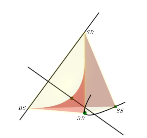
Figure 1: The Spohn variety is a reducible curve of degree four in $\mathbb{P}^{3}$. It has three components but only one passes through the tetrahedron. The figure also shows the Segre surface in the tetrahedron. The curve and the surface meet in one point, namely the totally mixed Nash equilibrium.

The curve in Figure 1 has multiple components because the payoff matrices in (2) are very special. If we perturb the matrix entries, then the resulting curve $\mathcal{V}_{X}$ will be smooth and irreducible in $\mathbb{P}^{3}$. As we shall see, the analogous result holds for games of arbitrary size.

We now present our first result in this section. It summarizes the essential geometric features of Spohn varieties, and it shows how these varieties are related to the Nash equilibria.

Theorem 6.

If the payoff tables $X$ are generic then the Spohn variety $\mathcal{V}_{X}$ is irreducible of codimension $d_{1}+d_{2}+\cdots+d_{n}-n$ and degree $d_{1}d_{2}\ldots d_{n}$. The intersection of $\mathcal{V}_{X}$ with the Segre variety in the open simplex $\Delta$ is precisely the set of totally mixed Nash equilibria for $X$.

Proof.

Consider a generalized column of the $d_{i}\times 2$ matrix $M_{i}$, i.e. a linear combination of the columns of $M_{i}$ with coefficients $\lambda_{1},\lambda_{2}\in\mathbb{R}$ that are not both zero. Since the payoff table $X^{(i)}$ is generic, every generalized column of $M_{i}$ consists of linearly independent linear forms. We know from [8, Theorem 6.4] that the ideal generated by the $2\times 2$ minors of $M_{i}$ is prime of codimension $d_{i}-1$. Moreover, by [5, Proposition 2.15], the degree of this linear determinantal variety is $\binom{2+d_{i}-1-1}{d_{i}-1}=d_{i}$. Since the tensor $X^{(i)}$ is generic and its entries occur only in $M_{i}$, the intersection of the $n$ varieties is transversal. Now, [18, Theorem 1.24] and Bézout’s Theorem for dimensionally transverse intersections yield the first assertion.

The second assertion says that the totally mixed Nash equilibria are the dependency equilibria of rank one. Set $p_{j_{1}\ldots j_{n}}=\pi^{(1)}_{j_{1}}\cdots\pi^{(n)}_{j_{n}}$ with $\pi^{(i)}_{k}>0$ for $k\in[d_{i}]$ and $i\in[n]$. Suppose (1) holds. The dependency equilibria of rank one are defined by the $2\times 2$ minors of the matrix

$$\begin{bmatrix}\,\,\,1\quad&\sum_{j_{1}=1}^{d_{1}}\cdots\widehat{\sum_{j_{i}=1}^{d_{i}}}\cdots\sum_{j_{n}=1}^{d_{n}}X^{(i)}_{j_{1}\cdots 1\cdots j_{n}}\pi^{(1)}_{j_{1}}\cdots\pi^{(i-1)}_{j_{i-1}}\pi^{(i+1)}_{j_{i+1}}\cdots\pi^{(n)}_{j_{n}}\vskip 3.0pt plus 1.0pt minus 1.0pt\\ \,\,\,\vdots\quad&\vdots\\ \,\,\,1\quad&\sum_{j_{1}=1}^{d_{1}}\cdots\widehat{\sum_{j_{i}=1}^{d_{i}}}\cdots\sum_{j_{n}=1}^{d_{n}}X^{(i)}_{j_{1}\cdots d_{i}\cdots j_{n}}\pi^{(1)}_{j_{1}}\cdots\pi^{(i-1)}_{j_{i-1}}\pi^{(i+1)}_{j_{i+1}}\cdots\pi^{(n)}_{j_{n}}\end{bmatrix}\!.$$

We subtract the first row from the $k$th row for all $k\in\{2,\ldots,d_{i}\}$. The $2\times 2$ minors of the resulting matrix are the pairwise differences of the entries in the second column. These differences are precisely the $d_{i}-1$ multilinear equations exhibited in [21, Theorem 6.6]. ∎

The Spohn variety $\mathcal{V}_{X}$ is a high-dimensional projective variety associated with a game $X$. Each point $P$ on $\mathcal{V}_{X}$ is a tensor. We say that $P$ is a Nash point if that tensor has rank one. The positive Nash points in $\mathcal{V}_{X}\cap\Delta$ are the totally mixed Nash equilibria. Their number is given by the formula in [21, Section 6.4], namely it expressed as the mixed volume of certain products of simplices. That mixed volume is zero when the tensor format is too unbalanced.

Remark 7.

A generic game $X$ has no Nash points unless

$$\quad d_{i}\,\,\leq\,\,d_{1}+\cdots+d_{i-1}+d_{i+1}+\cdots+d_{n}-n+2\qquad\hbox{for}\,\,\,\,i=1,2,\ldots,n.$$ (6)

Experts on tensor geometry recognize these inequalities from a result by Gel’fand, Kapranov and Zelevinsky on hyperdeterminants [10, Theorem 14.I.1.3]. Namely, the existence of Nash points for a given tensor format is equivalent to the hyperdeterminant being a hypersurface. In particular, two-person games have Nash points if and only if the matrix is square ($d_{1}=d_{2}$).

We continue to assume that the payoff tables are generic. Then the following result holds.

Theorem 8.

If $n=d_{1}=d_{2}=2$ then the Spohn variety $\mathcal{V}_{X}$ is an elliptic curve. In all other cases, the Spohn variety $\mathcal{V}_{X}$ is rational, represented by a map onto $(\mathbb{P}^{1})^{n}$ with linear fibers.

Proof.

We shall provide a parametrization of $\mathcal{V}_{X}$. Along the way, we shall see why the case $n=d_{1}=d_{2}=2$ is special. The entries of these $n$ matrices $M_{i}$ in (5) are linear forms in the entries $p_{j_{1}\cdots j_{n}}$ of the tensor $P$. Their coefficients depend linearly on the entries of $X$.

Consider the affine line whose coordinate $x_{i}=PX^{(i)}$ is the expected payoff (3) for player $i$. We embed this into a projective line $\mathbb{P}^{1}$ by setting $z_{i}=(x_{i}:-1)$. We call $(\mathbb{P}^{1})^{n}$ the algebraic payoff space. Its homogeneous coordinates are $z=(z_{1},z_{2},\ldots,z_{n})$. The algebraic payoff map is the following rational map from the Spohn variety to the algebraic payoff space:

$$\pi_{X}:\mathcal{V}_{X}\,\dashrightarrow\,(\mathbb{P}^{1})^{n}\,,\,\,P\,\mapsto\,\bigl{(}\,{\rm ker}(M_{1}(P))\,,\,{\rm ker}(M_{2}(P))\,,\,\ldots,\,{\rm ker}(M_{n}(P))\,\bigr{)}.$$ (7)

The name “payoff map” is justified as follows. Suppose that $P$ is a dependency equilibrium, so $P$ is a point in the set $\mathcal{V}_{X}\cap\Delta$. The expected payoff $x_{i}$ for the $i$th player satisfies

$$M_{i}(P)\cdot\begin{bmatrix}\phantom{-}x_{i}\,\\ -1\,\end{bmatrix}\,=\,0\quad{\rm for}\quad i=1,2,\ldots,n.$$ (8)

To see this, augment the rank one matrix $M_{i}(P)$ by its row of column sums, like in (18). Equation (8) implies $\pi_{X}(P)=\bigl{(}(x_{1}\!:\!-1),\ldots,(x_{n}\!:\!-1)\bigr{)}$. We now write (8) on $(\mathbb{P}^{1})^{n}$ as follows:

$$M_{i}(P)\cdot z_{i}^{T}\,=\,K_{X,i}(z_{i})\cdot P,$$ (9)

where the tensor $P$ is vectorized as column. The matrix $K_{X,i}(z_{i})$ has $d_{i}$ rows and $d_{1}d_{2}\cdots d_{n}$ columns. Its entries are binary forms in $z_{i}$ whose coefficients depend on the entries of $X^{(i)}$.

Definition 9.

The Konstanz matrix $K_{X}(z)$ of the game $X$ is a matrix with $\sum_{i=1}^{n}d_{i}$ rows and $d_{1}d_{2}\cdots d_{n}$ columns. It is obtained by stacking the matrices $K_{X,1}(z_{1}),\ldots,K_{X,n}(z_{n})$ on top of each other. When working on the affine chart $z_{i}=(x_{i}:-1)$, we write $K_{X}(x)$.

The Konstanz matrix $K_{X}(z)$ has linearly independent rows when $z$ is generic. Therefore, its kernel is a vector space of dimension $D=\prod_{i=1}^{n}d_{i}-\sum_{i=1}^{n}d_{i}$. We regard ${\rm ker}(K_{X}(z))$ as a linear subspace of dimension $D-1$ in the projective space $\mathbb{P}(V)$. Our construction implies that the Spohn variety is the union of these linear spaces for $z\in(\mathbb{P}^{1})^{n}$:

$$\mathcal{V}_{X}\quad=\quad\bigl{\{}\,P\in\mathbb{P}(V)\,:\,K_{X}(z)\cdot P=0\,\,\,\hbox{for some}\,z\in(\mathbb{P}^{1})^{n}\,\bigr{\}}.$$ (10)

At this point we must distinguish the cases $D\geq 1$ and $D=0$. First, let $D\geq 1$. Then the map $\pi_{X}$ is dominant, and its generic fiber is a linear space $\mathbb{P}^{D-1}$. This map furnishes an explicit birational isomorphism between the Spohn variety $\mathcal{V}_{X}$ and $\mathbb{P}^{D-1}\times(\mathbb{P}^{1})^{n}$. The representation (10) gives the inverse, hence the desired rational parametrization of $\mathcal{V}_{X}$. This confirms the dimension formula in Theorem 6, which is here rewritten as ${\rm dim}(\mathcal{V}_{X})=D-1+n$.

Finally, let $D=0$. This implies $n=d_{1}=d_{2}=2$, so the Konstanz matrix has format $4\times 4$. It is shown in (19). The determinant of $K_{X}(z)$ is a curve of degree $(2,2)$ in $\mathbb{P}^{1}\times\mathbb{P}^{1}$, so it is an elliptic curve. The map $\pi_{X}$ gives a birational isomorphism from $\mathcal{V}_{X}$ onto this curve. This elliptic curve is studied in detail in Section 4, and we will revisit it in Example 16. ∎

The case $D=1$ is also of special interest, because here $\pi_{X}$ is a birational isomorphism.

Example 10 (Del Pezzo surfaces of degree two).

Let $n=2,d_{1}=3,d_{2}=2$. Up to relabelling, this is the only case satisfying $D=1$. The Konstanz matrix equals

$$K_{X}(x)\quad=\quad\begin{bmatrix}\,x_{1}-a_{11}&x_{1}-a_{12}&0&0&0&0\\ 0&0&x_{1}-a_{21}&x_{1}-a_{22}&0&0\\ 0&0&0&0&x_{1}-a_{31}&x_{1}-a_{32}\,\\ \,x_{2}-b_{11}&0&x_{2}-b_{21}&0&x_{2}-b_{31}&0\\ 0&x_{2}-b_{12}&0&x_{2}-b_{22}&0&x_{2}-b_{32}\,\end{bmatrix}.$$ (11)

Here $(x_{1},x_{2})$ are coordinates on an affine chart $\mathbb{C}^{2}$ of $\mathbb{P}^{1}\times\mathbb{P}^{1}$. The rank of (11) drops from $5$ to $4$ at precisely six points in $\mathbb{P}^{1}\times\mathbb{P}^{1}$. Five of these lie in $\mathbb{C}^{2}$. We obtain a rational map

$$\mathbb{P}^{1}\times\mathbb{P}^{1}\dashrightarrow\mathbb{P}^{5}\,,\,(x_{1},x_{2})\mapsto{\rm ker}(K_{X}(x)).$$

This blows up six points, and its image is the Spohn surface $\mathcal{V}_{X}$. The inverse map is $\pi_{X}$. We conclude that $\mathcal{V}_{X}$ is the blow-up of $\mathbb{P}^{1}\times\mathbb{P}^{1}$ at six general points. When seen through the lens of algebraic geometry [7, Example 1.9], this is a del Pezzo surface of degree two. $\diamond$

Konstanz matrices for three other tensor formats are shown in Examples 16, 20 and 21.

4 Elliptic Curves

In this section we take a closer look at $2\times 2$ games, with payoff matrices $X^{(1)}=(a_{ij})$ and $X^{(2)}=(b_{ij})$. The Spohn variety $\mathcal{V}_{X}$ is the elliptic curve in $\mathbb{P}^{3}$ defined by the two quadrics

$$\begin{matrix}\!f_{1}\,=\,{\rm det}(M_{1})\,=(a_{21}-a_{11})p_{11}p_{21}+(a_{22}-a_{11})p_{11}p_{22}+(a_{21}-a_{12})p_{12}p_{21}+(a_{22}-a_{12})p_{12}p_{22},\,\\ f_{2}\,\,=\,{\rm det}(M_{2})\,=(b_{12}-b_{11})p_{11}p_{12}\,+(b_{22}-b_{11})p_{11}p_{22}\,+\,(b_{12}-b_{21})p_{12}p_{21}+\,(b_{22}-b_{21})p_{21}p_{22}.\,\end{matrix}$$

This curve passes through the coordinate points $E_{11},E_{12},E_{21},E_{22}$ in $\mathbb{P}^{3}$. It is smooth and irreducible when $a_{ij}$ and $b_{ij}$ are generic. A planar model of this elliptic curve is obtained by eliminating $p_{22}$ from $f_{1}$ and $f_{2}$. Setting $\,p_{11}=x,\,p_{12}=y,\,p_{21}=z$, we find the ternary cubic

$$\begin{matrix}\quad(a_{11}-a_{22})(b_{11}-b_{12})\,x^{2}y\,+\,(a_{11}-a_{21})(b_{22}-b_{11})\,x^{2}z\,+\,(a_{12}-a_{22})(b_{11}-b_{12})\,xy^{2}\\ +\,(a_{11}-a_{21})(b_{22}-b_{21})\,xz^{2}+\,(a_{12}-a_{22})(b_{21}-b_{12})\,y^{2}z\,+\,(a_{12}-a_{21})(b_{22}-b_{21})\,yz^{2}\\ \qquad\qquad\qquad\qquad\qquad\qquad+\,\bigl{(}\,(a_{12}-a_{21})(b_{22}-b_{11})\,+\,(a_{11}-a_{22})(b_{21}-b_{12})\,\bigr{)}\,xyz.\end{matrix}$$ (12)

A ternary cubic of the form (12) is called a Spohn cubic. This passes through the three coordinate points in $\mathbb{P}^{2}$. But there are other restrictions. To see this, we consider all cubics

$$c_{1}x^{2}y\,+\,c_{2}x^{2}z\,+\,c_{3}xy^{2}\,+\,c_{4}xz^{2}\,+\,c_{5}y^{2}z\,+\,c_{6}yz^{2}\,+\,c_{7}xyz.$$ (13)

The set of such cubics is a projective space $\mathbb{P}^{6}$ with homogeneous coordinates $c_{1},\ldots,c_{7}$.

Proposition 11.

The Spohn cubics (12) form the $4$-dimensional variety in $\mathbb{P}^{6}$ given by $c_{1}+c_{2}-c_{3}-c_{4}+c_{5}+c_{6}-c_{7}=c_{2}c_{4}c_{5}-c_{3}c_{4}c_{5}-c_{2}c_{3}c_{6}+c_{4}c_{5}c_{6}+c_{3}c_{4}c_{7}-c_{4}c_{5}c_{7}-c_{4}^{2}c_{5}+c_{4}c_{5}^{2}=0$. This is a cubic hypersurface inside a hyperplane $\mathbb{P}^{5}$. Its singular locus consists of nine points.

Proof.

This is obtained by a direct computation using the software Macaulay2 [11]. ∎

While the general Spohn cubic is smooth, it can be singular for special payoff matrices. To identify these, we compute the discriminant $\mathcal{D}$ of the ternary cubic (13). This discriminant is an irreducible polynomial of degree $12$ in seven unknowns. It is a sum of $127$ terms:

$$\mathcal{D}\,\,=\,\,16c_{1}^{5}c_{4}^{2}c_{5}^{2}c_{6}^{3}+16c_{1}^{4}c_{2}^{2}c_{5}^{2}c_{6}^{4}-24c_{1}^{4}c_{2}c_{4}^{2}c_{5}^{3}c_{6}^{2}+\,\cdots\,+c_{2}^{2}c_{3}^{2}c_{4}^{2}c_{5}^{2}c_{7}^{4}-c_{2}^{2}c_{3}^{2}c_{4}c_{5}c_{6}c_{7}^{5}.$$

We now plug in the Spohn cubic (12). The resulting discriminant is a polynomial of degree $24$ in the eight unknowns $a_{ij},b_{ij}$. It factors into nine irreducible factors, namely $\,\mathcal{D}(a,b)=$

$$(a_{11}-a_{12})^{2}(a_{11}-a_{21})^{2}(a_{12}-a_{22})^{2}(a_{21}-a_{22})^{2}(b_{11}-b_{12})^{2}(b_{11}-b_{21})^{2}(b_{12}-b_{22})^{2}(b_{21}-b_{22})^{2}\mathcal{E}(a,b).$$

The last factor $\mathcal{E}(a,b)$ has $587$ terms of degree $8$. Nonvanishing of the discriminant $\mathcal{D}(a,b)$ ensures that the Spohn cubic (12) is smooth in $\mathbb{P}^{2}$, and hence so is the curve $\mathcal{V}_{X}$ in $\mathbb{P}^{3}$.

We have argued that the general Spohn curve $\mathcal{V}_{X}$ is an elliptic curve. It is thus natural to express its j-invariant, which identifies the isomorphism type, in terms of the payoff matrices.

Proposition 12.

The j-invariant of the Spohn cubic equals $\,\mathcal{I}(a,b)^{3}/\mathcal{D}(a,b)$, where $\mathcal{I}(a,b)$ is an irreducible polynomial of degree $8$ with $633$ terms in the entries of the two payoff tables.

Proof.

For any ternary cubic, the j-invariant is the cube of the Aronhold invariant divided by the discriminant; see [13, Example 11.12]. Here, $\mathcal{I}(a,b)$ is the Aronhold invariant of (12). ∎

The dependency equilibria of our game are the points in $\mathcal{V}_{X}\cap\Delta$. To better understand this semialgebraic set, we identify some landmarks on the curve $\mathcal{V}_{X}$. The first such landmark is the Nash point, which is the unique rank one matrix in $\mathbb{P}^{3}$ lying on $\mathcal{V}_{X}$:

$$N\,\,=\,\,\begin{bmatrix}b_{22}-b_{21}\\ b_{11}-b_{12}\end{bmatrix}\begin{bmatrix}a_{22}-a_{12}&a_{11}-a_{21}\end{bmatrix}$$ (14)

Suppose that the following holds and the two signs are non-zero:

$${\rm sign}(a_{11}-a_{21})={\rm sign}(a_{22}-a_{12})\quad{\rm and}\quad{\rm sign}(b_{11}-b_{12})={\rm sign}(b_{22}-b_{21}).$$ (15)

Then we can scale the matrix $N$ in (14) by $\bigl{(}(a_{11}-a_{21}+a_{22}-a_{12})(b_{11}-b_{12}+b_{22}-b_{21})\bigr{)}^{-1}$ to land in $\Delta$, and the result is the unique totally mixed Nash equilibrium of the game.

Next recall that the four coordinate points $E_{ij}$ lie on the curve $\mathcal{V}_{X}$. Their tangent lines ${\rm span}(D_{ij},E_{ij})$ are specified by their intersection points with the opposite coordinate planes:

$$\small\begin{matrix}\!D_{11}=\begin{bmatrix}0\!\!&\!\!(a_{11}{-}a_{21})(b_{22}{-}b_{11})\\ (a_{22}{-}a_{11})(b_{11}{-}b_{12})\!\!&\!\!(a_{11}{-}a_{21})(b_{11}{-}b_{12})\end{bmatrix}\!,D_{12}=\begin{bmatrix}(a_{22}{-}a_{12})(b_{12}{-}b_{21})\!\!&\!\!0\\ (a_{22}{-}a_{12})(b_{11}{-}b_{12})\!\!&\!\!(a_{12}{-}a_{21})(b_{11}{-}b_{12})\end{bmatrix}\vskip 6.0pt plus 2.0pt minus 2.0pt\\ \!D_{21}=\begin{bmatrix}(a_{21}{-}a_{12})(b_{21}{-}b_{22})\!\!&\!\!(a_{11}{-}a_{21})(b_{21}{-}b_{22})\\ 0\!\!&\!\!(a_{11}{-}a_{21})(b_{12}{-}b_{21})\end{bmatrix}\!,D_{22}=\begin{bmatrix}(a_{22}{-}a_{12})(b_{21}{-}b_{22})\!\!&\!\!(a_{11}{-}a_{22})(b_{21}{-}b_{22})\\ (a_{12}{-}a_{22})(b_{11}{-}b_{22})\!\!&\!\!0\end{bmatrix}\end{matrix}$$

And, finally, our curve intersects each coordinate plane in a unique non-coordinate point:

$$\small\begin{matrix}\!F_{11}=\begin{bmatrix}0\!\!&\!\!(a_{12}{-}a_{21})(b_{21}{-}b_{22})\\ (a_{12}{-}a_{22})(b_{21}{-}b_{12})\!\!&\!\!(a_{12}{-}a_{21})(b_{12}{-}b_{21})\end{bmatrix}\!,F_{12}=\begin{bmatrix}(a_{11}{-}a_{22})(b_{21}{-}b_{22})\!\!&\!\!0\\ (a_{11}{-}a_{22})(b_{22}{-}b_{11})\!\!&\!\!(a_{11}{-}a_{21})(b_{11}{-}b_{22})\end{bmatrix}\vskip 6.0pt plus 2.0pt minus 2.0pt\\ \!F_{21}=\begin{bmatrix}(a_{12}{-}a_{22})(b_{11}{-}b_{22})\!\!&\!\!(a_{11}{-}a_{22})(b_{22}{-}b_{11})\\ 0\!\!&\!\!(a_{11}{-}a_{22})(b_{11}{-}b_{12})\end{bmatrix}\!,F_{22}=\begin{bmatrix}(a_{12}{-}a_{21})(b_{12}{-}b_{21})\!\!&\!\!(a_{11}{-}a_{21})(b_{21}{-}b_{12})\\ (a_{12}{-}a_{21})(b_{11}{-}b_{12})\!\!&\!\!0\end{bmatrix}\end{matrix}$$

We now show that dependency equilibria may exist even if there are no Nash equilibria in $\Delta$:

Example 13 (Disconnected equilibria).

Consider the game $X$ given by the payoff matrices

$$\begin{bmatrix}a_{11}\!&\!a_{12}\\ a_{21}\!&\!a_{22}\end{bmatrix}=\begin{bmatrix}2&0\\ 4&1\end{bmatrix}\quad{\rm and}\quad\begin{bmatrix}b_{11}\!&\!b_{12}\\ b_{21}\!&\!b_{22}\end{bmatrix}=\begin{bmatrix}2&1\\ 4&3\end{bmatrix},\quad\hbox{with Nash point}\,\,N\,=\,\begin{bmatrix}-1&2\\ \phantom{-}1&\!\!\!-2\end{bmatrix}\!.$$

Here, $\mathcal{V}_{X}$ is smooth and irreducible. This elliptic curve has j-invariant $-(7^{3}103^{3})/(2^{8}3^{2}47)$. The real curve $\mathcal{V}_{X}\cap\Delta$ has two connected components, both disjoint from the Segre surface $\langle p_{11}p_{22}-p_{12}p_{21}\rangle$. One arc connects $E_{11}$ and $F_{21}$, and the other arc connects $E_{22}$ and $F_{12}$. $\diamond$

The combinatorics of the curve $\mathcal{V}_{X}\cap\Delta$ is given by the signs of the entries in the nine matrices $N$, $D_{ij}$ and $F_{ij}$. These signs are determined by the respective orderings of $a_{11},a_{12},a_{21},a_{22}$ and $b_{11},b_{12},b_{21},b_{22}$, assuming that these are quadruples of distinct numbers. We derive the following theorem by analyzing all $(4!)^{2}=576$ possibilities for these pairs of orderings.

Theorem 14.

For a generic $2\times 2$ game $X$, the curve of dependency equilibria $\mathcal{V}_{X}\cap\Delta$ has either $\,0$, $1$ or $2$ connected components, each of which is an arc between two boundary points. If (15) holds then there is exactly one $EE$, $EF$ or $FF$ arc. If (15) does not hold then all components are $EF$ arcs, and their number can be $\,0$, $1$ or $2$.

5 The Payoff Region

The $n$ payoff tensors $X^{(i)}$ define a canonical linear map from tensor space to payoff space:

$$\pi_{X}\,:\,V\rightarrow\mathbb{R}^{n}\,,\,\,\,P\,\,\mapsto\,\,\bigl{(}PX^{(1)},\,PX^{(2)},\,\ldots\,,\,PX^{(n)}\bigr{)}.$$ (16)

The $i$th coordinate $PX^{(i)}$ is the expected payoff for player $i$, given by the formula in (3). We call $\pi_{X}$ the payoff map. By (8), this is the lifting to $V$ of the algebraic payoff map in (7).

The image of the probability simplex $\Delta$ is a convex polytope $\pi_{X}(\Delta)$ that is usually full-dimensional in $\mathbb{R}^{n}$. This polytope is known as the cooperative payoff region of the game $X$. Its points are all possible expected payoff vectors for the game in question. Tu and Jiang [23] investigate the semialgebraic subset that is obtained by projecting all rank one tensors in $\Delta$. This is a nonconvex subset of $\pi_{X}(\Delta)$, known as the noncooperative payoff region.

For $2\times 2$ games, this region is the image of the Segre surface under a linear projection into the plane. Our readers might like to compare [23, Figure 1] with the surface shown in Figure 1.

We are interested in the subset of payoff vectors that arise from dependency equilibria:

$$\mathcal{P}_{X}\,:=\,\pi_{X}(\mathcal{V}_{X}\cap\Delta)\,\subset\,\pi_{X}(\Delta)\,\subset\,\mathbb{R}^{n}.$$

The set $\mathcal{P}_{X}$ is semialgebraic, by Tarski’s Theorem on Quantifier Elimination. The authors of [23] would probably call $\mathcal{P}_{X}$ the dependency payoff region of the game $X$. In the present paper, we just use the term payoff region for $\mathcal{P}_{X}$, since our focus is on dependency equilibria.

We begin by noting that, at every dependency equilibrium of $X$, the expected payoffs agree with the various conditional expected payoffs. We can thus use conditional expectations in (16) to define the payoff region $\mathcal{P}_{X}$. This is the content of the following lemma.

Lemma 15.

Let $P$ be a tensor in $V$ with $p_{++\cdots+}=1$ that represents a point in $\mathcal{V}_{X}$. Then

$$PX^{(i)}\,\,=\,\,\sum_{j_{1}=1}^{d_{1}}\cdots\widehat{\sum_{j_{i}=1}^{d_{i}}}\cdots\sum_{j_{n}=1}^{d_{n}}X^{(i)}_{j_{1}\cdots k\cdots j_{n}}\frac{p_{j_{1}\cdots k\cdots j_{n}}}{p_{+\cdots+k+\cdots+}}\quad\hbox{for all $\,i\in[n]\,$ and $\,k\in[d_{i}]$.}$$ (17)

Proof.

The $d_{i}\times 2$ matrix $M_{i}$ in (5) has rank one, by definition of $\mathcal{V}_{X}$. We replace the first row by the sum of all rows. This transforms $M_{i}$ into the following matrix whose rank is one:

$$\small\begin{bmatrix}\,1&PX^{(i)}\\ \,p_{+\cdots+2+\cdots+}&\sum_{j_{1}=1}^{d_{1}}\cdots\widehat{\sum_{j_{i}=1}^{d_{i}}}\cdots\sum_{j_{n}=1}^{d_{n}}X^{(i)}_{j_{1}\cdots 2\cdots j_{n}}p_{j_{1}\cdots 2\cdots j_{n}}\\ \,\vdots&\vdots\\ \,p_{+\cdots+d_{i}+\cdots+}&\sum_{j_{1}=1}^{d_{1}}\cdots\widehat{\sum_{j_{i}=1}^{d_{i}}}\cdots\sum_{j_{n}=1}^{d_{n}}X^{(i)}_{j_{1}\cdots d_{i}\cdots j_{n}}p_{j_{1}\cdots d_{i}\cdots j_{n}}\end{bmatrix}\!.$$ (18)

The $2\times 2$ minor given by the first row and the $k$th row is zero; see also (8). This implies the desired identity (17) for $k\geq 2$. The case $k=1$ is obtained by swapping rows in $M_{i}$. ∎

Example 16 ($2\times 2$ games).

The polygon $\pi_{X}(\Delta)$ is the convex hull in $\mathbb{R}^{2}$ of the points $(a_{11},b_{11})$, $(a_{12},b_{12})$, $(a_{21},b_{21})$ and $(a_{22},b_{22})$, so it is typically a triangle or a quadrilateral. This polygon contains the payoff curve $\mathcal{P}_{X}$, which is the image of the curve $\mathcal{V}_{X}\cap\Delta$ under the payoff map $\pi_{X}$. This is a plane cubic, defined by the determinant of the Konstanz matrix

$$K_{X}(x)\quad=\quad\begin{bmatrix}x_{1}-a_{11}&x_{1}-a_{12}&0&0\\ 0&0&x_{1}-a_{21}&x_{1}-a_{22}\\ x_{2}-b_{11}&0&x_{2}-b_{21}&0\\ 0&x_{2}-b_{12}&0&x_{2}-b_{22}\end{bmatrix}.$$ (19)

For each point $x$ on this curve, the kernel of (19) gives the unique matrix $P$ satisfying $\pi_{X}(P)=x$. The payoff region $\mathcal{P}_{X}$ is the subset of points $x$ on the curve for which $P>0$.

Figure 2(a) shows the payoff region for the Bach or Stravinsky game in Example 1. It is the blue arc inside the yellow triangle $\pi_{X}(\Delta)={\rm conv}\{(0,0),(2,3),(3,2)\}$. This picture is the image of Figure 1 under the payoff map $\pi_{X}$. Figure 2(b) shows a perturbed version, with $a_{11}=3.3$ and $b_{22}=3.2$, where the Spohn curve is irreducible. $\diamond$

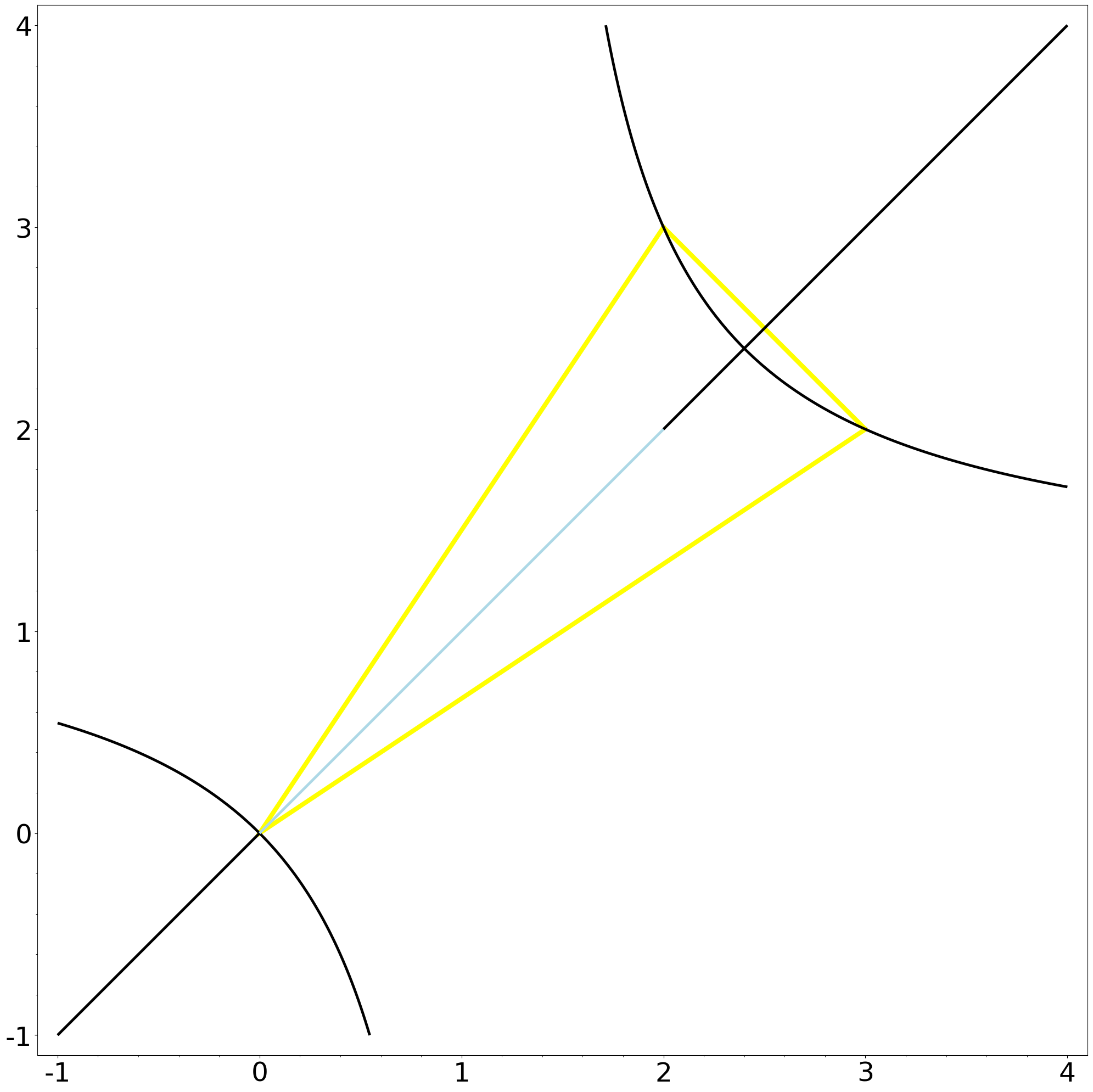
(a)

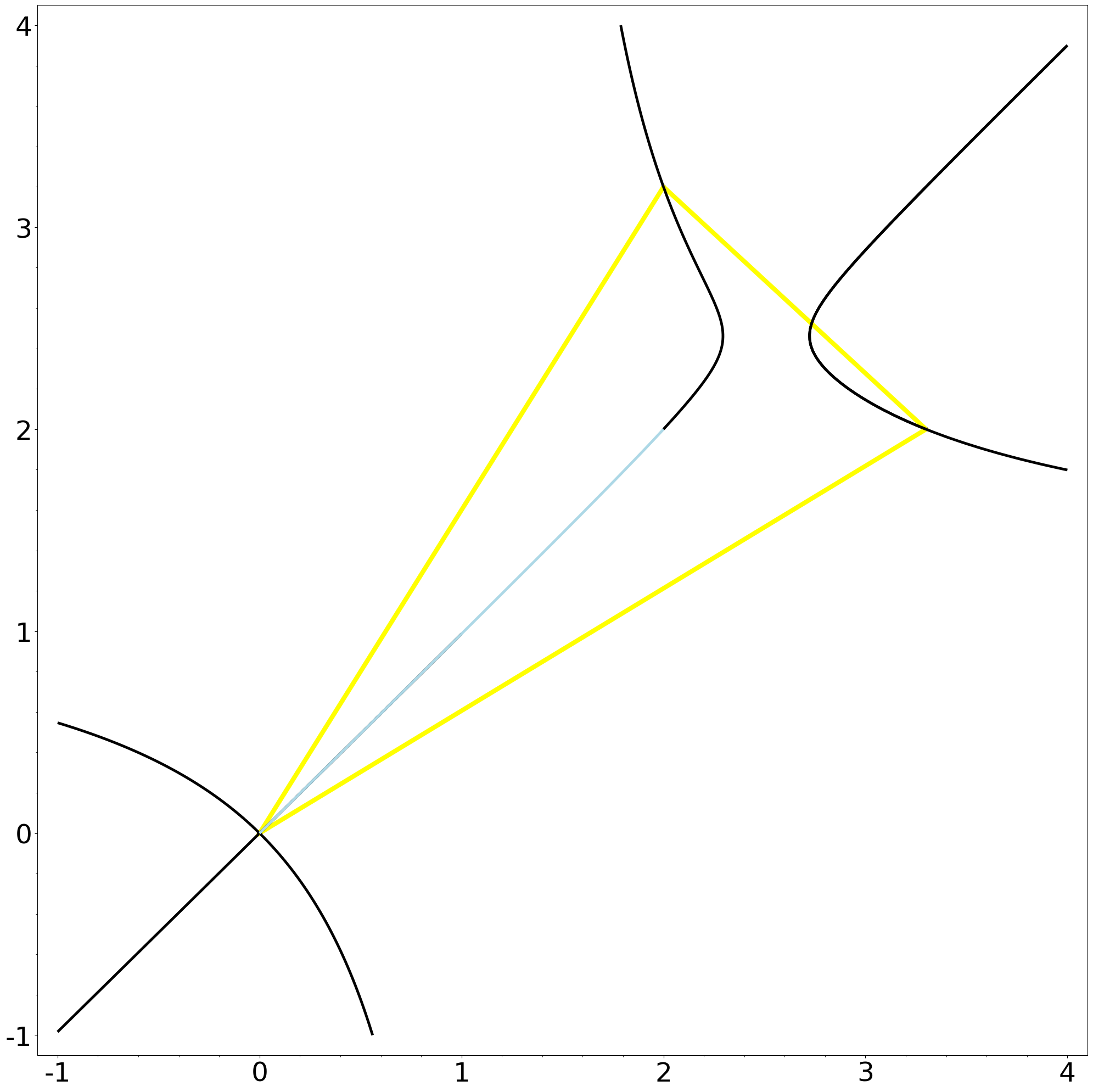
(b)

Figure 2: The payoff region for each of these $2\times 2$ games is the blue arc in the yellow triangle.

We now consider cases other than $2\times 2$ games, so that ${\rm dim}(\mathcal{V}_{X})\geq n$ holds. We further assume that $X$ is generic and that $\mathcal{V}_{X}\cap\Delta$ is non-empty. Since the algebraic payoff map $\pi_{X}$ in (7) is dominant, the payoff region $\mathcal{P}_{X}$ is a full-dimensional semialgebraic subset of $\mathbb{R}^{n}$.

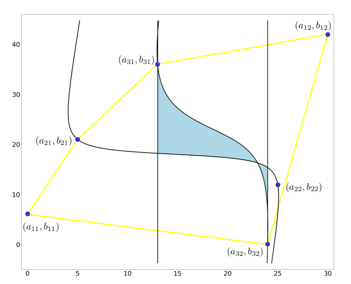
Figure 3: The payoff region $\mathcal{P}_{X}$ for the $3\times 2$ game in Example 17 consists of two curvy triangles, inside the pentagon $\pi_{X}(\Delta)$. Its boundary is given by two lines and two cubics.

Example 17 ($3\times 2$ games).

The following two payoff matrices exhibit the generic behavior:

$$\small X^{(1)}\,=\,\begin{bmatrix}a_{11}&\!a_{12}\\ a_{21}&\!a_{22}\\ a_{31}&\!a_{32}\end{bmatrix}\,=\,\begin{bmatrix}0&30\\ 5&25\\ 13&24\end{bmatrix}\quad{\rm and}\quad\,\,X^{(2)}\,=\,\begin{bmatrix}b_{11}&\!b_{12}\\ b_{21}&\!b_{22}\\ b_{31}&\!b_{32}\end{bmatrix}\,=\,\begin{bmatrix}6&42\\ 21&12\\ 36&0\end{bmatrix}.$$ (20)

The polygon $\pi_{X}(\Delta)$ is the pentagon whose vertices are $(a_{ij},b_{ij})$ with $\{i,j\}\neq\{2,2\}$. The payoff region $\mathcal{P}_{X}=\pi_{X}(\mathcal{V}_{X}\cap\Delta)$ is shaded in blue in Figure 3. The algebraic boundary of $\mathcal{P}_{X}$ is given by the two cubics $9x_{1}^{2}x_{2}-2x_{1}x_{2}^{2}-162x_{1}^{2}-189x_{1}x_{2}+30x_{2}^{2}+3906x_{1}-540x_{2}+2160$ and $72x_{1}^{2}x_{2}-19x_{1}x_{2}^{2}-1512x_{1}^{2}-1614x_{1}x_{2}+390x_{2}^{2}+36288x_{1}-2340x_{2}$, plus the two vertical lines $x_{1}-13$ and $x_{1}-24$. The two curvy triangles that form $\mathcal{P}_{X}$ meet at the special point

$$\bigl{(}22.9902299164,16.2987107576\bigr{)}.$$ (21)

Figure 3 illustrates the general behavior for $3\times 2$ games. We can understand this via the del Pezzo geometry in Example 10. The Spohn surface $\mathcal{V}_{X}$ is the blow-up of $\mathbb{P}^{1}\times\mathbb{P}^{1}$ at six points. One of these six is the special point (21). The Konstanz matrix $K_{X}(x)$ in (11) has rank four at this point, so there is a line segment in $\mathcal{V}_{X}\cap\Delta$ that maps to (21) under $\pi_{X}$. At all nearby points $x\in\mathbb{R}^{2}$, the rank of $K_{X}(x)$ is five. Here, $\pi_{X}$ gives a bijection between $\mathcal{V}_{X}\cap\Delta$ and the payoff region $\mathcal{P}_{X}$. The boundary curves of $\mathcal{P}_{X}$ are defined by maximal minors of $K_{X}(x)$. Each minor is a $5\times 5$-determinant, but it has degree four as a polynomial in $x=(x_{1},x_{2})$. That quartic factors into a linear factor $x_{1}-a_{ij}$ times a cubic in $(x_{1},x_{2})$. $\diamond$

We now work towards the main result of this section, generalizing Example 17 to arbitrary tensor formats. The key players are the maximal minors of the Konstanz matrix $K_{X}(x)$.

Lemma 18.

Given any game $X$, each of the $\binom{d_{1}d_{2}\cdots d_{n}}{\,d_{1}+d_{2}+\cdots+d_{n}\,}$ maximal minors of the Konstanz matrix $K_{X}(x)$ is a polynomial of degree at most $\sum_{i=1}^{n}d_{i}-n+1$ in the unknowns $x_{1},\ldots,x_{n}$.

Proof.

The highest degree seen in the maximal minors is the rank of $K_{X}(x)$ after setting all entries in the payoff tables $X^{(i)}$ to zero. After rescaling the rows, the columns of this matrix are homogeneous coordinates for the vertices of the product of standard simplices $\Delta_{d_{1}-1}\times\cdots\times\Delta_{d_{n}-1}$. The dimension of this polytope is one less than the matrix rank. ∎

Suppose now that $X$ is fixed and generic. We consider the stratification of the payoff space $\mathbb{R}^{n}$ defined by the signs taken on by the maximal minors of $K_{X}(x)$. We call this the oriented matroid stratification of the game $X$. Indeed, it is the restriction to $\mathbb{R}^{n}$ of the usual oriented matroid stratification (cf. [14]) of the space of matrices with $\sum_{i=1}^{n}d_{i}$ rows and $\prod_{i=1}^{n}d_{i}$ columns. The maximal minors of $K_{X}(x)$ that are nonzero polynomials give the bases of a matroid. The full-dimensional strata correspond to orientations of that matroid. The open stratum containing a given point $x\in\mathbb{R}^{n}$ consists of all points $x^{\prime}\in\mathbb{R}^{n}$ such that corresponding nonzero maximal minors of $K_{X}(x)$ and $K_{X}(x^{\prime})$ have the same sign $+1$ or $-1$.

The oriented matroid strata in $\mathbb{R}^{n}$ are semialgebraic. Their boundaries are delineated by the maximal minors of $K_{X}(x)$. These minors are the polynomials in Lemma 18. The oriented matroid strata can be disconnected (cf. [14]). This happens in Examples 13 and 17. Note that the union of the two open curvy triangles in Figure 3 is a single chamber (open stratum) for the game $X$ given in (20). It is given by prescribing a fixed sign $+1$ or $-1$ for each of the six maximal minors of (11). Interestingly, $\mathcal{P}_{X}$ itself is connected in this case. The point (21) lies in $\mathcal{P}_{X}$ because its fiber under $\pi_{X}$ is a line that meets the interior of $\Delta$.

We now present our characterization of the payoff region $\mathcal{P}_{X}$ of a generic game $X$. By the algebraic boundary of $\mathcal{P}_{X}$ we mean the Zariski closure of its topological boundary.

Theorem 19.

The payoff region $\mathcal{P}_{X}$ for a generic game $X$ is a union of oriented matroid strata in $\mathbb{R}^{n}$ that are given by the signs of the maximal minors of the Konstanz matrix $K_{X}(x)$. Its algebraic boundary is a union of irreducible hypersurfaces of degree at most $\,\sum_{i=1}^{n}d_{i}-n+1$.

Proof.

For fixed $x\in\mathbb{R}^{n}$, the set of probability tensors $P$ with expected payoffs $x$ is equal to

$${\rm kernel}\bigl{(}K_{X}(x)\bigr{)}\,\,\cap\,\,\Delta.$$ (22)

This is a convex polytope which is either empty or has the full dimension $\prod_{i=1}^{n}d_{i}-\sum_{i=1}^{n}d_{i}-1$. The payoff region $\mathcal{P}_{X}$ is the set of all $x\in\mathbb{R}^{n}$ such that this polytope is nonempty. We know from oriented matroid theory [2, Chapter 9] that the combinatorial type of the polytope (22) is determined by the oriented matroid of the matrix $K_{X}(x)$. Therefore, the combinatorial type is constant as $x$ ranges over a fixed oriented matroid stratum in $\mathbb{R}^{n}$. In particular, whether or not (22) is empty depends only on the oriented matroid of $K_{X}(x)$. Namely, it is non-empty if and only if every column index lies in a positive covector of that oriented matroid. This proves the first sentence. The second sentence follows from Lemma 18. ∎

One of the reasons for our interest in the algebraic boundary is that it helps in characterizing dependency equilibria $P$ that are Pareto optimal. We thus address a question raised in [20, Section 4]. Recall that $P$ is Pareto optimal if its image $x=\pi_{X}(P)$ in $\mathcal{P}_{X}$ satisfies $\,(x+\mathbb{R}^{n}_{\geq 0})\,\cap\,\overline{\mathcal{P}_{X}}=\{x\}$. This condition implies that $x$ lies in the boundary of $\mathcal{P}_{X}$, hence one of the maximal minors of $K_{X}(x)$ must vanish. For instance, for the $3\times 2$ game in Example 17, the Pareto optimal equilibria correspond to the points on the upper-right boundaries of the two curvy triangles in Figure 3. At such points $x$, the product of our two cubics vanishes.

We close this section by discussing Theorem 19 for two cases larger than Example 17.

Example 20 ($3\times 3$ games).

Let $n=2$ and $d_{1}=d_{2}=3$. The Konstanz matrix equals

$$K_{X}(x)\,=\,\small\begin{bmatrix}x_{1}\!-\!a_{11}&\!x_{1}\!-\!a_{12}\!&\!x_{1}\!-\!a_{13}\!&0&0&0&0&0&0\\ 0&0&0&x_{1}\!-\!a_{21}&\!x_{1}\!-\!a_{22}\!&\!x_{1}\!-\!a_{23}\!&0&0&0\\ 0&0&0&0&0&0&\!x_{1}\!-\!a_{31}\!&\!x_{1}\!-\!a_{32}\!&\!x_{1}\!-\!a_{33}\\ x_{2}\!-\!b_{11}&0&0&\!x_{2}\!-\!b_{21}&0&0&\!x_{2}\!-\!b_{31}&0&0\\ 0&\!x_{2}\!-\!b_{12}\!&0&0&\!x_{2}\!-\!b_{22}\!&0&0&\!x_{2}\!-\!b_{32}\!&0\\ 0&0&\!x_{2}\!-\!b_{13}\!&0&0&\!x_{2}\!-\!b_{23}&0&0&\!x_{2}\!-\!b_{33}\end{bmatrix}\!.$$

Among the $\binom{9}{6}=84$ maximal minors of this $6\times 9$ matrix, six are identically zero. Six others are irreducible polynomials of degree five in $x=(x_{1},x_{2})$. Each of the remaining $72$ minors is an irreducible cubic times a product $(x_{1}-a_{ij})(x_{2}-b_{kl})$. The resulting arrangement of lines, cubics and quintics divides the plane $\mathbb{R}^{2}$ into open chambers. We examine the chambers that lie inside the polygon $\pi_{X}(\Delta)$. The rank $6$ oriented matroid of $K_{X}(x)$, given by $78$ signed bases, is constant on each chamber. The payoff region is a union of some of them. $\diamond$

Example 21 ($2\times 2\times 2$ games).

The game played by Adam, Bob and Carl in Example 3 has

$$K_{X}(x)\,=\,\small\begin{bmatrix}x_{1}\!-\!a_{111}&x_{1}\!-\!a_{112}&x_{1}\!-\!a_{121}&x_{1}\!-\!a_{122}&0&0&0&0\\ 0&0&0&0&x_{1}\!-\!a_{211}&x_{1}\!-\!a_{212}&x_{1}\!-\!a_{221}&x_{1}\!-\!a_{222}\\ x_{2}\!-\!b_{111}&x_{2}\!-\!b_{112}&0&0&x_{2}\!-\!b_{211}&x_{2}\!-\!b_{212}&0&0\\ 0&0&x_{2}\!-\!b_{121}&x_{2}\!-\!b_{122}&0&0&x_{2}\!-\!b_{221}&x_{2}\!-\!b_{222}\\ x_{3}\!-\!c_{111}&0&x_{3}\!-\!c_{121}&0&x_{3}\!-\!c_{211}&0&x_{3}\!-\!c_{221}&0\\ 0&x_{3}\!-\!c_{112}&0&x_{3}\!-\!c_{122}&0&x_{3}\!-\!c_{212}&0&x_{3}\!-\!c_{222}\end{bmatrix}\!.$$

All $\binom{8}{6}=28$ maximal minors are irreducible polynomials of degree four in $x=(x_{1},x_{2},x_{3})$. Each of them defines a smooth quartic surface in $\mathbb{C}^{3}$ that has three isolated singularities at infinity in $\mathbb{P}^{3}$. This data specifies an arrangement of $28$ K3 surfaces in $\mathbb{P}^{3}$. We examine its chambers inside the polytope $\pi_{X}(\Delta)$, which has $\leq 8$ vertices. The payoff region $\mathcal{P}_{X}$ is the union of a subset of these chambers, so its algebraic boundary consists of quartic surfaces. $\diamond$

6 Conditional Independence and Bayesian Networks

One drawback of dependency equilibria is that they are abundant. Indeed, if the Spohn variety $\mathcal{V}_{X}$ intersects the open simplex $\Delta$, then the semialgebraic set $\mathcal{V}_{X}\cap\Delta$ of all dependency equilibria has dimension $\prod_{i=1}^{n}d_{i}-\sum_{j=1}^{n}d_{j}+n-1$. This follows from Theorem 6. To mitigate this drawback, we restrict to intersections of $\mathcal{V}_{X}$ with statistical models in $\Delta$. Natural candidates are the conditional independence models in [21, Section 8.1] and [22, Section 4.1].

We view the $n$ players as random variables with state spaces $[d_{1}],\ldots,[d_{n}]$. A point $P$ in $\Delta$ is a joint probability distribution. Let $\mathcal{C}$ be any collection of conditional independence (CI) statements on $[n]$. These statements have the form $A\!\perp\!\!\!\perp\!B\,|\,C$, where $A,B,C$ are pairwise disjoint subsets of $[n]$. Each CI statement translates into a system of homogeneous quadratic constraints in the tensor entries $p_{j_{1}j_{2}\cdots j_{n}}$. This translation is explained in [21, Proposition 8.1] and [22, Proposition 4.1.6]. We write $\mathcal{M}_{\mathcal{C}}$ for the projective variety in $\mathbb{P}(V)$ that is defined by these quadrics, arising from all statements $\,A\!\perp\!\!\!\perp\!B\,|\,C\,$ in $\mathcal{C}$. Here we assume that components lying in the hyperplanes $\{p_{j_{1}j_{2}\cdots j_{n}}=0\}$ and $\{p_{++\cdots+}=0\}$ have been removed.

Suppose $X$ is any game in normal form, and $\mathcal{C}$ is any collection of CI statements. We define the Spohn CI variety to be the intersection of the Spohn variety with the CI model:

$$\mathcal{V}_{X,\mathcal{C}}\,\,=\,\,\mathcal{V}_{X}\,\cap\,\mathcal{M}_{\mathcal{C}}.$$ (23)

We again assume that components lying in the special hyperplanes above have been removed. The intersection $\,\mathcal{V}_{X,\mathcal{C}}\,\cap\,\Delta\,$ with the simplex $\Delta$ is the set of all CI equilibria of the game $X$. This is a semialgebraic set which is a natural extension of the set of Nash equilibria of $X$. In what follows we assume that all random variables are binary, i.e. $d_{1}=d_{2}=\cdots=d_{n}=2$.

Example 22 (Nash points).

Let $\mathcal{C}$ be the set of all CI statements on $[n]$. The model $\mathcal{M}_{\mathcal{C}}$ is the Segre variety of rank one tensors, and the Spohn CI variety (23) is the set of all Nash points in the Spohn variety $\mathcal{V}_{X}$. By [21, Corollary 6.9], this variety is finite, and its cardinality is the number of derangements of $[n]$, which is $1,2,9,44,265,\ldots$ for $n=1,2,3,4,5,\ldots$.

For $n\geq 3$, the Nash points span a linear subspace of codimension $2n$ in $\mathbb{P}(V)\simeq\mathbb{P}^{2^{n}-1}$. To see this, we note that the $i$th multilinear equation in [21, Theorem 6.6] has degree $n-1$ and it misses the $i$th unknown $\pi^{(i)}$. Multiplying that equation by $\pi^{(i)}$ and by $1-\pi^{(i)}$ gives two linear constraints on $\mathbb{P}(V)$ for each $i$. These $2n$ linear forms are linearly independent. $\diamond$

Example 23 ($n=3,d_{1}=d_{2}=d_{3}=2$).

Consider games $X$ for three players with binary choices. The Spohn variety $\mathcal{V}_{X}$ is a complete intersection of dimension $4$ and degree $8$ in $\mathbb{P}^{7}$. It is defined by imposing rank one constraints on the three matrices $M_{i}$ in Example 3. It is parametrized by the lines ${\rm ker}(K_{X}(x))$ where $x\in\mathbb{C}^{3}$ and $K_{X}(x)$ is the matrix in Example 21.

We examine the Spohn CI varieties given by three models $\mathcal{M}_{\mathcal{C}}$ in [21, Section 8.1]. In each case, the intersection (23) is transversal in $\Delta$, and we find that $\mathcal{V}_{X,\mathcal{C}}$ is irreducible in $\mathbb{P}^{7}$.

• Let $\mathcal{C}=\{\,1\!\perp\!\!\!\perp\!2\,|\,3\}$ as in [21, eqn (8.3)]. The CI model $\mathcal{M}_{\mathcal{C}}$ has codimension $2$ and degree $4$, and the Spohn CI variety $\mathcal{V}_{X,\mathcal{C}}$ is a surface of degree $28$ in $\mathbb{P}^{7}$. We find that the prime ideal of $\mathcal{V}_{X,\mathcal{C}}$ is minimally generated by five quadrics and three quartics.

• Let $\mathcal{C}=\{\,2\!\perp\!\!\!\perp\!3\,\}$ as in [21, eqn (8.4)], so here $C=\emptyset$. The CI model $\mathcal{M}_{\mathcal{C}}$ is the hypersurface, defined by the quadric $p_{+11}p_{+22}-p_{+12}p_{+21}$. The Spohn CI variety $\mathcal{V}_{X,\mathcal{C}}$ is a threefold of degree $10$ in $\mathbb{P}^{7}$. Its prime ideal is minimally generated by six quadrics.

• Let $\mathcal{C}=\{\,1\!\perp\!\!\!\perp\!23\,\}$ as in [21, eqn (8.5)]. Here $\mathcal{M}_{\mathcal{C}}\simeq\mathbb{P}^{1}\times\mathbb{P}^{3}$ is defined by the $2\times 2$ minors of a $2\times 4$ matrix obtained by flattening the tensor $P$. The Spohn CI variety $\mathcal{V}_{X,\mathcal{C}}$ is a curve of degree $8$ and genus $3$. It lies in a $\mathbb{P}^{5}$ inside $\mathbb{P}^{7}$. Its prime ideal is generated by two linear forms and seven quadrics. These will be explained after Example 26.

The computation of the prime ideals is non-trivial. One starts with the ideal generated by the natural quadrics defining (23), and one then saturates that ideal by $\,p_{+++}\cdot\prod_{i,j,k=1}^{2}p_{ijk}$. We performed these computations with the computer algebra system Macaulay2 [11]. $\diamond$

Of special interest are graphical models, such as Markov random fields and Bayesian networks. These allow us to describe the nature of the desired equilibria by means of a graph whose nodes are the $n$ players. This is different from the setting of graphical games in [21, Section 6.5], where the graph structure imposes zero patterns in the payoff tables $X^{(i)}$.

Inspired by [19, Section 3], we now focus on Bayesian networks, where the CI statements $\mathcal{C}$ describe the global Markov property of an acyclic directed graph with vertex set $[n]$. These CI statements and their ideals are explained in [9, Section 3]. In Macaulay2, they can be computed using the commands globalMarkov and conditionalIndependenceIdeal in the GraphicalModels package. Sometimes, it is preferable to work with the prime ideal ${\rm ker}(\Phi)$ in [9, Theorem 8]. From this we obtain the ideal of the Spohn CI variety $\mathcal{V}_{X,\mathcal{C}}$ by saturation, as described at the end of Example 23. For all the models we were able to compute, this ideal turned out to be of the expected codimension. In each case, except for the network with no edges, the variety $\mathcal{V}_{X,\mathcal{C}}$ is irreducible. We conjecture that these facts hold in general.

Conjecture 24.

For every Bayesian network $\mathcal{C}$ on $n$ binary random variables, the Spohn CI variety $\,\mathcal{V}_{X,\mathcal{C}}\,$ has the expected codimension $n$ inside the model $\mathcal{M}_{\mathcal{C}}$ in $\mathbb{P}^{2^{n}-1}$. The variety $\mathcal{V}_{X,\mathcal{C}}$ is positive-dimensional and irreducible whenever the network has at least one edge.

Proposition 25.

Conjecture 24 holds for $n\leq 3$.

Proof.

For the network with no edges, $\mathcal{M}_{\mathcal{C}}$ is the Segre variety $(\mathbb{P}^{1})^{n}$. The dimension statement holds, but the Spohn CI variety is reducible, as seen in Example 22. We thus examine all Bayesian networks with at least one edge. These satisfy ${\rm dim}(\mathcal{M}_{\mathcal{C}})\geq n+1$. The case $n\leq 2$ being trivial, we assume that $n=3$. If the network is a complete directed acylic graph, then the ideal of $\mathcal{M}_{\mathcal{C}}$ is the zero ideal and $\mathcal{V}_{X,\mathcal{C}}=\mathcal{V}_{X}$. There are four networks left to be considered. By [9, Proposition 5], they are precisely the three models in Example 23:

(a) $$\,\,1\leftarrow 3\rightarrow 2\,\, \,\,2\rightarrow 3\rightarrow 1 \,\,3\rightarrow 1\leftarrow 2 \,\,3\rightarrow 2\quad 1$$ or    (b)    (c) .

This means that the proof was already given by our analysis in Example 23. ∎

Consider the next case $n=4$. Up to relabeling, there are $29$ Bayesian networks $\mathcal{C}$ with at least one edge. They are listed in [9, Theorem 11], along with a detailed analysis of the variety $\mathcal{M}_{\mathcal{C}}$ in each case. We embarked towards a proof of Conjecture 24, by examining all $29$ models. But the computations are quite challenging, and we leave them for the future.

Example 26.

Consider the network #15 in [9, Table 1]. The variety $\mathcal{M}_{\mathcal{C}}$ has dimension $9$ and degree $48$. An explicit parametrization $\phi$ is shown in [21, page 109]. We can represent $\mathcal{V}_{X,\mathcal{C}}$ by substituting this parametrization into the equations ${\rm det}(M_{i})=0$ for $i=1,2,3,4$. $\diamond$

The smallest irreducible variety in Conjecture 24 arises from the Bayesian network $\mathcal{C}$ with only one edge, here taken to be $n\rightarrow n-1$. The Spohn CI variety $\mathcal{V}_{X,\mathcal{C}}$ contains all the Nash points in Example 22. The rest of this paper is dedicated to this scenario. It is important for applications of dependency equilibria because of its proximity to Nash equilibria.

For our one-edge network, $\mathcal{M}_{\mathcal{C}}$ is the Segre variety $(\mathbb{P}^{1})^{n-2}\times\mathbb{P}^{3}$ embedded into $\mathbb{P}^{2^{n}-1}$. Hence $\mathcal{M}_{\mathcal{C}}$ has dimension $n+1$. The Spohn CI variety $\mathcal{V}_{X,\mathcal{C}}$ is a curve. This curve lies in a linear subspace of codimension $2n-4$ in $\mathbb{P}^{2^{n}-1}$. In addition to the quadrics that define the Segre variety $\mathcal{M}_{\mathcal{C}}$, the ideal of $\mathcal{V}_{X,\mathcal{C}}$ contains $2n-4$ linear forms and $2^{n-1}$ quadrics that depend on the game $X$. The determinants of the matrices $M_{1},M_{2},\ldots,M_{n-2}$ give rise to two linear forms each. The determinants of the matrices $M_{n-1}$ or $M_{n}$ give rise to $2^{n-2}$ quadrics.

For example, if $n=3$ then the variety $\mathcal{M}_{\mathcal{C}}\simeq\mathbb{P}^{1}\times\mathbb{P}^{3}$ has the parametric representation

$$p_{ijk}\,\,=\,\,\sigma_{i}\tau_{jk}\quad\hbox{for}\,\,\,1\leq i,j,k\leq 2.$$

The prime ideal of $\mathcal{M}_{\mathcal{C}}$ is generated by the six $2\times 2$ minors of the matrix

$$\begin{bmatrix}\,p_{111}&p_{112}&p_{121}&p_{122}\\ \,p_{211}&p_{212}&p_{221}&p_{222}\end{bmatrix}.$$ (24)

After removing common factors from rows and columns, the three matrices in Example 3 are

$$M_{1}\,=\,\begin{bmatrix}\,\,\,1\,&\,\,a_{111}\tau_{11}+a_{112}\tau_{12}+a_{121}\tau_{21}+a_{122}\tau_{22}\\ \,\,\,1\,&\,\,a_{211}\tau_{11}+a_{212}\tau_{12}+a_{221}\tau_{21}+a_{222}\tau_{22}\end{bmatrix},$$

$$M_{2}\,=\,\begin{bmatrix}\,\tau_{11}+\tau_{12}&\,b_{111}\sigma_{1}\tau_{11}+b_{112}\sigma_{1}\tau_{12}+b_{211}\sigma_{2}\tau_{11}+b_{212}\sigma_{2}\tau_{12}\\ \,\tau_{21}+\tau_{22}&\,b_{121}\sigma_{1}\tau_{21}+b_{122}\sigma_{1}\tau_{22}+b_{221}\sigma_{2}\tau_{21}+b_{222}\sigma_{2}\tau_{22}\end{bmatrix},$$

$$M_{3}\,=\,\begin{bmatrix}\,\tau_{11}+\tau_{21}&\,c_{111}\sigma_{1}\tau_{11}+c_{121}\sigma_{1}\tau_{21}+c_{211}\sigma_{2}\tau_{11}+c_{221}\sigma_{2}\tau_{21}\\ \,\tau_{12}+\tau_{22}&\,c_{112}\sigma_{1}\tau_{12}+c_{122}\sigma_{1}\tau_{22}+c_{212}\sigma_{2}\tau_{12}+c_{222}\sigma_{2}\tau_{22}\end{bmatrix}.$$

By multiplying ${\rm det}(M_{1})$ with $\sigma_{1}$ and with $\sigma_{2}$, we obtain two linear forms in $p_{111},p_{112},\ldots,p_{222}$ that vanish on $\mathcal{V}_{X}$. Likewise, by multiplying ${\rm det}(M_{2})$ and ${\rm det}(M_{3})$ with $\sigma_{1}$ and with $\sigma_{2}$, we obtain four quadratic forms in $p_{111},p_{112},\ldots,p_{222}$ that vanish on $\mathcal{V}_{X}$. Three of the six minors of (24) are linearly independent modulo the linear forms. This explains the $2+7$ generators of the prime ideal of the curve $\mathcal{V}_{X,\mathcal{C}}$, which has genus $3$ and degree $8$ in $\mathbb{P}^{5}\subset\mathbb{P}^{7}$.

Let now $n=4$. The one-edge model $\mathcal{M}_{\mathcal{C}}$ is the Segre variety $\mathbb{P}^{1}\times\mathbb{P}^{1}\times\mathbb{P}^{3}$ in $\mathbb{P}^{15}$. Its prime ideal is generated by $46$ binomial quadrics. Of these, $32$ are linearly independent modulo the four linear forms that arise from the matrices $M_{1}$ and $M_{2}$ as above. Similarly, $M_{3}$ and $M_{4}$ contribute eight quadrics. We conclude that $\mathcal{V}_{X,\mathcal{C}}$ is an curve of genus $23$ and degree $30$ in $\mathbb{P}^{11}\subset\mathbb{P}^{15}$, and its prime ideal is minimally generated by $4$ linear forms and $40$ quadrics.

In the recent work [16] it is proven, for generic games, that the Spohn CI curve for the one-edge model is an irreducible complete intersection curve in the Segre variety $(\mathbb{P}^{1})^{n-2}\times\mathbb{P}^{3}$. Moreover the authors give an explicit formula for its degree and genus. In the spirit of Datta’s universality theorem for Nash equilibria, they show that any affine real algebraic variety $S\subseteq\mathbb{R}^{m}$ defined by $k$ polynomials with $k<m$ can be represented as the Spohn CI variety of an $n$-person game for one-edge Bayesian networks on $n$ binary random variables.

Acknowledgements

Both authors visited Konstanz in November 2021. The ideas we encountered during our visit led to this article, and to the name Konstanz matrix. We thank Mantas Radzvilas, Gerard Rothfus and Wolfgang Spohn for inspiring discussions about dependency equilibria. We are grateful to Fulvio Gesmundo, Chiara Meroni, Mateusz Michałek and Kristian Ranestad for communications that greatly helped this project. Happy 60th Birthday to Giorgio Ottaviani, with mille grazie for being a fantastic teacher of applicable algebraic geometry.

Authors’ addresses:

Irem Portakal, Technical University of Munich mail@irem-portakal.de

Bernd Sturmfels, MPI-MiS Leipzig and UC Berkeley bernd@mis.mpg.de

References

[1] R. Aumann: Correlated equilibrium as an expression of Bayesian rationality, Econometrica 55 (1987) 1–18.
[2] A. Björner, M. Las Vergnas, B. Sturmfels, N. White and G. Ziegler:
Oriented Matroids, Encyclopedia of Mathematics and its Applications, vol 46, Cambridge University Press, 1993.
[3] C. Bocci and L. Chiantini:
An Introduction to Algebraic Statistics with Tensors, Unitext, vol 118, Springer, Cham, 2019.
[4] M. Brandenburg and I. Portakal: Polytope of correlated equilibria, in preparation.
[5] W. Bruns and U. Vetter: Determinantal Rings, Lecture Notes in Mathematics, vol 1327,
Springer, Berlin, 1988.
[6] R. Datta: Universality of Nash equilibria,
Math. of Operations Research 28 (2003) 424–432.
[7] S. Di Rocco and K. Ranestad: On surfaces in with no trisecant lines,
Arkiv för Matematik 38 (2000) 231–261.
[8] D. Eisenbud: The Geometry of Syzygies: a Second Course in Commutative Algebra and
Algebraic Geometry, Graduate Texts in Mathematics, vol 229, Springer, New York, 2005.
[9]
L. Garcia, M. Stillman and B. Sturmfels:
Algebraic geometry of Bayesian networks,
Journal of Symbolic Computation 39 (2005) 331–355.
[10]
I.M. Gel’fand, M.M. Kapranov and A.V. Zelevinsky:
Discriminants, Resultants and Multidimensional Determinants,
Birkhäuser, Boston, 1994.
[11]
D. Grayson and M. Stillman:
Macaulay2, a software system for research in algebraic geometry,
available at http://www.math.uiuc.edu/Macaulay2/.
[12] R. McKelvey and A. McLennan:
The maximal number of regular totally mixed Nash equilibria,
Journal of Economic Theory 72 (1997) 411–425.
[13] M. Michałek and B. Sturmfels: Invitation to Nonlinear Algebra,
Graduate Studies in Mathematics, vol 211, American Mathematical Society, Providence, 2021.
[14] N. Mnëv:
The universality theorem on the oriented matroid stratification of the space of real matrices,
Discrete and computational geometry, 237–243, DIMACS Series
Discrete Math. Theoret. Comput. Sci, Vol 6,
Amer. Math. Soc., Providence, RI, 1991.
[15] R. Nau, S.G. Canovas and P. Hansen: On the geometry of Nash equilibria and correlated equilibria, International Journal of Games Theory 32 (2004) 443—453.
[16] I. Portakal and J. Sendra–Arranz: Nash Conditional Independence Curve, in preparation.
[17] R. Rosenthal: Games of perfect information, predatory pricing,
and the chain store, Journal of Economic Theory 25 (1981) 92–100.
[18] I. Shafarevich: Basic Algebraic Geometry 1, University Lecture Series, Springer, 2013.
[19] W. Spohn: Dependency equilibria and the causal structure of decision and
game stituations, Homo Oeconomicus 20 (2003) 195–255.
[20] W. Spohn: Dependency equilibria,
Philosophy of Science 74 (2007) 775–789.
[21] B. Sturmfels: Solving Systems of Polynomial Equations,
CBMS Regional Conference Series in Mathematics, vol 97, American Mathematical Society, Providence, RI, 2002.
[22] S. Sullivant: Algebraic Statistics,
Graduate Studies in Mathematics, vol 194,
American Mathematical Society, Providence, RI, 2018.
[23] Y-S. Tu and W-T. Juang: The payoff region of a strategic game
and its extreme points, arXiv:1705.01454.