Experimental Design Networks:
A Paradigm for Serving Heterogeneous Learners under Networking Constraints

Abstract

Significant advances in edge computing capabilities enable learning to occur at geographically diverse locations. In general, the training data needed in those learning tasks are not only heterogeneous but also not fully generated locally. In this paper, we propose an experimental design network paradigm, wherein learner nodes train possibly different Bayesian linear regression models via consuming data streams generated by data source nodes over a network. We formulate this problem as a social welfare optimization problem in which the global objective is defined as the sum of experimental design objectives of individual learners, and the decision variables are the data transmission strategies subject to network constraints. We first show that, assuming Poisson data streams, the global objective is a continuous DR-submodular function. We then propose a Frank-Wolfe type algorithm that outputs a solution within a $1-1/e$ factor from the optimal. Our algorithm contains a novel gradient estimation component which is carefully designed based on Poisson tail bounds and sampling. Finally, we complement our theoretical findings through extensive experiments. Our numerical evaluation shows that the proposed algorithm outperforms several baseline algorithms both in maximizing the global objective and in the quality of the trained models.

I Introduction

We study a network in which heterogeneous learners dispersed at different locations perform local learning tasks by fetching relevant yet remote data. Concretely, data sources generate data streams containing both features and labels/responses, which are transmitted over the network (potentially through several intermediate router nodes) towards learner nodes. Generated data samples are used by learners to train models locally. We are interested in the design of rate allocation strategies that maximize the model training quality of learner nodes, subject to network constraints. This problem is relevant in practice. For example, in a mobile edge computing network [1, 2], data are generated by end devices such as mobile phones (data sources) and sent to edge servers (learners) for model training, a relatively intensive computation. In a smart city [3, 4], we can collect various types of data such as image, temperature, humidity, traffic, and seismic measurements, from different sensors. These data could be used to forecast transportation traffic, the spread of disease, pollution levels, the weather, and so on, while training for each task could happen at different public service entities.

We quantify the impact that data samples have on learner model training accuracy by leveraging objectives motivated by experimental design [5], a classic problem in statistics and machine learning. This problem arises in many machine learning and data mining settings, including recommender systems [6], active learning [7], and data preparation [8], to name a few. In standard experimental design, a learner decides on which experiments to conduct so that, under budget constraints, an objective modeling prediction accuracy is maximized. Learner objectives are usually scalarizations of the estimation error covariance.

In this paper, we propose experimental design networks, a novel optimization framework that extends classic experimental problems to maximize the sum of experimental design objectives across networked learners. Assuming Poisson data streams and Bayesian linear regression as the learning task, we define the utility of a learner as the expectation of its so-called D-optimal design objective [5], namely, the log-determinant of the learner’s estimation error covariance matrix. Our goal is to determine the data rate allocation of each network edge that maximizes the aggregate utility across learners. Extending experimental design to networked learners is non-trivial. Literature on experimental design for machine learning considers budgets imposed on the number of data samples used to train the model [9, 10, 11, 12, 13]. Instead, we consider far more complex constraints on the data transmission rates across the network, as determined by network link capacities, the network topology, and data generation rates at sources.

To the best of our knowledge, we are the first to study such a networked learning problem, wherein learning tasks at heterogeneous learners are coupled via data transmission constraints over an arbitrary network topology. Our detailed contributions are as follows:

• We are the first to introduce and formalise the experimental design network problem, which enables the study of multi-hop data transmission strategies for distributed learning over arbitrary network topologies.

• We prove that, assuming Poisson data streams, Bayesian linear regression as the learning task, and D-optimal design objectives at the learners, our framework leads to the maximization of continuous DR-submodular objective subject to a lower-bounded convex constraint set.

• Though the objective is not concave, we propose a polynomial-time algorithm based on a variant of the Frank-Wolfe algorithm [14]. To do so, we introduce and analyse a novel gradient estimation procedure, tailored to Poisson data streams. We show that the proposed algorithm, coupled with our novel gradient estimation, is guaranteed to produce a solution within a $1-1/e$ approximation factor from the optimal.

• We conduct extensive evaluations over different network topologies, showing that our proposed algorithm outperforms several baselines in both maximizing the objective function and in the quality of trained target models.

The rest of this paper is organized as follows. In Sections II and III, we review related work and provide technical preliminaries. Section IV introduces our framework of experimental design networks. Section V describes our proposed algorithm. We discuss extensions in Section VI and present numerical experiments in Section VII. We conclude in Section VIII.

II Related Work

Distributed Computing/Learning in Networks. Distribution of computation tasks has been studied in hierarchical edge cloud networks [15], multi-cell mobile networks [16], and joint with data caching in arbitrary networks [17]. There is a rich literature on distributing machine learning computations over networks, including exchanging gradients in federated learning [18, 19, 20], states in reinforcement learning [21], and data vs. model offloading [22] among collaborating neighbor nodes. We depart from the aforementioned works in (a) considering multiple learners with distinct learning tasks, (b) introducing experimental design objectives, quite different from objectives considered above, (c) studying a multi-hop network, and (d) focusing on the optimization of streaming data movements, as opposed to gradients or intermediate result computations.

Experimental Design. The experimental design problem is classic and well-studied [5, 23]. Several works study the D-optimality objective [9, 10, 11, 12, 24] for a single learner subject to budget constraints on the cost for conducting the experiments. Departing from previous work, we study a problem involving multiple learners subject to more complex constraints, induced by the network. Our problem also falls in the continuous DR-submodular setting, departing from the discrete setting in prior work. In fact, our work is the first to show that such an optimization, with Poisson data streams, can be solved via continuous DR-submodularity techniques.

DR-submodular Optimization. Submodularity is traditionally studied in the context of set functions [25, 26], but was recently extended to functions over the integer lattice [27] and the continuous domain [14]. Despite the non-convexity and the general NP-hardness of the problem, when the constraint set is down-closed and convex, maximizing monotone continuous DR-submodular functions can be done in polynomial time via a variant of the Frank-Wolfe algorithm. This yields a solution within $1-1/e$ from the optimal [14, 26], outperforming the projected gradient ascent method, which provides $1/2$ approximation guarantee over arbitrary convex constraints [28].

The continuous greedy algorithm [26] maximizes a submodular set function subject to matroid constraints: this first applies the aforementioned Frank-Wolfe variant to the so-called multilinear relaxation of the discrete submodular function, and subsequently uses rounding [29, 30]. The multilinear relaxation of a submodular function is in fact a canonical example of a continuous DR-submodular function, whose optimization comes with the aforementioned guarantees. Our objective function results from a new continuous relaxation, which we introduce in this paper for the first time. In particular, we show that assuming a Poisson distribution on inputs on the (integer lattice) DR-submodular function of D-optimal design yields a continuous DR-submodular function. This “Poisson” relaxation is directly motivated by our networking problem, is distinct from the multilinear relaxation [31, 26, 28], and requires a novel gradient estimation procedure. Our constraint set also requires special treatment as it is not down-closed, as required by the aforementioned Frank-Wolfe variant [14, 26]; nevertheless, we attain a $1-1/e$ approximation, improving upon the $1/2$ factor of projected gradient ascent [28].

Submodularity in Networking and Learning. Submodular functions are widely encountered in studies of both networking and machine learning. Submodular objectives appear in studies of network caching [32, 33], routing [34], rate allocation [35], sensor network design [36], as well as placement of virtual network functions [37]. Submodular utilities are used for data collection in sensor networks [38] and also the design of incentive mechanisms for mobile phone sensing [39]. Many machine learning problems are submodular, including structure learning, clustering, feature selection, and active learning (see e.g., [40]). Our proposed experimental design network paradigm expands this list in a novel way.

III Technical Preliminary

We begin with a technical preliminary on linear regression, experimental design, and DR-submodularity. The contents of this section are classic; for additional details, we refer the interested reader to, e.g., [41, 42] for linear regression, [5] for experimental design, and [14] for submodularity.

III-A Bayesian Linear Regression

In the standard linear regression setting, a learner observes $n$ samples $(\boldsymbol{x}_{i},y_{i})$, $i=1,\ldots,n$, where $\boldsymbol{x}_{i}\in\mathbb{R}^{d}$ and $y_{i}\in\mathbb{R}$ are the feature vector and label of sample $i$, respectively. Labels are assumed to be linearly related to the features; in particular, there exists a model parameter vector $\boldsymbol{\beta}\in\mathbb{R}^{d}$ such that

$$y_{i}=\boldsymbol{x}_{i}^{\top}\boldsymbol{\beta}+\epsilon_{i},\quad\text{for all}~{}i\in\{1,\dots,n\},$$ (1)

and $\epsilon_{i}$ are i.i.d. zero mean normal noise variables with variance $\sigma^{2}$ (i.e., $\epsilon_{i}\sim N(0,\sigma^{2})$).

The learner’s goal is to estimate the model parameter $\boldsymbol{\beta}$ from samples $\{(\boldsymbol{x_{i}},y_{i})\}_{i=1}^{n}$. In Bayesian linear regression, it is additionaly assumed that $\boldsymbol{\beta}$ is sampled from a prior normal distribution with mean $\boldsymbol{\beta}_{0}\in\mathbb{R}^{d}$ and covariance $\boldsymbol{\Sigma}_{0}\in\mathbb{R}^{d\times d}$ (i.e., $\boldsymbol{\beta}\sim N(\boldsymbol{\beta}_{0},\boldsymbol{\Sigma}_{0})$). Under this prior, given dataset $\{(\boldsymbol{x_{i}},y_{i})\}_{i=1}^{n}$, maximum a posteriori (MAP) estimation of $\boldsymbol{\beta}$ amounts to [42]:

$$\begin{split}\hat{\boldsymbol{\beta}}_{\mathtt{MAP}}&=(\boldsymbol{X}^{\top}\boldsymbol{X}+\sigma^{2}\boldsymbol{\Sigma}_{0}^{-1})^{-1}\boldsymbol{X}^{\top}\boldsymbol{y}\\ &\quad+(\boldsymbol{X}^{\top}\boldsymbol{X}+\sigma^{2}\boldsymbol{\Sigma}_{0}^{-1})^{-1}\sigma^{2}\boldsymbol{\Sigma}_{0}^{-1}\boldsymbol{\beta}_{0},\end{split}$$ (2)

where $\boldsymbol{X}=[\boldsymbol{x}_{i}^{\top}]_{i=1}^{n}\in\mathbb{R}^{n\times d}$ is the matrix of features, $\boldsymbol{y}\in\mathbb{R}^{n}$ is the vector of labels, $\sigma^{2}$ is the noise variance, and $\boldsymbol{\beta}_{0},\boldsymbol{\Sigma}_{0}$ are the mean and covariance of the prior, respectively. We note that, in practice, the inherent noise variance $\sigma^{2}$ is often not known, and is typically treated as a regularization parameter and determined via cross-validation.

The quality of this estimator can be characterized by the covariance of the estimation error difference $\hat{\boldsymbol{\beta}}_{\mathtt{MAP}}-\boldsymbol{\beta}$ (see, e.g., Eq. (10.55) in [42]):

$$\mathtt{cov}(\hat{\boldsymbol{\beta}}_{\mathtt{MAP}}-\boldsymbol{\beta})=\big{(}\frac{1}{\sigma^{2}}\boldsymbol{X}^{\mathrm{T}}\boldsymbol{X}+\boldsymbol{\Sigma}_{0}^{-1}\big{)}^{-1}\in\mathbb{R}^{d\times d}.$$ (3)

The covariance summarizes estimator quality in all directions in $\mathbb{R}^{d}$: given an unseen sample $(\boldsymbol{x},y)\in\mathbb{R}^{d}\times\mathbb{R}$, also obeying (1), the expected prediction error (EPE) is given by

$$\mathbb{E}\left[(y-\boldsymbol{x}^{\top}\hat{\boldsymbol{\beta}}_{\mathtt{MAP}})^{2}\right]=\sigma^{2}+\boldsymbol{x}^{\top}\mathtt{cov}(\hat{\boldsymbol{\beta}}_{\mathtt{MAP}}-\boldsymbol{\beta})\boldsymbol{x}.$$ (4)

Hence, the eigenvalues of Eq. (3) capture the overall variability of the expected prediction error in different directions.

III-B Experimental Design

In experimental design, a learner determines which experiments to conduct to learn the most accurate linear model. Formally, given $p$ possible experiment settings, each described by feature vectors $\boldsymbol{x}_{i}\in\mathbb{R}^{d}$, $i=1,\ldots,p$, the learner selects a total of $n$ experiments to conduct with these feature vectors, possibly with repetitions, collects associated labels, and then performs linear regression on these sample pairs. In classic experimental design (see, e.g., [5]), the selection is formulated as an optimization problem minimizing a scalarization of the covariance (3). For example, in D-optimal design, the vector $\boldsymbol{n}=[n_{i}]_{i=1}^{p}\in\mathbb{N}^{p}$ of the number of times each experiment is to be performed is determined by minimizing

$$\log\det[\mathtt{cov}(\hat{\boldsymbol{\beta}}_{\mathtt{MAP}}-\boldsymbol{\beta})]\stackrel{{\scriptstyle\eqref{eq:cov}}}{{=}}\log\det\big{[}\big{(}\sum_{i=1}^{p}\frac{n_{i}}{\sigma^{2}}\boldsymbol{x}_{i}\boldsymbol{x}_{i}^{\top}+\boldsymbol{\Sigma}_{0}^{-1}\big{)}^{-1}\big{]}$$

or, equivalently, by solving the maximization problem:

Max.: $$G(\boldsymbol{n};\sigma,\!\boldsymbol{\Sigma}_{0})\equiv\log\det\big{(}\textstyle\sum_{i=1}^{p}\!\frac{n_{i}}{\sigma^{2}}\boldsymbol{x}_{i}\boldsymbol{x}_{i}^{\top}+\boldsymbol{\Sigma}_{0}^{-1}\big{)},$$ (5a)

s.t.: $$\textstyle\sum_{i=1}^{p}n_{i}=n.$$ (5b)

In other words, $\boldsymbol{n}\in\mathbb{N}^{p}$ is selected in such a way so that the $\log\det[\mathtt{cov}(\hat{\boldsymbol{\beta}}_{\mathtt{MAP}}-\boldsymbol{\beta})]$ is as small as possible. Intuitively, this amounts to selecting the experiments that minimize the product of the eigenvalues of the covariance; alternatively, Prob. (5) also maximizes the mutual information between the labels $\boldsymbol{y}$ (to be collected) and $\hat{\boldsymbol{\beta}}_{\mathtt{MAP}}$; in both interpretations, the selection aims to pick experiments in a way that minimizes the variability of the resulting estimator $\hat{\boldsymbol{\beta}}_{\mathtt{MAP}}$.

III-C DR-Submodularity

We introduce here diminishing-returns submodularity:

Definition 1 (DR-Submodularity [14, 27]).

A function $f:\mathbb{N}^{p}\to\mathbb{R}$ is called diminishing-returns (DR) submodular iff for all $\boldsymbol{x},\boldsymbol{y}\in\mathbb{N}^{p}$ such that $\boldsymbol{x}\leq\boldsymbol{y}$ and all $k\in\mathbb{N}$,

$$f(\boldsymbol{x}\!+\!k\boldsymbol{e}_{j})\!-\!f(\boldsymbol{x})\!\geq\!f(\boldsymbol{y}\!+\!k\boldsymbol{e}_{j})\!-\!f(\boldsymbol{y}),~{}\text{for all }j=1,\ldots,p,$$ (6)

where $\boldsymbol{e}_{j}$ is the $j$-th standard basis vector.

Moreover, if (6) holds for a real valued function $f:\mathbb{R}^{p}_{+}\to\mathbb{R}$ for all $\boldsymbol{x},\boldsymbol{y}\in\mathbb{R}^{p}$ such that $\boldsymbol{x}\leq\boldsymbol{y}$ and all $k\in\mathbb{R}_{+}$, the function is called continuous DR-submodular.

The above definition generalizes the submodularity of set functions (whose domain is $\{0,1\}^{p}$) to functions over integer lattice (in the case of DR-submodularity), and continuous functions (in the case of continuous DR-submodularity). Particularly for continuous functions, if $f$ is differentiable, continuous DR-submodularity is equivalent to $\nabla f$ being antitone. Moreover, if $f$ is twice-differentialble, $f$ is continuous DR-submodular if all entries of its Hessian $\nabla^{2}f$ are non-positive. DR-submodularity is directly pertinent to D-optimal design:

Lemma 1 (Horel et al. [9]).

Function $G:\mathbb{N}^{p}\to\mathbb{R}_{+}$ in (5a) is (a) monotone-increasing and (b) DR-submodular.

For completeness, we provide a proof in Appendix -A. An immediate consequence of this lemma is that polynomial-time approximation algorithms exist to solve Prob. (5) with a $1-1/e$ guarantee (see, e.g., [31, 9]), although Prob. (5) is a classic NP-hard problem [9].

IV Problem Formulation

We consider a network that aims to facilitate a distributed learning task. The network comprises (a) data source nodes (e.g., sensors, test sites, experimental facilities, etc.) that generate streams of data, (b) learner nodes, that consume data with the purpose of training models, and (c) intermediate nodes (e.g., routers), that facilitate the communication of data from sources to learners. The data that learners wish to consume is determined by experimental design objectives, akin to the ones described in Sec. III-B. Our goal is to design network communications in an optimal fashion, that maximizes learner social welfare. We describe each of the above system components in more detail below.

IV-A Network Model.

We model the above system as general multi-hop network with a topology represented by a directed acyclic graph (DAG) $\mathcal{G}(\mathcal{V},\mathcal{E})$, where $\mathcal{V}$ is the set of nodes and $\mathcal{E}\subset\mathcal{V}\times\mathcal{V}$ is the set of links. Each link $e=(u,v)\in\mathcal{E}$ can transmit data at a maximum rate (i.e., link capacity) $\mu^{e}\geq 0$. Sources $\mathcal{S}\subset\mathcal{V}$ of the DAG (i.e., nodes with no incoming edges) generate data streams, while learners $\mathcal{L}\subset\mathcal{V}$ reside at DAG sinks (nodes with no outgoing edges). We assume this for simplicity; we discuss how to remove this assumption, and how to generalize our analysis beyond DAGs, in Sec. VI.

Data Sources. Each data source $s\in\mathcal{S}$ generates a stream of labeled data. In particular, we assume that there exists a finite set $\mathcal{X}\subset\mathbb{R}^{d}$ of experiments every source can conduct. Once experiment with features $\boldsymbol{x}\in\mathcal{X}$ is conducted, the source can label it with a label $y\in\mathbb{R}$ of type $t$ out of a set of possible types $\mathcal{T}$. Intuitively, features $\boldsymbol{x}$ correspond to parameters set in an experiment (e.g., pixel values in an image, etc.), label types $t\in\mathcal{T}$ correspond to possible measurements (e.g., temperature, radiation level, etc.), and labels $y$ correspond to the actual measurement value collected (e.g., $23^{\circ}\text{C})$.

We assume that every source generates labeled pairs $(\boldsymbol{x},y)\in\mathbb{R}^{d}\times\mathbb{R}$ of type $t$ according to a Poisson process of rate $\lambda_{\boldsymbol{x},t}^{s}\geq 0.$ Moreover, we assume that generated data follows a linear model (1); that is, for every type $t\in\mathcal{T}$, there exists a $\boldsymbol{\beta}_{t}\in\mathbb{R}^{d}$ s.t. $y=\boldsymbol{x}^{\top}\boldsymbol{\beta}_{t}+\epsilon_{t}$ where $\epsilon_{t}\in\mathbb{R}$ are i.i.d. zero mean normal noise variables with variance $\sigma^{2}_{t}>0$, independent across experiments and sources $s\in\mathcal{S}$.

Learners. Each learner $\ell\in\mathcal{L}$ wishes to learn a model $\boldsymbol{\beta}_{t^{\ell}}$ for some type $t^{\ell}\in\mathcal{T}$. We assume that each learner has a prior $N(\boldsymbol{\beta}_{\ell},\boldsymbol{\Sigma}_{\ell})$ on $\boldsymbol{\beta}_{t^{\ell}}$. The learner wishes to use the network to receive data pairs $(\boldsymbol{x},y)$ of type $t^{\ell}$, and subsequently estimate $\boldsymbol{\beta}_{t^{\ell}}$ through the MAP estimator (2). Note that two learners $\ell$, $\ell^{\prime}$ may be interested to learn the same model (if $t^{\ell}=t^{\ell^{\prime}}$).

Network Constraints. The different data pairs $(\boldsymbol{x},y)\in\mathbb{R}^{d}\times\mathbb{R}$ generated by sources are transmitted over edges in the network along with their types $t\in\mathcal{T}$ and eventually delivered to learners. Our network design aims at allocating network capacity to different flows to meet learner needs. For each edge $e\in\mathcal{E}$, we denote the rate with which data pairs of type $t\in\mathcal{T}$ with features $\boldsymbol{x}\in\mathcal{X}$ are transmitted as $\lambda_{\boldsymbol{x},t}^{e}\geq 0.$ We also denote by

$$\lambda_{\boldsymbol{x},t}^{v,\mathtt{in}}\equiv\begin{cases}\lambda_{{\boldsymbol{x},t}}^{v},&\text{if~{}}v\in\mathcal{S},\\ \sum_{(u,v)\in\mathcal{E}}\lambda_{\boldsymbol{x},t}^{(u,v)},&\text{o.w.}\end{cases}$$ (7)

the corresponding incoming traffic to node $v\in\mathcal{V}$, and

$$\lambda_{\boldsymbol{x},t}^{v,\mathtt{out}}=\sum_{(v,u)\in\mathcal{E}}\lambda_{\boldsymbol{x},t}^{(v,u)}$$ (8)

the corresponding outgoing traffic from $v\in\mathcal{V}$. Specifically for learners, we denote by

$$\lambda^{\ell}_{\boldsymbol{x}}\equiv\lambda^{\ell,\mathtt{in}}_{\boldsymbol{x},t^{\ell}},~{}\text{and}~{}\boldsymbol{\lambda}^{\ell}=[\lambda^{\ell}_{\boldsymbol{x}}]_{\boldsymbol{x}\in\mathcal{X}}\in\mathbb{R}^{|\mathcal{X}|},~{}~{}\text{for all}~{}\ell\in\mathcal{L},$$ (9)

the incoming traffic with different features $\boldsymbol{x}\in\mathcal{X}$ of type $t^{\ell}$ at $\ell\in\mathcal{L}$. To satisfy capacity constraints, we must have

$$\sum_{\boldsymbol{x}\in\mathcal{X},t\in\mathcal{T}}\lambda_{\boldsymbol{x},t}^{e}\leq\mu^{e},\quad\text{for all }e\in\mathcal{E},$$ (10)

while flow bounds imply that

$$\lambda_{\boldsymbol{x},t}^{v,\mathtt{out}}\leq\lambda_{\boldsymbol{x},t}^{v,\mathtt{in}},\quad\text{for all }\boldsymbol{x}\in\mathcal{X},t\in\mathcal{T},v\in\mathcal{V}\setminus\mathcal{L},$$ (11)

as data pairs can be dropped. We denote by

$$\boldsymbol{\lambda}=\big{[}[\lambda_{\boldsymbol{x},t}^{e}]_{\boldsymbol{x}\in\mathcal{X},t\in\mathcal{T},e\in\mathcal{E}};[\lambda_{\boldsymbol{x}}^{\ell}]_{\boldsymbol{x}\in\mathcal{X},\ell\in\mathcal{L}}\big{]}$$ (12)

the vector comprising edge and learner rates. Let

$$\mathcal{D}=\big{\{}\boldsymbol{\lambda}\in\mathbb{R}_{+}^{|\mathcal{X}||\mathcal{T}||\mathcal{E}|}\!\!\times\mathbb{R}^{|\mathcal{X}||\mathcal{L}|}_{+}\text{ that satisfy \eqref{eq: learner flow}--\eqref{eq: flow}}\big{\}},\!$$ (13)

be the feasible set of edge rates and learner rates. We make following assumption on the network substrate:

Assumption 1.

For $\boldsymbol{\lambda}\in\mathcal{D}$, the system is stable and, in steady state, pairs $(\boldsymbol{x},y)\in\mathbb{R}^{d}\times\mathbb{R}$ of type $t^{\ell}$ arrive at learner $\ell\in\mathcal{L}$ according to $|\mathcal{X}|$ independent Poisson processes with rate $\lambda^{\ell}_{\boldsymbol{x}}$.

This is satisfied, if, e.g., the network is a Kelly network [43] of $M/M/1$ queues, $M/M/c$ queues, etc., under FIFO, Last-In First-Out (LIFO), and processor sharing service disciplines, or other queues for which Burke’s theorem holds [42].

IV-B Networked Learning Problem

We consider a data acquisition time period $T$, at the end of which each learner $\ell\in\mathcal{L}$ estimates $\boldsymbol{\beta}_{t^{\ell}}$ based on the data it has received during this period via MAP estimation. Under Assumption 1, the arrivals of pertinent data pairs at learner $\ell$ form a Poisson process with rate $\lambda_{\boldsymbol{x}}^{\ell}$. Let $n_{\boldsymbol{x}}^{\ell}\in\mathbb{N}$ be the cumulative number of times that a pair $(\boldsymbol{x},y)$ of type $t^{\ell}$ was collected by learner $\ell$ during this period, and $\boldsymbol{n}^{\ell}=[n^{\ell}_{\boldsymbol{x}}]_{\boldsymbol{x}\in\mathcal{X}}$ the vector of arrivals across all experiments. Then,

$$\mathrm{Pr}[\boldsymbol{n}^{\ell}=\boldsymbol{n}]=\prod_{\boldsymbol{x}\in\mathcal{X}}\frac{(\lambda_{\boldsymbol{x}}^{\ell}T)^{n_{\boldsymbol{x}}}e^{-\lambda_{\boldsymbol{x}}^{\ell}T}}{n_{\boldsymbol{x}}!},$$ (14)

for all $\boldsymbol{n}=[n_{\boldsymbol{x}}]_{\boldsymbol{x}\in\mathcal{X}}\in\mathbb{N}^{|\mathcal{X}|}$ and $\ell\in\mathcal{L}$. Motivated by standard experimental design (see Sec. III-B), we define the utility at learner $\ell\in\mathcal{L}$ as the following expectation:

$$\begin{split}U^{\ell}(\boldsymbol{\lambda}^{\ell})&=\mathbb{E}_{\lambda^{\ell}}\big{[}G^{\ell}(\boldsymbol{n}^{\ell})\big{]}\\ &=\sum_{\boldsymbol{n}\in\mathbb{N}^{|\mathcal{X}|}}G^{\ell}(\boldsymbol{n})\cdot\!\mathrm{Pr}[\boldsymbol{n}^{\ell}=\boldsymbol{n}],\end{split}$$ (15)

where $G^{\ell}(\boldsymbol{n}^{\ell})\equiv G(\boldsymbol{n}^{\ell};\sigma_{t^{\ell}},\boldsymbol{\Sigma}_{\ell})$ and $G$ is given by (5a). We wish to solve the following problem:

Maximize: $$U(\boldsymbol{\lambda})=\sum_{\ell\in\mathcal{L}}(U^{\ell}(\boldsymbol{\lambda}^{\ell})-U^{\ell}(\mathbf{0})),$$ (16a)

s.t. $$\boldsymbol{\lambda}\in\mathcal{D}.$$ (16b)

Indexing flows by both type $t$ and features $\boldsymbol{x}$ implies that, to implement a solution $\boldsymbol{\lambda}\in\mathcal{D}$, routing decisions at intermediate nodes should be based on both quantities. Problem (16) is non-convex in general. Nevertheless, we construct a polynomial time approximation algorithm in the next section.

V Main Results

Our main contribution is to show that there exists a polynomial-time randomized algorithm that solves Prob. (16) within a $1-1/e$ approximation ratio. We do so by establishing that the objective function in Eq. (16a) is continuous DR- submodular (see Definition 1).

V-A Continuous DR-submodularity

Our first main result establishes the continuous DR-submodularity of the objective (16a):

Theorem 1.

The objective function $U(\boldsymbol{\lambda})$ given by (16a) is monotone increasing and continuous DR-submodular in $\boldsymbol{\lambda}\in\mathbb{R}_{+}^{|\mathcal{X}|\times|\mathcal{T}|\times|\mathcal{E}|}$. Moreover,

$$\frac{\partial U}{\partial\lambda^{\ell}_{\boldsymbol{x}}}=T\sum_{n=0}^{\infty}\Delta^{\ell}_{\boldsymbol{x}}(\boldsymbol{\lambda}^{\ell},n)\mathrm{Pr}[n^{\ell}_{\boldsymbol{x}}=n],$$ (17)

where $\boldsymbol{n}^{\ell}$ is distributed as in Eq. (14) and $\Delta^{\ell}_{\boldsymbol{x}}(\boldsymbol{\lambda}^{\ell},n)$ is:

$$\mathbb{E}\left[G^{\ell}(\boldsymbol{n}^{\ell})|n^{\ell}_{\boldsymbol{x}}=n+1\right]-\mathbb{E}\left[G^{\ell}(\boldsymbol{n}^{\ell})|n^{\ell}_{\boldsymbol{x}}=n\right]>0.$$

The proof can be found in Section V-C; we establish the positivity of the gradient and non-positivity of the Hessian of $U$. We note that Theorem 1 identifies a new type of continuous relaxation to DR-submodular functions, via Poisson sampling; this is in contrast to the multilinear relaxation [31, 26, 28], which is ubiquitous in the literature and relies on Bernoulli sampling. Finally, though our objective is monotone and continuous DR-submodular, the constraint set $\mathcal{D}$ is not down-closed. Hence, the analysis by Bian et al. [14] does not directly apply, while using projected gradient ascent [28] would only yield a $1/2$ approximation guarantee.

V-B Algorithm and Theoretical Guarantee

Our algorithm is summarized in Algorithm 1. We follow the Frank-Wolfe variant for monotone DR-submodular function maximization by Bian et al. [14], deviating both in the nature of the constraint set $\mathcal{D}$, but also, most importantly, in the way we estimate the gradients of objective $U$.

Input: $U:\mathcal{D}\to\mathbb{R}_{+}$, $\mathcal{D}$, step-size $\delta\in(0,1]$.

1 $\lambda^{0}=0,\tau=0,k=0$

2 while $\tau<1$ do

3       find $\boldsymbol{v}^{k}$ s.t. $\boldsymbol{v}^{k}=\mathop{\arg\max}_{\boldsymbol{v}\in\mathcal{D}}\langle\boldsymbol{v},\widehat{\nabla U(\boldsymbol{\lambda}^{k})}\rangle$

4       $\gamma_{k}=\min\{\delta,1-\tau\}$

5       $\boldsymbol{\lambda}^{k+1}=\boldsymbol{\lambda}^{k}+\gamma_{k}\boldsymbol{v}^{k},\tau=\tau+\gamma_{k},k=k+1$

return $\lambda^{K}$

Algorithm 1 Frank-Wolfe Variant

Frank-Wolfe Variant. In the proposed Frank-Wolfe variant, variables $\boldsymbol{\lambda}^{k}$ and $\boldsymbol{v}^{k}$ denote the solution and update direction at the $k$-th iteration, respectively. Starting from $\boldsymbol{\lambda}^{0}=\mathbf{0}\in\mathcal{D}$, the algorithm iterates as follows:

$$\boldsymbol{v}^{k}=\mathop{\arg\max}_{\boldsymbol{v}\in\mathcal{D}}\langle\boldsymbol{v},\widehat{\nabla U(\boldsymbol{\lambda}^{k})}\rangle,$$ (18a)

$$\boldsymbol{\lambda}^{k+1}=\boldsymbol{\lambda}^{k}+\gamma_{k}\boldsymbol{v}^{k},$$ (18b)

where $\gamma^{k}\in(0,1]$ is the stepsize with which we move along direction $\boldsymbol{v}^{k}$, and $\widehat{\nabla U(\cdot)}$ is an estimator of the gradient $\nabla U$ w.r.t. $[\lambda_{\boldsymbol{x}}^{\ell}]_{\boldsymbol{x}\in\mathcal{X},\ell\in\mathcal{L}}$. The step size is set to $\delta>0$ for all but the last step, where it is selected so that the total sum of step sizes equals 1.

We note that we face two challenges preventing us from computing the gradient of $\nabla U$ directly via. Eq. (17): (a) the gradient computation involves an infinite summation over $n\in\mathbb{N}$, and (b) conditional expectations in $\Delta^{\ell}_{\boldsymbol{x}}(\boldsymbol{\lambda}^{\ell},n)$ require further computing $|\mathcal{X}|-1$ infinite sums. Using (17) directly in Algorithm 1 would thus not yield a polynomial-time algorithm. To that end, we replace the gradient $\nabla U(\boldsymbol{\lambda}^{k})$ used in the standard Frank-Wolfe method by an estimator, which we describe next.

Gradient Estimator. Our estimator addresses challenge (a) above by truncating the infinite sum, and (b) via sampling. In particular, for $n^{\prime}\geq\lambda^{\ell}_{\boldsymbol{x}}T$, we estimate partial derivatives via the partial summation:

$$\widehat{\frac{\partial U}{\partial\lambda^{\ell}_{\boldsymbol{x}}}}\equiv T\sum_{n=0}^{n^{\prime}}\widehat{\Delta^{\ell}_{\boldsymbol{x}}(\boldsymbol{\lambda}^{\ell},n)}\mathrm{Pr}[n^{\ell}_{\boldsymbol{x}}=n].$$ (19)

where estimate $\widehat{\Delta^{\ell}_{\boldsymbol{x}}(\boldsymbol{\lambda}^{\ell},n)}$ is constructed via sampling as follows. At each iteration, we generate $N$ samples $\boldsymbol{n}^{\ell,j}$, $j=1,\dots,N$ of the random vector $\boldsymbol{n}^{\ell}$ according to the Poisson distribution in Eq. (14), parameterized by the current solution vector $\boldsymbol{\lambda}^{\ell}$. We then compute the empirical average:

$$\widehat{\Delta^{\ell}_{\boldsymbol{x}}(\boldsymbol{\lambda}^{\ell},n)}=\frac{1}{N}\sum_{j=1}^{N}\big{(}G^{\ell}\left(\boldsymbol{n}^{\ell,j}|_{n_{\boldsymbol{x}}^{\ell,j}=n+1}\big{)}\!-\!G^{\ell}\big{(}\boldsymbol{n}^{\ell,j}|_{n_{\boldsymbol{x}}^{\ell,j}=n}\big{)}\right),$$ (20)

where $\boldsymbol{n}^{\ell,j}|_{n^{\ell,j}_{\boldsymbol{x}}=n}$ is equal to vector $\boldsymbol{n}^{\ell,j}$ with $n^{\ell,j}_{\boldsymbol{x}}$ set to $n$.

Theoretical Guarantee. Extending the analysis of [14], and using Theorem 1, we show that the Frank-Wolfe variant combined with gradients estimated “well enough” yields a solution within a constant approximation factor from the optimal:

Theorem 2.

Let

$$\lambda_{\mathrm{MAX}} \equiv\max_{\boldsymbol{\lambda}\in\mathcal{D}}\sum_{\ell\in\mathcal{L}}||\boldsymbol{\lambda}^{\ell}||_{1},\text{ and}$$ (21)

$$G_{\mathrm{MAX}} \equiv\max_{\ell\in\mathcal{L},\boldsymbol{x}\in\mathcal{X}}(G^{\ell}(\boldsymbol{e}_{\boldsymbol{x}})-G^{\ell}(\boldsymbol{0})),$$ (22)

where $e_{\boldsymbol{x}}$ is the canonical basis. Then, for any $0<\epsilon_{0},\epsilon_{1}<1$ and $\epsilon_{2}>0$, there exists a $\delta>0$ such that Algorithm 1 terminates in at most

$$K=O\big{(}(\frac{\sqrt{2}}{2}|\mathcal{X}||\mathcal{L}|T\lambda_{\mathrm{MAX}}^{2}+2\mathcal{\lambda}_{\mathrm{MAX}})G_{\mathrm{MAX}}/\epsilon_{2}\big{)}$$

iterations, and uses $n^{\prime}=O(\lambda_{\mathrm{MAX}}T+\ln\frac{1}{\epsilon_{1}})$ terms and $N=O(T^{2}n^{\prime}K^{2}\ln\frac{|\mathcal{X}||\mathcal{L}|K}{\epsilon_{0}})$ samples in estimator (19), so that with probability $1-\epsilon_{0}$, the output solution $\boldsymbol{\lambda}^{K}\in\mathcal{D}$ satisfies:

$$U(\boldsymbol{\lambda}^{K})\geq(1-e^{\epsilon_{1}-1})\max_{\boldsymbol{\lambda}\in\mathcal{D}}U(\boldsymbol{\lambda})-\epsilon_{2}.$$ (23)

The proof can be found in Section V-D. Theorem 2 implies that, through an appropriate (but polynomial) selection of the total number of iterations $K$, the number of terms $n^{\prime}$ and samples $N$, we can obtain a solution $\boldsymbol{\lambda}$ that is within $1-e^{-1}\approx 0.63$ from the optimal. The proof crucially relies on (and exploits) the continuous DR-submodularity of objective $U$, in combination with an analysis of the quality of our gradient estimator, given by Eq. (19).

V-C Proof of Theorem 1

By the law of total expectation, we have:

$$U^{\ell}(\boldsymbol{\lambda}^{\ell})=\sum_{n=0}^{\infty}\mathbb{E}\left[G^{\ell}(\boldsymbol{n}^{\ell})|n^{\ell}_{\boldsymbol{x}}=n\right]\cdot\frac{(\lambda^{\ell}_{\boldsymbol{x}}T)^{t}e^{-\lambda^{\ell}_{\boldsymbol{x}}T}}{t!}.$$

Notably, $\frac{\partial U}{\partial\lambda^{\ell}_{\boldsymbol{x}}}=\frac{\partial U^{\ell}(\boldsymbol{\lambda}^{\ell})}{\partial\lambda^{\ell}_{\boldsymbol{x}}}$, for which the following is true:

$$\frac{\partial U^{\ell}(\boldsymbol{\lambda}^{\ell})}{\partial\lambda^{\ell}_{\boldsymbol{x}}} =\sum_{n=0}^{\infty}\mathbb{E}\left[G^{\ell}(\boldsymbol{n}^{\ell})|n^{\ell}_{\boldsymbol{x}}=n\right]\cdot(\frac{n}{\lambda^{\ell}_{\boldsymbol{x}}}-T)\frac{(\lambda^{\ell}_{\boldsymbol{x}}T)^{n}e^{-\lambda^{\ell}_{\boldsymbol{x}}T}}{n!}$$

$$=\sum_{n=0}^{\infty}\Delta^{\ell}_{\boldsymbol{x}}(\boldsymbol{\lambda}^{\ell},n)\cdot T\cdot\mathrm{Pr}[n^{\ell}_{\boldsymbol{x}}=n]\geq 0,$$

where the last inequality is true because $G$ is monotone-increasing (Lemma 1).

Next, we compute the second partial derivatives $\frac{\partial^{2}U}{\partial\lambda^{\ell}_{\boldsymbol{x}}\partial\lambda^{\ell^{\prime}}_{\boldsymbol{x}^{\prime}}}$. It is easy to see that for $\textstyle\ell\neq\ell^{\prime}$, we have

$$\frac{\partial^{2}U}{\partial\lambda^{\ell}_{\boldsymbol{x}}\partial\lambda^{\ell^{\prime}}_{\boldsymbol{x}^{\prime}}}=0.$$

For $\ell=\ell^{\prime}$ and $\boldsymbol{x}=\boldsymbol{x}^{\prime}$, it holds that $\frac{\partial^{2}U}{\partial(\lambda^{\ell}_{\boldsymbol{x}})^{2}}=\frac{\partial^{2}U^{\ell}(\boldsymbol{\lambda}^{\ell})}{\partial(\lambda^{\ell}_{\boldsymbol{x}})^{2}}$, where

$$\frac{\partial^{2}U^{\ell}(\boldsymbol{\lambda}^{\ell})}{\partial(\lambda^{\ell}_{\boldsymbol{x}})^{2}}=\Delta^{\ell}_{\boldsymbol{x}}(\boldsymbol{\lambda}^{\ell},0)\cdot T^{2}e^{-\lambda^{\ell}_{\boldsymbol{x}}T}+\sum_{n=1}^{\infty}\Delta^{\ell}_{\boldsymbol{x}}(\boldsymbol{\lambda}^{\ell},n)$$

$$\textstyle\left(\frac{(\lambda^{\ell}_{\boldsymbol{x}})^{n-1}T^{n+1}}{(n-1)!}-\frac{(\lambda^{\ell}_{\boldsymbol{x}})^{n}T^{n+2}}{n!}\right)e^{-\lambda^{\ell}_{\boldsymbol{x}}T}$$

$$= \sum_{n=0}^{\infty}(\Delta^{\ell}_{\boldsymbol{x}}(\boldsymbol{\lambda}^{\ell},n+1)-\Delta^{\ell}_{\boldsymbol{x}}(\boldsymbol{\lambda}^{\ell},n))\cdot\mathrm{Pr}[n^{\ell}_{\boldsymbol{x}}=n]T^{2}\leq 0,$$

and the last equality follows from the DR-submodularity of $G$ (Lemma 1).

For $\ell=\ell^{\prime}$ and $\boldsymbol{x}\neq\boldsymbol{x}^{\prime}$, it holds that $\frac{\partial^{2}U}{\partial\lambda^{\ell}_{\boldsymbol{x}}\partial\lambda^{\ell}_{\boldsymbol{x}^{\prime}}}=\frac{\partial^{2}U^{\ell}(\boldsymbol{\lambda}^{\ell})}{\partial\lambda^{\ell}_{\boldsymbol{x}}\partial\lambda^{\ell}_{\boldsymbol{x}^{\prime}}}$,

$$\frac{\partial^{2}U^{\ell}(\boldsymbol{\lambda}^{\ell})}{\partial\lambda^{\ell}_{\boldsymbol{x}}\partial\lambda^{\ell}_{\boldsymbol{x}^{\prime}}}=\sum_{n=0}^{\infty}\sum_{k=0}^{\infty}\left(\left(\mathbb{E}\left[G^{\ell}(\boldsymbol{n}^{\ell})|n^{\ell}_{\boldsymbol{x}}=n+1,n^{\ell}_{\boldsymbol{x}^{\prime}}=k+1\right]\right.\right.$$

$$-\left.\mathbb{E}\left[G^{\ell}(\boldsymbol{n}^{\ell})|n^{\ell}_{\boldsymbol{x}}=n,n^{\ell}_{\boldsymbol{x}^{\prime}}=k+1\right]\right)-\left(\mathbb{E}[G^{\ell}(\boldsymbol{n}^{\ell})|\right.$$

$$n^{\ell}_{\boldsymbol{x}}=n+1,n^{\ell}_{\boldsymbol{x}^{\prime}}=k]-\left.\left.\mathbb{E}\left[G^{\ell}(\boldsymbol{n}^{\ell})|n^{\ell}_{\boldsymbol{x}}=n,n^{\ell}_{\boldsymbol{x}^{\prime}}=k\right]\right)\right)$$

$$\cdot\mathrm{Pr}[n^{\ell}_{\boldsymbol{x}}=n]\mathrm{Pr}[n^{\ell}_{\boldsymbol{x}^{\prime}}=k]T^{2}\leq 0,$$ (24)

where the last inequality follows from the DR-submodularity of $G$ (Lemma 1). ∎

V-D Proof of Theorem 2

Our proof relies on a series of key lemmas; we state them below. Full proofs of all lemmas can be found in the appendix. We begin by associating the approximation guarantee of Algorithm 1 to the quality of gradient estimation $\widehat{\nabla U(\cdot)}$:

Lemma 2.

Suppose we can construct an estimator $\widehat{\nabla U(\boldsymbol{\lambda}^{k})}$ of the gradient $\nabla U(\boldsymbol{\lambda}^{k})$ at each iteration $k$ such that

$$\langle\boldsymbol{v}^{k},\nabla U(\boldsymbol{\lambda}^{k})\rangle\geq a\cdot\max_{\boldsymbol{v}\in\mathcal{D}}\langle\boldsymbol{v},\nabla U(\boldsymbol{\lambda}^{k})\rangle-b,$$ (25)

where $\boldsymbol{v}^{k}$ is the update direction determined by (18a), $a\in(0,1]$ and $b$ are positive constants. Then, the output solution $\boldsymbol{\lambda}^{K}$ of Algorithm 1 satisfies $\boldsymbol{\lambda}^{K}\in\mathcal{D},$ and

$$~{}U(\boldsymbol{\lambda}^{K})\geq(1-e^{-a})\max_{\boldsymbol{\lambda}\in\mathcal{D}}U(\boldsymbol{\lambda})-\frac{L}{2}\lambda_{\mathrm{MAX}}\delta-b,$$ (26)

where $L=\sqrt{2}p|\mathcal{L}|TG_{\mathrm{MAX}}$ is the Lipschitz constant of $\nabla U$, and $\lambda_{\mathrm{MAX}}$ and $G_{\mathrm{MAX}}$ given by (21) and (22).

The proof, found in Appendix -B, relies on the continuous DR-submodularity of $U$, and follows [14]; we deviate from their proof to handle the additional issue that $\mathcal{D}$ is not downward closed (an assumption in [14]).

Next, we turn our attention to characterizing the quality of our gradient estimator. To that end, use the following subexponential tail bound:

Lemma 3 (Theorem 1 in [44]).

Let $n^{\ell}_{\boldsymbol{x}}\sim\mathrm{Poisson}(\lambda^{\ell}_{\boldsymbol{x}}T)$, for $\lambda^{\ell}_{\boldsymbol{x}},T>0$. Then, for any $z>\lambda^{\ell}_{\boldsymbol{x}}T$, we have

$$\mathrm{Pr}[n^{\ell}_{\boldsymbol{x}}\geq z]\leq e^{-\frac{(z-\lambda^{\ell}_{\boldsymbol{x}}T)^{2}}{2\lambda^{\ell}_{\boldsymbol{x}}T}h(\frac{z-\lambda^{\ell}_{\boldsymbol{x}}T}{\lambda^{\ell}_{\boldsymbol{x}}T})},$$ (27)

where $h:[-1,\infty)\to\mathbb{R}$ is the function defined by $h(u)=2\frac{(1+u)\ln{(1+u)}-u}{u^{2}}$.

The expression for $h(u)$ implies that the Poisson tail decays slightly faster than a standard exponential random variable (by a logarithmic factor). This lemma allows us to characterize the effect of truncating Eq. (17) in estimation quality. In particular, for $n^{\prime}\geq\lambda^{\ell}_{\boldsymbol{x}}T$, let:

$$\mathrm{HEAD}^{\ell}_{\boldsymbol{x}}(n^{\prime})\equiv T\sum_{n=0}^{n^{\prime}}\Delta^{\ell}_{\boldsymbol{x}}(\boldsymbol{\lambda}^{\ell},t)\mathrm{Pr}[n^{\ell}_{\boldsymbol{x}}=n].$$ (28)

Then, this is guaranteed to be within a constant factor from the true partial derivative:

Lemma 4.

For $h(u)=2\frac{(1+u)\ln{(1+u)}-u}{u^{2}}$ and $n^{\prime}\geq\lambda^{\ell}_{\boldsymbol{x}}T$, we have:

$$\mathrm{HEAD}^{\ell}_{\boldsymbol{x}}(n^{\prime}) \geq(1-e^{-\frac{(n^{\prime}-\lambda^{\ell}_{\boldsymbol{x}}T+1)^{2}}{2\lambda^{\ell}_{\boldsymbol{x}}T}h(\frac{n^{\prime}-\lambda^{\ell}_{\boldsymbol{x}}T+1}{\lambda^{\ell}_{\boldsymbol{x}}T})})\frac{\partial U}{\partial\lambda^{\ell}_{\boldsymbol{x}}}.$$ (29)

The proof can be found in Appendix -C.

Next, by estimating $\Delta^{\ell}_{\boldsymbol{x}}(\boldsymbol{\lambda}^{\ell},n)$ via sampling (see (20)), we construct our final estimator given by (19). Putting together Lemma 4 and along with a Chernoff bound [45], to attain a guarantee on sampling, we can bound the quality of our gradient estimator:

Lemma 5.

At each iteration $k$, with probability greater than $1-2p|\mathcal{L}|\cdot e^{-\delta^{2}N/2T^{2}(n^{\prime}+1)}$,

$$\langle\boldsymbol{v}^{k},\nabla U(\mathcal{\boldsymbol{\lambda}}^{k})\rangle\geq a\cdot\max_{\boldsymbol{v}\in\mathcal{D}}\langle\boldsymbol{v},\nabla U(\mathcal{\boldsymbol{\lambda}}^{k})\rangle-b,$$ (30)

where

$$a=1-\max_{k=1,\dots,K}\mathrm{P}^{k}_{\mathrm{MAX}},\quad\text{and}$$ (31)

$$b=2\lambda_{\mathrm{MAX}}\delta\cdot G_{\mathrm{MAX}},$$ (32)

for $\mathrm{P}^{k}_{\mathrm{MAX}}=\max_{l\in\mathcal{L},\boldsymbol{x}\in\mathcal{X}}\mathrm{P}[n^{\ell,k}_{\boldsymbol{x}}\geq n^{\prime}+1]$ ($n^{\ell,k}_{\boldsymbol{x}}$ is a Poisson r.v. with parameter $\lambda^{\ell,k}_{\boldsymbol{x}}T$), and with $\lambda_{\mathrm{MAX}}$ and $G_{\mathrm{MAX}}$ given by Eq. (21) and (22).

The proof is in Appendix -D.

Theorem 2 follows by combining Lemmas 2 and 5. In particular, by Lemma 5 and a union bound, we have that (30) is satisfied for all iterations with probability greater than $1-2|\mathcal{X}||\mathcal{L}|\cdot e^{-\delta^{2}N/2T^{2}(n^{\prime}+1)}$. This, combined with Lemma 2, implies that

$$U(\boldsymbol{\lambda}^{K})\geq (1-e^{\mathrm{P_{MAX}}-1})\cdot\max_{\boldsymbol{\lambda}\in\mathcal{D}}U(\boldsymbol{\lambda})$$

$$\textstyle-(\frac{\sqrt{2}}{2}|\mathcal{X}||\mathcal{L}|T\lambda_{\mathrm{MAX}}^{2}+2\mathcal{\lambda}_{\mathrm{MAX}})G_{\mathrm{MAX}}\delta,$$

is satisfied with the same probability. This implies that for any $0<\epsilon_{0},\epsilon_{1}<1$ and $\epsilon_{2}>0$,

$$U(\boldsymbol{\lambda}^{K})\geq(1-e^{\epsilon_{1}-1})\cdot\mathrm{OPT}-\epsilon_{2},$$

with probability $1-\epsilon_{0}$. From Eq. (27), the probability is an increasing function w.r.t. $\lambda^{\ell}_{\boldsymbol{x}}$, and $\lambda_{\mathrm{MAX}}$ is an upper bound for $\lambda^{\ell}_{\boldsymbol{x}}$. Letting

$$u=\frac{n^{\prime}-\lambda_{\mathrm{MAX}}T}{\lambda_{\mathrm{MAX}}T},$$

we have

$$\mathrm{P_{MAX}} \leq e^{-\frac{(n^{\prime}-\lambda_{\mathrm{MAX}}T)^{2}}{2\lambda_{\mathrm{MAX}}T}h(\frac{n^{\prime}-\lambda_{\mathrm{MAX}}T}{\lambda_{\mathrm{MAX}}T})}$$

$$=e^{-\lambda_{\mathrm{MAX}}T((1+u)\ln(1+u)-u)}=\Omega(e^{-\lambda_{\mathrm{MAX}}Tu})=\epsilon_{1},$$

where the last line holds because $u\ln u-u>u$ when $u$ is large enough, e.g., $u\geq e^{2}$. Thus, $n^{\prime}=O(\lambda_{\mathrm{MAX}}T+\ln\frac{1}{\epsilon_{1}})$.
We determine $K$ and $N$ by setting

$$(\frac{\sqrt{2}}{2}|\mathcal{X}||\mathcal{L}|T\lambda_{\mathrm{MAX}}^{2}+2\mathcal{\lambda}_{\mathrm{MAX}})G_{\mathrm{MAX}}/K=\epsilon_{2}$$

and

$$2|\mathcal{X}||\mathcal{\mathcal{L}}|K\cdot e^{-N/2T^{2}(n^{\prime}+1)K^{2}}=\epsilon_{0}.$$

Therefore, $K=O((\frac{\sqrt{2}}{2}|\mathcal{X}||\mathcal{L}|T\lambda_{\mathrm{MAX}}^{2}+2\mathcal{\lambda}_{\mathrm{MAX}})G_{\mathrm{MAX}}/\epsilon_{2})$, and $N=O(T^{2}n^{\prime}K^{2}\ln\frac{|\mathcal{X}||\mathcal{L}|K}{\epsilon_{0}})$. $\hfill\qed$

VI Extensions

Our model extends in many ways (e.g., to multiple types per learner). We discuss three non-trivial extensions below.

Heterogeneous Noisy Sources. Our model and analysis directly generalizes to a heterogeneous (or heteroskedastic) noise setting, in which the noise level varies across sources. Formally, labels of type $t$ at source $s$ are generated via $y=\boldsymbol{x}^{\top}\boldsymbol{\beta}_{t}+\epsilon_{t,s}$, where $\epsilon_{t,s}$ are zero-mean normal noise variables with variance $\sigma^{2}_{t,s}$. In this case, the estimator in (2) needs to be replaced by Generalized Least Squares [46], whereby every pair $(\boldsymbol{x},y)\in\mathbb{R}^{d}\times\mathbb{R}$ of type $t$ generated by $s$ is replaced by $(\frac{\boldsymbol{x}}{\sigma_{t,s}},\frac{y}{\sigma_{t,s}})\in\mathbb{R}^{d}\times\mathbb{R}$ prior to applying Eq. (2). This, in turn, changes the D-optimality criterion objective, so that $\sigma_{t}^{2}$ is replaced by $\sigma_{t,s}^{2}$ for vectors $\boldsymbol{x}\in\mathcal{X}$ coming from source $s$. In other words, data coming from noisy sources are valued less by the learner. This rescaling preserves the monotonicity and continuous DR-submodularity of our overall objective, and our guarantees hold, mutatis mutandis.

Uncountable $\mathcal{X}$. We assumed in our analysis that data features are generated from a finite set $\mathcal{X}$, and that transmission rates per edge are parametrized by both the type $t\in\mathcal{T}$ and the features $\boldsymbol{x}$ of the data pair transmitted. This a priori prevents us from considering an infinite set of experiments $\mathcal{X}$: this would lead to an infinite set of constraints in Problem (16). In practice, it would also make routing intractable, as routing decisions depend on both $t$ and $\boldsymbol{x}$.

We can however extend our analysis to a setting where experiments $\mathcal{X}$ are infinite, or even uncountable. To do so, we can consider rates per edge $e$ of the form $\lambda_{s,t}^{e}$, i.e., parameterized by type $t$ and source $s$ rather than features $\boldsymbol{x}$. In practice, this would mean that packets would be routed based on the source and type, not inspecting the features of the internal pairs, while constraints would be finite (depending on $|\mathcal{S}|$, not $|\mathcal{X}|$). Data generation at source $s$ can then be modelled via a compound Poisson process with rate $\lambda_{s,t}$, at the epochs of which the features $\boldsymbol{x}$ are sampled independently from some probability distribution $\nu_{s,t}$ over $\mathbb{R}^{d}$. The objective then would be written as an expectation over not only arrivals at a learner from source $s$ (which will again be Poisson) but also the distribution $\nu_{s,t^{\ell}}$ of features. Sampling from the latter would need to be used when estimating $\nabla U$; as long as Chernoff-type bounds can be used to characterize the estimation quality of such sampling (which would be the case if, e.g., $\nu_{s,t}$ are Gaussian), our analysis would still hold, taking also the number of sampled features into account.

Arbitrary (Non-DAG) Topology. For notational convenience, we assumed that graph $G$ was a DAG, with sources and sinks corresponding to sets $\mathcal{S}$ and $\mathcal{L}$ respectively. Our analysis further extends to more general (i.e., non-DAG) graphs, provided that extra care is taken for flow constraints to prevent cycles. This can be accomplished, e.g., via source routing. Given an arbitrary graph, and arbitrary locations for data sources and learners, we can extend our setting as follows: (a) flows from a source $s$ to a learner $\ell$ could follow source-path routing, over one or more directed paths linking the two, and (b) flows could be indexed by (and remain constant along) a path, in addition to $\boldsymbol{x}$ and $t$, while also ensuring that (c) aggregate flow across all paths that pass through an edge does not violate capacity constraints. Such a formulation still yields a linear set of constraints, and our analysis still holds. In fact, in this case, the corresponding set $\mathcal{D}$ is downward closed, so the proof of the corresponding Theorem 2 follows more directly from [14].

VII Numerical Evaluation

TABLE I: Graph Topologies and Experiment Parameters

Graph	$|V|$	$|E|$	$|\mathcal{X}|$	$|\mathcal{T}|$	$|\mathcal{S}|$	$|\mathcal{L}|$	$U_{\texttt{FW}}$
synthetic topologies
Erdős-Rényi (ER)	100	1042	20	5	10	5	309.95
balanced-tree (BT)	341	680	20	5	10	5	196.68
hypercube (HC)	128	896	20	5	10	5	297.69
star	100	198	20	5	10	5	211.69
grid	100	360	20	5	10	5	260.12
small-world (SW) [47]	100	491	20	5	10	5	272.76
real backbone networks [48]
GEANT	22	66	20	3	3	3	214.30
Abilene	9	26	20	3	3	3	216.88
Deutsche Telekom	68	546	20	3	3	3	232.52
(Dtelekom)

To evaluate the proposed algorithm, we perform simulations over a number of network topologies and with several different network parameter settings, summarized in Table I.

VII-A Experiment Setting

We consider a finite feature set $\mathcal{X}$ that includes randomly generated feature vectors with $d=100$, and a set $\mathcal{T}$ that of different Bayesian linear regression models with $\boldsymbol{\beta}_{t}$, $t\in\mathcal{T}$. Labels of each type are generated with Gaussian noise, whose variance $\sigma_{t}$ is uniformly at random (u.a.r.) chosen from 0.5 to 1. For each network, we u.a.r. select $|\mathcal{L}|$ learners and $|\mathcal{S}|$ data sources, and remove incoming edges of sources and outgoing edges of learners. Each learner has a target model $\boldsymbol{\beta}_{t^{\ell}}$, $t^{\ell}\in\mathcal{T}$ with a diagonal prior $\boldsymbol{\Sigma}_{t^{\ell}}$ generated as follows. First, we separate features into two classes: well-known and poorly-known. Then, we set the corresponding prior covariance (i.e., the diagonal elements in $\boldsymbol{\Sigma}_{t^{\ell}}$) to low (uniformly from 0 to 0.01) and high (uniformly from 100 to 200) values, for well-known and poorly-known features, respectively. The link capacity $\mu^{e},e=(u,v)\in\mathcal{E}$ is selected u.a.r. from 50 to 100, and source $s$ generates the data $(\boldsymbol{x},y)$ of type $t$ label with rate $\lambda_{\boldsymbol{x},t}^{s}$, uniformly distributed over [2,5].

Algorithms. We compare our proposed Frank-Wolfe based algorithm (we denote it by FW) with several baseline data transmission strategies derived in different ways:

• MaxSum: This maximizes the aggregate total useful incoming traffic rates of learners, i.e., the objective is:

  $$U_{\texttt{MaxSum}}(\boldsymbol{\lambda})=\sum_{\ell\in\mathcal{L}}\sum_{\boldsymbol{x}\in\mathcal{X}}\lambda^{\ell}_{\boldsymbol{x}}.$$

• MaxAlpha: This maximizes the aggregate $\alpha$-fair utilities [49] of the total useful incoming traffic at learners, i.e., the objective is:

  $$U_{\texttt{MaxAlpha}}(\boldsymbol{\lambda})=\sum_{\ell\in\mathcal{L}}(\sum_{\boldsymbol{x}\in\mathcal{X}}\lambda^{\ell}_{\boldsymbol{x}})^{1-\alpha}/(1-\alpha).$$

  We set $\alpha=5.$

We also compare with another algorithm for the proposed experimental design networks:

• PGA: it also solves Prob. (16), as does our proposed algorithm, via the projected gradient ascent [28]. As PGA also requires gradients, we use our novel gradient estimation (by Eq. (19)).

Note that projected gradient ascent finds a solution within $1/2$ from the optimal if the true gradients are accessible [28]; its theoretical guarantee with estimated gradients is out of the scope of this work.

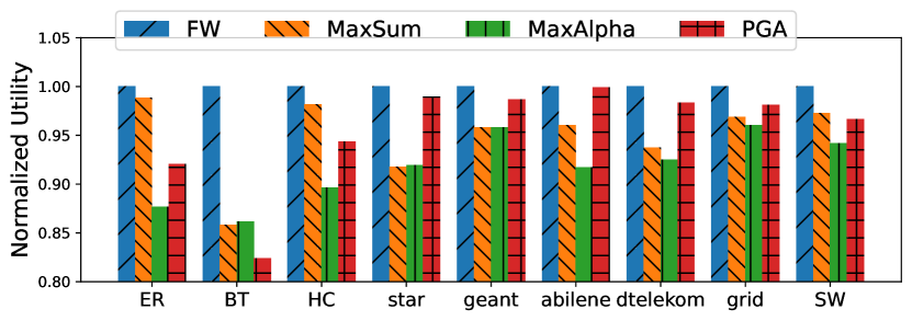
(a) Normalized Aggregate Utility

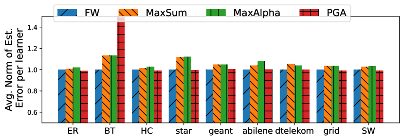
(b) Average Norm of Estimation Error per Learner

Figure 1: Normalized aggregate utility and average norm of estimation error per leaner in different networks. Utilities are normalized by the utility of Algorithm 1 (FW) $U_{\texttt{FW}}$, reported in Table I. We can observe that FW is the best in terms of maximizing the utility and minimizing the estimation error in all networks.

Simulation Parameters. We run FW and PGA for $K=100$ iterations with step size $\delta=0.01$. In each iteration, we estimate the gradient according to Eq. (19) with $N=100$, and $n^{\prime}=\lceil 2\max_{\ell,\boldsymbol{x}}\lambda^{\ell}_{\boldsymbol{x}}T\rceil$, where $\lambda^{\ell}_{\boldsymbol{x}}$ is given by the current solution. We consider a data acquisition time $T=10$. Since our objective function cannot be computed in closed-form, we rely on sampling with $1000$ samples. We also evaluate the model training quality by the average norm of estimation error, where the estimation error is the difference between the true model and the MAP estimator, given by (2). We average over 1000 realizations of the label noise as well as the number of data arrived at the learner $\{\boldsymbol{n}^{\ell}\}_{\ell\in\mathcal{L}}$.

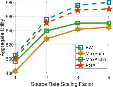
(a) Utility - Source Rates

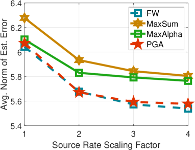
(b) Est. Error - Source Rates

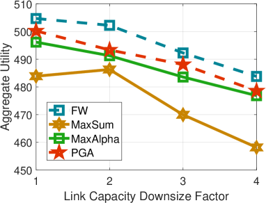
(c) Utility - Link Capacities

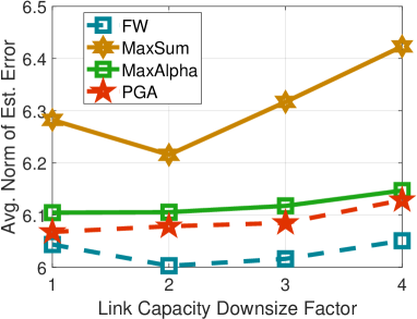
(d) Est. Error - Link Capacities

Figure 2: Algorithm comparison in abilene topology with different parameter settings. The achieved aggregate utility and model estimation quality of different algorithms are evaluated with different source data rates and bottleneck link capacities.

VII-B Results

Performance over Different Topologies. We first compare the proposed algorithm (FW) with baselines in terms of the normalized aggregated utility and model estimation quality over several networks, shown in Figures 1(a) and 1(b), respectively. Utilities in Fig. 1(a) are normalized by the aggregate utility of FW, reported in Tab. I under $U_{\texttt{FW}}$. Learners in these networks have distinct target models to train. In all network topologies, FW outperforms MaxSum and MaxAlpha in both aggregate utility and average norm of estimation error. PGA, which also is based on our experimental design framework, performs well (second best) in most networks, except balanced tree, in which it finds a bad stationary point.

Effect of Source Rates and Link Capacities. Next, we evaluate how algorithm performance is affected by varying source rates as well as link capacitites. We focus on the Abilene network, having 3 sources and 3 learners, where two of the learners have a same target training model. We set the data acquisition time to $T=1$, and labels are generated with Gaussian noise with variance 1. Finally, we again use diagonal prior covariances, and again split between high-variance (selected uniformly between 1 and 3) and low-variance (selected uniformly between 0 and 0.1) features.

Figures 2(a) and 2(b) plot the aggregate utility and average total norm of estimation error across learners, with different data source rates at the sources. The initial source rates are sampled u.a.r. from 2 to 5, and we scale it by different scaling factors. As the source rates increases, the aggregate utility increases and the norm of estimation error decreases for all algorithms. FW is always the best in both figures. Moreover, the proposed experimental design framework can significantly improve the training quality: algorithms based on our proposed framework (FW and PGA) with source rates scaled by $2$ already outperform the other two algorithms (MaxSum and MaxAlpha) with source rates scaled by $4$. We see reverse results of MaxSum and MaxAlpha in these two figures compared with Figure 1, showing that the algorithm which considers fairness (i.e., $\alpha$-fair utilities), may perform better if we have competing learners.

Figures 2(c) and 2(d) show performance in Abilene network with different link capacities of several bottleneck links. The capacities are initially sampled u.a.r. from 50 to 100, and we divide it by different downsize factors. The overall trend is that as the link capacities decrease, algorithms achieve smaller aggregate network utility and get a higher average norm of estimation error. The proposed algorithm is always the best with different bottleneck link capacities in both figures.

VIII Conclusion

We propose experimental design networks, to determine a data transmission strategy that maximizes the quality of trained models in a distributed learning system. The underlying optimization problem can be approximated even though its objective function is non-concave.

Beyond extensions we have already listed, our framework can be used to explore other experimental design objectives (e.g., A-optimality and E-optimality) as well as variants that include data source generation costs. Distributed and adaptive implementations of the rate allocation schemes we proposed are also interesting future directions. Incorporating non-linear learning tasks (e.g., deep neural networks) is also an open avenue of exploration: though Bayesian posteriors are harder to compute in closed-form for this case, techniques such as variational inference [50] can be utilized to approach this problem. Finally, an interesting extension of our model involves a multi-stage setting, in which learners receive data in one stage, update their posteriors, and use these as new priors in the next stage. Studying the dynamics of such a system, as well as how network design impacts these dynamics, is a very interesting open problem.

-A Proof of Lemma 1

Proof.

We extend the proof in Appendix A of [9] for the supmodularity of D-optimal design over a set to the integer lattice: For $\boldsymbol{n}\in\mathbb{N}^{p}$ and $k\in\mathbb{N}$, we have

$$G(\boldsymbol{n} +k\boldsymbol{e}_{i})-G(\boldsymbol{n})=$$

$$= \log\det(\mathbf{I}_{d}+\frac{k}{\sigma^{2}}\boldsymbol{x}_{i}\boldsymbol{x}_{i}^{\top}(\Sigma_{0}^{-1}+\sum_{i=1}^{p}\frac{n_{i}}{\sigma^{2}}\boldsymbol{x}_{i}\boldsymbol{x}_{i}^{\top})^{-1})$$

$$= \log(1+\frac{k}{\sigma^{2}}\boldsymbol{x}_{i}^{\top}A(\boldsymbol{n})^{-1}\boldsymbol{x}_{i}),$$

where $A(\boldsymbol{n})=\Sigma_{0}^{-1}+\sum_{i=1}^{p}\frac{n_{i}}{\sigma^{2}}\boldsymbol{x}_{i}\boldsymbol{x}_{i}^{\top}$, and the last equality follows Eq. (24) in [51]. The monotonicity of $G$ follows because $A(\boldsymbol{n})^{-1}$ is positive semidefinite. Finally, since the matrix inverse is decreasing over the positive semi-definite order, we have $A(\boldsymbol{n})^{-1}\succeq A(\boldsymbol{m})^{-1}$, $\forall\ \boldsymbol{n},\boldsymbol{m}\in\mathbb{N}^{p}\ \text{and}\ \boldsymbol{n}\leq\boldsymbol{m}$, which leads to $G(\boldsymbol{n}+k\boldsymbol{e}_{i})-G(\boldsymbol{n})\geq G(\boldsymbol{m}+k\boldsymbol{e}_{i})-G(\boldsymbol{m})$. ∎

-B Proof of Lemma 2

Proof.

To start with, $\boldsymbol{\lambda}^{K}\in\mathcal{D}$, as a convex combination of points in $\mathcal{D}$. Next, consider the point $\boldsymbol{v}^{*}=(\boldsymbol{\lambda}^{*}\lor\boldsymbol{\lambda})-\boldsymbol{\lambda}=(\boldsymbol{\lambda}^{*}-\boldsymbol{\lambda})\lor\boldsymbol{0}\geq\boldsymbol{0}$, in which $\boldsymbol{\lambda}$ is the solution at current iteration and $\boldsymbol{\lambda}^{*}\in\mathcal{D}$ is the optimal solution. Because $U$ is non-decreasing (Thm. 1), we have

$$U(\boldsymbol{\lambda}+\boldsymbol{v}^{*})=U(\boldsymbol{\lambda}^{*}\lor\boldsymbol{\lambda})\geq U(\boldsymbol{\lambda}^{*}).$$ (33)

A DR-submodular continuous function is concave along any non-negative direction, and any non-positive direction (see e.g., Prop. 4 in [14]), thus $g(\xi):=U(\boldsymbol{\lambda}+\xi\boldsymbol{v}^{*})$, where $g^{\prime}(\xi)=\langle\boldsymbol{v}^{*},\nabla U(\boldsymbol{\lambda}+\xi\boldsymbol{v}^{*})\rangle$, is concave, hence,

$$U(\boldsymbol{\lambda}^{*})-U(\boldsymbol{\lambda})=g(1)-g(0)\leq g^{\prime}(0)\times 1=\langle\boldsymbol{v}^{*},\nabla U(\boldsymbol{\lambda})\rangle.$$ (34)

Then,

$$\langle\boldsymbol{v},\nabla U(\boldsymbol{\lambda})\rangle\overset{\eqref{eq: estimator guarantee short}}{\geq}a\max_{\boldsymbol{v}\in\mathcal{D}}\langle\boldsymbol{v},\nabla U(\boldsymbol{\lambda})\rangle-b\geq a\langle\boldsymbol{\lambda}^{*},\nabla U(\boldsymbol{\lambda})\rangle-b$$

$$\geq a\langle\boldsymbol{v}^{*},\nabla U(\boldsymbol{\lambda})\rangle-b\overset{\eqref{eq: concave}}{\geq}a(U(\boldsymbol{\lambda}+\boldsymbol{v}^{*})-U(\boldsymbol{\lambda}))-b$$

$$\overset{\eqref{eq: optimal}}{\geq}a(U(\boldsymbol{\lambda}^{*})-U(\boldsymbol{\lambda}))-b,$$ (35)

where the second inequality is because the LHS maximizes the inner product and the third inequality is because $\boldsymbol{0}\leq\boldsymbol{v}^{*}\leq\boldsymbol{\lambda}^{*}$ and $\nabla U(\boldsymbol{\lambda})$ is positive (Thm. 1). From the definition of the Hessian, we can show that $||\nabla^{2}U||_{F}$ is bounded by $\sqrt{2}{|\mathcal{X}|}|\mathcal{L}|TG_{\mathrm{MAX}}$ (because 2-norm is smaller than Frobenius norm [52]), thus $L=\sqrt{2}{|\mathcal{X}|}|\mathcal{L}|TG_{\mathrm{MAX}}$ is the Lipschitz continuous constant of $\nabla U$ . Then, we have

$$U(\boldsymbol{\lambda}^{k+1})-U(\boldsymbol{\lambda}^{k})=U(\boldsymbol{\lambda}^{k}+\gamma_{k}\boldsymbol{v}^{k})-U(\boldsymbol{\lambda}^{k})$$

$$\geq\gamma_{k}\langle\boldsymbol{v}^{k},\nabla U(\boldsymbol{\lambda}^{k})\rangle-\frac{L}{2}\gamma_{k}^{2}||\boldsymbol{v}^{k}||_{2}^{2}\text{ (Lipschitz) }$$

$$\overset{\eqref{eq: algorithm update quality}}{\geq}a\gamma_{k}(\max_{\boldsymbol{\lambda}\in\mathcal{D}}U(\boldsymbol{\lambda})-U(\boldsymbol{\lambda}^{k}))-\gamma_{k}b-\frac{L}{2}\gamma_{k}^{2}||\boldsymbol{v}^{k}||_{2}^{2}$$

After rearrangement, we have

$$U(\boldsymbol{\lambda}^{k+1})-\max_{\boldsymbol{\lambda}\in\mathcal{D}}U(\boldsymbol{\lambda})\geq$$

$$(1-a\gamma_{k})[U(\boldsymbol{\lambda}^{k})-\max_{\boldsymbol{\lambda}\in\mathcal{D}}U(\boldsymbol{\lambda})]-\gamma_{k}b-\frac{L}{2}\gamma_{k}^{2}\lambda_{\mathrm{MAX}}^{2},$$

since $||\boldsymbol{v}^{k}||_{2}^{2}\leq\lambda_{\mathrm{MAX}}^{2}$. By telescope,

$$U(\boldsymbol{\lambda}^{K})-\max_{\boldsymbol{\lambda}\in\mathcal{D}}U(\boldsymbol{\lambda})\geq$$

$$[U(\boldsymbol{\lambda}^{0})-\max_{\boldsymbol{\lambda}\in\mathcal{D}}U(\boldsymbol{\lambda})]e^{-a}-b-\frac{L}{2}\sum_{k=0}^{K-1}\gamma_{k}^{2}\lambda_{\mathrm{MAX}}^{2}.$$

Finally, as $U(\boldsymbol{\lambda}^{0})=0$ and $\gamma_{k}=\delta=1/K$, we have

$$U(\boldsymbol{\lambda}^{K})\geq(1-e^{-a})U(\boldsymbol{\lambda}^{*})-\frac{L}{2}\delta\lambda_{\mathrm{MAX}}^{2}-b.$$

∎

-C Proof of Lemma 4

Proof.

We further define

$$\mathrm{TAIL}^{\ell}_{\boldsymbol{x}}=\sum_{n=n^{{}^{\prime}}+1}^{\infty}\Delta^{\ell}_{\boldsymbol{x}}(\boldsymbol{\lambda}^{\ell},n)\cdot T\cdot\mathrm{Pr}[n^{\ell}_{\boldsymbol{x}}=n].$$

We have

$$\mathrm{HEAD}^{\ell}_{\boldsymbol{x}}\geq\Delta^{\ell}_{\boldsymbol{x}}(\boldsymbol{\lambda}^{\ell},n^{\prime})\cdot T\cdot\mathrm{Pr}[n^{\ell}_{\boldsymbol{x}}\leq n^{\prime}]$$

and

$$\mathrm{TAIL}^{\ell}_{\boldsymbol{x}}\leq\Delta^{\ell}_{\boldsymbol{x}}(\boldsymbol{\lambda}^{\ell},n^{\prime})\cdot T\cdot\mathrm{Pr}[n^{\ell}_{\boldsymbol{x}}\geq n^{\prime}+1],$$

since $\Delta^{\ell}_{\boldsymbol{x}}(\boldsymbol{\lambda}^{\ell},t_{1})\geq\Delta^{\ell}_{\boldsymbol{x}}(\boldsymbol{\lambda}^{\ell},t_{2})$ for $t_{1}\leq t_{2}$, resulting from the submodularity of $G$ (Lemma 1). We note that $\frac{\partial U}{\partial\lambda^{\ell}_{\boldsymbol{x}}}=\mathrm{HEAD}^{\ell}_{\boldsymbol{x}}+\mathrm{TAIL}^{\ell}_{\boldsymbol{x}}$. Then we have,

$$\frac{\mathrm{HEAD}^{\ell}_{\boldsymbol{x}}}{\mathrm{HEAD}^{\ell}_{\boldsymbol{x}}+\mathrm{TAIL}^{\ell}_{\boldsymbol{x}}}=\frac{1}{1+\frac{\mathrm{TAIL}^{\ell}_{\boldsymbol{x}}}{\mathrm{HEAD}^{\ell}_{\boldsymbol{x}}}}\geq$$

$$\frac{1}{1+\frac{\Delta^{\ell}_{\boldsymbol{x}}(\boldsymbol{\lambda}^{\ell},n^{\prime})\cdot T\cdot\mathrm{Pr}[n^{\ell}_{\boldsymbol{x}}\geq n^{\prime}+1]}{\Delta^{\ell}_{\boldsymbol{x}}(\boldsymbol{\lambda}^{\ell},n^{\prime})\cdot T\cdot(1-\mathrm{Pr}[n^{\ell}_{\boldsymbol{x}}\geq n^{\prime}+1]})}=1-\mathrm{Pr}[n^{\ell}_{\boldsymbol{x}}\geq n^{\prime}+1],$$

thus,

$$\mathrm{HEAD}^{\ell}_{\boldsymbol{x}} \geq(1-\mathrm{Pr}[n^{\ell}_{\boldsymbol{x}}\geq n^{\prime}+1])\frac{\partial U}{\partial\lambda^{\ell}_{\boldsymbol{x}}}$$

$$\geq(1-e^{-\frac{(n^{\prime}-\lambda^{\ell}_{\boldsymbol{x}}T+1)^{2}}{2\lambda^{\ell}_{\boldsymbol{x}}T}h(\frac{n^{\prime}-\lambda^{\ell}_{\boldsymbol{x}}T+1}{\lambda^{\ell}_{\boldsymbol{x}}T})})\frac{\partial U}{\partial\lambda^{\ell}_{\boldsymbol{x}}},$$

where $h(u)=2\frac{(1+u)\ln{(1+u)}-u}{u^{2}}$ (Lemma 3). ∎

-D Proof of Lemma 5

Proof.

Our final estimator of the partial derivative is given by

$$\widehat{\frac{\partial U}{\partial\lambda^{\ell}_{\boldsymbol{x}}}}\equiv T\sum_{n=0}^{n^{\prime}}\widehat{\Delta^{\ell}_{\boldsymbol{x}}(\boldsymbol{\lambda}^{\ell},n)}\mathrm{Pr}[n^{\ell}_{\boldsymbol{x}}=n],$$

where

$$\widehat{\Delta^{\ell}_{\boldsymbol{x}}(\boldsymbol{\lambda}^{\ell},n)}=\frac{1}{N}\sum_{j=1}^{N}(G^{\ell}(\boldsymbol{n}^{\ell,j}|_{n_{\boldsymbol{x}}^{\ell,j}=n+1})-G^{\ell}(\boldsymbol{n}^{\ell,j}|_{n_{\boldsymbol{x}}^{\ell,j}=n})).$$

We define

$$\textstyle X^{j}(n)=\frac{G^{\ell}(\boldsymbol{n}^{\ell,j}|_{n^{\ell,j}_{\boldsymbol{x}}=n+1})-G^{\ell}(\boldsymbol{n}^{\ell,j}|_{n_{\boldsymbol{x}}^{\ell,j}=n})-\Delta^{\ell}_{\boldsymbol{x}}(\boldsymbol{\lambda}^{\ell},t)}{G_{\mathrm{MAX}}},$$

where

$$G_{\mathrm{MAX}}=\max_{\ell\in\mathcal{L},\boldsymbol{x}\in\mathcal{X}}(G^{\ell}(\boldsymbol{e}_{\boldsymbol{x}})-G^{\ell}(\boldsymbol{0})).$$

We have $|X^{j}(n)|\leq 1$, because

$$G_{\mathrm{MAX}} \geq G^{\ell}(\boldsymbol{e}_{\boldsymbol{x}})-G^{\ell}(\boldsymbol{0})$$

$$\geq G^{\ell}(\boldsymbol{n}^{\ell}|n_{\boldsymbol{x}}=n+1)-G^{\ell}(\boldsymbol{n}^{\ell}|n_{\boldsymbol{x}}=n),$$

for any $\ell\in\mathcal{L},\boldsymbol{x}\in\mathcal{X}$, $n\geq 0$. By Chernoff bounds described by Theorem A.1.16 in [45], we have

$$\mathrm{Pr}\left[\left|\sum_{j=1}^{N}\sum_{n=0}^{n=n^{\prime}}X^{j}(n)\right|>c\right]\leq 2e^{-c^{2}/2N(n^{{}^{\prime}}+1)}.$$

Suppose we let $c=\delta\cdot N/T$, where $\delta$ is the step size, then we have

$$|\widehat{\frac{\partial U}{\partial\lambda^{\ell}_{\boldsymbol{x}}}}-\mathrm{HEAD}^{\ell}_{\boldsymbol{x}}|$$

$$\leq \left|\sum_{n=0}^{n^{\prime}}\sum_{j=1}^{N}\textstyle\frac{(G^{\ell}(\boldsymbol{n}^{\ell,j}|_{n^{\ell,j}_{\boldsymbol{x}}=n+1})-G^{\ell}(\boldsymbol{n}^{\ell,j}|_{n_{\boldsymbol{x}}^{\ell,j}=n})-\Delta^{\ell}_{\boldsymbol{x}}(\boldsymbol{\lambda}^{\ell},n))}{N}T\right|$$

$$= \textstyle\left|\sum_{t=0}^{n^{\prime}}\sum_{j=1}^{N}X^{j}(n)\right|\cdot\frac{T}{N}\cdot G_{\mathrm{MAX}}\leq\delta\cdot G_{\mathrm{MAX}},$$

with probability greater than $1-2\cdot e^{-\delta^{2}N/2T^{2}(n^{\prime}+1)}$. By Lemma 4, we have $\mathrm{HEAD}^{\ell}_{\boldsymbol{x}}\geq(1-\mathrm{P}[n^{\ell}_{\boldsymbol{x}}\geq n^{\prime}+1])\cdot\frac{\partial U}{\partial\lambda^{\ell}_{\boldsymbol{x}}}$. Thus, we have

$$\textstyle-\delta\cdot G_{\mathrm{MAX}}\leq\frac{\partial U}{\partial\lambda^{\ell}_{\boldsymbol{x}}}-\widehat{\frac{\partial U}{\partial\lambda^{\ell}_{\boldsymbol{x}}}}\leq\delta\cdot G_{\mathrm{MAX}}+\mathrm{Pr}[n^{\ell}_{\boldsymbol{x}}\geq n^{\prime}+1]\cdot\frac{\partial U}{\partial\lambda^{\ell}_{\boldsymbol{x}}}.$$ (36)

We now use the superscript $k$ to represent the parameters for the $k$th iteration: we find $\boldsymbol{v}^{k}\in\mathcal{D}$ that maximizes $\langle\boldsymbol{v}^{k},\widehat{\nabla U(\boldsymbol{\lambda}^{k})}\rangle$. Let $\boldsymbol{u}^{k}\in\mathcal{D}$ be the vector that maximizes $\langle\boldsymbol{u}^{k},\nabla U(\boldsymbol{\lambda}^{k})\rangle$ instead and define $\mathrm{P_{MAX}}=\max_{k=1,\dots,K}\mathrm{P}^{k}_{\mathrm{MAX}}$ where $\mathrm{P}^{k}_{\mathrm{MAX}}=\max_{l\in\mathcal{L},\boldsymbol{x}\in\mathcal{X}}\mathrm{P}[n^{\ell,k}_{\boldsymbol{x}}\geq t^{\prime}+1]$ and $\lambda_{\mathrm{MAX}}\equiv\max_{\boldsymbol{\lambda}\in\mathcal{D}}\sum_{\ell\in\mathcal{L}}||\boldsymbol{\lambda}^{\ell}||_{1}$. We have

$$\langle\boldsymbol{v}^{k},\nabla U(\boldsymbol{\lambda}^{k})\rangle\geq\langle\boldsymbol{v}^{k},\widehat{\nabla U(\boldsymbol{\lambda}^{k})}\rangle-\lambda_{\text{MAX}}\delta\cdot G_{\mathrm{MAX}}$$

$$\geq \langle\boldsymbol{u}^{k},\widehat{\nabla U(\boldsymbol{\lambda}^{k})}\rangle-\lambda_{\text{MAX}}\delta\cdot G_{\mathrm{MAX}}$$

$$\geq (1-\mathrm{P_{MAX}})\cdot\langle\boldsymbol{u}^{k},\nabla U(\boldsymbol{\lambda}^{k})\rangle-2\lambda_{\text{MAX}}\delta\cdot G_{\mathrm{MAX}},$$

where the first and last inequalities are due to (36) and the second inequality is because $\boldsymbol{v}^{k}$ maximizes $\langle\boldsymbol{v}^{k},\widehat{\nabla U(\boldsymbol{\lambda}^{k})}\rangle$. The above inequality requires the satisfaction of (36) for every partial derivative. By union bound, the above inequality satisfies with probability greater than $1-2|\mathcal{X}||\mathcal{L}|\cdot e^{-\delta^{2}N/2T^{2}(n^{\prime}+1)}$. ∎

References

• [1] N. Abbas, Y. Zhang, A. Taherkordi, and T. Skeie, “Mobile edge computing: A survey,” IEEE Internet of Things Journal, vol. 5, no. 1, pp. 450–465, 2017.
• [2] B. Yang, X. Cao, X. Li, Q. Zhang, and L. Qian, “Mobile-edge-computing-based hierarchical machine learning tasks distribution for iiot,” IEEE Internet of Things Journal, vol. 7, no. 3, pp. 2169–2180, 2019.
• [3] V. Albino, U. Berardi, and R. M. Dangelico, “Smart cities: Definitions, dimensions, performance, and initiatives,” Journal of urban technology, vol. 22, no. 1, pp. 3–21, 2015.
• [4] M. Mohammadi and A. Al-Fuqaha, “Enabling cognitive smart cities using big data and machine learning: Approaches and challenges,” IEEE Communications Magazine, vol. 56, no. 2, pp. 94–101, 2018.
• [5] S. Boyd, S. P. Boyd, and L. Vandenberghe, Convex optimization.   Cambridge university press, 2004.
• [6] Y. Deshpande and A. Montanari, “Linear bandits in high dimension and recommendation systems,” in 2012 50th Annual Allerton Conference on Communication, Control, and Computing (Allerton).   IEEE, 2012, pp. 1750–1754.
• [7] B. Settles, Active learning literature survey.   Computer Sciences Technical Report 1648, University of Wisconsin-Madison, 2009.
• [8] N. Polyzotis, S. Roy, S. E. Whang, and M. Zinkevich, “Data lifecycle challenges in production machine learning: a survey,” ACM SIGMOD Record, vol. 47, no. 2, pp. 17–28, 2018.
• [9] T. Horel, S. Ioannidis, and S. Muthukrishnan, “Budget feasible mechanisms for experimental design,” in Latin American Symposium on Theoretical Informatics.   Springer, 2014, pp. 719–730.
• [10] Y. Guo, J. Dy, D. Erdogmus, J. Kalpathy-Cramer, S. Ostmo, J. P. Campbell, M. F. Chiang, and S. Ioannidis, “Accelerated experimental design for pairwise comparisons,” in Proceedings of the 2019 SIAM International Conference on Data Mining.   SIAM, 2019, pp. 432–440.
• [11] N. Gast, S. Ioannidis, P. Loiseau, and B. Roussillon, “Linear regression from strategic data sources,” ACM Transactions on Economics and Computation (TEAC), vol. 8, no. 2, pp. 1–24, 2020.
• [12] Y. Guo, P. Tian, J. Kalpathy-Cramer, S. Ostmo, J. P. Campbell, M. F. Chiang, D. Erdogmus, J. G. Dy, and S. Ioannidis, “Experimental design under the bradley-terry model.” in IJCAI, 2018, pp. 2198–2204.
• [13] P. Flaherty, A. Arkin, and M. I. Jordan, “Robust design of biological experiments,” in Advances in neural information processing systems, 2006, pp. 363–370.
• [14] A. A. Bian, B. Mirzasoleiman, J. Buhmann, and A. Krause, “Guaranteed non-convex optimization: Submodular maximization over continuous domains,” in Artificial Intelligence and Statistics.   PMLR, 2017, pp. 111–120.
• [15] L. Tong, Y. Li, and W. Gao, “A hierarchical edge cloud architecture for mobile computing,” in IEEE INFOCOM 2016-IEEE International Conference on Computer Communications, 2016, pp. 1–9.
• [16] K. Poularakis, J. Llorca, A. M. Tulino, I. Taylor, and L. Tassiulas, “Joint service placement and request routing in multi-cell mobile edge computing networks,” in IEEE INFOCOM 2019-IEEE Conference on Computer Communications, 2019, pp. 10–18.
• [17] K. Kamran, E. Yeh, and Q. Ma, “Deco: Joint computation, caching and forwarding in data-centric computing networks,” in Proceedings of the Twentieth ACM International Symposium on Mobile Ad Hoc Networking and Computing, 2019, pp. 111–120.
• [18] A. Lalitha, O. C. Kilinc, T. Javidi, and F. Koushanfar, “Peer-to-peer federated learning on graphs,” arXiv preprint arXiv:1901.11173, 2019.
• [19] G. Neglia, G. Calbi, D. Towsley, and G. Vardoyan, “The role of network topology for distributed machine learning,” in IEEE INFOCOM 2019-IEEE Conference on Computer Communications, 2019, pp. 2350–2358.
• [20] S. Wang, T. Tuor, T. Salonidis, K. K. Leung, C. Makaya, T. He, and K. Chan, “When edge meets learning: Adaptive control for resource-constrained distributed machine learning,” in IEEE INFOCOM 2018-IEEE Conference on Computer Communications, 2018, pp. 63–71.
• [21] K. Zhang, Z. Yang, H. Liu, T. Zhang, and T. Basar, “Fully decentralized multi-agent reinforcement learning with networked agents,” in International Conference on Machine Learning.   PMLR, 2018, pp. 5872–5881.
• [22] S. Wang, Y. Ruan, Y. Tu, S. Wagle, C. G. Brinton, and C. Joe-Wong, “Network-aware optimization of distributed learning for fog computing,” IEEE/ACM Transactions on Networking, 2021.
• [23] F. Pukelsheim, Optimal design of experiments.   Society for Industrial and Applied Mathematics, 2006.
• [24] X. Huan and Y. M. Marzouk, “Simulation-based optimal bayesian experimental design for nonlinear systems,” Journal of Computational Physics, vol. 232, no. 1, pp. 288–317, 2013.
• [25] G. L. Nemhauser, L. A. Wolsey, and M. L. Fisher, “An analysis of approximations for maximizing submodular set functions—i,” Mathematical programming, vol. 14, no. 1, pp. 265–294, 1978.
• [26] G. Calinescu, C. Chekuri, M. Pal, and J. Vondrák, “Maximizing a monotone submodular function subject to a matroid constraint,” SIAM Journal on Computing, vol. 40, no. 6, pp. 1740–1766, 2011.
• [27] T. Soma and Y. Yoshida, “A generalization of submodular cover via the diminishing return property on the integer lattice,” Advances in neural information processing systems, vol. 28, pp. 847–855, 2015.
• [28] H. Hassani, M. Soltanolkotabi, and A. Karbasi, “Gradient methods for submodular maximization,” in Proceedings of the 31st International Conference on Neural Information Processing Systems, 2017, pp. 5843–5853.
• [29] A. A. Ageev and M. I. Sviridenko, “Pipage rounding: A new method of constructing algorithms with proven performance guarantee,” Journal of Combinatorial Optimization, vol. 8, no. 3, pp. 307–328, 2004.
• [30] C. Chekuri, J. Vondrák, and R. Zenklusen, “Dependent randomized rounding via exchange properties of combinatorial structures,” in 2010 IEEE 51st Annual Symposium on Foundations of Computer Science.   IEEE, 2010, pp. 575–584.
• [31] T. Soma and Y. Yoshida, “Maximizing monotone submodular functions over the integer lattice,” Mathematical Programming, vol. 172, no. 1, pp. 539–563, 2018.
• [32] S. Ioannidis and E. Yeh, “Adaptive caching networks with optimality guarantees,” IEEE/ACM Transactions on Networking, vol. 26, no. 2, pp. 737–750, 2018.
• [33] K. Poularakis and L. Tassiulas, “On the complexity of optimal content placement in hierarchical caching networks,” IEEE Transactions on Communications, vol. 64, no. 5, pp. 2092–2103, 2016.
• [34] S. Ioannidis and E. Yeh, “Jointly optimal routing and caching for arbitrary network topologies,” IEEE Journal on Selected Areas in Communications, vol. 36, no. 6, pp. 1258–1275, 2018.
• [35] K. Kamran, A. Moharrer, S. Ioannidis, and E. Yeh, “Rate allocation and content placement in cache networks,” in IEEE INFOCOM, 2021.
• [36] T. Wu, P. Yang, H. Dai, W. Xu, and M. Xu, “Charging oriented sensor placement and flexible scheduling in rechargeable wsns,” in IEEE INFOCOM 2019-IEEE Conference on Computer Communications, 2019, pp. 73–81.
• [37] G. Sallam and B. Ji, “Joint placement and allocation of virtual network functions with budget and capacity constraints,” in IEEE INFOCOM 2019-IEEE Conference on Computer Communications, 2019, pp. 523–531.
• [38] Z. Zheng and N. B. Shroff, “Submodular utility maximization for deadline constrained data collection in sensor networks,” IEEE Transactions on Automatic Control, vol. 59, no. 9, pp. 2400–2412, 2014.
• [39] D. Yang, G. Xue, X. Fang, and J. Tang, “Crowdsourcing to smartphones: Incentive mechanism design for mobile phone sensing,” in Proceedings of the 18th annual international conference on Mobile computing and networking, 2012, pp. 173–184.
• [40] A. Krause and C. Guestrin, “Beyond convexity: Submodularity in machine learning,” ICML Tutorials, 2008.
• [41] G. James, D. Witten, T. Hastie, and R. Tibshirani, An introduction to statistical learning.   Springer, 2013, vol. 112.
• [42] R. G. Gallager, Stochastic processes: theory for applications.   Cambridge University Press, 2013.
• [43] F. P. Kelly, Reversibility and stochastic networks.   Cambridge University Press, 2011.
• [44] C. L. Canonne, “A short note on poisson tail bounds,” http://www.cs.columbia.edu/~ccanonne/files/misc/2017-poissonconcentration.pdf.
• [45] N. Alon and J. H. Spencer, The probabilistic method.   John Wiley & Sons, 2004.
• [46] J. Friedman, T. Hastie, R. Tibshirani et al., The elements of statistical learning.   Springer series in statistics New York, 2001, vol. 1, no. 10.
• [47] J. Kleinberg, “The small-world phenomenon: An algorithmic perspective,” Cornell University, Tech. Rep., 1999.
• [48] D. Rossi and G. Rossini, “Caching performance of content centric networks under multi-path routing (and more),” Relatório técnico, Telecom ParisTech, pp. 1–6, 2011.
• [49] R. Srikant, The Mathematics of Internet Congestion Control.   Birkhäuser Boston, MA: Springer Science & Business Media, 2012.
• [50] T. S. Jaakkola and M. I. Jordan, “A variational approach to bayesian logistic regression models and their extensions,” in Sixth International Workshop on Artificial Intelligence and Statistics.   PMLR, 1997, pp. 283–294.
• [51] K. B. Petersen and M. S. Pedersen, “The matrix cookbook (version: November 15, 2012),” 2012.
• [52] R. A. Horn and C. R. Johnson, Matrix analysis.   Cambridge university press, 2012.