Lepton Number vs Coulomb Super-Criticality

Abstract

The non-perturbative effects of QED-vacuum reconstruction under influence of a supercritical EM-source ($Z>Z_{cr,1}$) are considered in view of lepton number conservation. The question is here that if the vacuum shells formation and spontaneous positron emission, associated with discrete levels diving into the lower continuum, exist in reality, then it by no means should be a signal of new physics. The reason is that the emitted positrons carry away the lepton number equal to $(-1)\times$their total number, and so the corresponding amount of positive lepton number should be shared by VP-density, concentrated in vacuum shells. In this case instead of integer lepton number of real particles there should appear the lepton number VP-density. Otherwise either the lepton number conservation in such processes must be broken, or the spontaneous positron emission prohibited. The conditions, under which the emission of vacuum positrons can be unambiguously detected on the nuclear conversion pairs background, are also discussed.

I Introduction

Nowadays the behavior of QED-vacuum under influence of a supercritical EM-source is subject to an active research Rafelski et al. (2017); Kuleshov et al. (2015a); *Kuleshov2015b; *Godunov2017; Davydov et al. (2017); *Sveshnikov2017; *Voronina2017; Popov et al. (2018); *Novak2018; *Maltsev2018; Roenko and Sveshnikov (2018); Maltsev et al. (2019); *Maltsev2020. Of the main interest is that in such external fields there should take place a deep vacuum state reconstruction, caused by discrete levels diving into the lower continuum and accompanied by such nontrivial effects as spontaneous positron emission combined with vacuum shells formation (see e.g., Refs. Greiner et al. (1985); Plunien et al. (1986); Greiner and Reinhardt (2009); Ruffini et al. (2010); Rafelski et al. (2017) and citations therein). In 3+1 QED such effects are expected for extended Coulomb sources of nucleus size with charges $Z>Z_{cr,1}\simeq 170$, which are large enough for direct observation and probably could be created in low energy heavy ions collisions at new heavy ion facilities like FAIR (Darmstadt), NICA (Dubna), HIAF (Lanzhou).

The aim of the present paper is to figure out the main consequences of such non-perturbative VP-effects with emphasis on lepton number conservation. This question appears naturally since the most important result of discrete levels diving into the lower continuum beyond the threshold of super-criticality is the vacuum shells formation accompanied by spontaneous positron emission. At the same time, the emitted positrons carry away the lepton number equal to $(-1)\times$their total number, and so the corresponding amount of positive lepton number should be shared by VP-density, concentrated in vacuum shells. In this case instead of integer lepton number of real particles ($e$-, $\mu$-, $\tau$-leptons, corresponding neutrinos and their antiparticles) there appears the lepton number VP-density. Otherwise either the lepton number conservation in such processes must be broken, or the positron emission prohibited. Therefore the reliable observation of vacuum positrons could shed light on the nature of lepton number, which as well as the baryon one, is so far just a number, but not a conserved charge, associated with certain type of symmetry. So the reasonable conditions, under which the vacuum positron emission can be unambiguously detected on the nuclear conversion pairs background, should play an exceptional role in slow ions collisions, aimed at the search of such events.

In the present paper this problem is explored within the Dirac-Coulomb problem (DC) with external static or adiabatically slowly varying spherically-symmetric Coulomb potential, created by uniformly charged sphere

$$V(r)=-Z\alpha\,\left({1\over R(Z)}\,\theta(R(Z)-r)+{1\over r}\,\theta(r-R(Z))\right)\ ,$$ (1)

or charged ball with

$$V(r)=-Z\alpha\,\left({3\,R^{2}(Z)-r^{2}\over 2\,R^{3}(Z)}\,\theta(R(Z)-r)\ +\right.\\ \left.+\ {1\over r}\,\theta(r-R(Z))\right)\ .$$ (2)

Here and henceforth the relation between the radius of the Coulomb source and its charge is given by

$$R(Z)\simeq 1.2\,(2.5\,|Z|)^{1/3}\ \hbox{fm}\ ,$$ (3)

which roughly imitates the size of super-heavy nucleus with charge $Z$. In what follows $R(Z)$ will be quite frequently denoted simply as $R$.

The non-stationary approach, based on the time-dependent picture created by two heavy ions slowly moving along the classical Rutherford trajectories Reinhardt et al. (1981); *Mueller1988; Ackad and Horbatsch (2008); Popov et al. (2018); *Novak2018; *Maltsev2018; Maltsev et al. (2019); *Maltsev2020, looks more attractive, since it imitates the realistic scenario of attaining the super-critical region in heavy ions collision. At the same time, the VP-effects at short internuclear distances achieved in the monopole approximation are in rather good agreement with exact two-center ones Reinhardt et al. (1981); *Mueller1988; Tupitsyn et al. (2010); Maltsev et al. (2019); *Maltsev2020 and lie always in between those for sphere and ball upon adjusting properly the coefficient in relation (3), because they are very sensitive to the latter. The main advantage of time-dependent approach is $ab\ initio$ description of pairs production caused by Coulomb excitations of nuclei, while in adiabatic picture the latter should be considered as an additional component. However, it will be argued below that the actual threshold for vacuum positrons detection on the conversion pairs background turns out to be not less than $Z^{\ast}\simeq 210$, which lies beyond the existing nowadays opportunities in heavy ion collisions.

As in other works on this topic  Wichmann and Kroll (1956); Gyulassy (1975); Brown et al. (1975a); *McLerran1975b; *McLerran1975c; Greiner et al. (1985); Plunien et al. (1986); Greiner and Reinhardt (2009); Ruffini et al. (2010); Rafelski et al. (2017), radiative corrections from virtual photons are neglected. Henceforth, if it is not stipulated separately, relativistic units $\hbar=m_{e}=c=1$ and the standard representation of Dirac matrices are used. Concrete calculations, illustrating the general picture, are performed for $\alpha=1/137.036$ by means of Computer Algebra Systems (such as Maple 21) to facilitate the analytic calculations and GNU Octave code for boosting the numerical work.

II Vacuum shells formation

The most efficient non-perturbative evaluation of the VP-charge density $\varrho_{VP}(\vec{r})$ is based on the Wichmann and Kroll (WK) approach  Wichmann and Kroll (1956); Gyulassy (1975); Mohr et al. (1998). The starting point of the latter is the vacuum value

$$\varrho_{VP}(\vec{r})=-\frac{|e|}{2}\left(\sum\limits_{\epsilon_{n}<\epsilon_{F}}\psi_{n}(\vec{r})^{\dagger}\psi_{n}(\vec{r})\ -\right.\\ \left.-\ \sum\limits_{\epsilon_{n}\geqslant\epsilon_{F}}\psi_{n}(\vec{r})^{\dagger}\psi_{n}(\vec{r})\right)\ .$$ (4)

In (4) $\epsilon_{F}=-1$ is the Fermi level, which in such problems with strong Coulomb fields is chosen at the lower threshold, while $\epsilon_{n}$ and $\psi_{n}(\vec{r})$ are the eigenvalues and properly normalized set of eigenfunctions of corresponding DC. The expression (4) for the VP-charge density is a direct consequence of the well-known Schwinger prescription for the fermionic current in terms of the fermion fields commutators

$$j_{\mu}(\vec{r},t)=-{|e|\over 2}\,\left[\bar{\psi}(\vec{r},t)\,,\gamma_{\mu}\psi(\vec{r},t)\right]\ .$$ (5)

The essence of the WK techniques is the representation of the density (4) in terms of contour integrals on the first sheet of the Riemann energy plane containing the trace of the Green function of corresponding DC. In our case the Green function is defined via equation

$$\left[-i\vec{\alpha}\,\vec{\nabla}_{r}+\beta+V(r)-\epsilon\right]G(\vec{r},\vec{r}\,^{\prime};\epsilon)\\ =\delta(\vec{r}-\vec{r}\,^{\prime})\ .$$ (6)

The formal solution of (6) reads

$$G(\vec{r},\vec{r}\ ^{\prime};\epsilon)=\sum\limits_{n}\frac{\psi_{n}(\vec{r})\psi_{n}(\vec{r}\ ^{\prime})^{\dagger}}{\epsilon_{n}-\epsilon}\ .$$ (7)

Following Ref. Wichmann and Kroll (1956), the density (4) is expressed via the integrals along the contours $P(R_{0})$ and $E(R_{0})$ on the first sheet of energy surface (Fig.1).

$$\varrho_{VP}(\vec{r})=\\ =-\frac{|e|}{2}\lim_{R_{0}\rightarrow\infty}\left(\frac{1}{2\pi i}\int\limits_{P(R_{0})}\!d\epsilon\,\mathrm{Tr}G(\vec{r},\vec{r^{\prime}};\epsilon)|_{\vec{r^{\prime}}\rightarrow\vec{r}}\ +\right.\\ \left.+\ \frac{1}{2\pi i}\int\limits_{E(R_{0})}\!d\epsilon\,\mathrm{Tr}G(\vec{r},\vec{r^{\prime}};\epsilon)|_{\vec{r^{\prime}}\rightarrow\vec{r}}\right)\ .$$ (8)

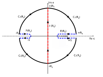
Figure 1: (Color online) WK-contours in the complex energy plane, used for representation of the VP-charge density (4) via contour integrals. The direction of contour integration is chosen in correspondence with (7).

Note that the Green function in this relation must be properly regularized to insure that the limit $\vec{r^{\prime}}\to\vec{r}$ exists and that the integrals over $d\epsilon$ converge. This regularization is discussed below. On this stage, though, all expressions are to be understood to involve only regulated Green functions. One of the main consequences of the last convention is the uniform asymptotics of the integrands in (8) on the large circle $|\epsilon|\to\infty$ at least as $O(1/\epsilon)$, which allows for deforming the contours $P(R_{0})$ and $E(R_{0})$ to the imaginary axis segment $I(R_{0})$ and taking the limit $R_{0}\to\infty$, what gives

$$\varrho_{VP}(\vec{r})=\\ =|e|\left[\sum\limits_{-1\leqslant\epsilon_{n}<0}|\psi_{n}(\vec{r})|^{2}+{1\over 2\pi}\,\int\limits_{-\infty}^{\infty}\!dy\,\mathrm{Tr}G(\vec{r},\vec{r^{\prime}};iy)|_{\vec{r^{\prime}}\rightarrow\vec{r}}\right]\ ,$$ (9)

where $\{\psi_{n}(\vec{r})\}$ are the normalized eigenfunctions of negative discrete levels with $-1\leqslant\epsilon_{n}<0$ and here and henceforth $\psi_{n}(\vec{r})^{\dagger}\psi_{n}(\vec{r})=|\psi_{n}(\vec{r})|^{2}$.

Proceeding further, the Green function (7) is represented as a partial series over $k=\pm(j+1/2)$  Wichmann and Kroll (1956); Gyulassy (1975)

$$\mathrm{Tr}G(\vec{r},\vec{r^{\prime}};\epsilon)|_{\vec{r^{\prime}}\rightarrow\vec{r}}=\sum\limits_{k}{|k|\over 2\pi}\,\mathrm{Tr}G_{k}(r,r^{\prime};\epsilon)|_{r^{\prime}\rightarrow r}\ ,$$ (10)

where the radial Green function $G_{k}(r,r^{\prime};\epsilon)$ is defined via

$$\hbox{$\cal H$}_{k}(r)\,G_{k}(r,r^{\prime};\epsilon)={\delta(r-r^{\prime})\over rr^{\prime}},$$ (11)

while the radial Dirac Hamiltonian takes the form

$$\hbox{$\cal H$}_{k}(r)=\begin{pmatrix}V(r)+1-\epsilon&-{1\over r}\,{d\over dr}\,r-{k\over r}\\ {1\over r}\,{d\over dr}\,r-{k\over r}&V(r)-1-\epsilon\end{pmatrix}\ .$$ (12)

For the partial terms of $\varrho_{VP}(r)$ one obtains

$$\varrho_{VP,k}(r)={|e||k|\over 2\pi}\left[\sum\limits_{-1\leqslant\epsilon_{n,k}<0}|\psi_{n,k}(r)|^{2}+\right.\\ \left.+{1\over 2\pi}\,\int\limits_{-\infty}^{\infty}\!dy\,\mathrm{Tr}G_{k}(r,r^{\prime};iy)|_{r^{\prime}\rightarrow r}\right]\ ,$$ (13)

where $\psi_{n,k}(r)$ are the normalized radial wave functions with eigenvalues $k$ and $\epsilon_{n,k}$ of the corresponding DC. From (13) by means of symmetry relations Gyulassy (1975) for the sum $\varrho_{VP,|k|}(r)$ of two partial VP-densities with opposite signs of $k$ one finds

$$\varrho_{VP,|k|}(r)={|e||k|\over 2\pi}\,\Big{\{}\sum\limits_{k=\pm|k|}\sum\limits_{-1\leqslant\epsilon_{n,k}<0}|\psi_{n,k}(r)|^{2}+\\ +{2\over\pi}\,\int\limits_{0}^{\infty}\!dy\,\mathrm{Re}\left[\mathrm{Tr}G_{k}(r,r^{\prime};iy)\right]|_{r^{\prime}\rightarrow r}\Big{\}}\ ,$$ (14)

which is by construction real and odd in $Z$ (in accordance with the Furry theorem).

The general result, obtained in Ref. Gyulassy (1975) within the expansion of $\varrho_{VP}(\vec{r})$ in powers of $Z\alpha$ (but with fixed radius $R=R(Z)$ !), which is valid for 1+1 and 2+1 D always, and for a spherically-symmetric external potential in the three-dimensional case, is that all the divergencies of $\varrho_{VP}(\vec{r})$ originate from the fermionic loop with two external photon lines, whereas the next-to-leading orders of expansion in $Z\alpha$ are already free from divergencies (see also Ref. Mohr et al. (1998) and refs. therein). In the non-perturbative approach this statement has been verified for 1+1 D in Refs. Davydov et al. (2017); *Sveshnikov2017; *Voronina2017 and for 2+1 D in Refs. Davydov et al. (2018a); *Davydov2018b; Sveshnikov et al. (2019a); *Sveshnikov2019b by means of the phase integral techniques. The latter can be also extended for the present 3+1 D case. From these results there follows first that for any partial Green function $G_{k}$ the deformation of the WK-contours $P(R_{0})$ and $E(R_{0})$ to the imaginary axis can be performed without any ambiguities. Second, the decreasing asymptotics of $\mathrm{Re}\,\left[\hbox{Tr}G_{k}(r,r;iy)\right]$ for $|y|\to\infty$ turns out to be much faster, namely $O(1/|y|^{3})$, than the previously announced one for the regulated Green function $G\left(\vec{r},\vec{r}^{\prime};\epsilon\right)$, which enters the initial WK-contour representation (8). The main reason for such difference is that the properties of $G_{k}$ are much better than for the whole partial series. This circumstance has been discussed earlier in Ref.Gyulassy (1975).

So the renormalization procedure for the VP-density (4) is actually the same for all the three spatial dimensions and reduces to the diagram with two external lines. Thus, in order to find the renormalized $\varrho^{ren}_{VP}(r)$, the linear in external field terms in the expression (9) should be extracted and replaced by the renormalized first-order perturbative density $\varrho^{(1)}_{VP}(r)$, evaluated with the same $R(Z)$. For these purposes let us introduce first the component $\varrho^{(3+)}_{VP,|k|}(r)$ of partial VP-density, which is defined in the next way

$$\varrho_{VP,|k|}^{(3+)}(r)=\frac{|e||k|}{2\pi}\,\Big{\{}\sum\limits_{k=\pm|k|}\sum\limits_{-1\leqslant\epsilon_{n,k}<0}|\psi_{n,k}(r)|^{2}\ +\\ +\ \frac{2}{\pi}\int\limits_{0}^{\infty}dy\,\mathrm{Re}\left[\hbox{Tr}G_{k}(r,r;iy)-\hbox{Tr}G^{(1)}_{k}(r;iy)\right]\Big{\}}\ ,$$ (15)

where $G^{(1)}_{k}(r;iy)$ is the linear in $Z\alpha$ component of the partial Green function $G_{k}(r,r;iy)$ and so coincides with the first term of the Born series

$$G^{(1)}_{k}=G^{(0)}_{k}(-V)G^{(0)}_{k}\ ,$$ (16)

where $G_{k}^{(0)}$ is the free radial Green function with the same $k$ and $\epsilon$. By construction $\varrho^{(3+)}_{VP,|k|}(r)$ contains only odd powers of $Z\alpha$ starting from $n=3$ and so is free of divergencies, but at the same time it is responsible for all the nonlinear effects, which are caused by discrete levels diving into the lower continuum.

As a result, the renormalized VP-charge density $\varrho^{ren}_{VP}(r)$ is defined by the following expression

$$\varrho^{ren}_{VP}(r)=\varrho_{VP}^{(1)}(r)+\sum\limits_{k=1}^{\infty}\varrho_{VP,|k|}^{(3+)}(r)\ ,$$ (17)

where $\varrho_{VP}^{(1)}(r)$ is the first-order perturbative VP-density, which is obtained from the one-loop (Uehling) potential $A^{(1)}_{VP,0}(\vec{r})$ in the next way  Itzykson and Zuber (1980); Greiner and Reinhardt (2009)

$$\varrho^{(1)}_{VP}(\vec{r})=-\frac{1}{4\pi}\Delta A^{(1)}_{VP,0}(\vec{r})\ ,$$ (18)

where

$$\begin{gathered}A^{(1)}_{VP,0}(\vec{r})=\frac{1}{(2\pi)^{3}}\int d\vec{q}\,\,\mathrm{e}^{i\vec{q}\vec{r}}\,\Pi_{R}(-{\vec{q}}^{2})\,\widetilde{A}_{0}(\vec{q})\ ,\\ \widetilde{A}_{0}(\vec{q})=\int d\vec{r}^{\prime}\,\mathrm{e}^{-i\vec{q}\vec{r\,}^{\prime}}\,A^{ext}_{0}(\vec{r}\,^{\prime})\ .\end{gathered}$$ (19)

The polarization function $\Pi_{R}(q^{2})$, which enters eq. (19), is defined via general relation $\Pi_{R}^{\mu\nu}(q)=\left(q^{\mu}q^{\nu}-g^{\mu\nu}q^{2}\right)\Pi_{R}(q^{2})$ and so is dimensionless. In the adiabatic case under consideration $q^{0}=0$ and $\Pi_{R}(-{\vec{q}}^{2})$ takes the form

$$\Pi_{R}(-{\vec{q}}^{2})=\\ ={2\alpha\over\pi}\,\int\limits_{0}^{1}\!d\beta\,\beta(1-\beta)\,\ln\left[1+\beta(1-\beta)\,{{\vec{q}}^{2}\over m^{2}-i\epsilon}\right]=\\ ={\alpha\over\pi}\,S\left(|\vec{q}|/m\right)\ ,$$ (20)

where

$$S(x)=-5/9+4/3x^{2}+(x^{2}-2)\,\sqrt{x^{2}+4}\ \times\\ \times\ \ln\left[\left(\sqrt{x^{2}+4}+x\right)\Big{/}\left(\sqrt{x^{2}+4}-x\right)\right]/3x^{3}\ .$$ (21)

It would be worth to note that such expression for $\varrho^{ren}_{VP}(r)$ provides that the total VP-charge

$$Q^{ren}_{VP}=\int\limits d{\vec{r}}\,\varrho^{ren}_{VP}(\vec{r})$$ (22)

for $Z<Z_{cr,1}$ is zero, since $Q_{VP}^{(1)}=0$ by construction, while the subsequent direct check confirms that the contribution of $\varrho^{(3+)}_{VP}$ to $Q^{ren}_{VP}$ for $Z<Z_{cr,1}$ vanishes too. In 1+1 D such a check is implemented purely analytically Davydov et al. (2017), while in 2+1 D due to complexity of expressions, entering $\rho^{(3+)}_{VP,|m_{j}|}(r)$, it requires a special combination of analytical and numerical methods (see  Davydov et al. (2018a), App.B). For 3+1 D this combination is extended with minimal changes, since the structure of partial Green functions in two- and three-dimensional cases is actually the same up to additional factor $1/r$ and replacement $m_{j}\to k$. Moreover, it suffices to verify that $Q_{VP}^{ren}=0$ not for the whole subcritical region, but only in absence of negative discrete levels. In presence of the latters, vanishing of the total VP-charge for $Z<Z_{cr,1}$ can be figured out by means of the model-independent arguments, which are based on the initial expression for the vacuum density (4). It follows from (4) that the change of $Q_{VP}^{ren}$ is possible for $Z>Z_{cr,1}$ only when the discrete levels attain the lower continuum. One of the possible correct ways to prove this statement is outlined in Ref. Davydov et al. (2017). It should be specially mentioned that this effect is essentially non-perturbative and completely included in $\varrho_{VP}^{(3+)}$, while $\varrho_{VP}^{(1)}$ lies aside. Thus, the behavior of the renormalized via (17) VP-density in the non-perturbative region turns out to be just the one that should be expected from general assumptions about the structure of the electron-positron vacuum for $Z>Z_{cr}$.

A more detailed picture of the changes in $\varrho^{ren}_{VP}(r)$ for $Z>Z_{cr,1}$ turns out to be quite similar to that considered in Refs. Greiner et al. (1985); Plunien et al. (1986); Greiner and Reinhardt (2009); Rafelski et al. (2017) by means of U.Fano approach to auto-ionization processes in atomic physics Greiner and Reinhardt (2009); Fano (1961). The main result is that, when the discrete level $\psi_{\nu}(\vec{r})$ reaches the lower continuum, the change in the VP-charge density equals to

$$\Delta\varrho_{VP}^{ren}(\vec{r})=-|e|\times|\psi_{\nu}(\vec{r})|^{2}\ .$$ (23)

Here it should be noted first that the original approach Fano (1961) deals directly with the change of density of states $n(\vec{r})$ and so the change in the induced charge density (23) is just a consequence of the basic relation $\varrho(\vec{r})=-|e|n(\vec{r})$. Furthermore, such a jump in VP-charge density occurs for each diving level with its unique set of quantum numbers $\{\nu\}$. So in the present case each discrete $2|k|$-degenerated level upon diving into the lower continuum yields the jump of total VP-charge equal to $(-2|e||k|)$. The other quantities including the lepton number should reveal a similar behavior. Second, the Fano approach contains also a number of approximations. Actually, the expression (23) is exact only in the vicinity of the corresponding $Z_{cr}$, that is shown by a number of concrete examples in Refs. Davydov et al. (2017); *Sveshnikov2017; *Voronina2017; Davydov et al. (2018a); Sveshnikov et al. (2019a); Voronina et al. (2019). So the most correct way to find $\varrho_{VP}^{ren}(\vec{r})$ for the entire range of $Z$ under study is to use the expression (17) with subsequent direct check of the expected integer value of $Q_{VP}^{ren}$.

III VP-energy in the non-perturbative approach

The most consistent way to explore the spontaneous positron emission is to deal first with VP-energy $\hbox{$\cal E$}_{VP}$, since there are indeed the changes in $\hbox{$\cal E$}_{VP}$ caused by discrete levels diving, which are responsible for creation of vacuum positrons. Actually, $\hbox{$\cal E$}_{VP}$ is nothing else but the Casimir vacuum energy for the electron-positron system Plunien et al. (1986). The starting expression for $\hbox{$\cal E$}_{VP}$ is

$$\hbox{$\cal E$}_{VP}=\frac{1}{2}\left(\sum\limits_{\epsilon_{n}<\epsilon_{F}}\epsilon_{n}-\sum\limits_{\epsilon_{n}\geqslant\epsilon_{F}}\epsilon_{n}\right)\ .$$ (24)

The expression (24) is obtained from the Dirac hamiltonian, written in the form which is consistent with Schwinger prescription for the current (5) (for details see, e.g., Ref. Plunien et al. (1986)) and is defined up to a constant, depending on the choice of the energy reference point. In (24) VP-energy is negative and divergent even in absence of external fields $A_{ext}=0$. But since the VP-charge density is defined so that it vanishes for $A_{ext}=0$, the natural choice of the reference point for $\hbox{$\cal E$}_{VP}$ should be the same. Furthermore, in presence of the external Coulomb field of the type (1,2) there appears in the sum (24) also an (infinite) set of discrete levels. To pick out exclusively the interaction effects it is therefore necessary to subtract from each discrete level the mass of the free electron at rest.

Thus, in the physically motivated form and in agreement with $\varrho_{VP}$, the initial expression for the VP-energy should be written as

$$\hbox{$\cal E$}_{VP}=\hbox{${1\over 2}$ }\left(\sum\limits_{\epsilon_{n}<\epsilon_{F}}\epsilon_{n}-\sum\limits_{\epsilon_{n}\geqslant\epsilon_{F}}\epsilon_{n}+\sum\limits_{-1\leqslant\epsilon_{n}<1}\!1\right)_{A}\ -\\ -\ \hbox{${1\over 2}$ }\left(\sum\limits_{\epsilon_{n}\leqslant-1}\epsilon_{n}-\sum\limits_{\epsilon_{n}\geqslant 1}\epsilon_{n}\right)_{0}\ ,$$ (25)

where the label A denotes the non-vanishing external field $A_{ext}$, while the label 0 corresponds to $A_{ext}=0$. Defined in such a way, VP-energy vanishes by turning off the external field, while by turning on it contains only the interaction effects, and so the expansion of $\hbox{$\cal E$}_{VP}$ in (even) powers of the external field starts from $O\left((Z\alpha)^{2}\right)$.

Now let us extract from (25) separately the contributions from the discrete and continuous spectra for each value of angular quantum number $k$, and afterwards use for the difference of integrals over the continuous spectrum $(\int d{\vec{q}}\,\sqrt{q^{2}+1})_{A}-(\int d{\vec{q}}\,\sqrt{q^{2}+1})_{0}$ the well-known technique, which represents this difference in the form of an integral of the elastic scattering phase $\delta_{k}(q)$ Voronina et al. (2017a); Rajaraman (1982); Sveshnikov (1991); Sundberg and Jaffe (2004). Omitting a number of almost obvious intermediate steps, which have been considered in detail in Ref. Voronina et al. (2017a), let us write the final answer for $\hbox{$\cal E$}_{VP}(Z)$ as a partial series

$$\hbox{$\cal E$}_{VP}(Z)=\sum\limits_{k=1}^{\infty}\hbox{$\cal E$}_{VP,k}(Z)\ ,$$ (26)

where

$$\hbox{$\cal E$}_{VP,k}(Z)=k\,\left(\frac{1}{\pi}\int\limits_{0}^{\infty}\!\ \frac{q\,dq}{\sqrt{q^{2}+1}}\ \delta_{tot}(k,q)\ +\right.\\ \left.+\ \sum\limits_{\pm}\sum\limits_{-1\leqslant\epsilon_{n,\pm k}<1}\left(1-\epsilon_{n,\pm k}\right)\right)\ .$$ (27)

In (27) $\delta_{tot}(k,q)$ is the total phase shift for the given values of the wavenumber $q$ and angular number $\pm k$, including the contributions from the scattering states from both continua and both parities for the radial DC problem with the hamiltonian (11). In the discrete spectrum contribution to $\hbox{$\cal E$}_{VP,k}(Z)$ the additional sum $\sum_{\pm}$ takes also account of both parities.

Such approach to evaluation of $\hbox{$\cal E$}_{VP}$ turns out to be quite effective, since for the external potentials of the type (1,2) each partial VP-energy turns out to be finite without any special regularization. First, $\delta_{tot}(k,q)$ behaves both in IR and UV-limits of the $q$-variable much better, than each of the scattering phase shifts separately. Namely, $\delta_{tot}(k,q)$ is finite for $q\to 0$ and behaves like $O(1/q^{3})$ for $q\to\infty$, hence, the phase integral in (27) is always convergent. Moreover, $\delta_{tot}(k,q)$ is by construction an even function of the external field. Second, in the bound states contribution to $\hbox{$\cal E$}_{VP,k}$ the condensation point $\epsilon_{n,\pm k}\to 1$ turns out to be regular, because $1-\epsilon_{n,\pm k}\sim O(1/n^{2})$ for $n\to\infty$. The latter circumstance permits to avoid intermediate cutoff of the Coulomb asymptotics of the external potential for $r\to\infty$, what significantly simplifies all the subsequent calculations.

The principal problem of convergence of the partial series (26) can be solved along the lines of Ref. Davydov et al. (2018b); Sveshnikov et al. (2019b), demonstrating the convergence of the similar expansion for $\hbox{$\cal E$}_{VP}$ in 2+1 D. Due to a lot of details this topic is discussed separately Sveshnikov and Voronina (2022). The main result is that as expected from general grounds discussed above in terms of $\varrho_{VP}(\vec{r})$ and in accordance with similar results in 1+1 and 2+1 D cases  Davydov et al. (2017); *Sveshnikov2017; *Voronina2017; Davydov et al. (2018a, b); Sveshnikov et al. (2019a, b), the partial series (26) for $\hbox{$\cal E$}_{VP}$ diverges quadratically in the leading $O((Z\alpha)^{2})$-order. So it requires regularization and subsequent renormalization, although each partial $\hbox{$\cal E$}_{VP,k}$ is finite without any additional manipulations. Moreover, the divergence of the partial series (26) is formally the same as in 3+1 QED for the fermionic loop with two external lines.

Thus, in the complete analogy with the renormalization of VP-density (17) we should pass to the renormalized VP-energy by means of relations

$$\hbox{$\cal E$}^{ren}_{VP}(Z)=\sum\limits_{k=1}\hbox{$\cal E$}^{ren}_{VP,k}(Z)\ ,$$ (28)

where

$$\hbox{$\cal E$}^{ren}_{VP,k}(Z)=\hbox{$\cal E$}_{VP,k}(Z)+\zeta_{k}Z^{2}\ ,$$ (29)

while the renormalization coefficients $\zeta_{k}$ are defined in the following way

$$\zeta_{k}=\lim\limits_{Z_{0}\to 0}\left[{\hbox{$\cal E$}_{VP}^{(1)}(Z_{0})\,\delta_{k,1}-\hbox{$\cal E$}_{VP,k}(Z_{0})\over Z_{0}^{2}}\right]_{R=R(Z)}\ .$$ (30)

The essence of relations (28-30) is to remove (for fixed $R=R(Z)$ !) the divergent $O((Z\alpha)^{2})$-components from the non-renormalized partial terms $\hbox{$\cal E$}_{VP,k}(Z)$ in the series (26) and replace them further by renormalized via fermionic loop perturbative contribution to VP-energy $\hbox{$\cal E$}^{(1)}_{VP}\,\delta_{k,1}$. Such procedure provides simultaneously the convergence of the regulated this way partial series (28) and the correct limit of $\hbox{$\cal E$}^{ren}_{VP}(Z)$ for $Z\alpha\to 0$ with fixed $R=R(Z)$.

The perturbative term $\hbox{$\cal E$}^{(1)}_{VP}\,\delta_{k,1}$ is obtained from the general first-order relation

$$\hbox{$\cal E$}^{(1)}_{VP}=\frac{1}{2}\int d\vec{r}\,\varrho^{(1)}_{VP}(\vec{r})\,A_{0}^{ext}(\vec{r})\ ,$$ (31)

where $\varrho^{(1)}_{VP}(\vec{r})$ is defined in (18-21). Proceeding further, from (31) and (18,19) one finds

$$\hbox{$\cal E$}^{(1)}_{VP}=\frac{1}{64\pi^{4}}\,\int\!d\vec{q}\ {\vec{q}}^{2}\,\Pi_{R}(-{\vec{q}}^{2})\ \times\\ \times\ \Big{|}\int\!d\vec{r}\,\mathrm{e}^{i\vec{q}\vec{r}}\,A_{0}^{ext}(\vec{r})\Big{|}^{2}\ .$$ (32)

Note that since the function $S(x)$ in (20) is strictly positive, the perturbative VP-energy is positive too.

In the spherically-symmetric case with $A_{0}^{ext}(\vec{r})=A_{0}(r)$ the perturbative VP-term belongs to the $s$-channel, which gives the factor $\delta_{k,1}$ and

$$\hbox{$\cal E$}^{(1)}_{VP}=\frac{1}{\pi}\,\int\limits_{0}^{\infty}\!dq\ q^{4}\,\Pi_{R}(-q^{2})\ \times\\ \times\ \left(\int\limits_{0}^{\infty}\!r^{2}\,dr\,j_{0}(qr)\,A_{0}(r)\right)^{2}\ ,$$ (33)

whence for the sphere there follows

$$\hbox{$\cal E$}^{(1)}_{VP,\,sphere}={(Z\alpha)^{2}\over 2\pi R}\,\int\limits_{0}^{\infty}\!{dq\over q}\ S(q/m)\ J_{1/2}^{2}(qR)\ ,$$ (34)

while for the ball one obtains

$$\hbox{$\cal E$}^{(1)}_{VP,\,ball}={9\,(Z\alpha)^{2}\over 2\pi R^{3}}\,\int\limits_{0}^{\infty}\!{dq\over q^{3}}\ S(q/m)\ J_{3/2}^{2}(qR)\ .$$ (35)

By means of the condition

$$mR(Z)\ll 1\ ,$$ (36)

which is satisfied by the Coulomb source with relation (3) between its charge and radius up to $Z\sim 1000$, the integrals (34,35) can be calculated analytically (see Ref. Plunien et al. (1986) for details). In particular,

$$\hbox{$\cal E$}^{(1)}_{VP,\,sphere}={(Z\alpha)^{2}\over 3\pi R}\,\left[\ln\left({1\over 2mR}\right)-\gamma_{E}+{1\over 6}\right]$$ (37)

for the sphere and

$$\hbox{$\cal E$}^{(1)}_{VP,\,ball}={2\,(Z\alpha)^{2}\over 5\pi R}\,\left[\ln\left({1\over 2mR}\right)-\gamma_{E}+{1\over 5}\right]$$ (38)

for the ball.

IV The results of calculations

For greater clarity of results we restrict this presentation to the case of charged sphere (1) on the interval $0<Z<600$ with the numerical coefficient in eq. (3) chosen as

$$R(Z)=1.228935\,(2.5\,Z)^{1/3}\ \hbox{fm}\ .$$ (39)

On this interval of $Z$ the main contribution comes from the partial channels with $k=1\,,2\,,3\,,4$, in which a non-zero number of discrete levels has already reached the lower continuum (for details see Ref. Sveshnikov and Voronina (2022)).

First, in Fig.2 there are shown the specific features of partial phase integrals

$$I(k)={k\over\pi}\,\int\limits_{0}^{\infty}\!\ \frac{q\,dq}{\sqrt{q^{2}+1}}\ \delta_{tot}(k,q)\ ,$$ (40)

partial sums over discrete levels

$$S(k)=k\,\sum\limits_{\pm}\sum\limits_{-1\leqslant\epsilon_{n,\pm k}<1}\left(1-\epsilon_{n,\pm k}\right)\ ,$$ (41)

and renormalized partial VP-energies (29).

As it follows from Fig.2(a), phase integrals increase monotonically with growing $Z$ and are always positive. The clearly seen bending, which is in fact nothing else but the negative jump in the derivative of the curve, for each channel starts when the first discrete level from this channel attains the lower continuum. The origin of this effect is the sharp jump by $\pi$ in $\delta_{tot}(k,q)$ due to the resonance just born. In each $k$-channel such effect is most pronounced for the first level diving, which takes place at $Z_{cr,1}\simeq 173.6$ for $k=1$, at $Z_{cr,5}\simeq 307.4$ for $k=2$, at $Z_{cr,15}\simeq 442.7$ for k=3 and at $Z_{cr,26}\simeq 578.6$ for k=4 .

The subsequent levels diving also leads to jumps in the derivative of $I(k)$, but they turn out to be much less pronounced already, since with increasing $Z_{cr}$ just below the threshold of the lower continuum for $Z=Z_{cr}+\Delta Z\ ,\ \Delta Z\ll Z_{cr}$, the resonance broadening and its rate of further diving into the lower continuum are exponentially slower in agreement with the well-known result Zeldovich and Popov (1972), according to which the resonance width just under the threshold behaves like $\sim\exp\left(-\sqrt{Z_{cr}/\Delta Z}\right)$. This effect leads to that for each subsequent resonance the region of the phase jump by $\pi$ with increasing $Z$ grows exponentially slower, and derivative of the phase integral changes in the same way. At the same time, before first levels diving the curves of $I(k)$ in all the partial channels show up an almost quadratical growth. For the last channel with $k=4$ this growth takes place during almost the whole interval $0<Z<600$, since the first level diving in this channel occurs at $Z\simeq 578.6$.

The behavior of the total bound energy of discrete levels per each partial channel $S(k)$ is shown in Fig.2(b). $S(k)$ are discontinuous functions with jumps emerging each time, when the charge of the source reaches the subsequent critical value and the corresponding discrete level dives into the lower continuum. At this moment the bound energy loses exactly two units of $mc^{2}$, which in the final answer must be multiplied by the degeneracy factor $k$. Due to this factor the jumps in the curves of $S(k)$ are more pronounced with growing $k$. On the intervals between two neighboring $Z_{cr}$ the bound energy is always positive and increases monotonically, since there grow the bound energies of all the discrete levels, while on the intervals between $Z=0$ up to first levels diving their growth is almost quadratic.

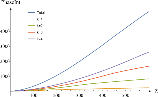
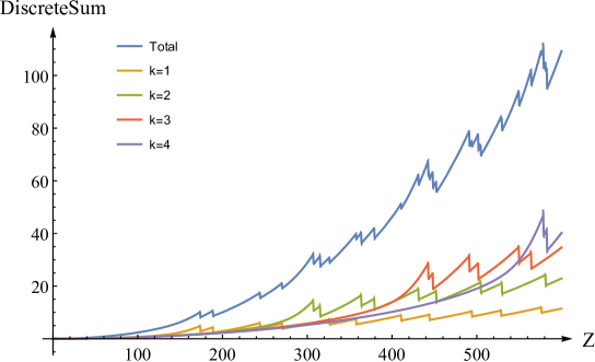
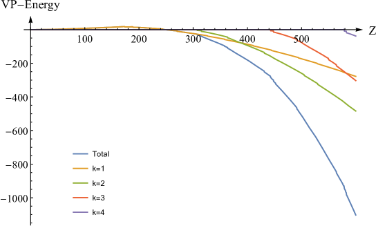
Figure 2: (Color online) $I(k)\,,\Sigma(k)\,,\hbox{$\cal E$}_{VP,k}^{ren}(Z)$ and $I_{tot}=\sum_{k=1}^{4}I(k)\,,S_{tot}=\sum_{k=1}^{4}S(k)\,,\hbox{$\cal E$}_{VP,tot}^{ren}(Z)=\sum_{k=1}^{4}\hbox{$\cal E$}_{VP,k}^{ren}(Z)$ on the interval $0<Z<600$ .

The partial VP-energies $\hbox{$\cal E$}_{VP,k}^{ren}(Z)$ are shown in Fig.2(c). Note that the behavior of $k=1$ channel is different from the others, since in this channel the structure of the renormalization coefficient $\zeta_{1}$ differs from those with $k>1$ by the perturbative (Uehling) contribution to VP-energy $\hbox{$\cal E$}^{(1)}_{VP}(Z)$. It is indeed the latter term in the total VP-energy, which is responsible for an almost quadratic growth with $Z$ of VP-energy on the interval $0<Z<Z_{cr,1}$. The global change in the behavior of $\hbox{$\cal E$}_{VP,1}^{ren}(Z)$ from the perturbative quadratic growth for $Z\ll Z_{cr,1}$, when the dominant contribution comes from $\hbox{$\cal E$}^{(1)}_{VP}(Z)$, to the regime of decrease into the negative range with increasing $Z$ beyond $Z_{cr,1}$ is shown below in Figs.3,4.

Figure 3: $\hbox{$\cal E$}_{VP,+}^{ren}(Z)\,,\ \hbox{$\cal E$}_{VP,-}^{ren}(Z)\,,\ \hbox{$\cal E$}_{VP}^{ren}(Z)$ on the interval $10\leqslant Z\leqslant 240$ (sphere).

Figure 4: $\hbox{$\cal E$}_{VP,+}^{ren}(Z)\,,\ \hbox{$\cal E$}_{VP,-}^{ren}(Z)\,$ on the interval $10\leqslant Z\leqslant 240$ (ball).

At the same time, in the channels with $k>1$ the quadratic perturbative contribution is absent. Therefore upon renormalization (28-30), which removes the quadratic component in $I(k)$ and $\Sigma(k)$, just after first level diving $\hbox{$\cal E$}_{VP,k}^{ren}(Z)$ reveal with increasing $Z$ a well-pronounced decrease into the negative range.

The final answers for the total VP-energy achieved this way are

$$\hbox{$\cal E$}_{VP}^{ren}(300)=-23.3\ ,\quad\hbox{$\cal E$}_{VP}^{ren}(600)=-1102.7\ .$$ (42)

On this interval of $Z$ the decrease of the total VP-energy into the negative range proceeds very fast, but with further growth of $Z$ the decay rate becomes smaller. In particular,

$$\hbox{$\cal E$}_{VP}^{ren}(1000)=-8398.6\ .$$ (43)

while the reasonable estimate of asymptotical behavior of $\hbox{$\cal E$}_{VP}^{ren}(Z)$ as a function of $Z$, achieved from the interval $1000<Z<3000$, reads

$$\hbox{$\cal E$}_{VP}^{ren}(Z)\sim-Z^{4}/R(Z)\ .$$ (44)

V Spontaneous positron emission

Now — having dealt with the general properties of VP-effects this way — let us consider more thoroughly the interval $10\leqslant Z\leqslant 240$, when only two first levels $1s_{1/2}\,,\ 2p_{1/2}$ with opposite parity $(\pm)$ have already dived into the lower continuum at $Z_{cr,1}$ and $Z_{cr,2}$. The behavior of the fixed parity $\hbox{$\cal E$}_{VP,\pm}^{ren}(Z)$ for the charged sphere and ball source configurations is shown in Figs.3,4. Note that the only difference between sphere and ball is the small shift of $Z_{cr,i}$ and the general magnitude of VP-energy, which in the ball case is $\simeq(6/5)\times$VP-energy for the sphere, that is quite close to the ratio of their classical electrostatic self-energies $3Z^{2}\alpha/5R$ and $Z^{2}\alpha/2R$.

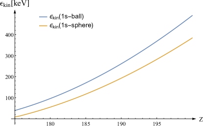
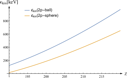
Figure 5: (Color online)  $\epsilon_{kin}(Z)$ with definite parity on the pertinent intervals of $Z$ for sphere and ball source configurations and (a): 1s-channel (even); (b): 2p-channel (odd).

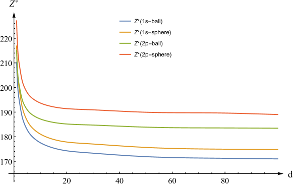
Figure 6: (Color online)  $Z^{\ast}(d)$ for $1\leqslant d\leqslant 100$.

General theory Greiner et al. (1985); Plunien et al. (1986); Greiner and Reinhardt (2009); Rafelski et al. (2017), based on the framework Fano (1961), predicts that after diving such a level transforms into a metastable state with lifetime $\sim 10^{-19}$ sec, afterwards there occurs the spontaneous positron emission accompanied with vacuum shells formation according to Fano rule (23). An important point here is that due to spherical symmetry of the source during this process all the angular quantum numbers and parity of the dived level are preserved by metastable state and further by positrons created. Furthermore, the spontaneous emission of positrons should be caused solely by VP-effects without any other channels of energy transfer.

So for each parity the energy balance suggests the following picture of this process. The rest mass of positrons is created just after level diving via negative jumps in the VP-energy at corresponding $Z_{cr,i}$, which are exactly equal to $2\times mc^{2}$ in accordance with two possible spin projections. However, to create a real positron scattering state, which provides a sufficiently large probability of being in the immediate vicinity of the Coulomb source, it is not enough due to electrostatic reflection between positron and Coulomb source. This circumstance has been outlined first in Refs.  Reinhardt et al. (1981); *Mueller1988; Ackad and Horbatsch (2008), and explored quite recently with more details in Refs. Popov et al. (2018); *Novak2018; *Maltsev2018; Maltsev et al. (2019); *Maltsev2020. From the analysis presented above there follows that to supply the emerging vacuum positrons with corresponding reflection energy, an additional decrease of $\hbox{$\cal E$}_{VP}^{ren}(Z)$ in each parity channel is required. So we are led to the following energy balance conditions for spontaneous positrons emission after level diving at $Z_{cr,i}$

$$\hbox{$\cal E$}_{VP,\pm}^{ren}(Z_{cr,i}+0)-\hbox{$\cal E$}_{VP,\pm}^{ren}(Z)=2\,\epsilon_{kin}(Z)\ ,$$ (45)

where $\epsilon_{kin}(Z)$ is the positron kinetic energy and it is assumed that for each parity positrons are created in pairs with opposite spin projections. In agreement with Refs. Popov et al. (2018); *Novak2018; *Maltsev2018; Maltsev et al. (2019); *Maltsev2020, in the considered range of $Z$ the spontaneous positrons are limited to the energy $0<\epsilon_{kin}(Z)<800$ (see Fig.5), while the related natural resonance widths do not exceed a few KeV Marsman and Horbatsch (2011); *Maltsev2020a.

It is also useful to introduce the parameter $d$ by means of relation

$$\epsilon_{kin}(Z)=Z\alpha/d\ ,$$ (46)

which can be interpreted as the distance from the center of the Coulomb source and the conditional point of the vacuum positron creation. Upon solving eqs. (45,46) with respect to $Z$, one finds that the vacuum positron emission is quite sensitive to $d$, as it is clearly seen in Fig.6. The reasonable choice for $d$ is approximately one electron Compton length $\lambda_{C}$ ($=1$ in the units accepted). The latter is a rough estimate for the average radius of vacuum shells, created simultaneously with the positron emission. Therefore it provides the most favorable conditions for positron production, from the point of view of both the charge distribution and the creation of a specific lepton pair.

However, the calculations performed show unambiguously that for such $d$ the emission of vacuum positrons cannot occur earlier than $Z$ exceeds $Z^{\ast}(1s)=217\,,Z^{\ast}(2p)=227$ (sphere), $Z^{\ast}(1s)=211\,,Z^{\ast}(2p)=215$ (ball) (to compare with $Z_{cr,1}=173.6\,,Z_{cr,2}=188.5$ (sphere), $Z_{cr,1}=170\,,Z_{cr,2}=183.1$ (ball)). Note also that $Z^{\ast}$ increase very rapidly for $d<\lambda_{C}$. In particular, already for $d=2/3$ one obtains $Z^{\ast}(1s)=233\,,Z^{\ast}(2p)=244$ (sphere), $Z^{\ast}(1s)=224\,,Z^{\ast}(2p)=229$ (ball). Such $Z^{\ast}$ lie far beyond the interval $170\leqslant Z\leqslant 192$, which is nowadays the main region of theoretical and experimental activity in heavy ions collisions aimed at the study of such VP-effects  Popov et al. (2018); Maltsev et al. (2019); Gumberidze et al. (2009); Ter-Akopian et al. (2015); Ma et al. (2017). In the ball source configuration the condition $170\leqslant Z^{\ast}\leqslant 192$ is fulfilled by $1s$-channel for $d>3\lambda_{C}$ and $d>5\lambda_{C}$ by $2p$-channel, but although such result can considered as the encouraging one, it should be noted that it is achieved within the model (2,3) with a strongly underestimated size of the Coulomb source in comparison with the real two heavy-ion super-critical configuration.

It would be worth to note that if allowed by the lepton number, spontaneous positrons can by no means be emitted also just beyond the corresponding diving point. In particular, for $d=137$ (one Bohr radius) one obtains $Z^{\ast}(1s)\simeq 174.0\,,Z^{\ast}(2p)\simeq 188.8$ (sphere), $Z^{\ast}(1s)\simeq 170.7\,,Z^{\ast}(2p)\simeq 183.3$ (ball), what is already quite close to corresponding $Z_{cr,i}$. But in this case they appear in states localized far enough from the Coulomb source with small $\epsilon_{kin}\sim 0.01$ and so cannot be distinguished from those emerging due to nuclear conversion. To the contrary, vacuum positrons created with $d\simeq\lambda_{C}$ possess a number of specific properties Popov et al. (2018); *Novak2018; *Maltsev2018; Maltsev et al. (2019); *Maltsev2020; Greiner et al. (1985), which allow for an unambiguous detection, but the charge of the Coulomb source should be taken in this case not less than $Z^{\ast}\simeq 210$. The negative result of early investigations at GSI Müller-Nehler and Soff (1994) can be at least partially explained by the last circumstance. Moreover, estimating the self-energy contribution to the radiative part of QED effects due to virtual photon exchange near the lower continuum shows Roenko and Sveshnikov (2018) that it is just a perturbative correction to essentially nonlinear VP-effects caused by fermionic loop and so yields only a small increase of $Z_{cr,i}$ and of other VP-quantities under question.

VI Concluding remarks

Thus, lepton number poses serious questions for both theory and experiment dealing with Coulomb super-criticality. Any reliable answer concerning the spontaneous positron emission — either positive or negative — is important for our understanding of the nature of this number. For the quantities like charge and spin, which should be also shared by vacuum shells if the spontaneous emission takes place, there are much less questions due to extended models of baryons as topological quantum solitons, including skyrmeons Adkins et al. (1983); *Holzwarth_1986, chiral quark-pion models Weigel (2007) and/or chiral bags Hosaka and Toki (2001). Apart from charge and spin, which can be defined as extended quantities for a quantum soliton in a general framework Rajaraman (1982); Dubikovsky and Sveshnikov (1994), these models define also the baryon number by means of the non-trivial topology of underlying $\sigma$-fields as a conserved quantity with extended spatial distribution. But the lepton number is different, since so far leptons show up as point-like particles with no indications on existence of any kind intrinsic structure.

Recent papers Popov et al. (2018); *Novak2018; *Maltsev2018; Maltsev et al. (2019); *Maltsev2020, aimed at the detailed study of spontaneous positron emission in slow heavy-ion collisions, have shown that one could expect a clear signal of transition to the super-critical mode for bare nuclei with the highest $Z=96$, whose colliding trajectories are close to head-on ones. These results look quite promising, but one should keep in mind that the slow head-on collisions of charged particles are highly unstable with respect to deviations in the transverse plane. Meanwhile, the case under consideration implies the scenario of colliding beams with total number of particles not less than $10^{6}$, hence the deviations of colliding trajectories due to interparticle interactions in the beam are inevitable. The large mass of nuclei does not matter, since it is compensated by the almost equally large charge. So one should expect that the most part of such slow collisions reduces to the peripheral ones, which cannot be reliably distinguished from the nuclear conversion. To reduce such instability one should consider more complicated collisions, which are based on the regular polyhedron symmetry Weyl (2015) — synchronized slow heavy-ion beams move from the vertices of the polyhedron towards its center. The simplest collision of such kind contains 4 beams, arranged as the mean lines of the tetrahedron with the intersection angle $\vartheta=2\arcsin(\sqrt{2/3})\simeq 109^{\small 0}\,28^{\prime}$, akin to s-p hybridized tetrahedron carbon bonds. The next and probably the most preferable one is the 6-beam configuration, reproducing 6 semi-axes of the rectangular coordinate frame . The advantage of such many-beam collisions is also that it requires significantly lower ion charges to attain the super-critical region. On the other hand, such collisions require serious additional efforts for their implementation. Therefore, an additional tasty candy is needed to arouse sufficient interest in such a project, and it is really possible, but this issue will be discussed in a separate paper.

VII Acknowledgments

The authors are very indebted to Dr. O.V.Pavlovsky and P.A.Grashin from MSU Department of Physics and to A.S.Davydov from Kurchatov Center for interest and helpful discussions. This work has been supported in part by the RF Ministry of Sc. $\&$ Ed. Scientific Research Program, projects No. 01-2014-63889, A16-116021760047-5, and by RFBR grant No. 14-02-01261. The research is carried out using the equipment of the shared research facilities of HPC computing resources at Lomonosov Moscow State University.

References

- Rafelski et al. (2017) J. Rafelski, J. Kirsch, B. Müller, J. Reinhardt, and W. Greiner, “Probing QED Vacuum with Heavy Ions,” in New Horizons in Fundamental Physics, FIAS Interdisciplinary Science Series (Springer, 2017) pp. 211–251.
- Kuleshov et al. (2015a) V. M. Kuleshov, V. D. Mur, N. B. Narozhny, A. M. Fedotov, and Y. E. Lozovik, Jetp Lett. 101, 264 (2015a).
- Kuleshov et al. (2015b) V. M. Kuleshov, V. D. Mur, N. B. Narozhny, A. M. Fedotov, Y. E. Lozovik, and V. S. Popov, Physics-Uspekhi 58, 785 (2015b).
- Godunov et al. (2017) S. I. Godunov, B. Machet, and M. I. Vysotsky, Eur. Phys. J. C 77, 77:782 (2017).
- Davydov et al. (2017) A. Davydov, K. Sveshnikov, and Y. Voronina, Int. J. Mod. Phys. A 32, 1750054 (2017).
- Voronina et al. (2017a) Y. Voronina, A. Davydov, and K. Sveshnikov, Theor. Math. Phys. 193, 1647 (2017a).
- Voronina et al. (2017b) Y. Voronina, A. Davydov, and K. Sveshnikov, Phys. Part. Nucl. Lett. 14, 698 (2017b).
- Popov et al. (2018) R. Popov, A. Bondarev, Y. Kozhedub, I. Maltsev, V. Shabaev, I. Tupitsyn, X. Ma, G. Plunien, and T. Stöhlker, Eur. Phys. J. D 72, 115 (2018).
- Novak et al. (2018) O. Novak, R. Kholodov, A. Surzhykov, A. N. Artemyev, and T. Stöhlker, Phys. Rev. A 97, 032518 (2018).
- Maltsev et al. (2018) I. A. Maltsev, V. M. Shabaev, R. V. Popov, Y. S. Kozhedub, G. Plunien, X. Ma, and T. Stöhlker, Phys. Rev. A 98, 062709 (2018).
- Roenko and Sveshnikov (2018) A. Roenko and K. Sveshnikov, Phys. Rev. A 97, 012113 (2018).
- Maltsev et al. (2019) I. A. Maltsev, V. M. Shabaev, R. V. Popov, Y. S. Kozhedub, G. Plunien, X. Ma, T. Stöhlker, and D. A. Tumakov, Phys. Rev. Lett. 123, 113401 (2019).
- Popov et al. (2020) R. V. Popov, V. M. Shabaev, D. A. Telnov, I. I. Tupitsyn, I. A. Maltsev, Y. S. Kozhedub, A. I. Bondarev, N. V. Kozin, X. Ma, G. Plunien, T. Stöhlker, D. A. Tumakov, and V. A. Zaytsev, Phys. Rev. D 102, 076005 (2020).
- Greiner et al. (1985) W. Greiner, B. Müller, and J. Rafelski, Quantum Electrodynamics of Strong Fields, 2nd ed. (Springer, Berlin, 1985).
- Plunien et al. (1986) G. Plunien, B. Müller, and W. Greiner, Phys. Rep. 134, 87 (1986).
- Greiner and Reinhardt (2009) W. Greiner and J. Reinhardt, Quantum Electrodynamics, 4th ed. (Springer-Verlag Berlin Heidelberg, 2009).
- Ruffini et al. (2010) R. Ruffini, G. Vereshchagin, and S.-S. Xue, Phys. Rep. 487, 1 (2010).
- Reinhardt et al. (1981) J. Reinhardt, B. Müller, and W. Greiner, Phys. Rev. A 24, 103 (1981).
- Müller et al. (1988) U. Müller, T. de Reus, J. Reinhardt, B. Müller, W. Greiner, and G. Soff, Phys. Rev. A 37, 1449 (1988).
- Ackad and Horbatsch (2008) E. Ackad and M. Horbatsch, Phys. Rev. A 78, 062711 (2008).
- Tupitsyn et al. (2010) I. I. Tupitsyn, Y. S. Kozhedub, V. M. Shabaev, G. B. Deyneka, S. Hagmann, C. Kozhuharov, G. Plunien, and T. Stohlker, Phys. Rev. A 82, 042701 (2010).
- Wichmann and Kroll (1956) E. H. Wichmann and N. M. Kroll, Phys. Rev. 101, 843 (1956).
- Gyulassy (1975) M. Gyulassy, Nucl. Phys. A 244, 497 (1975).
- Brown et al. (1975a) L. Brown, R. Cahn, and L. McLerran, Phys. Rev. D 12, 581 (1975a).
- Brown et al. (1975b) L. Brown, R. Cahn, and L. McLerran, Phys. Rev. D 12, 596 (1975b).
- Brown et al. (1975c) L. Brown, R. Cahn, and L. McLerran, Phys. Rev. D 12, 609 (1975c).
- Mohr et al. (1998) P. J. Mohr, G. Plunien, and G. Soff, Phys. Rep. 293, 227 (1998).
- Davydov et al. (2018a) A. Davydov, K. Sveshnikov, and Y. Voronina, Int. J. Mod. Phys. A 33, 1850004 (2018a).
- Davydov et al. (2018b) A. Davydov, K. Sveshnikov, and Y. Voronina, Int. J. Mod. Phys. A 33, 1850005 (2018b).
- Sveshnikov et al. (2019a) K. Sveshnikov, Y. Voronina, A. Davydov, and P. Grashin, Theor. Math. Phys. 198, 331 (2019a).
- Sveshnikov et al. (2019b) K. Sveshnikov, Y. Voronina, A. Davydov, and P. Grashin, Theor. Math. Phys. 199, 533 (2019b).
- Sveshnikov and Voronina (2022) K. Sveshnikov and Y. Voronina, In preparation (2022).
- Itzykson and Zuber (1980) C. Itzykson and J.-B. Zuber, Quantum Field Theory (McGraw-Hill, 1980).
- Fano (1961) U. Fano, Phys. Rev. 124, 1866 (1961).
- Voronina et al. (2019) Y. Voronina, K. Sveshnikov, P. Grashin, and A. Davydov, Physica E 106, 298 (2019).
- Rajaraman (1982) R. Rajaraman, Solitons and Instantons, 1st ed. (North-Holland Publishing Company, 1982).
- Sveshnikov (1991) K. Sveshnikov, Phys. Lett. B 255, 255 (1991).
- Sundberg and Jaffe (2004) P. Sundberg and R. L. Jaffe, Ann. Phys. 309, 442 (2004).
- Zeldovich and Popov (1972) Y. B. Zeldovich and V. S. Popov, Soviet Physics Uspekhi 14, 673 (1972).
- Marsman and Horbatsch (2011) A. Marsman and M. Horbatsch, Phys. Rev. A 84, 032517 (2011).
- Maltsev et al. (2020) I. Maltsev, V. Shabaev, V. Zaytsev, and et al., Opt. Spectrosc. 128, 1100 (2020).
- Gumberidze et al. (2009) A. Gumberidze, T. Stöhlker, H. F. Beyer, F. Bosch, A. Bräuning-Demian, S. Hagmann, C. Kozhuharov, T. Kühl, R. Mann, P. Indelicato, W. Quint, R. Schuch, and A. Warczak, Nucl. Instr. & Meth. in Phys. Research B 267, 248 (2009).
- Ter-Akopian et al. (2015) G. M. Ter-Akopian, W. Greiner, I. Meshkov, Y. Oganessian, J. Reinhardt, and G. Trubnikov, Int. J. Mod. Phys. E 24, 1550016 (2015).
- Ma et al. (2017) X. Ma, W. Wen, S. Zhang, D. Yu, R. Cheng, J. Yang, Z. Huang, H. Wang, X. Zhu, X. Cai, Y. Zhao, L. Mao, J. Yang, X. Zhou, H. Xu, Y. Yuan, J. Xia, H. Zhao, G. Xiao, and W. Zhan, Nucl. Instr. & Meth. in Phys. Research B 408, 169 (2017).
- Müller-Nehler and Soff (1994) U. Müller-Nehler and G. Soff, Phys.Rep. 246, 101 (1994).
- Adkins et al. (1983) G. S. Adkins, C. R. Nappi, and E. Witten, Nucl. Phys. B 228, 552 (1983).
- Holzwarth and Schwesinger (1986) G. Holzwarth and B. Schwesinger, Reports on Progress in Physics 49, 825 (1986).
- Weigel (2007) H. Weigel, Chiral Soliton Models for Baryons, Vol. 743 of Lecture Notes in Physics (Springer, 2007).
- Hosaka and Toki (2001) A. Hosaka and H. Toki, Quarks, Baryons and Chiral Symmetry (World Scientific, 2001).
- Dubikovsky and Sveshnikov (1994) A. Dubikovsky and K. Sveshnikov, Phys. Lett. B 321, 80 (1994).
- Weyl (2015) H. Weyl, Symmetry, Vol. 104 of Princeton Science Library (Princeton University Press, 2015).